the Creative Commons Attribution 4.0 License.
the Creative Commons Attribution 4.0 License.
 | 13 Sep 2022
Ice crystal images from optical array probes: classification with convolutional neural networks
Louis Jaffeux
Alfons Schwarzenböck
Pierre Coutris
Christophe Duroure
Although airborne optical array probes (OAPs) have existed for decades, our ability to maximize extraction of meaningful morphological information from the images produced by these probes has been limited by the lack of automatic, unbiased, and reliable classification tools. The present study describes a methodology for automatic ice crystal recognition using innovative machine learning. Convolutional neural networks (CNNs) have recently been perfected for computer vision and have been chosen as the method to achieve the best results together with the use of finely tuned dropout layers. For the purposes of this study, The CNN has been adapted for the Precipitation Imaging Probe (PIP) and the 2DS Stereo Probe (2DS), two commonly used probes that differ in pixel resolution and measurable maximum size range for hydrometeors. Six morphological crystal classes have been defined for the PIP and eight crystal classes and an artifact class for the 2DS. The PIP and 2DS classifications have five common classes. In total more than 8000 images from both instruments have been manually labeled, thus allowing for the initial training. For each probe the classification design tries to account for the three primary ice crystal growth processes: vapor deposition, riming, and aggregation. We included classes such as fragile aggregates and rimed aggregates with high intra-class shape variability that are commonly found in convective clouds. The trained network is finally tested through human random inspections of actual data to show its real performance in comparison to what humans can achieve.
- Article
(4587 KB) - Full-text XML
- BibTeX
- EndNote


Accurately representing ice clouds in radiative transfer models is extremely challenging due to the high diversity of the crystal habits present in these clouds (Yi et al., 2016). Thus, improving the general understanding of ice–cloud feedback in the climate system requires a better understanding of the processes occurring in these clouds (Wyser, 1999). In addition, the impact of atmospheric conditions on microphysical processes and resulting crystal morphologies cannot be studied without having reliable measurements of crystal habits inside ice clouds.
The qualitative observation of ice crystals in clouds in the 20th century has led to numerous attempts toward their classification into multiple crystal habit categories. For example, Nakaya (1954), Magono and Lee (1966), and more recently Kikuchi et al. (2013) have produced general classifications for natural ice and snow crystals, the latter including 130 sub-classes, reflecting the high diversity in shapes one can expect from ice crystals. Related to the classification methodology, scientists have identified three primary pathways of ice crystal growth, namely vapor deposition, riming, and aggregation (Pruppacher and Klett, 2010). The respective role of each of the three processes in the formation of different types of ice crystals has been frequently addressed, for example for vapor deposition (Bailey and Hallett, 2009), graupel (Sukovich et al., 2009), and aggregation (Hobbs et al., 1974). However, since accurate and reliable in situ measurements of natural ice crystal morphology has been very challenging in ice clouds, the processes associated with the formation and evolution of atmospheric ice are still poorly understood (Baumgardner et al., 2012).
Optical array probes (OAPs) are high-frequency airborne imagers commonly used for in situ observation of ice crystals in clouds. They produce large numbers of ice crystal images with counting statistics that allow establishing particle size distributions within seconds.
Since OAPs were developed in the 1970s (Knollenberg, 1970), several attempts have been made to produce high-performance classification algorithms based on morphological descriptors. While mathematically simple, the feature extraction for pattern recognition of 2D hydrometeor images developed by Rahman et al. (1981) and Duroure (1982) gives insight on how morphological image analysis is useful to automatically categorize OAP images into different classes. Their approach works well with synthetic images of singular crystals that exhibit completely unambiguous orientations and idealized shapes (see Rahman et al., 1981). In practice, the overwhelming majority of observed ice crystals are not perfectly oriented, undergo multiple microphysical processes at different levels including aggregation, and show natural irregularities. Such methods are also limited by the pixel rendering of edges from the probes, which diminishes their performance. These limits were identified and reported in Korolev and Sussman (2000) wherein a feature-based classification technique was applied to 2DC data. More recently, this technique has been applied to images from the Cloud Particle Imager (CPI), an imager based on a charge-coupled device (CCD) with finer resolution and grayscale levels (Lawson et al., 2006; Lindqvist et al., 2012; Woods et al., 2018) based on criteria for 2D pattern recognition. Finally, Praz et al. (2018) used features from these previous studies and from Praz et al. (2017) in a new methodology called multinomial linear regression (MLR) to classify images from two different OAPs (2DS and HVPS) and the CPI. This classification tool has brought the feature-based approach to its highest maturity but is still very limited in its ability to quickly process and classify images. Furthermore, it was only roughly evaluated on two 1 min flight periods of the OLYMPEX campaign (Houze et al., 2017). In conclusion, the feature-based approach in its ultimate form is not only slow and trained specifically for a given context, but it also operates in a very distant manner to the way our brain identifies shapes and objects, potentially creating bias from feature definitions.
Considering the fact that computer vision has advanced in a way that today it can emulate the human brain's ability to recognize shapes and objects (Russakovsky et al., 2015), a different approach to the classification problem was favored in the present study. Instead of relying on designed features, a widespread and well-known method called convolutional neural network (CNN) (Krizhevsky et al., 2012; He et al., 2016) reproduces the human ability to identify complex shapes and objects and develops hierarchical sets of features from raw labeled data. During the time when the presented work was under development, CNN classification tools emerged for the CPI (Xiao et al., 2019; Przybylo et al., 2021); however, they still need to be adapted for OAP image data. In general, OAP images lack textural information (legacy data sets comprise black and white images, while newer probes have a maximum of four levels of gray) and also exhibit much coarser resolution ( photodiode array compared to a 1 megapixel camera), but they have the advantage of continuously imaging the sample volume between the probe arms, which is not the case when relying on a particle detector with comparably few CCD high-resolution grayscale images. As a result, the use of OAP instruments in airborne campaigns produces a more quantitative and statistically meaningful representation of the cloud microphysical state but with diminished morphological information (3D object projected to binary 2D image).
In Sect. 2 of this study, the OAP data and chosen morphological classes are presented. Then the CNN methodology for the automatic classification of ice crystals for the 2DS and the PIP probes is detailed in Sect. 3, together with the description of the training process and evaluations of the fully trained networks on the test set. Section 4 presents an evaluation of the performance of the two classification tools with random visual inspections. The conclusions are summarized in Sect. 5.
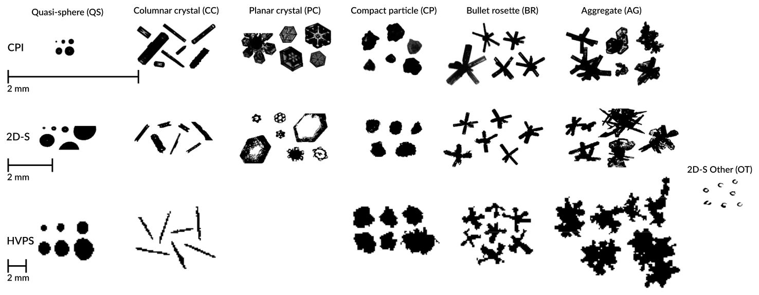
Figure 1Illustration of ice crystal habits from Praz et al. (2018) for different cloud-imaging probes.
The very first step of the convolutional neural network methodology is to build a database wherein images are associated with labels by an operator. This procedure implies that classes have to be defined beforehand. In the context of defining morphological classes, three items are mentioned and shortly discussed here.
-
The primary goal of our habit classification is to reveal ice crystal growth mechanisms inside a cloud. The designed classes in this study are rather comparable to those used in Praz et al. (2018) (shown in Fig. 1), which were themselves inspired by the pioneering work of Magono and Lee (1966). The chosen morphological classes primarily account for the three ice growth mechanisms of vapor deposition, aggregation, and riming. All possible crystal shapes are included in a rather limited number of classes without trying to implement the 130 classes (basically high-resolution grayscale CCD images) from Kikuchi et al. (2013).
-
The two probes' technical details are presented in Table 1. For the image analysis, only non-truncated images with maximum dimensions Dmax>300 µm (30 pixels, for 2DS) and Dmax>2 mm (20 pixels for PIP) have been classified. Below 300 µm, 2DS images are frequently distorted by diffraction effects (e.g., Vaillant de Guélis et al., 2019). This effect persists above this threshold to a lesser extent and led to the definition of a dedicated artifact class for the 2DS, labeled as diffracted particles (Dif). Heavily rimed aggregates are rather large and thus rarely observed in 2DS images, since they are most likely truncated and thus automatically discarded. Moreover, looking at the 2DS images, strikingly well-detailed combinations of columns, plates, and dendrites were found. Although sometimes it is not clear whether aggregation may have occurred during their formation, the absence of riming and the influence of diffusional growth are undeniable. The corresponding class for those images is denoted complex assemblages of plates, columns, or dendrites (complex assemblages, CAs). The coarse resolution of the PIP makes it practically impossible to discern details such as transparency and sharp edges associated with the diffusional growth. For this reason mixed combinations of columns, plates, and dendrites (CAs) cannot be clearly distinguished from what is designated as fragile aggregates (FAs). Due to the lower threshold of utilized PIP images of 2 mm, capped columns and water drops are scarce in our training database and thus were not considered morphological classes for PIP images in this study.
-
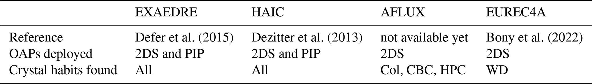
The data used were observed during several airborne research campaigns. Initially, HAIC (Dezitter et al., 2013) and EXAEDRE (Defer et al., 2015) were the main data sources for OAP images. Selecting data and labeling images manually, although being mandatory for a supervised classification scheme, is a long and strenuous process. Some classes were harder to find in these campaign data and motivated the use of two further campaigns (AFLUX and EUREC4A) to speed up filling these less populated habit classes (see Table 2).
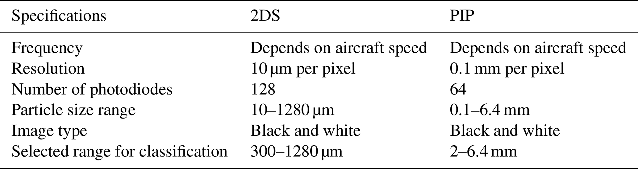
Table 2All the PIP images in the original data set originate from two events in the EXAEDRE campaign and three events of the HAIC campaign. The context of these events are thunderstorms in the Mediterranean Sea for EXAEDRE and mesoscale convective systems in French Guiana for HAIC. Most of the 2DS data also originate from the same events. The AFFLUX campaign data were extracted from a single flight in stratiform clouds in the Arctic to provide more Col, CBCs, and HPCs of various sizes. Finally, all the water droplets of the 2DS data set were captured during a single flight in liquid water clouds in the Caribbean Sea during the EUREC4A project.
Traditionally, the training set is comprised of randomly chosen images from the whole available database. Since all the classes are not represented equally in crystal numbers, an adjustment in the loss function should be made to account for the classes with lower representation. Still, an operator in charge of classifying these images would face the difficulty of classifying particles from images that stand between multiple classes or that are not identifiable because of ambiguous random projections. Defining a class dedicated to irregular crystals has been avoided, since we believe that, with the high variability associated with crystal shapes, it would be very dependent on the appreciation of the operators, who could eventually fit too many images into this “irregular” class. Moreover, the nature of the output of a CNN makes it possible to produce non-categorical results in order to express some level of ambiguity between two or more classes instead of simply stating its inability to identify the image.
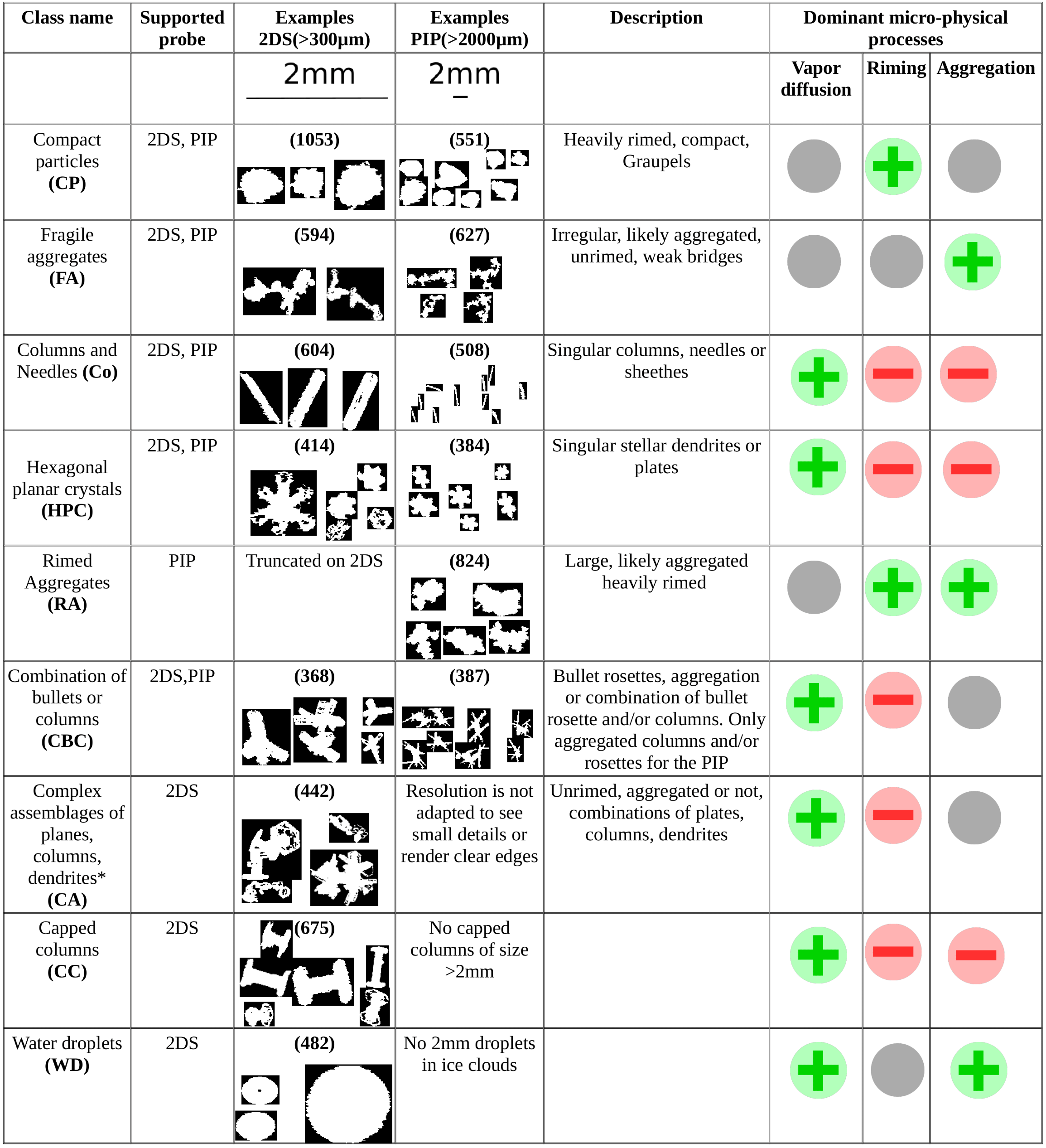
The overview of the nine microphysical habit classes accounted for in this study is presented in Table 3 and discussed below. Overall, nine morphological classes have been defined; five are common to the two probes: compact–graupel (CP), fragile aggregates (FAs), columns (Co), combination of columns and bullets (CBC), and hexagonal planar crystals (HPCs). Moreover, one class specific to the PIP consists of rimed aggregates (RAs), and three specific classes are added for the 2DS, namely water droplets (WDs), capped columns (CCs), and an artifact class (Dif) for out-of-focus images. Co, CCs, and HPCs are singular, unrimed crystal images that originated solely from diffusional growth. CBCs and CAs have mostly grown by deposition of water vapor and may result from aggregation of more than one particle but remain unrimed. FAs are products of aggregation of several unrimed or lightly rimed particles, while RAs show an evident fluffy aspect, characteristic of the collection and freezing of supercooled droplets on the crystal's surface. Finally, CPs are ice particles with the highest degree of riming, in which the contribution of the two other processes is invisible. In every case, growth by vapor diffusion cannot be ruled out as it continuously contributes to ice production in a cloud.
Some images obtained with OAPs are commonly found to be ambiguous in the sense that they do not clearly belong to exactly one class. One could justify the inability of non-ambiguous classification of every image with two independent explanations. First of all, OAPs are 2D binary low-resolution imagers. Random orientations combined with the lack of surface information and the low number of pixels occasionally hide important features that are required to identify certain crystal types. For example, a plate seen from the side could be strictly impossible to differentiate from a column. Secondly, the definition of crystal habit classes is lacunar by design, and it is unavoidable that some crystals might be found not to belong to any class or to belong to more than one class. As a matter of fact, the classes defined here or in general in the literature (Kikuchi et al., 2013 or Magono and Lee, 1966) are only landmarks for local clusters in a continuous multivariate space wherein ice crystals happen to be moved by the microphysical processes that are active in their respective environment during their lifetime. Taking into account these two factors, it was decided in the process of forming the initial labeled data set for each probe that only unambiguous images were selected for the test, validation, and training sets rather than randomly selected images from the available data and trying to classify all of them. Since the classification is meant to be applied to actual data, it is important that we provide a way to quantify its performance and the uncertainty associated with it (discussed in Sect. 4).
Table 3The nine microphysical classes used in the classifications. Green circles mean the microphysical process recently played a role in the particle's growth. Red circles mean the microphysical process certainly did not occur in the particle's growth. The gray circle means the microphysical process might have happened at some point, but there is no evidence of it happening recently. In parentheses is the number of images used in the original labeled database for each class. * Images shown for combinations of columns, plates, and dendrites are scaled down compared to other images so that they fit in the table properly.
This section presents the classification methodology that was applied to the two OAPs. First some insight is given on the implemented convolutional neural network (CNN) technique. Then the training methodology is detailed. Finally, the quality of the training is evaluated with independent test sets, and the results are discussed.
3.1 Convolutional neural network, general principles
CNN and similar deep learning techniques are largely used in medical image analysis (Tajbakhsh et al., 2016; Gao et al., 2019), but are also emerging in other research fields, for example in biology for plankton image analysis in Luo et al. (2018). Especially in medical image analysis, the success of CNN algorithms is evident. They are highly reliable and have, by design, the ability to learn hierarchically built complex features from raw data. CNN is therefore an incredibly pertinent technique for image analysis in general (Krizhevsky et al., 2012). The following architecture description presents the algorithm in its working state (for further information see Goodfellow et al., 2016), and its training for each of the two probes will be described in the next subsection.

Figure 2CNN architecture and building blocks. (a) Simplified architecture of convolutional neural networks. (b) Elementary operation at the heart of convolutions from http://intellabs.github.io/RiverTrail/tutorial/ (last access: 7 September 2022). (c) Illustration of maxPooling, found at https://medium.com/mlearning-ai/images-from-the-convolutional-world-596b4aa6cdae (last access: 7 September 2022).
When applied to computer vision, CNN algorithms consist of two parts: a feature extractor and a classifier (see Fig. 2a). Both of these have large sets of trainable parameters, which will be updated during the learning phase through gradient backward propagation. The feature extractor is hierarchically built with two initial building blocks: convolutional layers (Convlayers) and subsampling layers (maxPooling in our case) – both are illustrated in Fig. 2b and c, respectively. Convlayers can be seen as filters or masks. In practice, it is a square matrix with trainable values. The size of these filters is called their receptive field (here 3 by 3), and they are applied through a dot product to each pixel and all the pixels around in the receptive field. After normalization and use of an activation function, the convolution of the input by each filter produces a set of feature maps. They are then subsampled with a 2 by 2 maxPooling filter. Subsampling diminishes the noise induced by the previous convolution and summarizes the information contained for feature maps to its most crucial part. The output obtained from the subsampling layer is a set of square matrices with dimensions twice as small as the input. The number of filters of the next convolution step can therefore be doubled with no increase in computational cost, increasing the potential complexity of the algorithm and ultimately its ability to generalize and infer relevant abstracted features as we go into the deeper layers. Convlayers and maxPooling layers are repeated (see Fig. 2a) in the feature extracting part until every feature map is reduced to a 1 by 1 size.
Finally, a fully connected perceptron with one hidden layer serves as the classifier (right side in Fig. 2a) to attribute a class to the highly abstracted features extracted from the original input image. In this final stage, for individual images, probabilities are calculated to belong to any of the eligible classes. A minimum threshold (usually of 50 %) can eventually be applied to segregate images that failed to be identified by the algorithm. Actual model plots for both probes (PIP and 2DS) are provided in Fig. A2a and b, respectively.
Three state-of-the-art overfitting countermeasures were implemented in the initial architecture: namely, dropout layers were added between the subsampling and convolutional layers, an early stopping condition was set during the training phase, and batch normalization was applied.
The use of dropout allows training very complex models with a limited number of training data without overfitting (Srivastava et al., 2014). This method is applied only during training to the fully connected layer and to the convolutional layers (Park and Kwak, 2016, proved dropout usefulness on convolutions). An exponential number of shallow models sharing weights are improved during training. As a result, multiple confirmation paths emerge, each one of them focusing on essential features. The trained model becomes much more robust to noise and translations. The effect of dropout adds to the data augmentation layer, an early stopping condition, and the batch normalization to ensure that overfitting will not happen and that the ability of the model to generalize is enhanced as much as possible.
3.2 Training
An overview of the training methodology is given in Fig. 3. After labeling the data, the images are padded to the same size and randomly split into three subsets: test (20 %), validation (16 %), and training (64 %). The training set is used to teach the model. The feature extractor and the classifier presented in the previous subsection can be trained at the same time using the feed forward–backward error propagation scheme as represented in Fig. A1. After every epoch, which is completed when all the training data have been used to update the trainable parameters, the model is evaluated on the validation set to monitor its improvements and whether or not overfitting is occurring. Whenever the loss function computed on the validation set fails to improve five epochs in a row, the training is stopped. If the validation loss and accuracy are judged to be satisfactory, we proceed to evaluate the model with the test set. This last step produces the performance metrics shown in Fig. 4 (precision is the fraction of detections reported by the model that were correct, recall is the fraction of true events that were detected, and the f1 score is the harmonic mean of precision and recall (Goodfellow et al., 2016)).
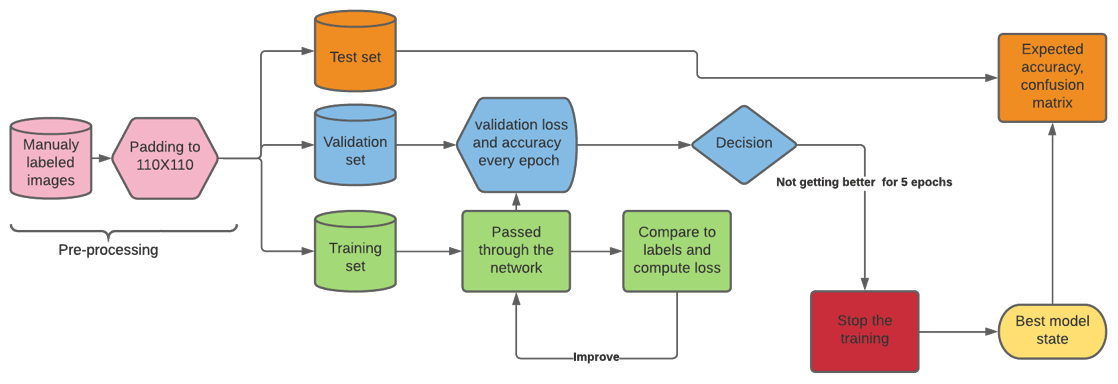
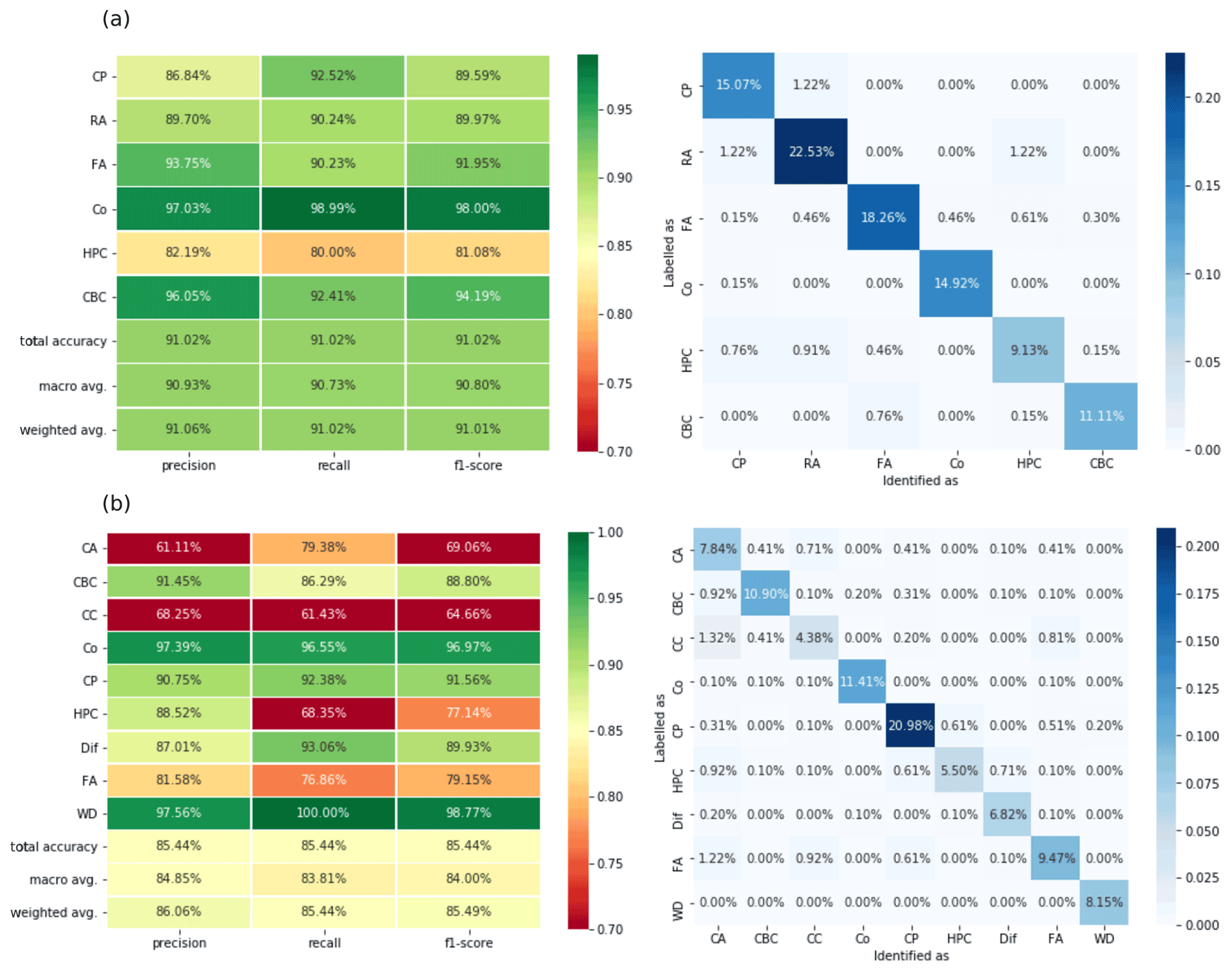
Figure 4Evaluation of training for each probe with an independent test set. (a) Left, classification report (PIP) obtained for the corresponding test set. Right, confusion matrix (PIP) obtained for the corresponding test set; values on the diagonal correspond to samples correctly classified. (b) Left, classification report (2DS) obtained for the corresponding test set. Right, confusion matrix (2DS) obtained for the corresponding test set. The matrix values are normalized so that they sum up to 100 %.
3.3 Training evaluation: results on test sets
Hyperparameter tuning was performed using the Keras built-in random search functionality (Chollet et al., 2015) and resulted in the values presented in Table A1. Other hyperparameters (dropout values and the number of neurons in the fully connected layer) also required tuning.
The PIP CNN model (Fig. A2a) was trained using stochastic gradient descent (SGD) with a batch size of 16 and a decay rate of 10 % every five epochs applied to the learning rate. Weights were initialized using the Glorot initialization with a uniform distribution (these are the default settings when using the Keras library; Chollet et al., 2015). The use of a RandomFlip layer (only active during training) as a first layer drastically improved the quality of the training. This layer randomly flips the input image horizontally (left–right flip), vertically (top–bottom flip), both ways, or not at all (with all four possibilities having the same probability) and thus produces more variety in orientations in the training data. An early stop condition was used in order to end the training, under the condition that the validation loss function did not improve in five epochs. In total, 1 634 438 parameters were trained to obtain this model. The performance of the model for the test set is described in Fig. 4a. Performance is high in general with an overall f1 score above 91.1 %. The worst recognizable class is HPCs with an f1 score of 81.08 %. The confusion matrix indicates some porosity between HPCs and RAs: eight RAs were identified as HPCs in the test set (1.22 % of the total). These results are hardly comparable with any results found in the literature, since PIP images are not usually used in classification algorithms.
The model corresponding to the 2DS (Fig. A2b) was trained using the same SGD approach as the PIP model, with a batch size of 16 and a decay rate of 10 % every five epochs applied to the learning rate. The same weight initialization method as the PIP model was performed and the same RandomFlip data augmentation layer was used during training. Finally, the same early stop condition terminated the training phase. The main difference between the two models was the input size increasing from 110 by 110 for PIP to 200 by 200 for the 2DS (Fig. A2b) and the depth of the first convolutional layer (64 filters for the 2DS against 32 for the PIP). As a result, an additional combination of the convolutional layer and subsampling layer (and dropout during training) had to be implemented and the size of the fully connected layer of the classifier had to be increased, taking into account that there are now 2048 1 by 1 cells in the final feature map array at the end of the feature extractor (512 for the PIP). 26 397 129 parameters were determined during the training. The observation of the classification report (left panel of Fig. 4b) indicates that some classes are very well identified, which are CBCs, Co, CPs, Dif, and WDs, while the remaining classes are less well recognized in the test set. Most of the confusion seems to result from images being misclassified in the CA class: 18.5 % of all CCs (1.32 % of the total), 11.4 % of all HPCs (0.92 % of the total), and 9.9 % of all FAs (1.22 % of the total) (see right panel of Fig. 4b). These results exhibit the difficulties we faced in defining a set of exhaustive classes with as few overlaps as possible. When looking at the image examples in Table 3, one can easily notice how CC, HPC, and CBC classes share similarities in their shapes with the CA class, which has much higher internal variability. The most comparable results we can relate to in the literature are those of Praz et al. (2018). They obtained an overall accuracy of 93.4 % for this probe but had two fewer classes, namely no comparable class to CC and one common class merging CA and FA. If we put together the CA and FA classes in the confusion matrix, considering that the images confused between the two classes are correctly identified (1.22 % and 0.41 % of the total), and ignore every image that was either identified or labeled as a capped column (9.15 % of the total), the total accuracy reaches 91.1 %, which mainly reflects how class definitions can affect the results, since the original databases had quite different origins.
First, the motivations for performing random inspections are given, then the methodology is discussed. Finally, the results are presented for both probes in the two last subsections.
4.1 Motivations and methodology for random inspections
Random inspections have two benefits. The primary benefit is to be able to compare the variability among human predictors and, particularly, between human predictors and the network. A secondary benefit is simply to produce more manually labeled data. In the case of misclassified images, the newly labeled data can be used to increase intra-class variability and the overall performance of the network.
In order to compare the implemented CNN algorithm with human performance, 10 scientists from the Laboratoire de Météorologie Physique were gathered and given the keys to recognizing the ice crystal classes during two meetings (one for each probe), wherein they were presented with all morphological classes and given a subset of images from each class from the training data as a reference point. At the end of each meeting they were tested on other images from the training data and assisted with the correction of their tests. This exercise was thought of as a way to improve their skills and as an opportunity to clear up some of the confusion that could remain; the results were nonetheless recorded.
Using data from the recent ICE-GENESIS campaign, 400 images were randomly extracted for the PIP and 500 for the 2DS. An html form was designed and shared with all the participants. They had to attribute a single class associated with a degree of confidence (not taken into account in the scoring) to each image, one after the other. Time spent on each image was recorded.
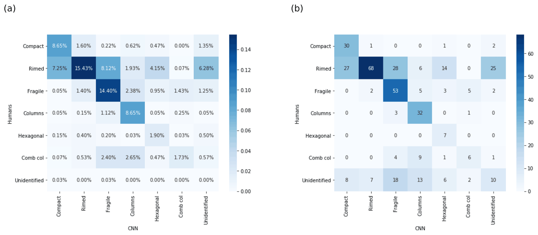
Figure 5Comparison between human and CNN results. (a) Confusion matrix (PIP); identification threshold at 50 % for the CNN results. (b) Mean confusion matrix (PIP) in numbers; identification threshold at 50 % for the CNN and human results. Overall, the agreement between them is 50.7 %. The expected porosity between CP and RA and between FA and RA seems to appear and is investigated in Fig. A3. Every one of the 40 images considered unidentified by the algorithm shows its highest score in the CP class.
4.2 Results
4.2.1 PIP
On average, each participant spent 1 h and 10 min completing the PIP form. Figure 5 details the overall results of the random inspections, and Fig. 5a displays all 4000 responses from the 10 operators, which are normalized, while Fig. 5b shows how the 400 images are classified by humans and the network in numbers. In this second case a majority rule is used to determine the class attributed by humans; if the majority (50 %) is not reached for a given image then the image is considered unidentified by humans. The inspected images belong mostly to the CP, RA, FA, and Col classes according to human inspection and CNN. Humans classified many more particles as RAs than the algorithm. Most of the images classified as RAs by humans and not by the CNN are either classified as CPs or FAs by the CNN. This confusion was expected since with randomly picked images, the chances were high to find ice crystals between those classes. When comparing the images for which the CNN and humans agree and disagree, respectively, for the three classes RA, FA, and CP (Fig. A3), it appears that the CNN has developed more consistent class definitions and is therefore superior to the humans in discriminating between the three classes. 25 images remain unidentified for the CNN and are classified as RAs by the humans (Fig. A4). Looking at their scores, the CNN is undecided about whether to classify them either in RA or CP, with neither of the two probabilities above 50 %. Therefore, one might want to merge RA and CP before applying the identification threshold in order to have the full estimate of the importance of riming. The porosity between RA and FA is somewhat less evident with the sampled images. Nevertheless, in order to have a better estimate of the importance of aggregation a similar approach could be applied.
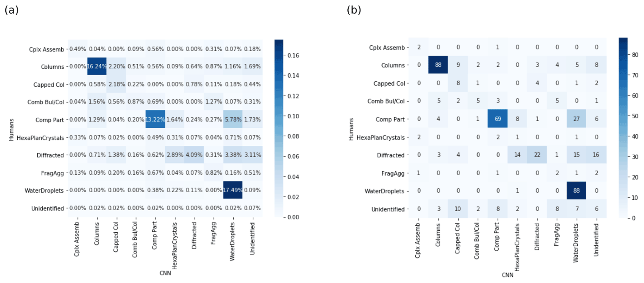
Figure 6Comparison between human and CNN results. (a) Confusion matrix (2DS); identification threshold at 50 % for the CNN results. (b) Mean confusion matrix (PIP) in numbers; identification threshold at 50 % for the CNN and human results. Overall, the agreement between them is 58.2 %. The expected porosity between CP and RA and between FA and RA seems to appear and is investigated in Fig. A3. Every one of the 40 images considered unidentified by the algorithm shows its highest score in the CP class.
4.2.2 2DS
On average, each participant spent 1 h and 18 min completing the confusion matrix (2DS), with the identification threshold at 50 % for the CNN results. DS forms (three forms were provided this time on demand by the participants) were also completed. Figure 6 details the overall results of the random inspections (same as Fig. 5 but for the 5000 responses and 500 images of the 2DS inspection data set). The inspected images belong mostly to WD, CP, Dif, and Col classes according to both humans and the CNN. With a limited number of classes present in the sample (only four out of nine), general agreement is found between the CNN and humans (58.2 %). The confusion matrices reveal that the Dif class is the most problematic class for the CNN. Indeed, the network spreads Dif between HPC and WD or does not manage to identify them. Additionally, despite being able to identify almost every WD as such, the algorithm puts some CPs in this class in addition to the aforementioned Dif. This can be explained by all three classes consisting of possibly small quasi-spherical or spherical particles. Humans and the CNN identified some CCs. When looking in more detail, it seems that both humans and the CNN were confused by small, sometimes diffracted sheaths and needles. Three out of 10 participants reported difficulties in classifying “H-shaped” images (shown in Fig. A5) that we would interpret as small diffracted columns (see Vaillant de Guélis et al., 2019). The CNN exhibits this issue as well and shows a lack of such particles in the original training database for the Dif class.
An automatic classification tool has been developed for two OAPs that are routinely used aboard research aircraft in the cloud observation community in general (Leroy et al., 2017; Defer et al., 2015; Houze et al., 2017; McFarquhar et al., 2011). Both probes, namely the 2DS and the PIP, produce 2D binary images at high frequency in different size ranges. Because of the inability to recognize ice crystal morphology from images with a limited number of pixels, the chosen ranges of 300–1280 µm for the 2D-S and 2000–6400 µm for the PIP do not overlap. Still, they provide us with complementary information and therefore the classification model for both probes is a strong asset for understanding cloud microphysical growth processes. The methodology presented in this paper was adapted from the most widespread image recognition technique, which attempts to reproduce the human brain's ability to learn and recognize shapes: the convolutional neural network. Two of these networks have been successfully trained for the two probes and were confronted with inspections by humans of unknown image data. The present study utilized image data from the HAIC and EXAEDRE projects in tropical and midlatitude convection (with pronounced crystal growth contributions from aggregation and riming), the AFLUX Arctic project to add vapor-diffusion-dominated growth images, and precipitating drops gathered within the EUREC4A project in the Caribbean Sea. By intention, we did not tune the methodology for a particular type of cloud, nor was it a goal to add contextual information (dynamic, thermodynamic, microphysical, or presumed morphological information on crystal populations) to the classification. The human inspection, rarely performed in the scope of applied artificial intelligence, provides a credible evaluation of the CNN tool's performance. The main conclusions of this study are the following.
-
Despite the low number of pixels of OAPs and their binary nature, it is possible for CNNs to learn features associated with the classes defined in Sect. 2.
-
The PIP CNN algorithm proved to be more reliable than humans for some classes that see a lot of porosity in field data (e.g., rimed aggregates, compact particles, and fragile aggregates).
-
Data assimilation has been made possible by running random inspections and should be used for both probes, especially for the 2DS, to increase the intra-class variabilities of the few represented habits.
-
Random inspections should be part of the classification routine (see Fig. A6), since this allows quantifying its performance, better understanding its results, and acquiring more labeled data, improving the representation of individual classes.
In summary, this study describes a new methodology for ice crystal morphological recognition from OAP images and a way of assessing its performance. Indeed, a systematic and consistent classification of OAP data can provide improved quantitative information on crystal habits by applying the presented methodology. In the near future, this should facilitate improved detailed microphysical studies, for example targeting habit-specific mass relationships (e.g., from Leinonen et al., 2021). Similar classification tools can easily be developed for other OAP probes, for example the cloud-imaging probe (CIP), the four-level grayscale CIP, and the high-volume precipitation spectrometer (HVPS). The CIP (pixel resolutions of 15 and 25 µm) mainly overlaps the 2DS size range, while the HVPS (up to 1.92 cm) would extend the maximum hydrometeor size for the morphological analysis compared to the PIP. Last but not least, common effort could be made in the global atmospheric sciences community in order to gather a common image database for each instrument, thereby agreeing on defined classes, so that we can develop and test universal future classification algorithms.
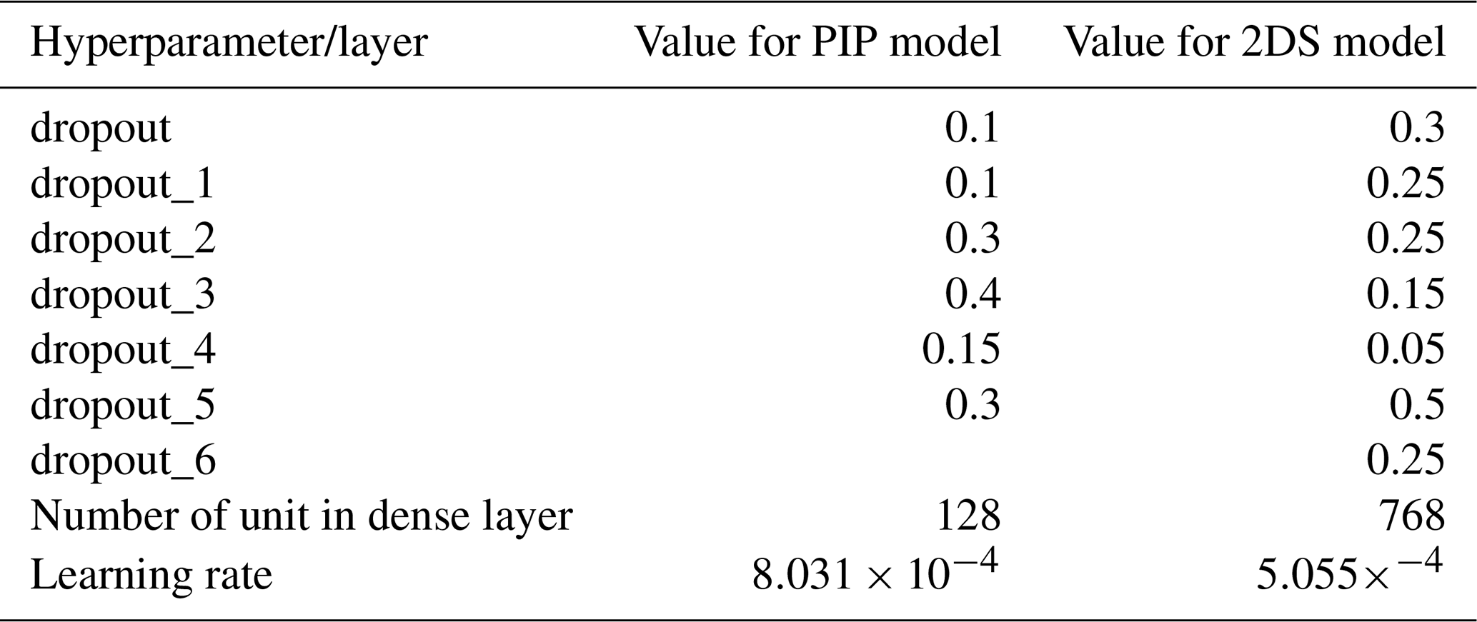

Figure A1The three steps leading to parameter improvement. (1) Forward pass: the image is passed through the network and an output is obtained. (2) An error is computed between this prediction and the target output. (3) This error is propagated by gradient descent back into the network to update the trainable parameters in the model.
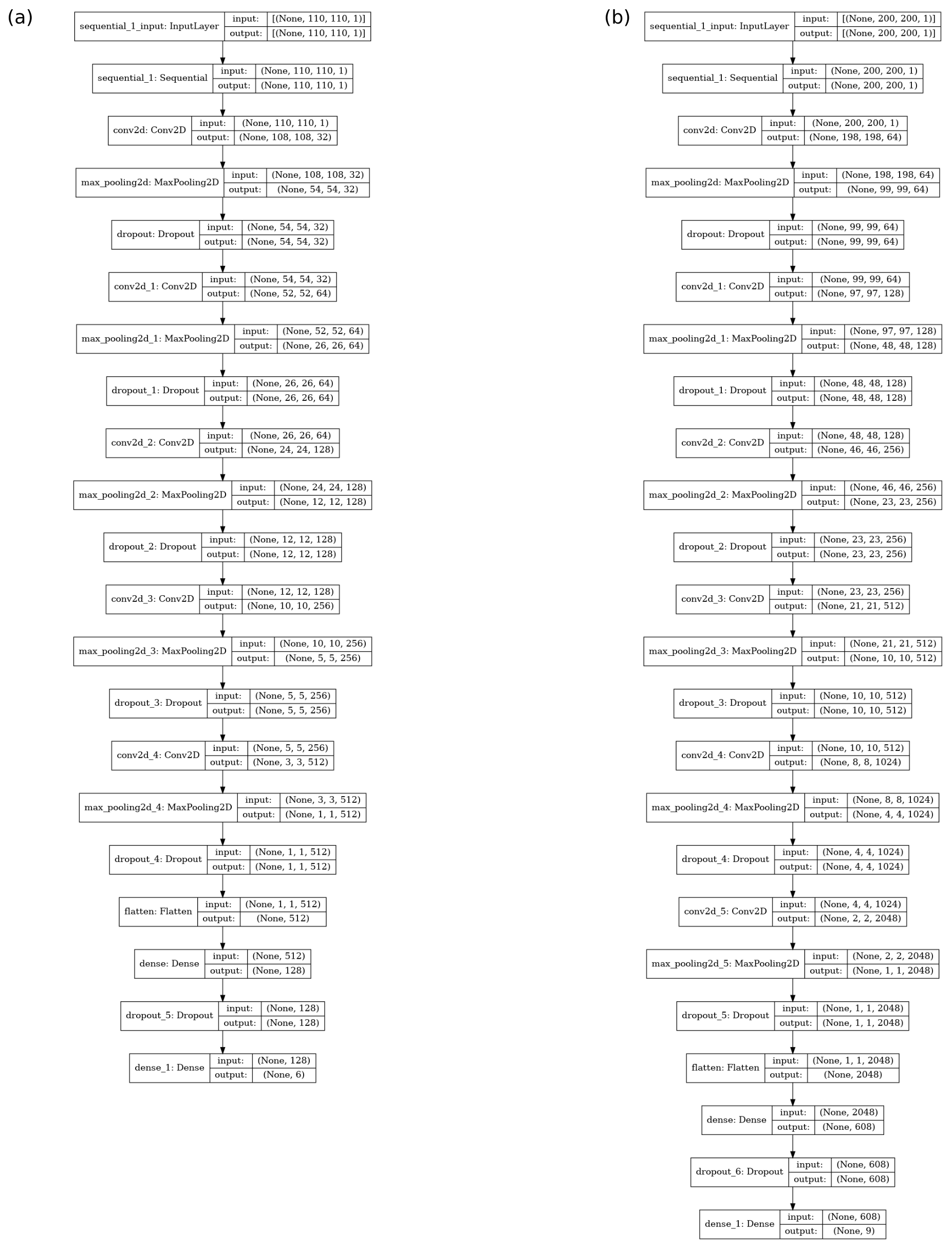
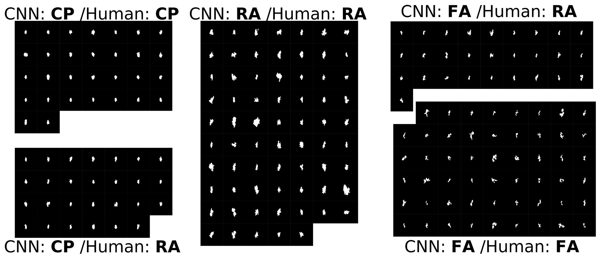
Figure A3Confusion between humans (majority rule) and the CNN for the RA, FA, and CP classes. The CNN predictions are more consistent than those of humans.
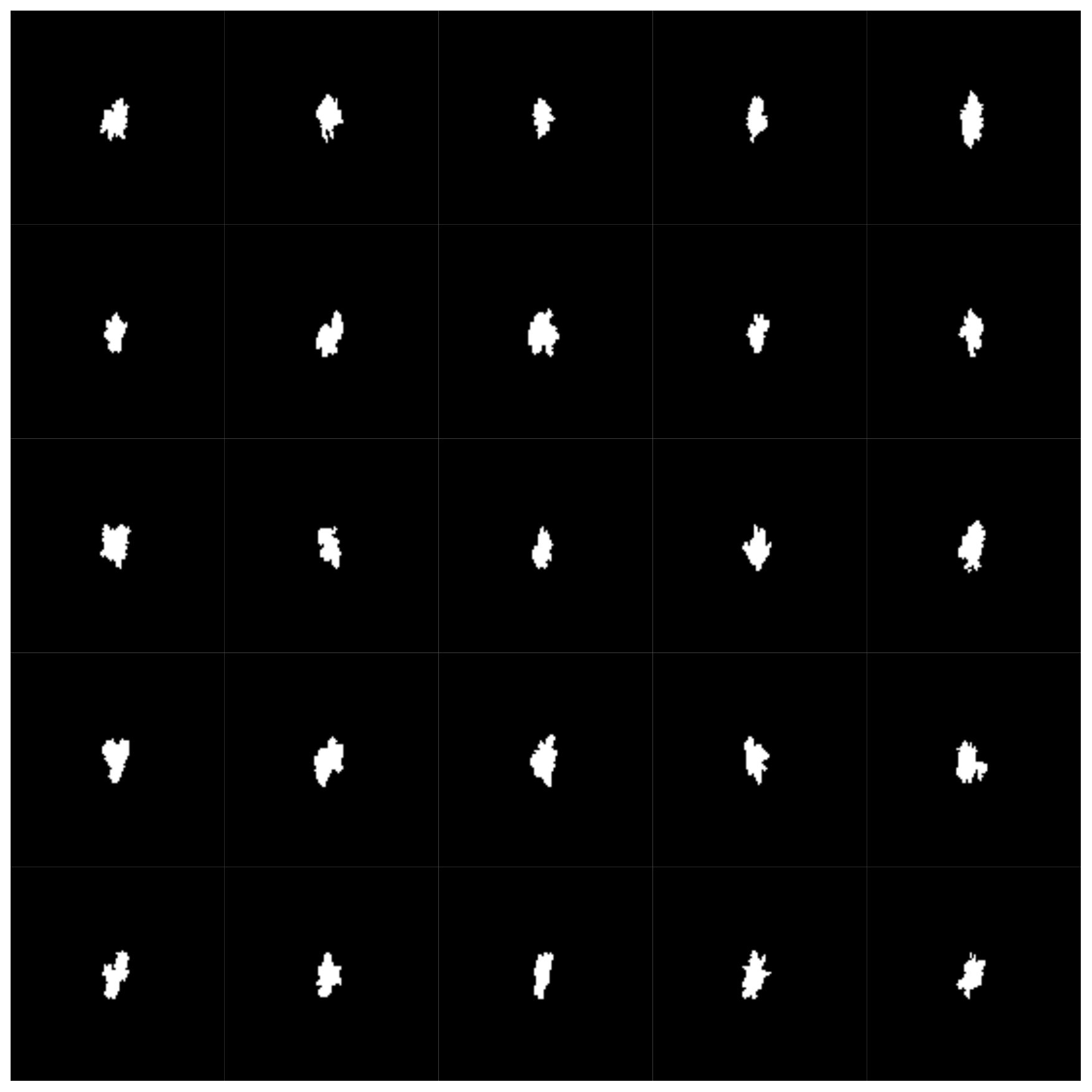
Figure A4Images identified as RAs by participants and unidentified by the algorithm. The algorithm gave all these images a high score in both RA and CP.
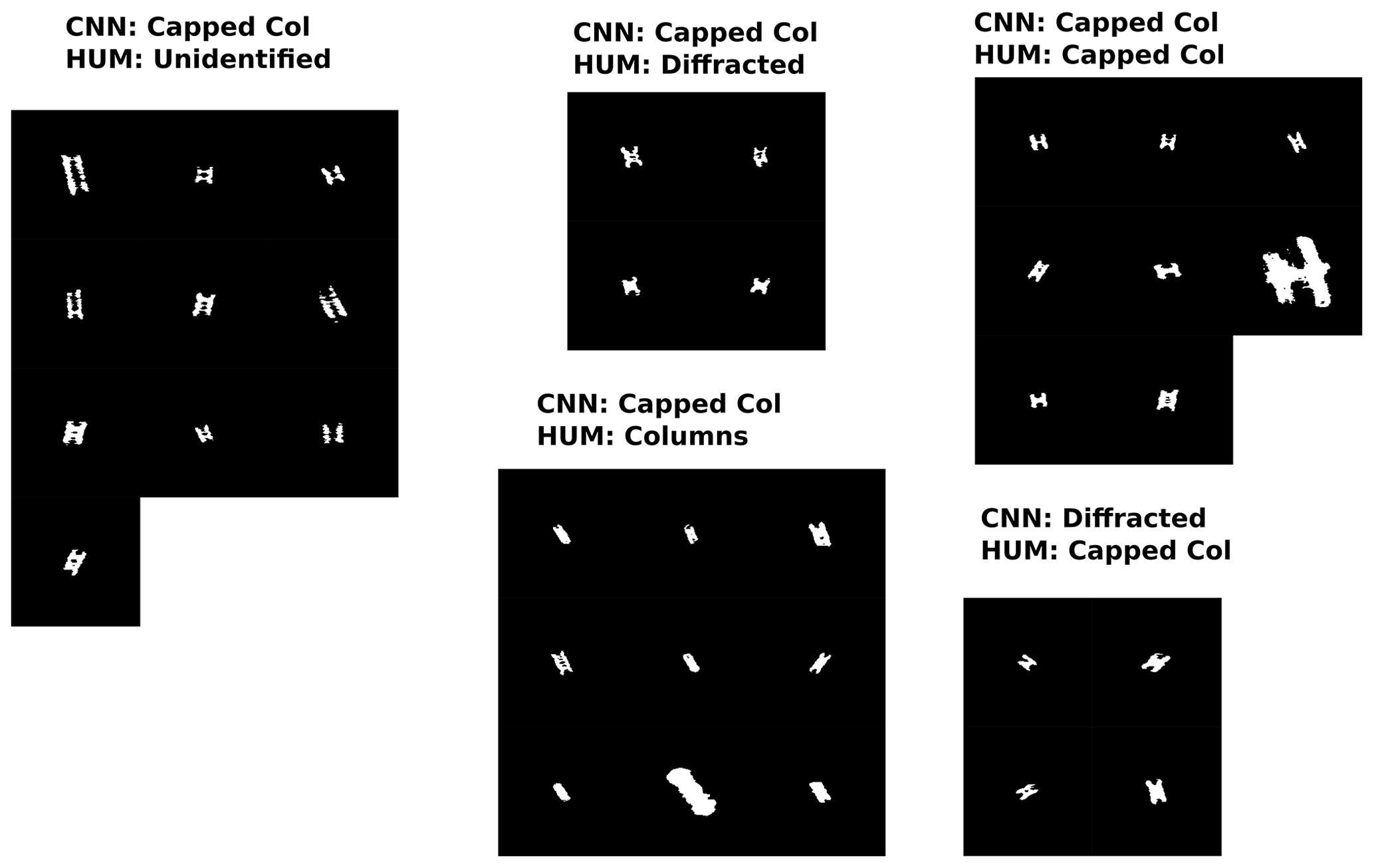
Figure A5Images from the random inspections identified as capped columns by either the CNN or humans.
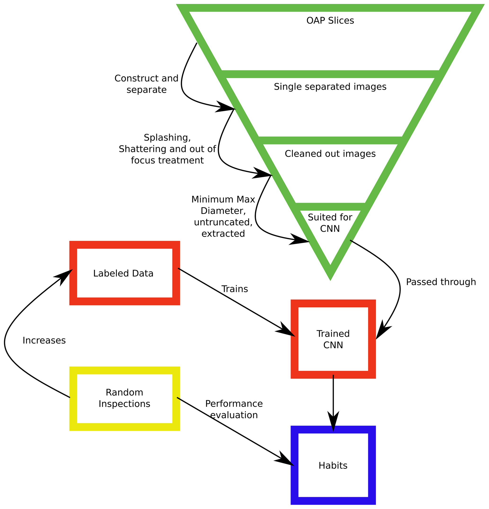
Figure A6Ideal use of the algorithm, which allows for improvements of the training set over time and performance evaluation.
All datasets and python codes are available at https://github.com/Ljaffeux/AMT-2022-72 (last access: 9 September 2022, Jaffeux, 2022).
PC, CD, and AS formulated the project. LJ developed the methodology and wrote the code to implement and perfect the method. LJ organized the random inspections. LJ wrote the article with contributions from PC, AS, and CD.
The contact author has declared that none of the authors has any competing interests.
Publisher's note: Copernicus Publications remains neutral with regard to jurisdictional claims in published maps and institutional affiliations.
The authors would like to thank Angelica Bianco, Céline Planche, Clément Bazantay, Frédéric Tridon, Jean-Luc Barray, Nadège Montoux, Olivier Jourdan, and Laurence Niquet for participating in the random inspections of hydrometeor images. Data used in this study (from past projects EUREC4A, EXAEDRE, ICE GENESIS, and HAIC/HIWC) were mainly obtained using ATR-42 and Falcon 20 research aircraft managed by SAFIRE (French facility for airborne research), thereby operating the cloud in situ instrumental payload from the French INSU/CNRS Airborne Measurement Platform (PMA). Minor data were contributed from the past AFLUX project, which is embedded in the German Transregional Collaborative Research Centre TR 172 (ArctiC Amplification: Climate Relevant Atmospheric and SurfaCe Processes, and Feedback Mechanisms (AC)3). The authors would like to thank the EXAEDRE and ICE GENESIS projects for financing the PhD thesis of Louis Jaffeux.
The French ANR project EXAEDRE was funded by the French Research Ministry (contract no. ANR-16-CE04-0005). The ICE GENESIS project has received support from the European Union's Horizon 2020 research and innovation program (ICE GENESIS project (grant no. 824310)).
This paper was edited by Maximilian Maahn and reviewed by two anonymous referees.
Bailey, M. P. and Hallett, J.: A Comprehensive Habit Diagram for Atmospheric Ice Crystals: Confirmation from the Laboratory, AIRS II, and Other Field Studies, J. Atmos. Sci., 66, 2888–2899, https://doi.org/10.1175/2009JAS2883.1, 2009. a
Baumgardner, D., Avallone, L., Bansemer, A., Borrmann, S., Brown, P., Bundke, U., Chuang, P., Cziczo, D., Field, P., Gallagher, M., and Gayet, J. F.: In situ, airborne instrumentation: Addressing and solving measurement problems in ice clouds, Bull. Am. Meteorol. Soc., 93, p. 9.1, 2012. a
Bony, S., Lothon, M., Delanoë, J., Coutris, P., Etienne, J.-C., Aemisegger, F., Albright, A. L., André, T., Bellec, H., Baron, A., Bourdinot, J.-F., Brilouet, P.-E., Bourdon, A., Canonici, J.-C., Caudoux, C., Chazette, P., Cluzeau, M., Cornet, C., Desbios, J.-P., Duchanoy, D., Flamant, C., Fildier, B., Gourbeyre, C., Guiraud, L., Jiang, T., Lainard, C., Le Gac, C., Lendroit, C., Lernould, J., Perrin, T., Pouvesle, F., Richard, P., Rochetin, N., Salaün, K., Schwarzenboeck, A., Seurat, G., Stevens, B., Totems, J., Touzé-Peiffer, L., Vergez, G., Vial, J., Villiger, L., and Vogel, R.: EUREC4A observations from the SAFIRE ATR42 aircraft, Earth Syst. Sci. Data, 14, 2021–2064, https://doi.org/10.5194/essd-14-2021-2022, 2022. a
Chollet, F., Bursztein, E. Haifeng Jin, H., Matt Watson, M., and Qianli Scott Zhu, Q. S.: Keras, https://github.com/fchollet/keras (last access: 7 September 2022), 2015. a, b
Defer, E., Pinty, J.-P., Coquillat, S., Martin, J.-M., Prieur, S., Soula, S., Richard, E., Rison, W., Krehbiel, P., Thomas, R., Rodeheffer, D., Vergeiner, C., Malaterre, F., Pedeboy, S., Schulz, W., Farges, T., Gallin, L.-J., Ortéga, P., Ribaud, J.-F., Anderson, G., Betz, H.-D., Meneux, B., Kotroni, V., Lagouvardos, K., Roos, S., Ducrocq, V., Roussot, O., Labatut, L., and Molinié, G.: An overview of the lightning and atmospheric electricity observations collected in southern France during the HYdrological cycle in Mediterranean EXperiment (HyMeX), Special Observation Period 1, Atmos. Meas. Tech., 8, 649–669, https://doi.org/10.5194/amt-8-649-2015, 2015. a, b, c
Dezitter, F., Grandin, A., Brenguier, J.-L., Hervy, F., Schlager, H., Villedieu, P., and Zalamansky, G.: HAIC-High Altitude Ice Crystals, in: 5th AIAA Atmospheric and Space Environments Conference, San Diego, United States, 25 June 2013, p. 2674, https://doi.org/10.2514/6.2013-2674, 2013. a, b
Duroure, C.: Une nouvelle méthode de traitement des images d'hydrométéores données par les sondes bidimensionnelles, Journal de recherches atmosphériques, https://hal.uca.fr/hal-01950254 (last access: 7 September 2022), 1982. a
Gao, J., Jiang, Q., Zhou, B., and Chen, D.: Convolutional neural networks for computer-aided detection or diagnosis in medical image analysis: an overview, Math. Biosci. Eng., 16, 6536–6561, 2019. a
Goodfellow, I., Bengio, Y., and Courville, A.: Deep Learning, MIT Press, http://www.deeplearningbook.org (last access: 7 September 2022), 2016. a, b
He, K., Zhang, X., Ren, S., and Sun, J.: Deep Residual Learning for Image Recognition, in: Proceedings of the IEEE Conference on Computer Vision and Pattern Recognition (CVPR), Tours, France, 27–30 June 2016, https://doi.org/10.1109/CVPR.2016.90, 2016. a
Hobbs, P. V., Chang, S., and Locatelli, J. D.: The dimensions and aggregation of ice crystals in natural clouds, J. Geophys. Res., 79, 2199–2206, https://doi.org/10.1029/JC079i015p02199, 1974. a
Houze, R. A., McMurdie, L. A., Petersen, W. A., Schwaller, M. R., Baccus, W., Lundquist, J. D., Mass, C. F., Nijssen, B., Rutledge, S. A., Hudak, D. R., Tanelli, S., Mace, G. G., Poellot, M. R., Lettenmaier, D. P., Zagrodnik, J. P., Rowe, A. K., DeHart, J. C., Madaus, L. E., Barnes, H. C., and Chandrasekar, V.: The Olympic Mountains Experiment (OLYMPEX), Bull. Am. Meteorol. Soc., 98, 2167–2188, https://doi.org/10.1175/BAMS-D-16-0182.1, 2017. a, b
Jaffeux, L.: LJaffeux/AMT-2022-72: Ice crystals images from Optical Array Probes: classification with Convolutional Neural Networks, Zenodo [code and data set], https://doi.org/10.5281/zenodo.6912294, 2022. a
Kikuchi, K., Kameda, T., Higuchi, K., and Yamashita, A.: A global classification of snow crystals, ice crystals, and solid precipitation based on observations from middle latitudes to polar regions, Atmos. Res., 132/133, 460–472, https://doi.org/10.1016/j.atmosres.2013.06.006, 2013. a, b, c
Knollenberg, R. G.: The Optical Array: An Alternative to Scattering or Extinction for Airborne Particle Size Determination, J. Appl. Meteorol., 9, 86–103, https://doi.org/10.1175/1520-0450(1970)009<0086:TOAAAT>2.0.CO;2, 1970. a
Korolev, A. and Sussman, B.: A technique for habit classification of cloud particles, J. Atmos. Ocean. Technol., 17, 1048–1057, 2000. a
Krizhevsky, A., Sutskever, I., and Hinton, G. E.: Imagenet classification with deep convolutional neural networks, Adv. Neur. In., 25, 1097–1105, 2012. a, b
Lawson, R. P., Baker, B. A., Zmarly, P., O'Connor, D., Mo, Q., Gayet, J.-F., and Shcherbakov, V.: Microphysical and optical properties of atmospheric ice crystals at South Pole Station, J. Appl. Meteorol. Clim., 45, 1505–1524, 2006. a
Leinonen, J., Grazioli, J., and Berne, A.: Reconstruction of the mass and geometry of snowfall particles from multi-angle snowflake camera (MASC) images, Atmos. Meas. Tech., 14, 6851–6866, https://doi.org/10.5194/amt-14-6851-2021, 2021. a
Leroy, D., Fontaine, E., Schwarzenboeck, A., Strapp, J. W., Korolev, A., McFarquhar, G. M., Dupuy, R., Gourbeyre, C., Lilie, L., Protat, A., Delanoë, J., Dezitter, F., and Grandin, A.: Ice crystal sizes in high ice water content clouds. Part 2: Statistics of mass diameter percentiles in tropical convection observed during the HAIC/HIWC project, J. Atmos. Ocean. Technol., 34, 117–136, https://doi.org/10.1175/jtech-d-15-0246.1, 2017. a
Lindqvist, H., Muinonen, K., Nousiainen, T., Um, J., McFarquhar, G. M., Haapanala, P., Makkonen, R., and Hakkarainen, H.: Ice-cloud particle habit classification using principal components, J. Geophys. Res.-Atmos., 117, D16, https://doi.org/10.1029/2012JD017573, 2012. a
Luo, J. Y., Irisson, J.-O., Graham, B., Guigand, C., Sarafraz, A., Mader, C., and Cowen, R. K.: Automated plankton image analysis using convolutional neural networks, Limnol. Oceanogr.-Method., 16, 814–827, 2018. a
Magono, C. and Lee, C. W.: Meteorological classification of natural snow crystals, Journal of the Faculty of Science, Hokkaido University, Series 7, Geophysics, 2, 321–335, 1966. a, b, c
McFarquhar, G. M., Ghan, S., Verlinde, J., Korolev, A., Strapp, J. W., Schmid, B., Tomlinson, J. M., Wolde, M., Brooks, S. D., Cziczo, D., Dubey, M. K., Fan, J., Flynn, C., Gultepe, I., Hubbe, J., Gilles, M. K., Laskin, A., Lawson, P., Leaitch, W. R., Liu, P., Liu, X., Lubin, D., Mazzoleni, C., Macdonald, A.-M., Moffet, R. C., Morrison, H., Ovchinnikov, M., Shupe, M. D., Turner, D. D., Xie, S., Zelenyuk, A., Bae, K., Freer, M., and Glen, A.: Indirect and Semi-direct Aerosol Campaign: The Impact of Arctic Aerosols on Clouds, Bull. Am. Meteorol. Soc., 92, 183–201, https://doi.org/10.1175/2010BAMS2935.1, 2011. a
Nakaya, U.: Snow crystal, natural and artificial, Harvard University Press, https://doi.org/10.4159/harvard.9780674182769, 1954. a
Park, S. and Kwak, N.: Analysis on the dropout effect in convolutional neural networks, in: Asian conference on computer vision, 189–204, S pringer International Publishing, https://doi.org/10.1007/978-3-319-54184-6_12, 2016. a
Praz, C., Roulet, Y.-A., and Berne, A.: Solid hydrometeor classification and riming degree estimation from pictures collected with a Multi-Angle Snowflake Camera, Atmos. Meas. Tech., 10, 1335–1357, https://doi.org/10.5194/amt-10-1335-2017, 2017. a
Praz, C., Ding, S., McFarquhar, G. M., and Berne, A.: A Versatile Method for Ice Particle Habit Classification Using Airborne Imaging Probe Data, J. Geophys. Res.-Atmos., 123, 13472–13495, https://doi.org/10.1029/2018JD029163, 2018. a, b, c, d
Pruppacher, H. and Klett, J.: Microphysics of Clouds and Precipitation, Springer Dordrecht, 18, p. 39, https://doi.org/10.1007/978-0-306-48100-0, 2010. a
Przybylo, V., Sulia, K. J., Lebo, Z. J., and Schmitt, C.: Automated Classification of Cloud Particle Imagery through the Use of Convolutional Neural Networks, in: 101st American Meteorological Society Annual Meeting, AMS, 10–15 January 2021, https://ams.confex.com/ams/101ANNUAL/meetingapp.cgi/Paper/377736, last access: 7 September 2021. a
Rahman, M. M., Quincy, E. A., Jacquot, R. G., and Magee, M. J.: Feature Extraction and Selection for Pattern Recognition of Two-Dimensional Hydrometeor Images, J. Appl. Meteorol., 20, 521–535, https://doi.org/10.1175/1520-0450(1981)020<0521:FEASFP>2.0.CO;2, 1981. a, b
Russakovsky, O., Deng, J., Su, H., Krause, J., Satheesh, S., Ma, S., Huang, Z., Karpathy, A., Khosla, A., Bernstein, M., Berg, A. C., and Fei-Fei, L.: ImageNet Large Scale Visual Recognition Challenge, Int. J. Comput. Vis., 115, 211–252, https://doi.org/10.1007/s11263-015-0816-y, 2015. a
Srivastava, N., Hinton, G., Krizhevsky, A., Sutskever, I., and Salakhutdinov, R.: Dropout: A Simple Way to Prevent Neural Networks from Overfitting, J. Mach. Learn. Res., 15, 1929–1958, http://jmlr.org/papers/v15/srivastava14a.html (last access: 7 September 2022), 2014. a
Sukovich, E. M., Kingsmill, D. E., and Yuter, S. E.: Variability of graupel and snow observed in tropical oceanic convection by aircraft during TRMM KWAJEX, J. Appl. Meteorol. Clim., 48, 185–198, 2009. a
Tajbakhsh, N., Shin, J. Y., Gurudu, S. R., Hurst, R. T., Kendall, C. B., Gotway, M. B., and Liang, J.: Convolutional neural networks for medical image analysis: Full training or fine tuning?, IEEE T. Med. Imaging, 35, 1299–1312, 2016. a
Vaillant de Guélis, T., Schwarzenböck, A., Shcherbakov, V., Gourbeyre, C., Laurent, B., Dupuy, R., Coutris, P., and Duroure, C.: Study of the diffraction pattern of cloud particles and the respective responses of optical array probes, Atmos. Meas. Tech., 12, 2513–2529, https://doi.org/10.5194/amt-12-2513-2019, 2019. a, b
Woods, S., Lawson, R. P., Jensen, E., Bui, T., Thornberry, T., Rollins, A., Pfister, L., and Avery, M.: Microphysical properties of tropical tropopause layer cirrus, J. Geophys. Res.-Atmos., 123, 6053–6069, 2018. a
Wyser, K.: Ice crystal habits and solar radiation, Tellus A, 51, 937–950, 1999. a
Xiao, H., Zhang, F., He, Q., Liu, P., Yan, F., Miao, L., and Yang, Z.: Classification of Ice Crystal Habits Observed From Airborne Cloud Particle Imager by Deep Transfer Learning, Earth Space Sci., 6, 1877–1886, https://doi.org/10.1029/2019EA000636, 2019. a
Yi, B., Yang, P., Liu, Q., van Delst, P., Boukabara, S.-A., and Weng, F.: Improvements on the ice cloud modeling capabilities of the Community Radiative Transfer Model, J. Geophys. Res.-Atmos., 121, 13–577, 2016. a
- Abstract
- Introduction
- Data Description (training data)
- CNN methodology
- Random inspections: assessing performance, understanding the results, and improving training data
- Conclusions
- Appendix A
- Code and data availability
- Author contributions
- Competing interests
- Disclaimer
- Acknowledgements
- Financial support
- Review statement
- References