Improving thermodynamic profile retrievals from microwave radiometers by including radio acoustic sounding system (RASS) observations

Thermodynamic profiles are often retrieved from the multi-wavelength brightness temperature observations made by microwave radiometers (MWRs) using regression methods (linear, quadratic approaches), artificial intelligence (neural networks), or physical iterative methods. Regression and neural network methods are tuned to mean conditions derived from a climatological dataset of thermodynamic profiles collected nearby. In contrast, physical iterative retrievals use a radiative transfer model starting from a climatologically reasonable profile of temperature and water vapor, with the model running iteratively until the derived brightness temperatures match those observed by the MWR within a specified uncertainty.

In this study, a physical iterative approach is used to retrieve temperature and humidity profiles from data collected during XPIA (eXperimental Planetary boundary layer Instrument Assessment), a field campaign held from March to May 2015 at NOAA's Boulder Atmospheric Observatory (BAO) facility. During the campaign, several passive and active remote sensing instruments as well as in situ platforms were deployed and evaluated to determine their suitability for the verification and validation of meteorological processes. Among the deployed remote sensing instruments were a multi-channel MWR as well as two radio acoustic sounding systems (RASSs) associated with 915 and 449 MHz wind profiling radars.

In this study the physical iterative approach is tested with different observational inputs: first using data from surface sensors and the MWR in different configurations and then including data from the RASS in the retrieval with the MWR data. These temperature retrievals are assessed against co-located radiosonde profiles. Results show that the combination of the MWR and RASS observations in the retrieval allows for a more accurate characterization of low-level temperature inversions and that these retrieved temperature profiles match the radiosonde observations better than the temperature profiles retrieved from only the MWR in the layer between the surface and 3 km above ground level (a.g.l.). Specifically, in this layer of the atmosphere, both root mean square errors and standard deviations of the difference between radiosonde and retrievals that combine MWR and RASS are improved by mostly 10 %–20 % compared to the configuration that does not include RASS observations. Pearson correlation coefficients are also improved.

A comparison of the temperature physical retrievals to the manufacturer-provided neural network retrievals is provided in Appendix A.

1 Introduction

Monitoring the state of the atmosphere for process understanding and for model verification and validation requires observations from a variety of instruments, each one having its set of advantages and disadvantages. Using several diverse instruments allows one to monitor different aspects of the atmosphere, while combining them in an optimized synergetic approach can improve the accuracy of the information available on the state of the atmosphere.

During the eXperimental Planetary boundary layer Instrumentation Assessment (XPIA) campaign, an experiment sponsored by the U.S. Department of Energy held at the Boulder Atmospheric Observatory (BAO) in spring 2015, several instruments were deployed (Lundquist et al., 2017) with the goal of assessing their capability for measuring atmospheric boundary layer meteorological variables. XPIA investigated novel measurement approaches and quantified uncertainties associated with these measurement methods. While the main interest of the XPIA campaign was on wind and turbulence, measurements of other important atmospheric variables were also collected, including temperature and humidity. Among the deployed instruments were two identical microwave radiometers (MWRs) and two radio acoustic sounding systems (RASS), as well as radiosonde launches.

MWRs are passive sensors, sensitive to atmospheric temperature, humidity, and liquid water path (LWP), that allow for a high temporal observation of the state of the atmosphere, with some advantages and limitations. In order to estimate profiles of temperature and humidity from the observed brightness temperatures (T_b), several methods could be applied such as regressions, neural network retrievals, or physical retrieval methodologies which can include additional information about the atmospheric state in the retrieval process (e.g., Maahn et al., 2020). Microwave radiative transfer models (e.g., Rosenkranz, 1998; Clough et al., 2005) are commonly used to train statistical retrievals, or as forward models used within physical retrieval methods. Advantages of MWRs include their compact design, the relatively high temporal resolution of the measurements (2–3 min), the possibility to observe the vertical structure of both temperature and moisture through the lower part of the troposphere during both clear and cloudy conditions, and their capability to operate in a standalone mode. Disadvantages include limited accuracy in the presence of rain, rather coarse vertical resolution, and the necessity to have a site-specific climatology for retrievals. Other disadvantages include the challenges related to performing accurate calibrations (Küchler et al., 2016, and references within), radio frequency interference (RFI), and the low accuracy on the retrieved LWP, especially for values of LWP less than 20 g m⁻² (Turner, 2007).

RASSs, in comparison, are active instruments that emit a longitudinal acoustic wave upward, causing a local compression and rarefaction of the ambient air. These density variations are tracked by the Doppler radar associated with the RASS, and the speed of the propagating sound wave is measured. The speed of sound is related to the virtual temperature (T_v) (North et al., 1973), and therefore, RASSs are used to remotely measure vertical profiles of virtual temperature in the boundary layer. Being an active instrument, the RASS is in general more accurate than a passive instrument (Bianco et al., 2017), but they also come with their own disadvantages. The main limitations of RASS for temperature measurements are the low temporal resolution (typically a 5 min averaged RASS profile is measured once or twice per hour), their limited altitude coverage, and the noise “pollution” that impacts local communities. Adachi and Hashiguchi (2019) have shown that RASS could use parametric speakers to take advantage of their high directivity and very low side lobes. Nevertheless, the maximum height reached by the RASS is limited by sound attenuation, which is a function of both radar frequency and atmospheric conditions (May and Wilczak, 1993) such as temperature, humidity, and the advection of the propagating sound wave out of the radar's field of view. Therefore, data availability is usually limited to the lowest several kilometers, depending on the frequency of the radar. In addition, wintertime coverage is usually lower than that in summer, due to increased attenuation of the acoustic signal in cooler and drier environments.

To get a better picture of the state of the temperature and moisture structure of the atmosphere, it makes sense to try to combine the information obtained by both MWR and RASS. Integration of different instruments has been and still is a topic of ongoing scientific interest (Han and Westwater, 1995; Stankov et al., 1996; Bianco et al., 2005; Engelbart et al., 2009; Cimini et al., 2020; Turner and Löhnert, 2021, to name some). In this study, the focus is on the combination of the MWR and RASS observations in the retrievals to improve the accuracy of the temperature profiles in the lowest 3 km compared to physical retrieval approaches that do not include the information from RASS measurements. Some studies have used analyses from numerical weather prediction (NWP) models as an additional constraint in these variational retrievals (e.g., Hewison, 2007; Cimini et al., 2006, 2011; Martinet et al., 2020); however, we have elected not to include model data in this study because we wanted to evaluate the impact of the RASS profiles on the retrievals from a purely observational perspective.

This paper is organized as follows: Sect. 2 summarizes the experimental dataset; Sect. 3 introduces the principles of the physical retrieval approaches used to obtain vertical profiles of the desired variables; Sect. 4 produces statistical analysis of the comparison between the different retrieval approaches and radiosonde measurement; finally, conclusions are presented in Sect. 5.

2 XPIA dataset

The data used in our analysis were collected during the XPIA experiment, held in spring 2015 (March–May) at NOAA's BAO site, in Erie, Colorado (40.0451^∘ N, 105.0057^∘ W, elevation 1584 m.s.l.). XPIA was the last experiment conducted at this facility, as after almost 40 years of operations the BAO 300 m tower was demolished at the end of 2016 (Wolfe and Lataitis, 2018). XPIA was designed to assess the capability of different remote sensing instruments for quantifying boundary layer structure and was a preliminary study as many of these same instruments were later deployed, among other campaigns, for the second Wind Forecast Improvement Project WFIP2 (Shaw et al., 2019; Wilczak et al., 2019), which investigated flows in complex terrain for wind energy applications, where they were for example used to study cold air pools (Adler et al., 2021) and gap flow characteristics (Neiman et al., 2019; Banta et al., 2020). The list of the deployed instruments included active and passive remote-sensing devices and in situ instruments mounted on the BAO tower. Data collected during XPIA are publicly available at https://a2e.energy.gov/projects/xpia (last access: 20 January 2022). A detailed description of the XPIA experiment can be found in Lundquist et al. (2017), while a specific look at the accuracy of the instruments used in this study can be found in Bianco et al. (2017).

2.1 MWR measurements

Two identical MWRs (Radiometrics MP-3000A) managed by NOAA (MWR-NOAA) and by the University of Colorado (MWR-CU) were deployed next to each other at the visitor center ∼600 m south of the BAO tower (see Lundquist et al., 2017, for a detailed map of the study area). Prior to the experiment, both MWRs were thoroughly serviced (sensor cleaning, radome replacement, etc.) and calibrated using an external liquid nitrogen target and an internal ambient target. MWRs are passive devices which record the natural microwave emission in the water vapor and oxygen absorption bands from the atmosphere, providing measurements of the brightness temperatures. Both MWRs have 35 channels spanning a range of frequencies, with 21 channels in the lower (22–30 GHz) K-band frequency band, of which 8 channels were used during XPIA (22.234, 22.5, 23.034, 23.834, 25, 26.234, 28, and 30 GHz) and 14 channels in the higher (51–59 GHz) V-band frequency band, all of which were used in XPIA (51.248, 51.76, 52.28, 52.804, 53.336, 53.848, 54.4, 54.94, 55.5, 56.02, 56.66, 57.288, 57.964, and 58.8 GHz). Frequencies in the K-band are more sensitive to water vapor and cloud liquid water, while frequencies in the V-band are sensitive to atmospheric temperature due to the absorption of atmospheric oxygen (Cadeddu et al., 2013). V-band frequencies or channels can also be divided into two categories: the opaque channels, 56.66 GHz and higher, that are more informative in the layer of the atmosphere from the surface to ∼1 km a.g.l., and the transparent channels, 51–56 GHz, that are more informative above 1 km a.g.l. Both MWRs observed at the zenith and at 15 and 165^∘ elevation angles in the north–south plane (referred to as oblique elevation scans and used as their average hereafter; note zenith views have a 90^∘ elevation angle). However, when MWRs are deployed in locations with unobstructed views, oblique scans can be performed down to 5^∘ elevation angles and may provide better temperature profile accuracy in the lowest 0–1 or even 0–2 km a.g.l. layers (Crewell and Löhnert, 2007).

In addition, each MWR was provided with a separate surface sensor to measure pressure, temperature, and relative humidity at the installation level that was ∼2.5 m a.g.l.. Vertical profiles of temperature (T), water vapor density (WVD), and relative humidity (RH) were retrieved in real time during XPIA every 2–3 min using a neural network (NN) approach provided by the manufacturer of the radiometer (Solheim et al., 1998a, b; Ware et al., 2003). Although the physical retrieval configurations used in this study do not exactly match the NN retrieval configurations, a comparison of both physical and neural network retrievals to the radiosonde temperature data is presented in Appendix A.

Both MWRs nominally operated from 9 March to 7 May 2015, although the MWR-NOAA was unavailable between 5–27 April 2015. For the overlapping dates, temperature profiles retrieved from the two MWRs showed very good agreement with less than 0.5 ^∘C bias and 0.994 correlation (Bianco et al., 2017). For this reason, and because the MWR-CU was available for a longer time period, only the MWR-CU (hereafter simply called MWR) is used.

2.2 WPR–RASS measurements

Two NOAA wind profiling radars (WPRs), operating at frequencies of 915 and 449 MHz, were deployed at the visitor center (same location as the MWR) during XPIA. These systems are primarily designed to measure the vertical profile of the horizontal wind vector, but co-located RASSs also enable the observation of profiles of virtual temperature in the lower atmosphere, with different resolutions and height coverage depending on the WPR. Thus, the RASS associated with the 915 MHz WPR (hereafter referred to as RASS 915) measured virtual temperature from 120 to 1618 m with a vertical resolution of 62 m, and the 449 MHz RASS (hereafter referred to as RASS 449) sampled the boundary layer from 217 to 2001 m with a vertical resolution of 105 m. The maximum height reached by the RASS is a function of both radar frequency and atmospheric conditions (May and Wilczak, 1993) and is usually lower for RASS 915 data, as will be shown later in the analysis.

The RASS data were processed using a radio frequency interference (RFI) removal algorithm (performed on the RASS spectra), a consensus algorithm (Strauch et al., 1984) performed on the moment data using a 60 % consensus threshold, a Weber–Wuertz outlier removal algorithm (Weber et al., 1993) performed on the consensus averages, and a RASS range-correction algorithm (Görsdorf and Lehmann, 2000) using an average relative humidity setting of 50 % determined from the available observations.

2.3 BAO data

The BAO 300 m tower was built in 1977 to study the planetary boundary layer (Kaimal and Gaynor, 1983). During XPIA, measurements were collected at the surface (2 m) and at six higher levels (50, 100, 150, 200, 250, and 300 m a.g.l.). Each tower level was equipped with two sonic anemometers on orthogonal booms and one sensor based on a Sensiron SHT75 solid-state sensor to measure temperature and relative humidity with a time resolution of 1 s, and averaged over 5 min. The more accurate temperature and water vapor observations (Horst et al., 2016) at the BAO tower 2 m a.g.l. level are used in the physical retrieval in place of the less accurate MWR surface sensor.

2.4 Radiosonde measurements

Between 9 March and 7 May 2015, while the MWR was operational, radiosondes were launched by the National Center for Atmospheric Research (NCAR) assisted by several students from the University of Colorado over three selected periods, one each in March, April, and May. All radiosondes were Vaisala model RS92. There were a total of 59 launches, mostly four times per day, around 14:00, 18:00, 22:00, and 02:00 UTC (08:00, 12:00, 16:00, and 20:00 local standard time, LST). The first 35 launches, between 9–19 March, were done from the visitor center, while 11 launches between 15–22 April, and 13 launches between 1–4 May were done from the water tank site, ∼1000 m away from the visitor center (see Lundquist et al., 2017, for a detailed map of the study area). The radiosonde measurements included temperature, dew point temperature, and relative humidity to altitudes usually higher than 10 km a.g.l., with measurements every few seconds. As a first step, for additional verification, the radiosonde data from the 59 launches taken between 9 March and 4 May 2015 were compared to the BAO tower measurements, up to 300 m a.g.l.. These observed datasets match very well, with a correlation coefficient of 0.99 and a standard deviation of ∼0.7 ^∘C. However, one radiosonde profile showed a large bias (>5 ^∘C) against all seven levels of BAO temperature measurements and all available T_v measurements from the RASS 915 (eight measurements up to 600 m a.g.l.) and from the RASS 449 (nine measurements up to 1100 m a.g.l.); therefore this particular radiosonde profile was excluded from the statistical analysis. Moreover, while accurate RASS data can be collected during rain, MWR data could be potentially deteriorated due to water deposition on the radome. Therefore, six profiles (three for 13 March and one each on 1, 3, and 4 May) were eliminated from the statistical evaluation. These restrictions lowered the number of total radiosonde launches used in this study to 52.

3 Physical retrievals

One way to combine the active and passive instruments would be to use the RASS observations up to their maximum available height and stitch them with the profiles obtained from a physical iterative method using MWR data. To do this, the moisture contribution to the RASS virtual temperatures could be removed by using either the relative humidity measured by the MWR or by a climatology of the moisture term. However, merging these different profiles could result in artificial jumps at the connecting heights.

Alternatively, a physical retrieval (PR) iterative approach can be used to retrieve vertical profiles of thermodynamic properties from the MWR and RASS observations in a synergistic manner (e.g., Maahn et al., 2020; Turner and Löhnert, 2021). In this case, an optimal estimation-based physical retrieval is initialized with a climatologically reasonable profile of temperature and water vapor and is iteratively repeated until the computed brightness temperatures match those observed by the MWR within the uncertainty of the observed brightness temperatures and the RASS virtual temperatures within their uncertainties (Rodgers, 2000; Turner and Löhnert, 2014; Cimini et al., 2018; Maahn et al., 2020).

3.1 Iterative retrieval technique

For this study, the PR uses the TROPoe retrieval algorithm (formerly AERIoe; Turner and Löhnert, 2014; Turner and Blumberg, 2019; Turner and Löhnert, 2021). This algorithm is able to use radiance data from microwave radiometers, infrared spectrometers, and other observations as input. The microwave radiative transfer model, MonoRTM (Clough et al., 2005), serves as the forward model, which is fully functional for the microwave region and was intensively evaluated previously on MWR measurements (Payne et al., 2008; 2011).

We start with the state vector X_a= [T, Q, LWP]^T, where superscript T denotes transpose, and vectors and matrices are shown in bold. T (K) and Q (g kg⁻¹) are temperature and water vapor mixing ratio profiles at 55 vertical levels from the surface up to 17 km, with the distance between the levels increasing geometrically with height. LWP is the liquid water path in g m⁻² that measures the integrated content of liquid water in the entire vertical column above the MWR and is a scalar. For this study, X_a has dimensions equal to 111×1 (two vectors T and Q with 55 levels each, and LWP). The retrieval framework of Turner and Blumberg (2019) is used, but only using MWR data (no spectral infrared). Here, we demonstrate the extension of the retrieval to include RASS profiles of T_v and the resulting impact this has on the retrieved temperature profiles and information content.

The observation vector Y includes temperature and water vapor mixing ratio measured at the surface in situ and spectral T_b measured by the MWR. The MonoRTM model F is used as the forward model from the current state vector X and is then compared to the observation vector Y, iterating until the difference between F(X) and Y is small within a specified uncertainty (Eq. 1).

$$\begin{array}{}\text{(1)}& \begin{array}{rl}{\mathit{X}}_{n+\mathrm{1}}={\mathit{X}}_n& +({\mathbf{S}}_a^{-\mathrm{1}}+{\mathbf{K}}^{\mathrm{T}}{\mathbf{S}}_{\mathit{\epsilon }}^{-\mathrm{1}}\mathbf{K}{)}^{-\mathrm{1}}{\mathbf{K}}^{\mathrm{T}}{\mathbf{S}}_{\mathit{\epsilon }}^{-\mathrm{1}}[\mathit{Y}-\mathit{F}\left({\mathit{X}}_n\right)\\ & +\mathbf{K}({\mathit{X}}_n-{\mathit{X}}_a)]\end{array}\end{array}$$

with

$$\begin{array}{rl}{\mathit{X}}_a& =\left[\begin{array}{c}\mathit{T}\\ \mathit{Q}\\ \mathrm{LWP}\end{array}\right]\\ {\mathbf{S}}_a& =\left[\begin{array}{ccc}{\mathit{\sigma }}_{\mathit{T}\mathit{T}}^{\mathrm{2}}& {\mathit{\sigma }}_{\mathit{T}\mathit{Q}}^{\mathrm{2}}& \mathrm{0}\\ {\mathit{\sigma }}_{\mathit{Q}\mathit{T}}^{\mathrm{2}}& {\mathit{\sigma }}_{\mathit{Q}\mathit{Q}}^{\mathrm{2}}& \mathrm{0}\\ \mathrm{0}& \mathrm{0}& {\mathit{\sigma }}_{\mathrm{LWP}}^{\mathrm{2}}\end{array}\right]\\ {\mathbf{K}}_{ij}& ={\displaystyle \frac{\mathbf{\partial }{\mathit{F}}_{\mathit{i}}}{\mathbf{\partial }{\mathit{X}}_{\mathit{j}}}},\end{array}$$

where i and j in the K_ij definition mark channel and vertical level, respectively. The superscripts T and ⁻¹ in Eq. (1) indicate the transpose and inverse matrices, respectively. The observation vector Y and the covariance matrix of the observed data, S_ε, depending on the configuration used, are equal to the following.

$${\displaystyle }\begin{array}{rl}{\mathit{Y}}_{\mathrm{1}}& =\left[\begin{array}{l}{T}_{\mathrm{sfc}}\\ Q_{\mathrm{sfc}}\\ {{\mathit{T}}_{\mathrm{b}}}_{\mathrm{zenith}}\end{array}\right]\\ {\mathbf{S}}_{{\mathit{\epsilon }}_{\mathrm{1}}}& =\left[\begin{array}{ccc}{\mathit{\sigma }}_{T_{\mathrm{sfc}}}^{\mathrm{2}}& \mathrm{0}& \mathrm{0}\\ \mathrm{0}& {\mathit{\sigma }}_{Q_{\mathrm{sfc}}}^{\mathrm{2}}& \mathrm{0}\\ \mathrm{0}& \mathrm{0}& {\mathit{\sigma }}_{{{\mathit{T}}_{\mathrm{b}}}_{\mathrm{zenith}}}^{\mathrm{2}}\end{array}\right]\\ \\ {\mathit{Y}}_{\mathrm{2}}& =\left[\begin{array}{l}{T}_{\mathrm{sfc}}\\ Q_{\mathrm{sfc}}\\ {{\mathit{T}}_{\mathrm{b}}}_{\mathrm{zenith}+\mathrm{oblique}}\end{array}\right]\\ {\mathbf{S}}_{{\mathit{\epsilon }}_{\mathrm{2}}}& =\left[\begin{array}{ccc}{\mathit{\sigma }}_{T_{\mathrm{sfc}}}^{\mathrm{2}}& \mathrm{0}& \mathrm{0}\\ \mathrm{0}& {\mathit{\sigma }}_{Q_{\mathrm{sfc}}}^{\mathrm{2}}& \mathrm{0}\\ \mathrm{0}& \mathrm{0}& {\mathit{\sigma }}_{{{\mathit{T}}_{\mathrm{b}}}_{\mathrm{zenith}+\mathrm{oblique}}}^{\mathrm{2}}\end{array}\right]\\ \\ {\mathit{Y}}_{\mathrm{3}}& =\left[\begin{array}{l}{T}_{\mathrm{sfc}}\\ Q_{\mathrm{sfc}}\\ {{\mathit{T}}_{\mathrm{b}}}_{\mathrm{zenith}+\mathrm{oblique}}\\ {{\mathit{T}}_{\mathrm{v}}}_{\mathrm{RASS}\mathrm{915}}\end{array}\right]\\ {\mathbf{S}}_{{\mathit{\epsilon }}_{\mathrm{3}}}& =\left[\begin{array}{cccc}{\mathit{\sigma }}_{T_{\mathrm{sfc}}}^{\mathrm{2}}& \mathrm{0}& \mathrm{0}& \mathrm{0}\\ \mathrm{0}& {\mathit{\sigma }}_{Q_{\mathrm{sfc}}}^{\mathrm{2}}& \mathrm{0}& \mathrm{0}\\ \mathrm{0}& \mathrm{0}& {\mathit{\sigma }}_{{{\mathit{T}}_{\mathrm{b}}}_{\mathrm{zenith}+\mathrm{oblique}}}^{\mathrm{2}}& \mathrm{0}\\ \mathrm{0}& \mathrm{0}& \mathrm{0}& {\mathit{\sigma }}_{{{\mathit{T}}_{\mathrm{v}}}_{\mathrm{RASS}\mathrm{915}}}^{\mathrm{2}}\end{array}\right]\end{array}$$

$${\displaystyle }\begin{array}{rl}& {\mathit{Y}}_{\mathrm{4}}=\left[\begin{array}{l}{T}_{\mathrm{sfc}}\\ Q_{\mathrm{sfc}}\\ {{\mathit{T}}_{\mathrm{b}}}_{\mathrm{zenith}+\mathrm{oblique}}\\ {{\mathit{T}}_{\mathrm{v}}}_{\mathrm{RASS}\mathrm{449}}\end{array}\right]\\ & {\mathbf{S}}_{{\mathit{\epsilon }}_{\mathrm{4}}}=\left[\begin{array}{cccc}{\mathit{\sigma }}_{T_{\mathrm{sfc}}}^{\mathrm{2}}& \mathrm{0}& \mathrm{0}& \mathrm{0}\\ \mathrm{0}& {\mathit{\sigma }}_{Q_{\mathrm{sfc}}}^{\mathrm{2}}& \mathrm{0}& \mathrm{0}\\ \mathrm{0}& \mathrm{0}& {\mathit{\sigma }}_{{{\mathit{T}}_{\mathrm{b}}}_{\mathrm{zenith}+\mathrm{oblique}}}^{\mathrm{2}}& \mathrm{0}\\ \mathrm{0}& \mathrm{0}& \mathrm{0}& {\mathit{\sigma }}_{{{\mathit{T}}_{\mathrm{v}}}_{\mathrm{RASS}\mathrm{449}}}^{\mathrm{2}}\end{array}\right]\end{array}$$

Note that the 2 m surface-level observations of temperature and water vapor mixing ratio (T_sfc and Q_sfc, respectively) are included as part of the observation vector Y, and thus the uncertainties (0.5 K for temperature and less than 0.4 g kg⁻¹ for mixing ratio) in these observations are included in S_ε.

The mean state vector of the climatological estimates, or a “prior” vector X_a, is a key component in the optimal estimation framework, and it is the first guess of the state vector X, X₁, in Eq. (1). It provides a constraint on the ill-posed inversion problem. The prior is calculated independently for each month of the year from climatological sounding profiles (using 10 years of data) in the Denver area. The covariance matrix, S_a, of the “prior” vector includes not only temperature or water vapor variances but also the covariances between them. Using around 3000 radiosondes launched by the NWS in Denver, each radiosonde profile is interpolated to the vertical levels used in the retrieval, after which the covariance of temperature and temperature, temperature and humidity, and humidity and humidity is computed for different levels. LWP is arbitrarily assigned in X_a, with large values chosen for its uncertainty in S_a, so that it does not impact (constrain) the retrieval. Presently, the assumed uncertainty in LWP in the prior is assigned to 200 g m⁻² in the TROPoe configuration file.

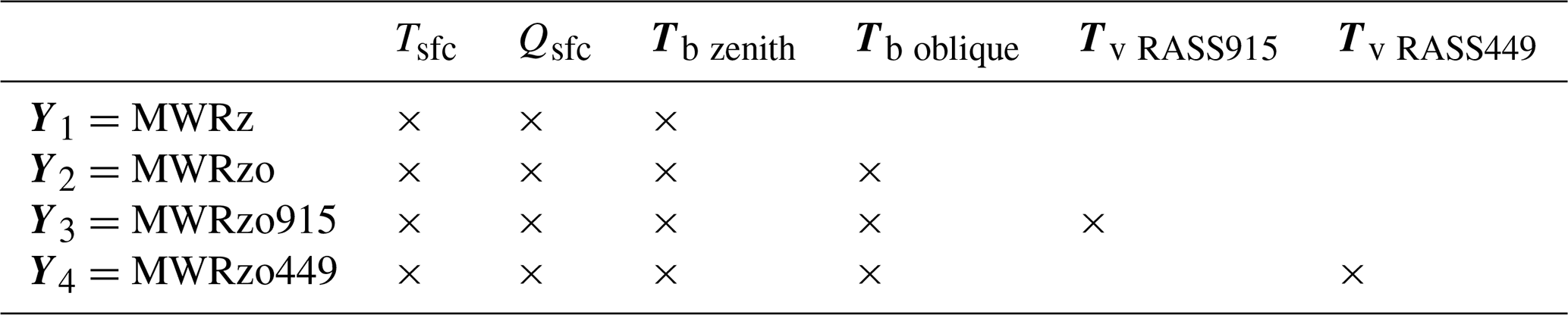
Four configurations are chosen for the observational vector Y (Y₁, Y₂, Y₃, and Y₄). In each of these, the surface observations are obtained by the 2 m BAO in situ measurements of temperature and humidity. The MWR provides T_b measurements from 22 channels from the zenith scan for the zenith-only configuration (Y₁), while when using the zenith plus oblique T_b inputs (Y₂, Y₃, and Y₄) the same 22 channels were used from the zenith scans together with only the four opaque channels (56.66, 57.288, 57.964, and 58.8 GHz) from the oblique scans. Using additional measurements from the co-located radar systems with RASS, the observational vector is further expanded with either RASS 915 (Y₃) or RASS 449 (Y₄) virtual temperature observations. The covariance matrix of the observed data, S_ε, depends on the chosen Y_i as seen in the matrix S_εi (with $i=\mathrm{1}:\mathrm{4}$) descriptions, with increasing dimensions from Y₁ to Y₂ and additional increasing dimensions to Y₃ or Y₄ through the multi-level measurements of the RASS (Turner and Blumberg, 2019). Table 1 summarizes the observational information included in these four different configurations of the PR.

Table 1 Four PR configurations corresponding to the four observational Y_i vectors in Eq. (1).

The uncertainty in the MWR T_b observations was set to the standard deviation from a detrended time-series analysis for each channel during cloud-free periods. The method to detect those cloud-free periods is described in detail in Sect. 3.2. The derived uncertainties ranged from 0.3 to 0.4 K in the 22 to 30 GHz channels and 0.4 to 0.8 K in the 52 to 60 GHz channels. We assumed that there was no correlated error between the different MWR channels.

For the RASS, co-located RASS and radiosonde profiles were compared, and the standard deviation of the differences in T_v was determined as a function of the radar's signal-to-noise ratio (SNR). This relationship resulted in uncertainties that ranged from 0.8 at high SNR values to 1.5 K at low SNR values. Again, we assumed that there was no correlated error between different RASS heights. Following these assumptions, the covariance matrix S_ε is diagonal.

The Jacobian matrix, K, is computed using finite differences by perturbing the elements of X and rerunning the forward model. It has dimensions m×111, where m is the length of the vector Y_i; therefore its dimension increases correspondingly with the inclusion of more observational data. K makes the “connection” between the state vector and the observational data and should be calculated at every iteration.

3.2 Bias correction of MWR observations using radiosondes or climatology

Observational errors propagate through retrieval into the derived profiles (i.e., the bias of the observed data will contribute to a bias in the retrievals). For that, retrieval uncertainties in Eq. (1) from Y=Y₁ or Y₂ derive only from uncertainties in surface and MWR data, while retrieval uncertainties from Y=Y₃ or Y₄ come from uncertainties in the surface, MWR, and RASS measurements.

The bias of the retrieval depends on both the absolute accuracy of the forward model and on any observational systematic offset, of which the systematic error in the MWR observations could potentially be reduced through application of an MWR T_b bias-correction procedure. In this study, two different approaches were used for the bias correction: the first is based on a comparison to the radiosondes, while the second uses climatological profiles. The first method could be used for a field campaign where occasional co-located radiosonde launches are taken, while the second would be used for deployments without any supporting radiosonde observations.

For both approaches, the first step is to identify clear-sky periods during which the bias can be estimated (to eliminate uncertainties associated with clouds), and subsequently the bias can be removed from the observed MWR T_bs. One method to identify clear-sky times is to use a time series of T_b observations in the 30 GHz liquid-water-sensitive channel of the MWR.

The standard deviation of the MWR T_b in the 30 GHz channel is calculated over a time frame of 1 h centered at the radiosonde launch time. The data from the zenith scan and the averaged oblique scans are reviewed separately. Liquid-cloud-free periods were identified by cases where the temporal standard deviation was small (<0.4 K), and more than 35 radiosonde profiles were classified as being launched in clear skies. The usage of the standard deviation from the time series from the oblique scans, with the same 0.4 K restriction, reduces the number of the clear-sky radiosonde profiles to 18. For those chosen 18 radiosonde profiles, the T_b is calculated from radiosonde temperature profiles through MonoRTM at each of the MWR channels. The mean difference between these calculated radiosonde T_bs and measured MWR T_bs forms the T_b bias with which the MWR T_b data can be corrected. This bias-correction method will be referred to as “radiosonde BC”.

While this radiosonde BC method can be employed for the XPIA dataset, for other campaigns this approach would not be possible if co-located radiosonde observations were not available. For this situation, an alternative method for correcting the MWR T_b biases is presented. There are often spectral features in the observed minus computed brightness temperature residuals that could not be explained by any physically realistic atmospheric profiles and can only result because of a calibration error in the observations. This alternative bias-correction method is aimed purely to remove this unphysical spectral signature. In this method, to choose clear-sky periods, the 30 GHz channel MWR T_b data are used on a daily basis. The standard deviation of the MWR T_b is calculated as the average of standard deviations in a 1 h sliding window through all data points of a day. Four clear-sky days were identified using a threshold of 0.4 K on the standard deviation: 10 and 30 March and 13 and 29 April 2015. The T_b bias is then computed for each of the 22 channels as the averaged difference between the observed T_b from the MWR zenith observations and the forward-model-calculated T_b values at zenith using the TROPoe-retrieved profiles (Y₁) of those selected clear-sky days. This method identified spectral calibration errors in the MWR observations that could not be explained by physically realistic atmospheric profiles. This bias-correction technique, which accounts for those unphysical spectral calibration features, will be referred to as “TROPoe BC”.

Figure 1 shows the T_b biases found for all 22 MWR channels from both bias-correction approaches. The biases calculated with the radiosonde BC scheme are shown for all channels used in our analysis: 22 channels of the zenith scan, in red, and four V-band opaque channels of the oblique scans, in blue. The black and green triangles represent the biases calculated using the TROPoe BC approach for zenith and for zenith+oblique scans, respectively. All biases are presented with associated uncertainties (error bars representing the standard deviation over all radiosondes for radiosonde BC and mean observation T_b vector uncertainties for 4 chosen clear-sky days for TROPoe BC).

Figure 1 T_b biases derived from the radiosonde BC method (and TROPoe BC method) in all 22 MWR channels of the zenith scan in red (and in black) and in the four opaque channels of the oblique scans in blue (and in green).

The biases from the two bias-correction schemes are within the uncertainties of each other for most of the channels except at the higher frequencies in the V-band. Biases in the most opaque channels are significantly affected by the accuracy of the boundary layer temperature profiles. When TROPoe BC is used, a monthly average prior temperature profile is used in the PR and thus differences between this prior profile and the actual temperature profile can result in a spectral bias in the more opaque MWR channels. On the contrary, the radiosonde BC uses a direct measurement of the temperature profile (from the radiosonde), and thus is more accurate. It is also important to note that, in both approaches, the biases in the opaque channels for zenith and for oblique scans (for radiosonde BC these are red and blue, respectively, and for the TROPoe BC these are black and green, respectively) are very similar to each other. This supports the assumption that the true bias is nearly independent of the scene, or that the sensitivity to the scene (e.g., zenith or off-zenith) is small.

The bias-correction methods were applied by removing the corresponding calculated biases from the MWR T_b observations before the retrievals were performed. Later in Sect. 4, differences in the retrieved temperature profiles will be shown when using the two bias-correction approaches. These differences will be more evident in the temperature profiles exhibiting near-ground temperature inversions.

However, the final goal of this study is not to assess the sensitivity to different bias-correction approaches but to verify that the inclusion of RASS observations does improve retrieved temperature profiles, independently of the bias-correction method used.

3.3 Analysis of physical retrieval characteristics

The retrieved profiles of the four different PR configurations presented in Table 1 (MWRz, MWRzo, MWRzo915, MWRzo449) were compared to the radiosonde profiles. To compare radiosonde observations against the PR profiles, all radiosonde profiles were interpolated vertically to the same PR heights, and PR profiles were averaged in the time window between 15 min before and 15 min after each radiosonde launch. Since the radiosonde ascends quite quickly in the lowest kilometers of the atmosphere (∼15–20 min to reach 5 km), the 30 min temporal window is estimated to be representative of the same volume of the atmosphere measured by the radiosonde. BAO tower temperature and mixing ratio data at the seven available levels were used as an additional validation dataset, without any vertical interpolation, averaged in the time window between 15 min before and 15 min after each radiosonde launch.

As an example of the different temperature retrievals and their relative performance, data obtained on 17 March 2015 at 22:00 UTC are presented in Fig. 2. Temperature profiles up to 2 km a.g.l. retrieved from the four PR configurations (MWRz, MWRzo, MWRzo915, MWRzo449, using the radiosonde BC) are compared to the radiosonde data in red and to the BAO measurements in blue squares. Note that all four of the PRs match the BAO observations reasonably well near the ground. The MWRz and MWRzo profiles are very smooth and depart quite substantially from the radiosonde measurements and are unable to reproduce the more detailed structure of the atmospheric temperature profile measured by the radiosonde, while the MWRzo449 profile (in light blue) demonstrates a better agreement with both the radiosonde and BAO measurements (blue squares). The MWRzo915 profile (in magenta) also tries to follow the elevated temperature inversion observed by the radiosonde, successful only in the lower part of the atmosphere (below 1 km a.g.l.) where RASS 915 measurements are available. This behavior will also be addressed in the following section and in the statistical analysis presented later in the paper.

Figure 2 Temperature profiles obtained by the four PR configurations, after applying the radiosonde BC to the MWR T_bs: MWRz in gray, MWRzo in black, MWRzo915 in magenta, and MWRzo449 in light blue. These retrievals are compared to radiosonde measurements, in red, and BAO tower observations, as blue squares. The heights with available RASS virtual temperature measurements (RASS 915 in magenta and RASS 449 in light blue) are marked by the asterisks on the right y axis.

An asset of TROPoe is that several characteristics of the PRs can be obtained from two matrices, the averaging kernel, Akernel, and the posterior covariance matrix, S_op (Masiello et al., 2012; Turner and Löhnert, 2014, Turner and Bloomberg, 2019), calculated as

$$\begin{array}{}\text{(2)}& \mathbf{Akernel}={\mathbf{B}}^{-\mathrm{1}}{\mathbf{K}}^T{\mathbf{S}}_{\mathit{\epsilon }}^{-\mathrm{1}}\mathbf{K}\end{array}$$

and

$$\begin{array}{}\text{(3)}& {\mathbf{S}}_{\mathrm{op}}={\mathbf{B}}^{-\mathrm{1}},\end{array}$$

where

$$\mathbf{B}={\mathbf{S}}_a^{-\mathrm{1}}+{\mathbf{K}}^T{\mathbf{S}}_{\mathit{\epsilon }}^{-\mathrm{1}}\mathbf{K}.$$

All matrices, Akernel, S_op, and B, have dimensions 111×111 in our configuration. While the top left corner of the Akernel matrix (1:55, 1:55) is devoted to temperature, called ATkernel in the text, the next (56:110, 56:110) elements are devoted to the water vapor mixing ratio, called AQKernel.

The Akernel provides useful information about the calculated retrievals, such as vertical resolution and degrees of freedom for signal at each level. The rows of the Akernel provide the smoothing functions (Rodgers, 2000) that could be applied to the radiosonde profiles (Eq. 4) to minimize the vertical representativeness error in the comparison between the various retrievals and the radiosonde profiles due to very different vertical resolutions of these profiles (Turner and Löhnert, 2014).

Smoothed radiosonde observed profiles can be computed using the averaging kernel as

$$\begin{array}{}\text{(4)}& {\mathit{X}}_{{\mathrm{smoothed}}_{\mathrm{radiosonde}}}=\mathbf{Akernel}({\mathit{X}}_{\mathrm{radiosonde}}-{\mathit{X}}_a)+{\mathit{X}}_a.\end{array}$$

The Akernel in Eq. (2) depends on the retrieval parameters (e.g., which datasets are used in the Y vector, the values assumed in the observation covariance matrix S_ε, and the sensitivity of the forward model), so for our four PR configurations it is possible to calculate four different kernels from Eq. (2).

For each of the four Akernels, a smoothed radiosonde profile can be computed for each radiosonde profile using Eq. (4). In the presence of temperature inversions or other particular structures in the atmosphere, these smoothed profiles can be quite different from each other and also from the original unsmoothed radiosonde profile. Consequently, while comparison of the retrievals to the relative Akernel-smoothed radiosonde profiles can be used to minimize the vertical representativeness effects due to the different vertical resolutions of these profiles, we note that a statistical comparison between the four configurations of the observational vector would not be fair if each of their retrieved profiles is compared to a different Akernel-smoothed radiosonde profile. Therefore, in the statistical analysis presented later in the paper (Sect. 4.2), mean bias, root-mean-square error (RMSE), and Pearson correlation coefficients will be computed between the various TROPoe retrieval configurations and the unsmoothed radiosonde profiles, just interpolated to the same vertical levels of the retrieved profiles.

The ATkernel can help understand the differences in the retrieved temperature profiles obtained by the configurations using additional RASS data, shown in the example of Fig. 2. Figure 3a includes the temperature profiles of the radiosonde (unsmoothed and ATkernel's smoothed) and PRs of MWRzo and MWRzo449 for the same example as in Fig. 2. Due to the inclusion of RASS measurements, the ATkernel-smoothed radiosonde profile of the MWRzo449 configuration (dashed light blue line) is closer to the original radiosonde data (in red) compared to the black dashed profile of the MWRzo's ATkernel-smoothed radiosonde profile. Additionally, the rows of the ATkernel provide a measure of the retrieval smoothing as a function of altitude, so the full width at half maximum (FWHM) of each ATkernel row estimates the vertical resolution of the retrieved solution at each vertical level (Maddy and Barnet, 2008; Merrelli and Turner, 2012). Plots of this vertical resolution as a function of the height for the MWRzo PR and for the MWRzo449 PR are included in Fig. 3b. This plot shows that the additional observations from the RASS 449 significantly improve the vertical resolution of the retrievals.

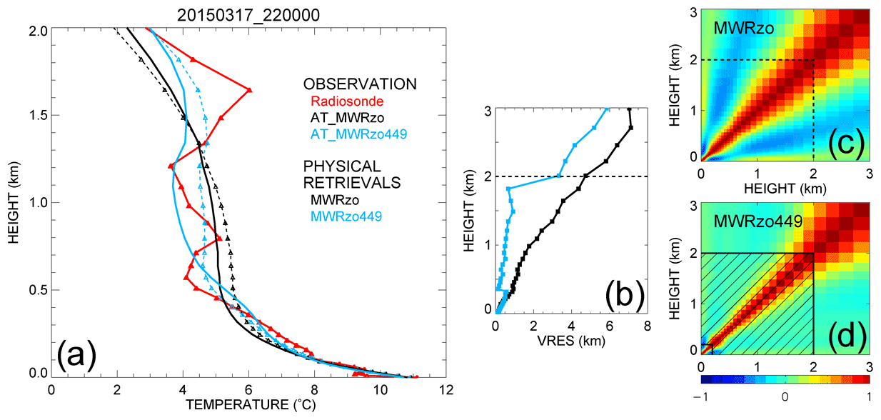
Figure 3 (a) Observed temperature profiles from radiosonde in red, from ATkernel-smoothed radiosonde, AT_MWRzo in dashed black, and AT_MWRzo449 in dashed light blue; PRs from MWRzo PR in solid black, and from MWRzo449 PR in solid light blue. (b) Vertical resolution (VRES) as a function of the height for the MWRzo PR (black) and for the MWRzo449 PR (light blue). (c, d) 3×3 km (37×37 levels) S_op matrices, converted to correlation matrices, for the MWRzo PR (c) and for the MWRzo449 PR (d). Dashed lines on plots (b–d) mark 2 km a.g.l. Hatched area on panel (d) marks the RASS measurement heights.

The posterior covariance matrix, S_op, provides a measure of the uncertainty of the retrievals while the square root of the diagonal of this matrix is used to specify the 1σ errors in the profiles of temperature or mixing ratio. Also, S_op shows the level-to-level dependency of the retrievals and in an ideal case should have all non-diagonal elements equal to zero. Converted to a correlation matrix, it is possible to visualize these dependencies, as presented in Fig. 3c, d. The use of additional RASS data (MWRzo449 S_op, Fig. 3d) reduces the off-diagonal covariances, therefore substantially decreasing the correlations in those areas compared to the MWRzo S_op (Fig. 3c).

To understand the level-to-level correlations among the four different retrieval configurations in Table 1, the S_op matrices were averaged over all radiosonde events and converted to correlation matrices (Fig. 4). A clearly visible narrowing of the spread around the main diagonal and correlation reduction in the off-diagonal elements results by adding additional observations, from MWR zenith only (Fig. 4a), to MWR zenith-oblique (Fig. 4b), to the larger impact obtained by the usage of the RASS 915 (Fig. 4c), concluding with the RASS 449 (Fig. 4d) data. The mean retrieval uncertainty profile for each of the PR configurations is presented in Fig. 4e. The uncertainty of the MWRzo449 retrieval up to 1 km a.g.l. is around 0.5 ^∘C while the other retrievals have higher uncertainties of up to 1 ^∘C. The higher accuracy of the MWRzo449 retrievals is because that configuration has more observational information compared to the other retrieval configurations.

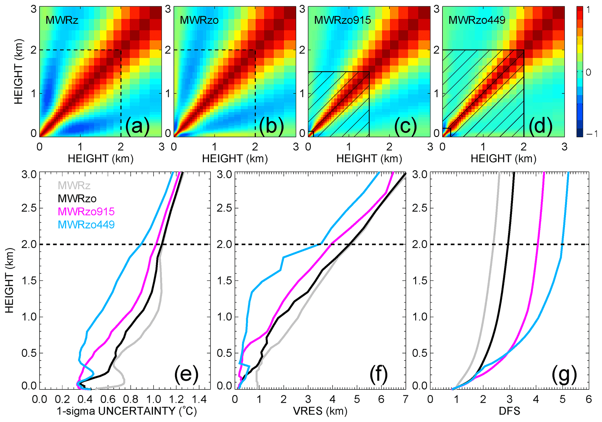
Figure 4 (a–d) The mean S_ops, displayed as correlation matrices, for (a) MWRz, (b) MWRzo, (c) MWRzo915, and (d) MWRzo449, averaged over all radiosonde events. The hatched area in panels (c) and (d) marks the RASS maximum measurement heights. (e) One-sigma uncertainty derived from the posterior covariance matrix in ^∘C, (f) vertical resolution (VRES) in kilometers, and (g) cumulative degree of freedom (DFS) as a function of height for temperature, averaged over all radiosonde events (MWRz is in gray, MWRzo is in black, MWRzo915 is in magenta, and MWRzo449 is in light blue). Dashed lines mark 2 km a.g.l. in all panels.

Other statistically important features to analyze in the PRs, besides their uncertainty, are the vertical resolution already introduced in the example of Fig. 3b and the degree of freedom for signal (DFS). These two features, derived from the Akernels of each PR configuration, averaged over all radiosonde events, are shown in Fig. 4f and g. The vertical resolution (Fig. 4f) shows the width of the atmosphere layer used for each retrieval height, computed as the full width at half maximum value of the averaging kernel. The cumulative DFS profile (Fig. 4g) is a measure of the number of independent pieces of information in the observations below the specified height. For example, at the 1 km a.g.l. level the vertical resolution of MWRzo449 is 0.5 km (i.e., information from ±0.5 km around the retrieval height is considered in the retrieval), while all other retrievals use the information from more than ±1.5 km. Also, the DFS, as a cumulative measure, shows an increase in pieces of information from MWRz to MWRzo for the whole profile and from MWRzo to MWRzo915 and to MWRzo449 above ∼0.2 km where RASS data are available. The DFS of MWRzo915 is higher compared to the DFS of MWRzo449 in the 0.2–0.5 km a.g.l. layer because RASS 915 data have denser measurements there. It is also important to note that there is no additional information added to any of the retrievals above 2 km a.g.l.; i.e., the slope of the cumulative DFS profiles are equal. Despite that, the statistical analysis of the PRs up to 3 km a.g.l., shown in Sect. 4, will prove that the retrieval improvements obtained by including the RASS are found even above the height of the RASS measurement availability.

The improvements from MWRz (in gray) to MWRzo (in black), to MWRzo915 (in magenta), and finally to MWRzo449 (in light blue) are visible in all three panels (Fig. 4e–g), whereas MWRzo449 has the lowest 1σ uncertainty and highest DFS compared to the other PRs, particularly below 2 km a.g.l., where RASS 449 measurements are available. Finally, it is interesting that below 200 m a.g.l. the MWRzo915 has slightly smaller lowest 1σ uncertainty and vertical resolution relative to the MWRzo449, as could be expected due to the first available height of the RASS 915 being lower (120 m a.g.l.) than the first available height for the RASS 449 (217 m a.g.l.) and due to the finer vertical resolution of the 915 MHz RASS. This suggests that, if additional observations were available in the lowest several hundred meters of the atmosphere where RASS measurements are not available, improvements might be even better closer to the surface, where temperature inversions, if present, are sometimes difficult to retrieve correctly.

4 Results

4.1 Statistical analysis of physical retrievals up to 3 km a.g.l.

Several cases were found during XPIA when the temperature profile exhibited inversions, with the lowest happening in the surface layer. Figure 5 shows one of the most complex cases, with several temperature inversions visible in the temperature profile from the radiosonde (red line), in the temperature measurements from the BAO tower (blue squares), and in the virtual temperature measured by the RASS 449 (light blue triangles). Note that the virtual temperature profile is in close agreement with the temperature measured by radiosonde.

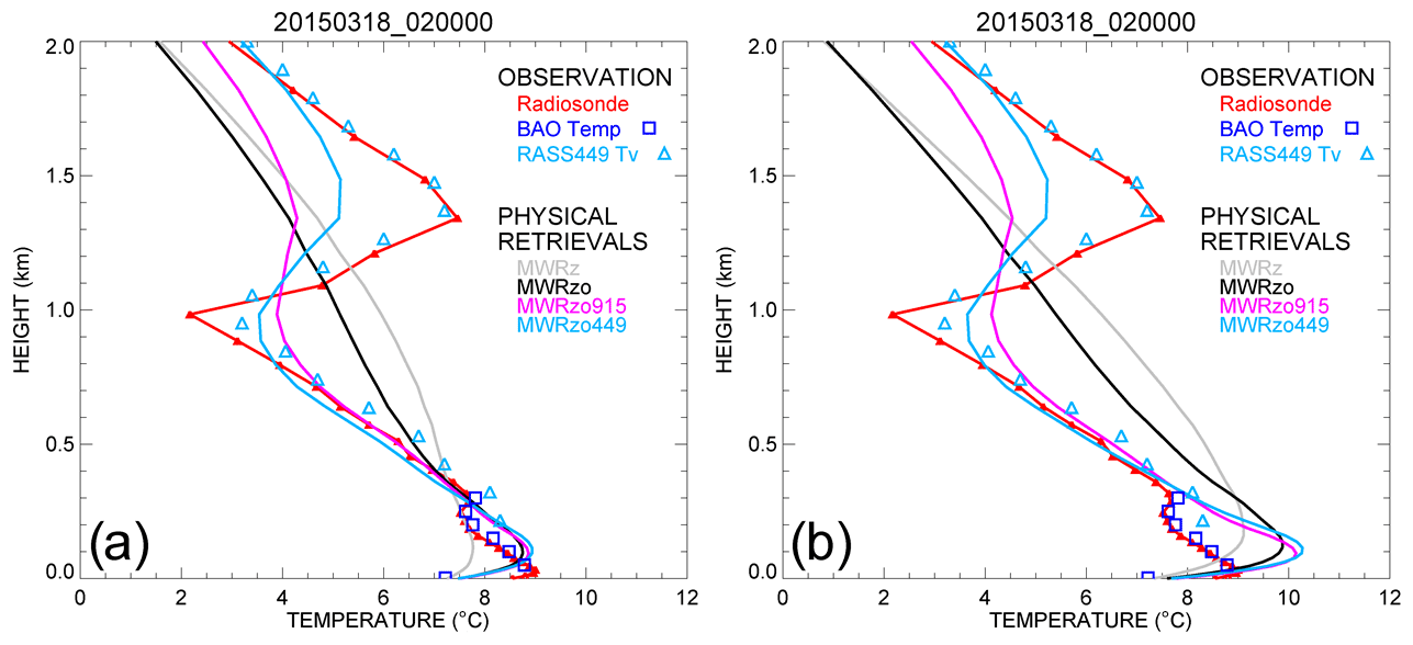
Figure 5 As in Fig. 2 but for 18 March 2015 at 02:00 UTC. The RASS 449 virtual temperature is included as light blue triangles. Panels (a) shows the PRs obtained after applying the radiosonde BC, and (b) shows the PRs obtained after applying the TROPoe BC on the MWR T_bs.

Figure 5 also illustrates the difference in the temperature profiles, especially between 0–300 m a.g.l., for the two different bias-correction schemes, which show noticeable differences in the biases of the opaque channels (especially important for the near-ground retrievals) presented in Fig. 1. As expected, the radiosonde BC method yielded a retrieved profile closer to the radiosonde temperature profile than when using TROPoe BC, for which the inversion in the temperature profile close to the surface is too accentuated (particularly the black, magenta, and cyan lines, all of which used oblique scan data).

The relative statistical behavior (Pearson correlation, RMSE, and bias) of the PRs for both temperature and mixing ratio against radiosondes is shown in Fig. 6, using both bias-correction approaches. PRs obtained after applying the radiosonde BC (Fig. 6a) present overall smaller RMSE and bias (the latter almost equal to zero up to 3 km a.g.l.) and slightly higher correlations compared to the statistics of the PRs obtained after applying the TROPoe BC (Fig. 6b). This could be expected since for the comparison in Fig. 6a a subset of the radiosondes was already used for the T_b bias correction. Also, the different retrievals show a narrower distribution for the panels in Fig. 6a. Nevertheless, the results obtained when applying either bias-correction methods (in Fig. 6a, b) consistently show the improvement obtained when the RASS observations are used, with relatively smaller bias and RMSE in the 3 km layer a.g.l. The correlation is mainly improved above 1 km, when RASS observations are included.

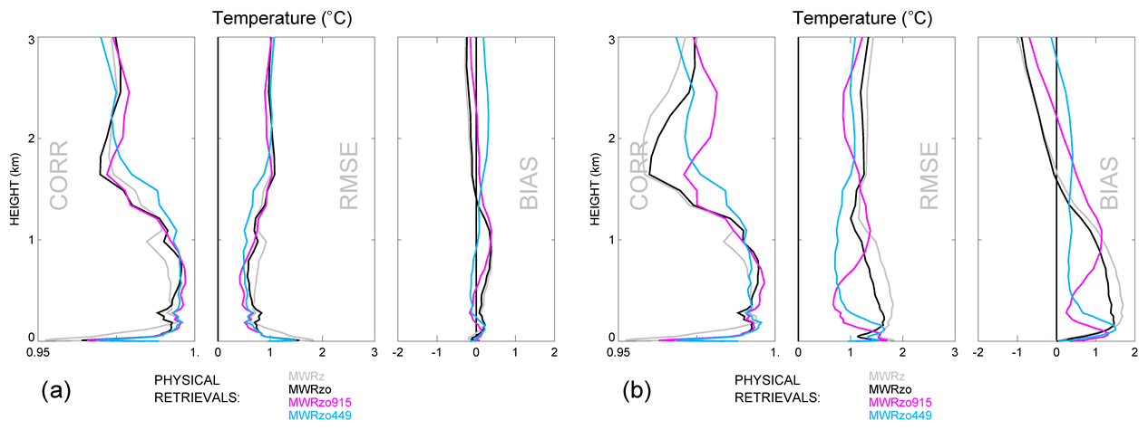
Figure 6 Pearson correlation, RMSE, and mean bias for temperature profiles of MWRz in gray, MWRzo in black, MWRzo915 in magenta, and MWRzo449 in light blue for the radiosonde BC bias-correction method in (a) and TROPoe BC method in (b).

Besides temperature profiles, the PRs also provide water vapor mixing ratio profiles. It is understandable that the different configurations of PRs are not noticeably different from each other in relation to moisture, because the T_v observations from the RASS are dominated by the ambient temperature (not moisture), and thus have little impact on the water vapor retrievals. We found that the AQKernel values are almost identical for all four PR configurations (not shown). Detailed statistical evaluation of the PR mixing ratio profiles is presented in Fig. 7, also averaged over all radiosonde events, and shows very similar correlations, RMSEs, and biases for all PRs, implying that the impact of including RASS observations in the retrieval is minimal on this variable. Finally, it is noted that Fig. 7 shows the mixing ratio of the data from TROPoe BC. The radiosonde BC mixing ratio results are almost identical.

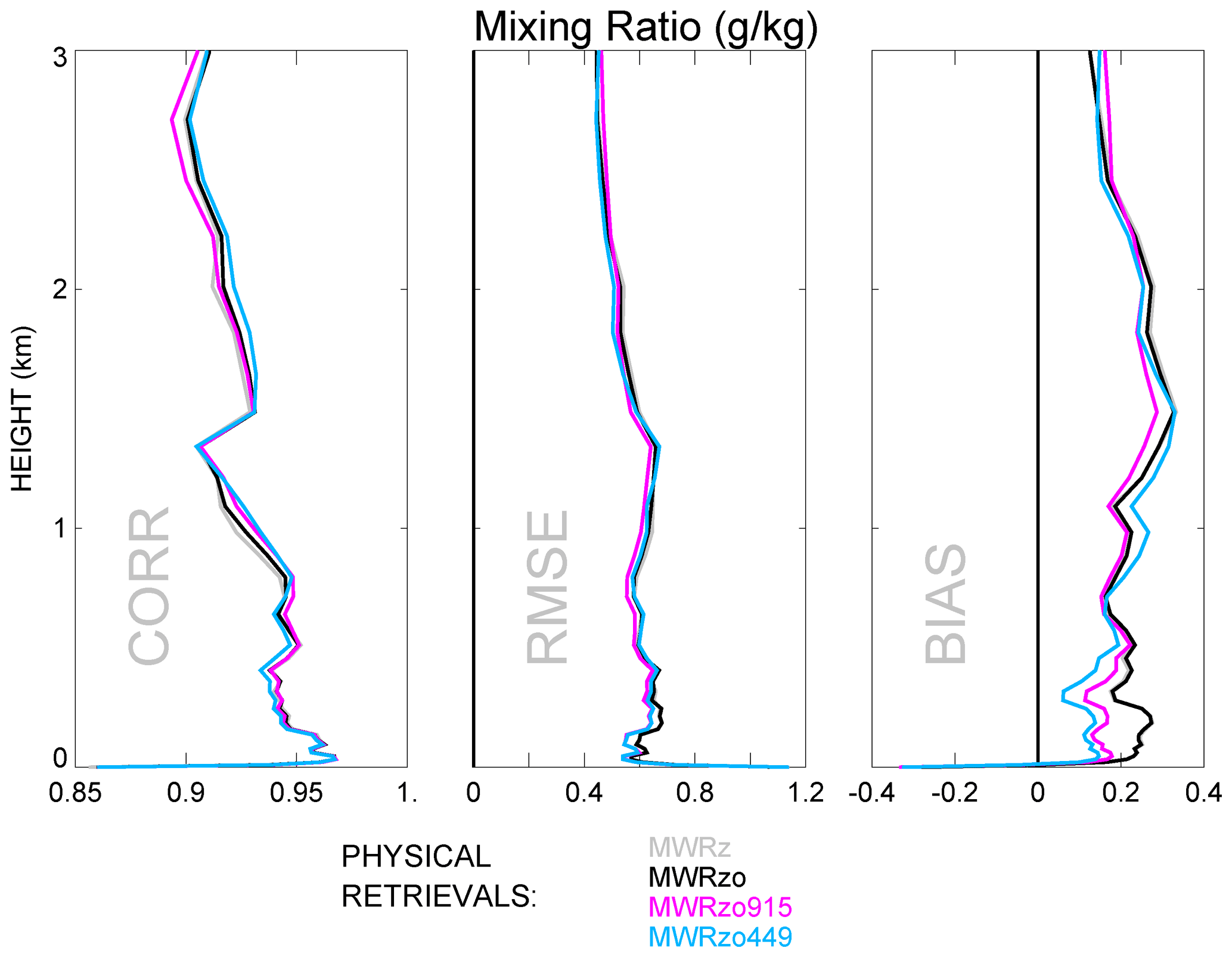
Figure 7 Same as the panels in Fig. 6b, but for mixing ratio, when using the TROPoe BC method on the MWR T_bs.

4.2 Statistics for the profiles least close to the climatology

Physical retrievals use climatological data as a constraint in the retrieval. Statistically, the averaged profiles of both temperature and moisture variables are very close to the climatological averages. However, the most interesting and difficult profiles to retrieve are the cases furthest from climatology (Löhnert and Maier, 2012). To check the behavior of the retrieved data in such “extreme” cases, the RMSE was first calculated for each radiosonde profile relative to the prior profiles for 37 vertical levels from the surface up to 3 km a.g.l., and then the 15 cases with the largest 0–3 km layer averaged RMSEs compared to the prior were selected.

Figure 8 shows the temperature statistical analysis for the entire radiosonde dataset (solid boxes) and for the 15 events far from the climatological mean (hatched boxes) for bias, RMSE, standard deviation of the differences between retrievals and radiosonde data, and Pearson correlation, calculated as the weighted averaged over the 37 vertical heights up to 3 km a.g.l.¹.

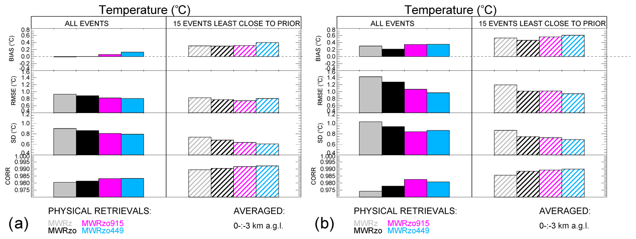
Figure 8 From top to bottom: biases (retrievals minus radiosonde), RMSEs, standard deviations of the difference between retrievals and radiosonde, and Pearson correlations for the four PR configurations, averaged from the surface to 3 km a.g.l., over all radiosonde data (solid boxes), and over the 15 extreme cases (hatched boxes). The data in panel (a) use radiosonde BC and in (b) TROPoe BC on the MWR T_bs.

Differences in the statistics when using the entire radiosonde dataset or the 15 extreme profiles are noticeable for all statistical estimators. The PRs that include RASS observations show better performance compared to the strictly MWR-only PR profiles (i.e., MWRz and MWRzo) for almost all statistical comparisons. This improvement is larger for the PRs using the TROPoe BC (Fig. 8b) compared to the PRs using the radiosonde BC (Fig. 8a). Three statistical estimators, RMSE, standard deviation, and Pearson correlation, show overall better values for the 15 extreme cases compared to the whole radiosonde dataset, for all PR configurations and both BC approaches. This is due to the fact that for this dataset the monthly averaged radiosonde profiles (for March and May particularly) depart quite substantially from the monthly prior profiles. For example, the averaged radiosonde profile in March is warmer by ∼7 ^∘C compared to the March prior (and in May by ∼5 ^∘C) in the first 3 km a.g.l.. Consequently, the extreme cases (mostly found in March) have the warmest radiosonde temperature profiles but are overall closer to the monthly averaged radiosonde profiles.

Table 2 includes the same data as in Fig. 8 but as a percentage of the improvement, compared to the MWRz retrievals.

Table 2 Retrieval improvements for different RASS/MWR configurations as a percentage compared to MWRz.

The results presented in Table 2 show improvements in all statistical estimations when including RASS observations, with improvements in RMSE between 10 % and 20 %, demonstrating the positive impact derived by the inclusion of the active measurements, regardless of the bias-correction method used, but larger for the TROPoe BC data because there is more room for improvement when this BC method is used. Improvements in the Pearson correlation coefficients are small because correlation, determined during XPIA by the overall temperature structure with height and diurnal cycle, is already good, leaving little room for improvement.

4.3 Virtual temperature profile statistics

Using the physical retrieval outputs, “retrieved virtual temperature profiles” can also be calculated. In this section the direct comparison of these retrieved virtual temperature profiles and RASS virtual temperature profiles to the original radiosonde is shown. With this comparison we want to show how the biases of the retrieved profiles relate to the original RASS T_v biases.

Figure 9 shows T_v retrieved profile biases compared to the original radiosonde data. These T_v profiles and RASS 915 and RASS 449 T_v bias data are interpolated onto a regular vertical grid, going from 200 m to 1.6 km with a 100 m resolution, for easy comparison.

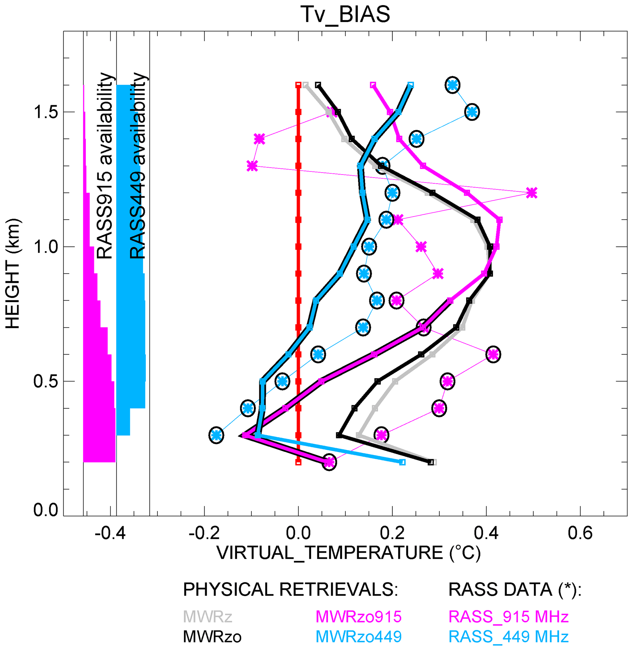
Figure 9 Bias of virtual temperature for all PR configurations compared to the original radiosonde measurements. A zero bias is denoted by the red line. RASS data biases are marked by asterisks and by additional circles for the RASS data with more than 50 % availability, according to the availability bar charts on the left. All PR profiles are derived after applying the radiosonde BC method.

While RASS 449 data are available at almost all heights up to 1.6 km, the RASS 915 data availability decreases considerably with height, decreasing to 50 % availability around 800 m a.g.l.. The PRs that include RASS data, MWRzo915 and MWRzo449 are also marked with additional black lines at the heights with at least 50 % of relative RASS data availability. In agreement with Fig. 6a, this figure clearly shows the superiority of the MWRzo449 and MWRzo915 (in the layer with >50 % RASS data availability) compared to the MWRz and MWRzo configurations, which do not include RASS data. For MWRzo449, RASS 449 data were almost always available; therefore it is easy to identify a similarity between the T_v bias profiles of the RASS 449 and the PRs including it. Thus, for the MWRzo449 the T_v bias is more uniform through the heights compared to all other PRs that do not include RASS data. Moreover, it is noted that a roughly constant offset between the MWRzo449 T_v and RASS 449 T_v biases profiles, with their averaged difference equal to ∼0.08 ^∘C (when the radiosonde BC is used), and to ∼0.32 ^∘C (when the TROPoe BC is used, not shown), over the ∼1.3 km (0.3–1.6 km) atmospheric layer where more than 50 % of the RASS 449 measurements are available, uniformly distributed through the heights. The inclusion of the RASS into the PRs does reduce the values of the biases in the retrievals even below the values of the RASS biases, because of the combined information from RASS and MWR.

5 Conclusions

In this study, data collected during the XPIA field campaign were used to test different configurations of a physical iterative retrieval (PR) approach in the determination of temperature and humidity profiles from data collected by microwave radiometers, surface sensors, and RASS measurements. The accuracy of several PR configurations was tested: two configurations made use only of surface observations and MWR observed brightness temperature (zenith only, MWRz; zenith plus oblique, MWRzo), while two others included the active virtual temperature profile observations available from co-located RASS (one, RASS 915, associated with a 915 MHz and the other, RASS 449, associated with a 449 MHz wind profiling radar). Radiosonde launches were used for verification of the retrieved profiles. In Appendix A, the performance of MWRz and MWRzo retrieved profiles and neural network retrieved profiles against the radiosondes was evaluated.

To remove any observational systematic error in the MWR T_b observations, two bias-correction procedures were tested. The first one takes advantage of the many radiosondes launched during XPIA, and the second one uses profiles. As expected, the radiosonde bias-correction method gives retrieved profiles closer to the radiosonde temperature profiles than when using the climatologically based method. Nevertheless, our results show that regardless of the bias-correction method used, the inclusion of the observations from the active RASS instruments in the PR approach improves the accuracy of the temperature profiles by around 10 %–20 % compared to the PR configuration using only surface observations and MWR observed brightness temperature from the zenith scan. Of the PR configurations tested, generally better statistical agreement is found with the radiosonde observations when the RASS 449 is used together with the surface observations and brightness temperature from the zenith and averaged oblique MWR observations.

The Akernel and the posterior covariance matrices for temperature are used to derive the one-sigma uncertainty, vertical resolution, and cumulative degree of freedom as a function of height for the different PRs and the level-to-level correlated uncertainty of the retrievals. Results show that the inclusion of the active instruments improves all of the above-mentioned variables in the 0–3 km layer, including at heights between 2–3 km that are above the maximum RASS height. Thus, the positive impact of the RASS observations extends into the atmosphere above the height of measurements themselves.

Furthermore, 15 cases when temperature profiles from the radiosonde observations were the furthest away from the mean climatological average were selected, and the statistical comparison was reproduced over this subset of cases. These are the cases usually the most difficult to retrieve and the most important to forecast; therefore, it is essential to improve the retrievals in these situations. Even for this subset of selected cases the inclusion of active sensor observations in the PRs is found to be beneficial.

Finally, the impact of the inclusion of RASS measurements on the retrieved humidity profiles was considered, but the inclusion of RASS observations did not produce significantly better results, compared to the configurations that do not include them. This was not a surprise as RASS measures virtual temperature, effectively adding very little extra information to the water vapor retrieval. In this case a better option would be to consider adding other active remote sensors such as water vapor differential absorption lidars (DIALs) to the PRs. Turner and Löhnert (2021) showed that including the partial profile of water vapor observed by the DIAL substantially increases the information content in the combined water vapor retrievals. Consequently, to improve both temperature and humidity retrievals a synergy between MWR, RASS, and DIAL systems would likely be necessary.

Appendix A

The neural network (NN) retrievals developed by the vendor explicitly for XPIA use a training dataset based on a 5-year climatology of profiles from radiosondes launched at the Denver International Airport, ∼56 km southeast from the XPIA site. NN-based MWR vertical retrieval profiles were obtained using the zenith or an average of two oblique elevation scans, 15 and 165^∘ (not including the zenith), all with 58 levels extending from the surface up to 10 km, with a nominal vertical grid depending on the height (every 50 m from the surface to 500 m, every 100 m from 500 m to 2 km, and every 250 m from 2 to 10 km, a.g.l.).

Figure A1 shows composite NN vertical profiles of temperature (separately for the zenith and averaged obliques) calculated for radiosonde launch times and the corresponding PR profiles already introduced in Fig. 6a, b with additional TROPoe retrievals without any bias correction. For a proper comparison, only MWRz and MWRzo profiles are used, without including RASS measurements. It has to be noted that since the “NN oblique” retrieval provided by the manufacturer of the radiometer does not include the zenith, this configuration cannot be considered exactly equivalent to the MWRzo PR.

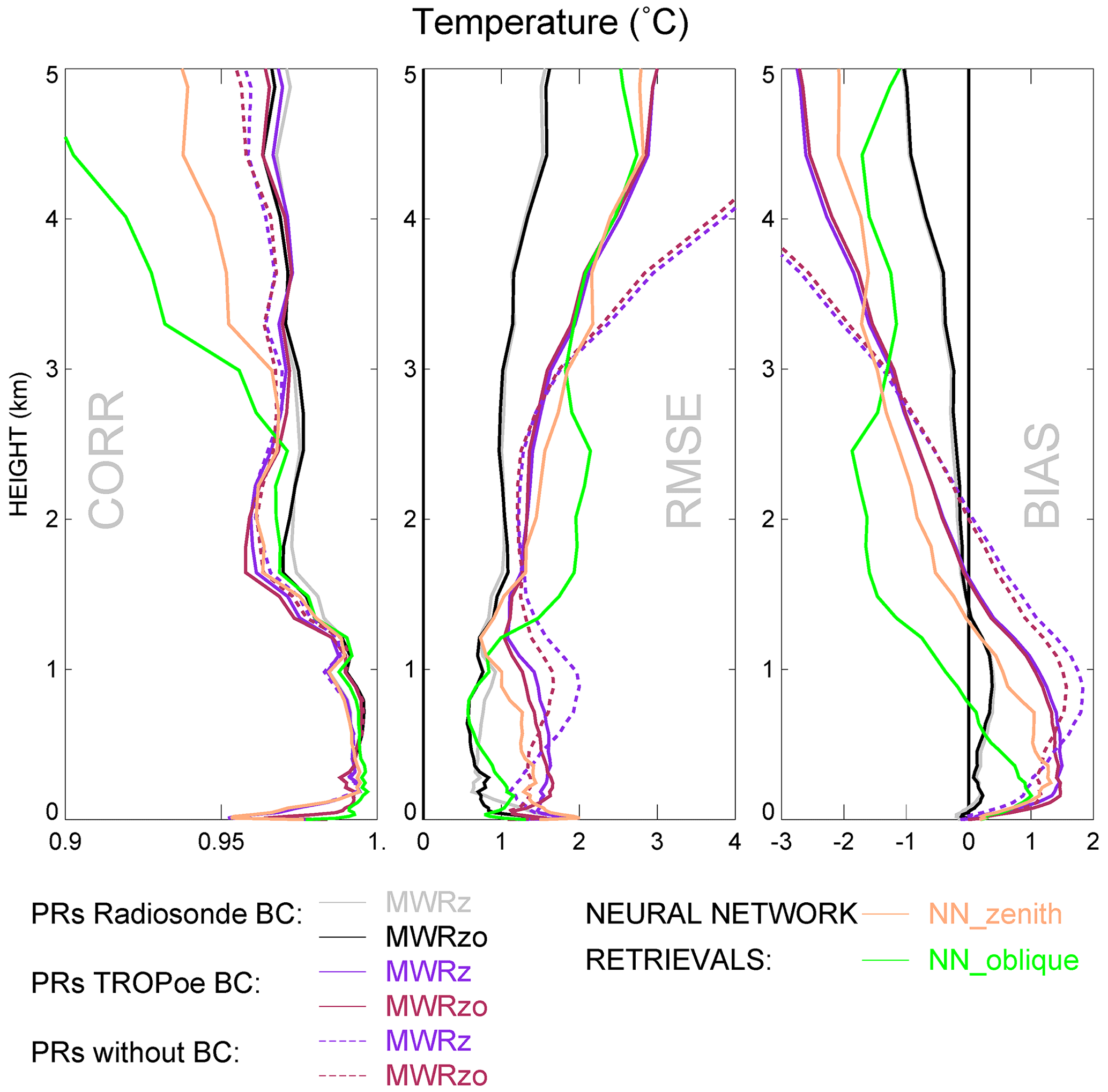
Figure A1 Pearson correlation, RMSE, and mean bias for temperature profiles for MWRz in gray (and purple) and MWRzo in black (and maroon) when the radiosonde BC (and the TROPoe BC) method is applied. TROPoe temperature retrievals without any bias correction are shown for MWRz in dashed purple and for MWRzo in dashed maroon. Included in this figure are the NN temperature profiles, from the zenith scan (in beige) and from the averaged oblique scans (in green).

Another difference to point out is that, while the MWR T_b data have been bias-corrected before being used in the PR configurations, as discussed in Sect. 3.2, the NN retrievals use the uncorrected T_b, since it was non-trivial to reprocess those retrievals. For additional comparison we included TROPoe retrievals that use uncorrected T_bs. Martinet et al. (2015) showed that when it is possible to bias-correct the MWR T_b before applying the NN retrieval technique, the NN retrievals are not impacted below 1 km a.g.l., but a clear improvement of NN retrievals in terms of RMSE and bias is observed between 1 and 3 km altitude. As is visible in Fig. A1, this is the layer of the atmosphere where the NN profiles (beige and green lines) have larger bias and RMSE, compared to the PR profiles.

When the radiosonde BC method is used, the MWRz and MWRzo PRs (gray and black lines) present better statistics through the entire profiles shown in Fig. A1, with larger values of the correlation coefficient and smaller values of RMSE and bias. The oblique-only NN profiles (in green) show comparable statistics to the PRs employing the radiosonde BC method up to 1 km a.g.l., with degraded performances above this height. Above 1 km a.g.l., the zenith NN profiles (in beige) do better than the oblique NN in terms of RMSE and bias. When the TROPoe BC method is used, the MWRz and MWRzo PRs (purple and maroon lines) perform better than the NN profiles only in terms of RMSE and bias, and only between 1.5 and 3 km a.g.l. The PRs without any T_b bias correction (dashed lines in Fig. A1) clearly indicate that the BC is useful and needed, showing very noticeable degradation in all three statistical measures above 3 km and larger RMSE and bias in 0.5–1.5 km a.g.l. compared to the TROPoe BC method.

The better performance obtained by the MWRz and MWRzo PRs that use the radiosonde BC approach demonstrates the importance of having an accurate and reliable method for bias-correcting the MWR.