Algorithm theoretical basis for ozone and sulfur dioxide retrievals from DSCOVR EPIC

On board the Deep Space Climate Observatory (DSCOVR), the first Earth-observing satellite at the L1 point (the first Lagrangian point in the Earth–Sun system), the Earth Polychromatic Imaging Camera (EPIC) continuously observes the entire sunlit face of the Earth. EPIC measures the solar backscattered and reflected radiances in 10 discrete spectral channels, four of which are in the ultraviolet (UV) range. These UV bands are selected primarily for total ozone (O₃) and aerosol retrievals based on heritage algorithms developed for the series of Total Ozone Mapping Spectrometers (TOMS). These UV measurements also provide sensitive detection of sulfur dioxide (SO₂) and volcanic ash, both of which may be episodically injected into the atmosphere during explosive volcanic eruptions. This paper presents the theoretical basis and mathematical procedures for the direct vertical column fitting (DVCF) algorithm used for retrieving total vertical columns of O₃ and SO₂ from DSCOVR EPIC. This paper describes algorithm advances, including an improved O₃ profile representation that enables profile adjustments from multiple spectral measurements and the spatial optimal estimation (SOE) scheme that reduces O₃ artifacts resulting from EPIC's band-to-band misregistrations. Furthermore, this paper discusses detailed error analyses and presents intercomparisons with correlative data to validate O₃ and SO₂ retrievals from EPIC.

1 Introduction

The Deep Space Climate Observatory (DSCOVR) was launched on 11 February 2015 and after a 116 d journey successfully maneuvered into its Lissajous orbit around the first Earth–Sun system Lagrangian (L1) point, which is about 1.5×10⁶ km from the Earth and located between the Sun and the Earth on the ecliptic plane. At the L1 point, where the net gravitational forces equal the centrifugal force, DSCOVR orbits the Sun at the same rate as the Earth, staying closely in line along the Sun and the Earth, thus allowing the Earth-pointing EPIC to continuously monitor the entire sunlit planet.

The Earth Polychromatic Imaging Camera (EPIC) measures the solar backscattered and reflected radiances from the Earth using a two-dimensional (2048×2048) charged-coupled device (CCD) recording a set of 10 spectral images successively using different narrowband filters. While EPIC may continuously observe the Earth from the vicinity of the L1 point, only a number of spectral image sets are taken in a day, limited by accessible contact windows of the two ground stations located in Wallops island (Virginia) and Fairbanks (Alaska). Currently, between 13 and 22 spectral image sets, recorded at a sampling rate of one set in every 110 min during boreal winter and every 65 min during boreal summer, are transmitted back to the ground stations in a day.

EPIC takes about 6.5 min to complete an image set. The first in the set is the blue band (centered at 443 nm), which takes ∼2 min to complete the imaging at native resolution (2048×2048 pixels). The images of the nine remaining bands are sequentially recorded at a reduced resolution (1024×1024 pixels, achieved through an onboard average of 2×2 pixels), separated by a time cadence of ∼30 s between adjacent bands. Due to the Earth's rotation and spacecraft jitter, each spectral image records a slightly different (i.e., rotated) sunlit hemisphere. As a result, the images of two different channels appear to be displaced from each other, usually by a distance of about one to a few native pixels, depending on their observation time difference.

Each native pixel has a ∼1 arcsec or $\mathrm{2.778}\times {\mathrm{10}}^{-\mathrm{4}}{}^{\circ }$ angular instantaneous field of view (IFOV), yielding a geometric ground footprint size of $\sim \mathrm{8}\times \mathrm{8}$ km² at the image center of the sunlit disk. The effective footprint size is about 10×10 km², which is larger than the geometric one due to the effect of the optical point-spread function of the EPIC imaging system. For a reduced-resolution image (1024×1024 pixels), the effective central ground IFOV size is about 18×18 km², which is significantly smaller than the nadir footprints of some past and present satellite instruments that provided global ozone mapping from the low Earth orbit (LEO), such as the Total Ozone Mapping Spectrometer (TOMS; nadir pixel size 50×50 km²) on a series of satellites, the Scanning Imaging Absorption Spectrometer for Atmospheric Cartography (SCIAMACHY; 60×30 km²; Bovensmann et al., 1999) on ESA's ENVIronmental SATellite (ENVISAT), the Ozone Mapping and Profiler Suite Nadir Mapper (OMPS-NM; 50×50 km²; Flynn et al., 2014) on the Suomi National Polar Partnership (SNPP), and the Global Ozone Monitoring Experiment-2 (GOME-2; Callies et al., 2000; Munro et al., 2016) on Metop-A (40×40 km²), Metop-B (80×40 km²), and Metop-C (80×40 km²). Though it is slightly larger than the nadir footprint of the Ozone Monitoring Instrument (OMI; 13×24 km²; Levelt et al., 2006) on Aura and the OMPS-NM (17×13 km²; Flynn et al., 2016) on NOAA-20, as well as much bigger than that of the TROPOspheric Monitoring Instrument (TROPOMI; 5.5×3.5 km²; Veefkind et al., 2012) on the ESA Sentinel-5 Precursor (S5P), EPIC's spatial resolution is sufficiently high to map small-scale O₃ natural variations and observe many volcanic emissions, from degassing to eruption.

EPIC, combining moderate spatial resolution with high temporal cadences from the unique vantage point of L1, provides unprecedented Earth observations from sunrise to sunset simultaneously (see Fig. 1). This synoptic (i.e., concurrent, globally unified, and spatially resolved) perspective is quite distinctive from satellite observations from an LEO or geostationary Earth orbit (GEO): LEO observations are often made within a narrow range of local time with a small number of samplings at a location per day, while GEO observations have limited spatial coverage, constrained to roughly 60^∘ away from its position. The EPIC observations can have simultaneous co-located observations with measurements from any contemporaneous LEO and GEO platforms, allowing direct comparisons and synergistic use of data acquired from different perspectives. This overlapping feature has been exploited to calibrate some EPIC channels by matching its measured albedo values to those of OMPS-NM on SNPP (Herman et al., 2018).

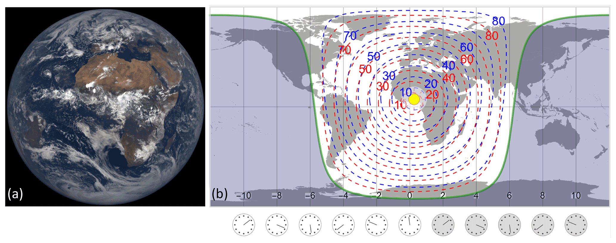
Figure 1 (a) Example of the EPIC field of view (FOV): EPIC Earth image at 11:40:31 UTC on 4 September 2015. Image source: NASA EPIC Team, accessed via https://epic.gsfc.nasa.gov (last access: 1 October 2022). (b) Viewing and illumination angles are taken from FOV on the left. The subsolar point is marked on the map with a yellow dot. The area shaded with midnight blue is in the dark, i.e., without direct sunlight, while the unshaded area is the sunlit hemisphere, with sunrise on the left (west of subsolar point) and sunset on the right (east of subsolar point). Contours of solar zenith angles (SZAs, blue dashed lines) and viewing zenith angles (VZAs, red dashed lines), going from 10 to 80^∘ with a step of 10^∘, are shown in the sunlit area. Note that the SZA (θ_s) and VZA (θ_v) of an EPIC IFOV have similar values, and both angles increase as the IFOV moves from the center towards the edge of the sunlit disk.

The 10 narrow bands of EPIC, spanning ultraviolet (UV), visible, and near-infrared wavelengths, are selected to yield diverse information about the Earth, from atmospheric compositions to surface reflectivity and vegetation. Four of the 10 bands measure UV spectral radiances, which are primarily used for total ozone (O₃) retrievals. These UV bands also provide sensitive detection of sulfur dioxide (SO₂) and volcanic ash, both of which may be episodically injected into the atmosphere during explosive volcanic eruptions.

This paper describes algorithm physics, model assumptions, mathematical procedures, and error analyses for the direct vertical fitting (DVCF) algorithm. We show examples to illustrate the high accuracy of O₃ and SO₂ retrievals achieved by applying the DVCF algorithm to spectral UV radiance measurements of DSCOVR EPIC. Lastly, we validate the DSCOVR EPIC O₃ and SO₂ through intercomparisons with correlative data.

2 Algorithm physics

Algorithm physics is a term first used by Chance (2006) to denote the physical processes contributing to the spaceborne measurement of radiance spectra. A measured radiance L_m (in units of $\mathrm{W}\cdot {\mathrm{sr}}^{-\mathrm{1}}\cdot {\mathrm{m}}^{-\mathrm{2}}\cdot {\mathrm{nm}}^{-\mathrm{1}}$) from space consists of sunlight photons within a narrow spectral range (typically <2 nm), specified by the instrument spectral response function S (ISRF, e.g., EPIC UV filter transmissions shown in Fig. 2), and is modeled as

$$\begin{array}{}\text{(1)}& L_{\mathrm{M}}={\displaystyle \frac{\int S\left(\mathit{\lambda }\right)I_{\mathrm{TOA}}\left(\mathit{\lambda }\right)F\left(\mathit{\lambda }\right)\mathrm{d}\mathit{\lambda }}{\int S\left(\mathit{\lambda }\right)\mathrm{d}\mathit{\lambda }}},\end{array}$$

where F(λ) (in units of $\mathrm{W}\cdot {\mathrm{m}}^{-\mathrm{2}}\cdot {\mathrm{nm}}^{-\mathrm{1}}$) is the monochromatic spectral solar irradiance, and I_TOA(λ) is the Sun-normalized monochromatic top-of-the-atmosphere (TOA) radiance (in units of sr⁻¹) for a wavelength λ (in units of nm). The Sun-normalized measured radiance I_M for a spectral band is defined as $I_{\mathrm{M}}=L_{\mathrm{M}}/F_{\mathrm{M}}$, where $F_{\mathrm{M}}=\int S\left(\mathit{\lambda }\right)F\left(\mathit{\lambda }\right)\mathrm{d}\mathit{\lambda }/\int S\left(\mathit{\lambda }\right)\mathrm{d}\mathit{\lambda }$, and the λ integrations in these equations are performed over the valid range of the ISRF S for the spectral band. Hereafter we drop “Sun-normalized” when referring to I_M, which is simply called measured radiance. Quantities for a spectral band are flux-weighted bandpass averages to account for the differential contributions from individual wavelengths within the bandpass. Without loss of generality, I_TOA(λ) and other spectral-dependent quantities are hereafter used to denote flux-weighted bandpass averages, with λ representing the characterized wavelength of the spectral band.

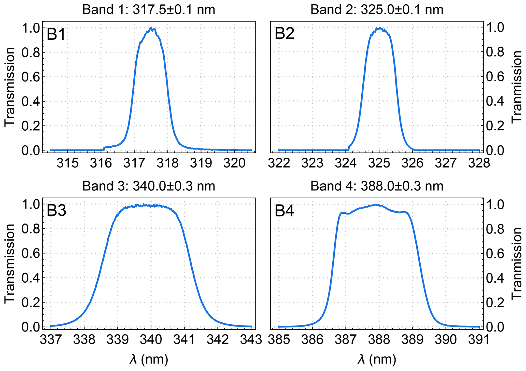
Figure 2 Filter transmission functions for the four EPIC UV channels. The widths are ∼1 nm for EPIC bands 1 and 2, similar to those for TOMS and OMPS-NM. Note that the filter transmissions as functions of wavelength are measured in the air (see Fig. 1 in Herman et al., 2018). Here we have converted the wavelength in the air to wavelength in a vacuum using the formula of Edlén (1966). The filter values are normalized to 1 at band centers (noted on top of each panel with uncertainty).

To reach a sensor at TOA, sunlight photons are either back-scattered by air molecules or particles or reflected by the underlying Earth surface. As these photons traverse through the atmosphere along many possible optical paths connecting the Sun to the sensor, they may be absorbed by the underlying surface or by some atmospheric constituents, such as trace gases (e.g., O₃ and SO₂) and light-absorbing particles (e.g., dust and smoke). The photons that complete the journey carry information about atmospheric absorbers along their paths. The accumulation of photons from each contributing path yields the TOA radiance, which may be modeled with radiative transfer (RT) simulation if the properties of surface reflection as well as atmospheric absorption and scattering are known explicitly. The ability to model the TOA radiance accurately is the prerequisite for interpreting the observations and relating the gas absorptions with TOA radiance measurements.

We next describe the characteristics of UV photon sampling of the atmosphere and the construction of surface and atmospheric models to enable proper simulation of the photon sampling of the atmosphere. Dividing the atmosphere into infinitesimal thin layers, the quantity that specifies the photon sampling is the mean path length of photons traversing through a layer. This mean path length normalized by the geometric thickness of the layer is the local or altitude-resolved air mass factor (AMF, m_z). The proper simulation of photon sampling requires the modeled mean path length through each layer to closely match that in the actual observing condition.

In theory, a TOA radiance, I_TOA, depends on the viewing illumination geometry, the optical properties of the atmospheric constituents (both absorbers and non-absorbers), and their amounts and vertical distributions, as well as on the reflective properties of the underlying surface. For a wavelength λ, I_TOA can be expressed as the sum of two contributions,

$$\begin{array}{}\text{(2)}& I_{\mathrm{TOA}}=I_{\mathrm{a}}+I_{\mathrm{s}},\end{array}$$

where I_a consists of solar photons scattered once or more by molecules and particles in the atmosphere without interacting with the underlying surface, and I_s represents solar photons reflected at least once or multiple times by the underlying surface.

2.1 Path radiance

I_a is also known as the atmospheric path radiance, i.e., photons backscattered to the sensor along a path without any intersection with the underlying surface. Conceptually it is the accumulation of TOA photons that are last backscattered toward the sensor along the line of sight from atmospheric layers at different levels of extinction optical depths. Algebraically it is expressed as the path integration of virtual emission J(t) (Dave, 1964) in the direction specified by the view zenith angle (θ_v), attenuated ($e^{-t/\mathit{\mu }}$, where μ=cos θ_v) by atmospheric scattering and absorption, over the extinction optical depth t along the path of line of sight from the top (t=0) to the bottom (t=τ) of the atmosphere:

$$\begin{array}{}\text{(3)}& I_{\mathrm{a}}=\underset{\mathrm{0}}{\overset{\mathit{\tau }}{\int }}J\left(t\right)e^{-t/\mathit{\mu }}\mathit{\omega }\left(t\right)\mathrm{d}t/\mathit{\mu }.\end{array}$$

The source of virtual emission, J(t), consists of all the photons scattered towards to the sensor, including photons of the direct solar radiation being scattered once only and photons of diffuse radiation (i.e., photons scattered to level t) being scattered once more at t. The strength of the virtual emission of a thin layer at t is proportional to its scattering optical thickness, which is equal to the product of the layer total optical thickness (dt) and the single-scattering albedo ω(t) (defined as the ratio of layer scattering optical thickness over the layer total optical thickness). Here we use $\mathrm{\Psi }\left(t\right)=J\left(t\right)e^{-t/\mathit{\mu }}\mathit{\omega }\left(t\right)/\mathit{\mu }$ to represent the radiance contribution per unit optical thickness to I_a from a layer at t. Equation (3) describes how the solar photons sample the atmosphere from top to bottom and how atmospheric absorption is directly imprinted (via the attenuation $e^{-t/\mathit{\mu }}$) on the path radiance.

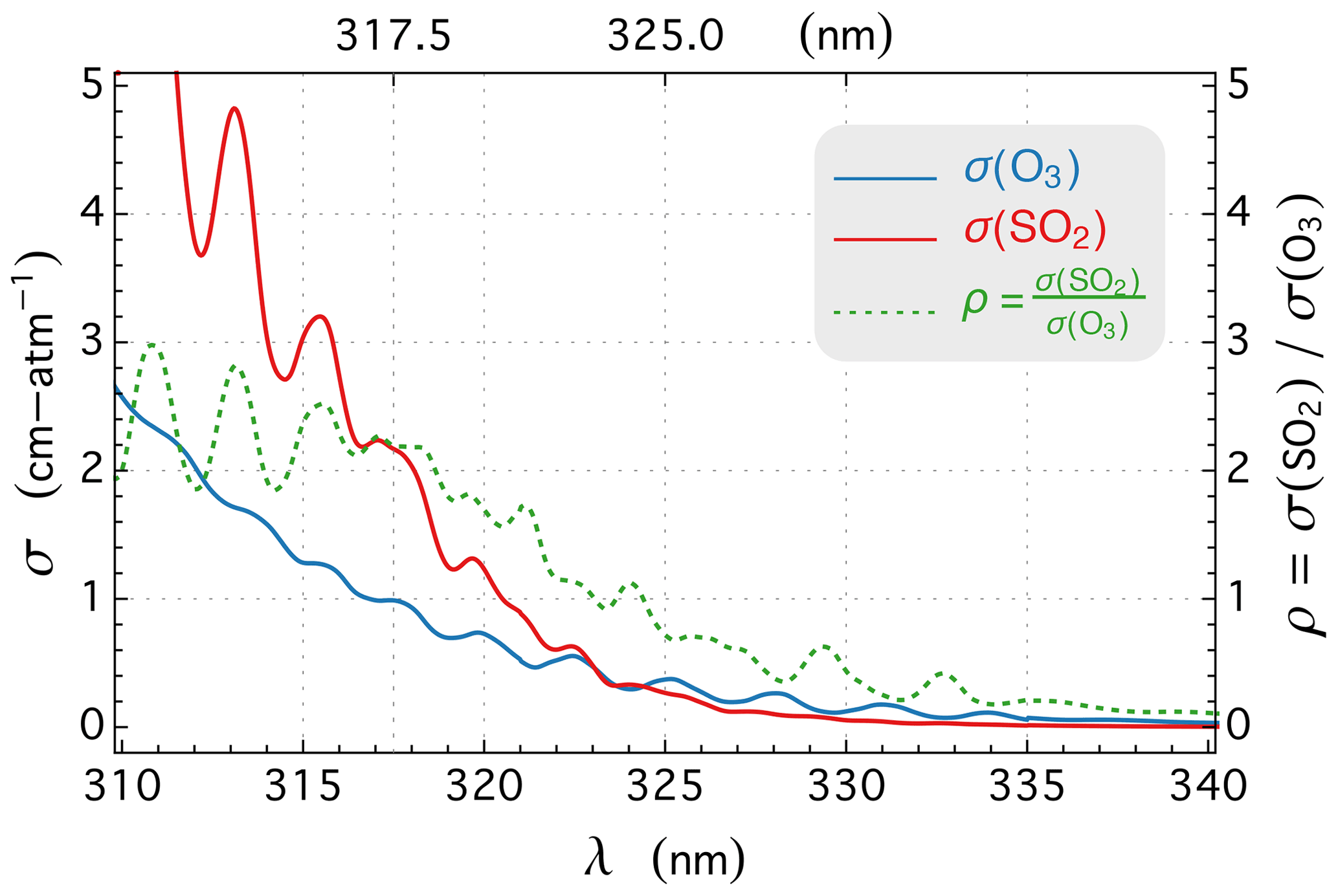
A path radiance I_a for a molecular (i.e., an aerosol- and cloud-free) atmosphere with absorption from trace gases can be accurately determined with RT simulations. For example, the path radiances for the low and high zenith angle geometries (see Fig. 3b) are calculated with a vector RT code (e.g., TOMRAD, Dave, 1964, or VLIDORT, Spurr, 2006) as a function of wavelength for a molecular atmosphere with the O₃ profile X₁ in Fig. 3a, and the corresponding radiance contributions to the path radiances at EPIC bands 1 and 2 are shown in Fig. 3c. The radiance contribution function (RCF) for a wavelength in the UV range (300–400 nm) is determined by Rayleigh scattering and absorption by trace gases (primarily O₃). O₃ is ubiquitous in the atmosphere, with the bulk of it located in the stratosphere (e.g., Figs. 3a or 11), and its absorption cross-sections σ(O₃) increase rapidly with shorter wavelengths in the UV range (see Fig. 13). Rayleigh scattering, whose cross-sections are proportional to $\frac{\mathrm{1}}{{\mathit{\lambda }}^{\mathrm{4}}}$, also increases with shorter wavelength. The strong O₃ absorption and large Rayleigh cross-sections at short wavelengths greatly reduce the number of solar photons reaching the lower atmosphere. Conversely, at longer wavelengths, weaker O₃ absorption and smaller Rayleigh cross-sections allow more solar photons to reach the lower atmosphere where higher air density increases the intensity of backscattering. Similar to the effect of reducing wavelength, lengthening the slant path (by increasing solar, viewing, or both zenith angles) would enhance ozone absorption and Rayleigh scattering along the slant path, raising the altitude profile of RCF. These spectral and angular characteristics of RCF are illustrated in Fig. 3c, which shows the normalized RCFs ($\mathit{\psi }=\mathrm{\Psi }/I_{\mathrm{a}}$) of EPIC bands 1 and 2 for two different observation geometries and a midlatitude O₃ profile labeled as X₁ in Fig. 3a. The results in Fig. 3c show that at longer wavelengths and lower zenith angles, path radiance contains more photons that are backscattered from the lower atmosphere. The RCF peak reaches ∼4 km altitude for band 2 at 5^∘ zenith angle, while at shorter wavelength and higher zenith angle, the RCF peak moves to the higher altitude, and it rises to ∼10 km for band 1 at 70^∘ zenith angle. The shifting shapes of RCF shown in Fig. 3c illustrate the changes in the photon sampling of the atmosphere with different wavelengths and zenith angles. The rising RCF peak position signifies diminishing sensitivity to absorptions below the peak while favoring those above it.

Figure 3 Sample results from RT simulations for a molecular atmosphere with O₃ profiles X₁ and X₂ in panel (a). Both X₁ and X₂ are midlatitude zone ($\mathrm{30}{}^{\circ }\le$ latitude $\le \mathrm{60}{}^{\circ }$) climatological O₃ profiles with the same total vertical column of 275 Dobson units, where 1 DU $=\mathrm{2.69}\times {\mathrm{10}}^{\mathrm{16}}$ molec. cm⁻². RT simulations are performed for two viewing illumination geometries: (1) low zenith angles of ${\mathit{\theta }}_{\mathrm{s}}={\mathit{\theta }}_{\mathrm{v}}=\mathrm{5}{}^{\circ }$ as well as a relative azimuthal angle of (RAA), $\mathit{\varphi }=\mathrm{45}{}^{\circ }$ and (2) high zenith angles of ${\mathit{\theta }}_{\mathrm{s}}={\mathit{\theta }}_{\mathrm{v}}=\mathrm{70}{}^{\circ }$ and $\mathit{\varphi }=\mathrm{45}{}^{\circ }$. (b) Path radiances I_a(X₁) for the low and high zenith geometries and their fractional changes ($\mathrm{\Delta }{I}_{\mathrm{a}}/I_{\mathrm{a}}$) when the O₃ profile is changed to X₂. (c) Normalized RCFs, ψ, for EPIC bands 1 and 2. Here ψ(t) is converted into ψ(lnP) by the multiplication of factor $\mathrm{d}t/\mathrm{dlnP}$. (d) Mean photon path lengths (m_a) of EPIC bands 1 and 2 as functions of altitude z for the low and high zenith geometries normalized by the respective geometric air mass factors, m_G.

The measurement sensitivity to a thin molecular absorber layer is equal to the product of the absorption cross-sections (σ) and the mean path length (m_a) of photons passing through the layer, where $m_{\mathrm{a}}=-\partial \ln I_{\mathrm{a}}/\partial {\mathit{\tau }}_z$ and τ_z is the absorption optical depth at the layer center altitude z. Note that the photon path length is equal to the geometric AMF, $m_{\mathrm{G}}=\mathrm{1}/\cos \left({\mathit{\theta }}_{\mathrm{s}}\right)+\mathrm{1}/\cos \left({\mathit{\theta }}_{\mathrm{v}}\right)$, for a plane-parallel atmosphere if there is no scattering. Figure 3d shows the mean optical path lengths of EPIC bands 1 and 2 as a function of altitude for the low and high zenith viewing illumination geometries, showing that m_a decreases rapidly as the layer descends nearing the surface due to fewer photons reaching the lower atmosphere, while m_a approaches m_G as the layer rises towards TOA due to fewer path-altering scatterings resulting from lower air density. In the upper troposphere and lower stratosphere (UTLS), m_a of the low zenith geometry usually exceeds m_G due to a significant fraction of photons undergoing multiple scattering below and within UTLS, while m_a of the high zenith geometry drops continuously from TOA down to the surface in the case when the RCF peak is sufficiently high that fewer multiple scatterings contribute to the path radiance. In general, the mean path length m_a is shorter for a wavelength with stronger O₃ absorption, which reduces the number of photons reaching the lower atmosphere. The variation of m_a with a changing altitude signifies the path radiance dependence on the absorber profile. The path radiance fractional change due to profile change ($\mathrm{\Delta }\mathbf{X}={\mathbf{X}}_{\mathrm{2}}-{\mathbf{X}}_{\mathrm{1}}$) can be expressed as

$$\begin{array}{}\text{(4)}& {\displaystyle \frac{\mathrm{\Delta }{I}_{\mathrm{a}}}{I_{\mathrm{a}}}}={\displaystyle \frac{I_{\mathrm{a}}\left({\mathbf{X}}_{\mathrm{2}}\right)-I_{\mathrm{a}}\left({\mathbf{X}}_{\mathrm{1}}\right)}{I_{\mathrm{a}}\left({\mathbf{X}}_{\mathrm{1}}\right)}}=-\underset{\mathrm{0}}{\overset{\mathrm{\infty }}{\int }}\mathrm{\Delta }X\left(z\right)\mathit{\sigma }\left(T_z\right)m_{\mathrm{a}}\mathrm{d}z,\end{array}$$

where T_z is the atmospheric temperature, and X₁(z) and X₂(z) are absorber concentration at altitude z. Figure 3b illustrates the change in path radiance caused by an O₃ profile change while keeping its total vertical column the same: lowering the O₃ profile (e.g., X₁ to X₂ in Fig. 3a) tends to increase the path radiance. Path radiance changes more with shorter wavelengths at higher zenith angles, thus becoming more sensitive to the shape of the O₃ profile. At low zenith angles, the change may have the opposite sign of the change at large zenith angle for certain wavelengths (e.g., the changes plotted as red solid lines for λ>316 nm in Fig. 3b), but the magnitude of change is much smaller, indicating that the path radiances under these conditions are primarily functions of total columns, since they are less sensitive to the profile shapes. The differential responses of the spectral path radiance to profile changes imply that more than one piece of information about O₃ may be contained in the multi-spectral measurements. Retrieval constrained by multi-spectral radiances instead of a single spectral band may achieve a more accurate O₃ measurement.

2.2 Surface reflection

The path radiance I_a includes backscattered photons that are independent of the underlying surface, while the surface contribution to TOA radiance, I_s (referred to as surface radiance hereafter), consists of photons reflected once or more from the surface. For a molecular atmosphere bounded by a surface with well-characterized optical reflection properties, the surface radiance I_s can be accurately predicted with RT modeling. For a Lambertian surface, which reflects radiation isotropically independent of the incident direction, the surface radiance I_s can be expressed as (Dave, 1964)

$$\begin{array}{}\text{(5)}& I_{\mathrm{s}}={\displaystyle \frac{T_{\downarrow }{r}_{\mathrm{s}}{T}_{\uparrow }}{\mathrm{1}-r_{\mathrm{s}}{S}_{\mathrm{b}}}},\end{array}$$

where r_s is the reflectance or albedo of the Lambertian surface, T_↓ is the total (direct and diffuse) transmittance from the Sun to the surface along the direction of incoming solar irradiation and T_↑ from the surface to the TOA along the viewing direction, and S_b is the atmospheric spherical albedo, which is the fraction of the reflected radiation backscattered from the overlaying atmosphere to the surface. The surface contribution from the Lambertian surface, I_s, may be described as the once-reflected radiance ($T_{\downarrow }{r}_{\mathrm{s}}{T}_{\uparrow }$), enhanced by the series of interactions: backscattering from the overlaying atmosphere and reflection from the underlying surface, which are accumulated to produce the amplification factor $\mathrm{1}/(\mathrm{1}-r_{\mathrm{s}}{S}_{\mathrm{b}})$.

The reflection property of a surface is represented by a bidirectional reflectance distribution function (BRDF), which specifies the angular distribution of reflected radiance as a fraction of directional incident spectral irradiance. Field measurements (Brennan and Bandeen, 1970) demonstrate that reflection from natural surfaces (such as cloud, water, and land surfaces) is anisotropic in the UV, exhibiting different apparent reflectances when viewed from different directions. For instance, a water surface looks bright when viewed from the direction near the specular reflection but is much darker outside the glitter (see, e.g., Fig. 4a). Here the apparent reflectance is the Lambertian equivalent reflectivity (LER), i.e., the isotropic reflectance r_s that reproduces the radiance I_s from a surface with an anisotropic BRDF at a viewing illumination geometry. This LER is also referred to as the geometry-dependent surface LER (GLER) to indicate its dependence on the viewing illumination geometry.

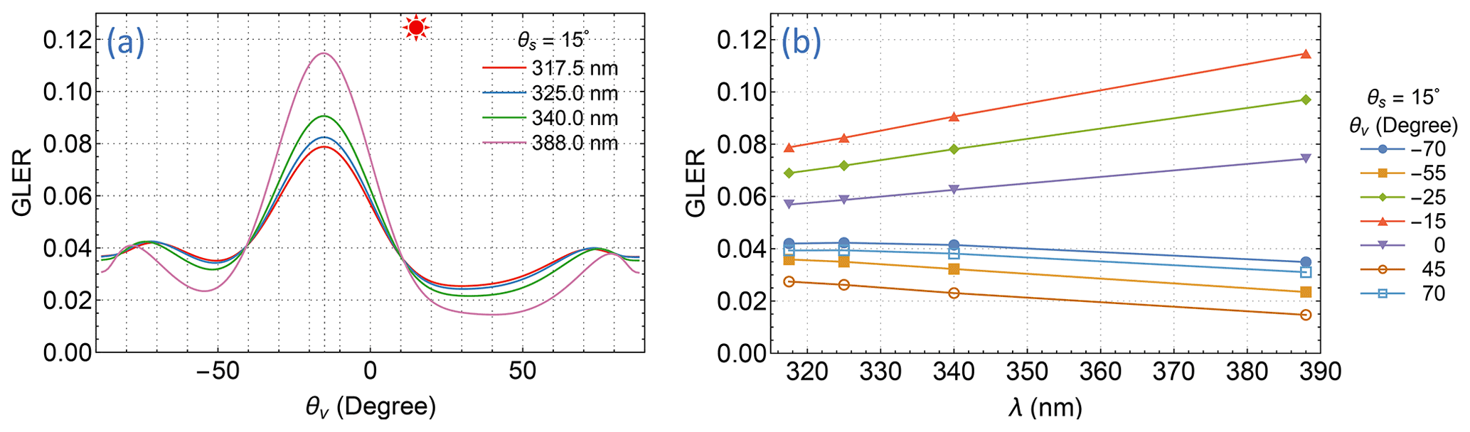
Figure 4 Apparent reflectances of an ocean surface described by a Cox–Munk BRDF (Cox and Munk, 1954a, b) for a wind speed of 6 m s⁻¹, viewed along the plane of incidence with the Sun at a zenith angle of ${\mathit{\theta }}_{\mathrm{s}}=\mathrm{15}{}^{\circ }$. (a) GLER at four EPIC UV bands vs. viewing zenith angle θ_v. Here positive θ_v denotes $\mathit{\varphi }=\mathrm{0}{}^{\circ }$ and negative θ_v for $\mathit{\varphi }=\mathrm{180}{}^{\circ }$. (b) GLER at several viewing zenith angles vs. wavelength λ.

Reflection of UV sunlight from natural surfaces has long been measured by instruments on board satellites in Sun-synchronous polar orbits (e.g., Eck et al., 1987). Since BRDFs for most natural surfaces (except for water surfaces) have not been adequately characterized in the UV, satellite measurements provide scene reflectivities that are quantified with LERs at wavelengths in the range of weak gaseous absorption. To derive LER r_s from a measured radiance I_M, the atmospheric path radiance I_a, transmissions T_↓ and T_↑, and reflectance S_b for a spectral band are calculated for a molecular atmosphere, and the inversion of Eq. (5) yields

$$\begin{array}{}\text{(6)}& r_{\mathrm{s}}={\displaystyle \frac{I_{\mathrm{s}}}{T_{\downarrow }{T}_{\uparrow }+S_{\mathrm{b}}{I}_{\mathrm{s}}}},\end{array}$$

where $I_{\mathrm{s}}=I_{\mathrm{M}}-I_{\mathrm{a}}$. A vast majority of scene LERs derived from satellite observations contain contributions from scattering from clouds, aerosols, or both (see Sect. 2.3 for their treatment). To characterize reflective properties of natural surfaces, many investigations have been devoted to creating global LER climatologies by selecting gridded LERs that are minimally affected by clouds or aerosols from repeated observations over a period of time (typically a calendar month). These climatologies include spectral surface LER databases constructed from the TOMS radiance measurements at 340–380 nm from 1978–1993 (Herman and Celarier, 1997), GOME-1 at 335–772 nm from 1995–2000 (Koelemeijer, 2003), SCIAMACHY at 335–1670 nm from 2002–2012 (Tilstra et al., 2017), OMI at 328–499 nm from 2005–2009 (Kleipool et al., 2008), and GOME-2 at 335–772 nm from 2007–2013 (Tilstra et al., 2017). Intercomparisons of these spectral LERs from different satellite missions show good agreement among corresponding measurements (Tilstra et al., 2017) despite differences in observation time periods, viewing illumination geometry, and footprint size. For a location on Earth, its surface is usually observed at nearly the same local solar time from a Sun-synchronous orbit, and thus the sampling of its surface BRDF is limited to a small range of SZAs. Furthermore, the selection of cloud- and aerosol-free LERs tends to favor low LER values, thus likely excluding the LERs at high VZAs. LER values of natural surfaces tend to be quite close when SZAs fall within a small range and large VZAs are excluded; hence, these LER climatologies are presented as independent of viewing illumination geometry. The low LER sensitivity to varying viewing illumination geometry (within limited ranges of SZA and VZA) indicates that natural surfaces (excluding glittering water surface) have weak anisotropy and can be treated as Lambertian surfaces. These climatological data reveal that the surface LER in the UV for snow- and ice-free areas varies within the range of 0.02–0.1 for most land and (off-glint) water surfaces, except for a few places on Earth, such as the Saharan desert and the salt flat in Bolivia, where surface LERs may exceed 0.1. These low surface LER values derived from satellite observations have been validated in field experiments (Coulson and Reynolds, 1971; Doda and Green, 1980, 1981; Feister and Grewe, 1995), which have found that the spectral reflectances of natural surfaces, such as the open ocean, forest, grassland, and desert, fall within the same range of satellite LER measurements. These field experiments have also demonstrated that the spectral reflectances of natural surfaces vary slowly and smoothly with changing wavelengths. The spectrally smooth GLER of natural surfaces permits accurate estimation of GLER within the UV range with measurements at two or more wavelengths, specifically the extrapolation of GLERs determined at the long (weak O₃ absorption) wavelengths to estimate the GLERs at short (strong O₃ absorption) wavelengths.

Based on the reflective characteristics of natural surfaces described above, the forward model for retrieval treats the reflections from a surface as Lambertian, whose reflectance is determined from the radiance measurement of the spectral band with weak gaseous absorption or is extrapolated from the weak to the strong absorption band. We use the reflection from an ocean surface as an example to illustrate the success and deficiency of the isotropic surface treatment and the GLER extrapolation, since a water surface is likely the most anisotropic surface encountered in satellite remote sensing. Figure 4a displays the GLERs of an ocean surface at the four EPIC UV bands as a function of VZA along the incident plane with the Sun at ${\mathit{\theta }}_{\mathrm{s}}=\mathrm{15}{}^{\circ }$. Viewing in the specular direction (${\mathit{\theta }}_{\mathrm{v}}=\mathrm{15}{}^{\circ }$ and $\mathit{\varphi }=\mathrm{180}{}^{\circ }$), the GLER decreases with longer wavelengths, but the reverse is true when viewing in directions $\sim \mathrm{25}{}^{\circ }$ or greater away on either side of it. In other words, the reflection appears to be less anisotropic at shorter wavelengths. This is due to a less direct beam and thus more diffuse radiation (resulting from more photons being Rayleigh-scattered by air molecules) at the shorter wavelengths. While the reflection of a direct beam yields anisotropic outgoing radiation according to the BRDF, the diffuse radiation impinges on the surface from every possible direction of the hemisphere above, usually resulting in much less anisotropic reflected radiation, which follows the angular distribution specified by the hemispherically averaged BRDF. Figure 4b shows the spectral dependence of GLER on wavelength, illustrating that linear extrapolation of GLER at longer wavelengths (340.0 and 388.0 nm) yields highly accurate GLER estimations at shorter wavelengths (317.5 and 325.0 nm), usually with errors much less than 1 %.

The Lambertian surface treatment enables an accurate estimation of the surface radiance I_s without knowledge of the actual BRDF, provided that the GLERs estimated at some (usually the weak absorbing) wavelengths can be accurately extended (linearly extrapolated) to other wavelengths. However, the paths traversed by photons reflected from a Lambertian surface differ from those from an anisotropic one, as illustrated in Fig. 5, which displays the mean optical path lengths, $m_{\mathrm{s}}=-\partial \ln I_{\mathrm{s}}/\partial {\mathit{\tau }}_z$, of EPIC band 1 as a function of altitude for two viewing illumination geometries. As shown in Fig. 5, the path lengths differ the most just above the surface, but the difference decreases with higher altitudes due to less course-altering atmospheric scattering resulting from lower air density and vanishes around 25 km above the surface. Thus, the Lambertian treatment of an anisotropically reflective surface may introduce an error, called the AMF error, in accounting for atmospheric absorption due to the difference in the photon sampling of the atmosphere. This difference is larger in the lower troposphere but becomes negligible in the stratosphere, implying that the effect of anisotropic reflection, i.e., the BRDF effect, has a larger impact on the quantification of trace gas absorption in the troposphere but a smaller one for trace gases in the stratosphere. Because the bulk O₃ (∼90 %) is located in the stratosphere, the Lambertian treatment does not introduce a significant AMF error in total O₃ absorption.

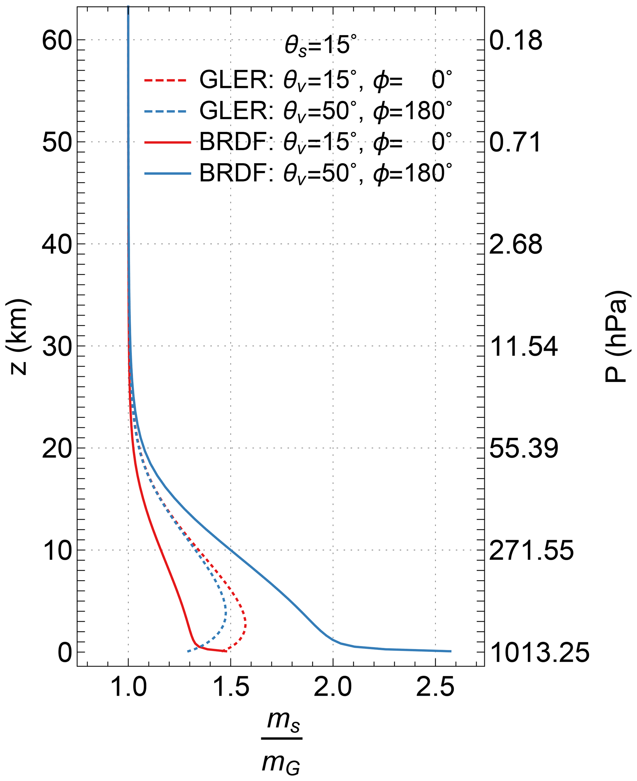
Figure 5 Mean path lengths (m_s) of EPIC band 1 reflective photons from an ocean surface (with the same BRDF described in Fig. 4) and its Lambertian equivalent surfaces. Here the mean path lengths m_s, normalized by the respective geometric air mass factors (m_G), are plotted as functions of altitude z for two viewing illumination geometries: one view from the direction of specular reflection at ${\mathit{\theta }}_{\mathrm{v}}=\mathrm{15}{}^{\circ }$ and $\mathit{\varphi }=\mathrm{180}{}^{\circ }$ and the other at ${\mathit{\theta }}_{\mathrm{v}}=\mathrm{50}{}^{\circ }$ and $\mathit{\varphi }=\mathrm{0}{}^{\circ }$, while the Sun is at ${\mathit{\theta }}_{\mathrm{s}}=\mathrm{15}{}^{\circ }$ for both geometries.

As described above, UV reflectivities for most natural surfaces are quite low (GLER <0.1); therefore, the surface contributions I_s are typically much smaller than (<10 % at 317.5 nm) the path radiance I_a (see Fig. 6). In modeling a measured radiance I_M, an error in surface radiance I_s is compensated for with the path radiance I_a. The uncertainty of extrapolated GLER is usually less than 1 %, corresponding to a less than 1 % error in I_s and hence less than 0.1 % error in the path radiance I_a. Furthermore, the AMF error due to the Lambertian treatment of an anisotropic surface is insignificant, since the combined mean photon path lengths,

$$\begin{array}{}\text{(7)}& m_z=-\partial \ln I_{\mathrm{TOA}}/\partial {\mathit{\tau }}_z=(I_{\mathrm{a}}{m}_{\mathrm{a}}+I_{\mathrm{s}}{m}_{\mathrm{s}})/I_{\mathrm{TOA}},\end{array}$$

contain minor contributions from surface radiance I_s.

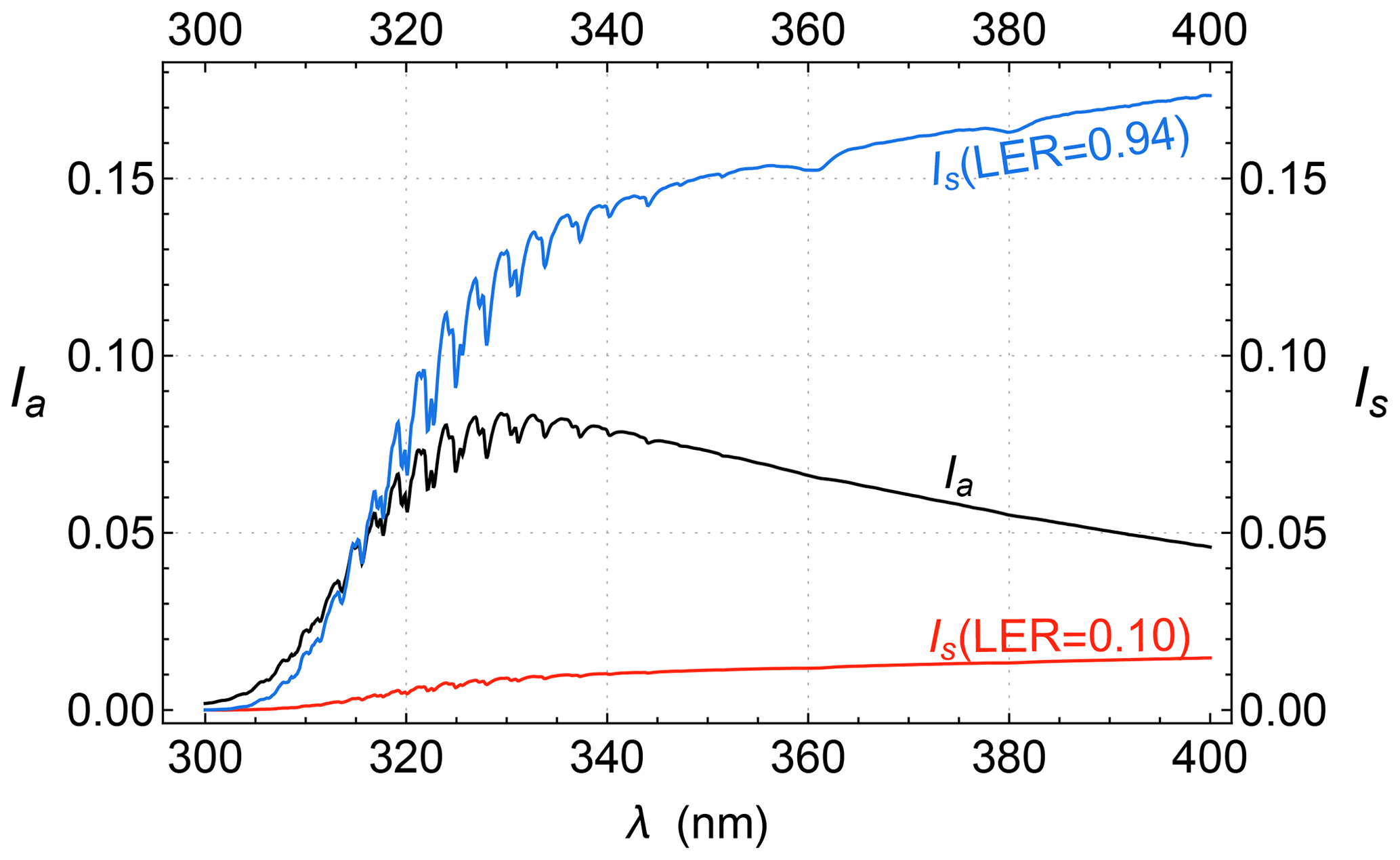
Figure 6 Example path radiance, I_a, and surface radiance I_s for ${\mathit{\theta }}_{\mathrm{s}}=\mathrm{45}{}^{\circ }$, ${\mathit{\theta }}_{\mathrm{v}}=\mathrm{40}{}^{\circ }$, and $\mathit{\varphi }=\mathrm{135}{}^{\circ }$. I_a is the middle line in black, and I_s for LER =0.1 and LER =0.94 is represented by the lower (red) and upper (blue) lines, respectively.

Natural surfaces with high UV reflectivities (GLER >0.2) are surfaces covered with snow, ice, or both. The highest GLER values are found over Antarctica and Greenland, where typical GLER values are higher than 0.9, as shown in Fig. 7. Figure 7 shows sample results of a climatological GLER database for Antarctic ice constructed from the observations of polar-orbiting instruments, including Aura OMI and SNPP OMPS, and it reveals a sizable dependence of ice GLER values on the viewing illumination geometry, indicating that the reflection from ice is significantly anisotropic. Because of the much higher surface radiance I_s (e.g., Fig. 6 blue line), the Lambertian treatment of ice surface can lead to large AMF errors. However, the ice GLER varies within a small range (0.94 to 0.98), and hence ice reflection has weak anisotropy for low SZA and VZA ($<\mathrm{70}{}^{\circ }$). Because the stronger O₃ absorption and Rayleigh scattering at shorter wavelengths reduce the fraction of direct solar beam but increase that of the diffuse radiation reaching the surface, further weakening the BRDF effect, the error of Lambertian treatment of ice surface in the sampling of atmospheric O₃ absorption is suppressed for the low SZA and VZA observations.

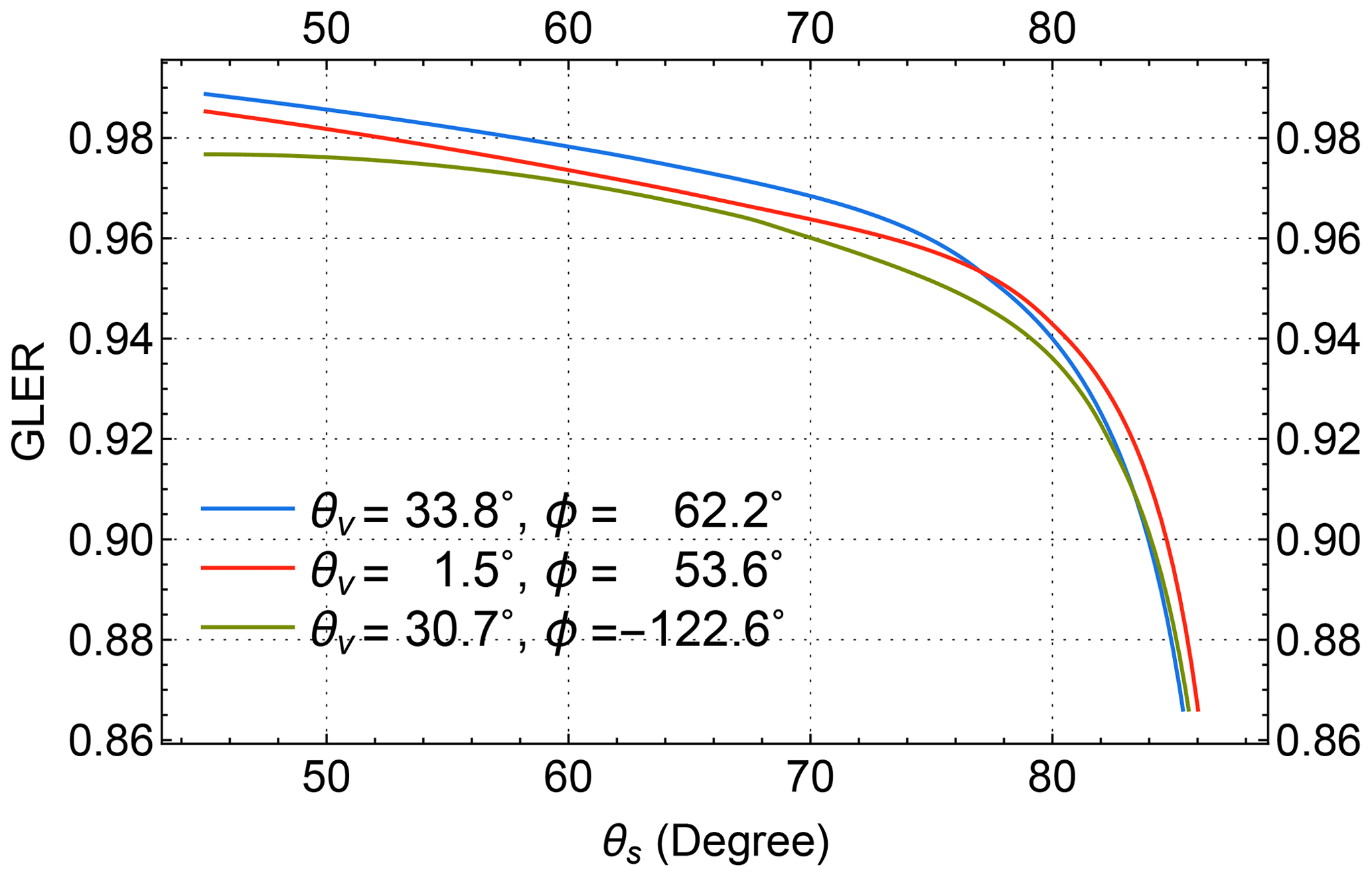
Figure 7 Climatological Antarctic GLER values at 331 nm as functions of SZA (θ_s) for three viewing geometries, revealing a significant dependence of ice GLER on the viewing illumination geometry.

2.3 Particle scattering and absorption

Atmospheric particles, including clouds and aerosols, reside mostly in the troposphere and cover a large portion (∼67 % by clouds alone; King et al., 2013) of the Earth's surface. Radiative transfer modeling of sunlight through a particle-laden atmosphere can be performed to quantify the TOA contributions from possible light paths, provided that the optical (scattering and absorption) properties of these particles, their amounts, and vertical distributions are specified. However, for UV remote sensing observations, the quantitative information about particles needed for radiative transfer modeling is in general not sufficiently known, precluding their explicit treatment. In this section, we describe an implicit treatment of atmospheric particles for the simulation of measured radiances with the mean photon path approximately matching that through the particle-laden atmosphere.

Atmospheric particles scatter and possibly absorb UV photons; they can thus significantly alter their paths through layers from closely above the particles down to the ground surface, usually shortening the path lengths below while lengthening those above the particles. Observing from space, the apparent effect of atmospheric particles is the enhancement of the TOA radiance contributed by backscattering from them. Since this effect is very similar to the consequence of an increased surface albedo, it is often referred to as the albedo effect. The albedo effect can be modeled by placing in a molecular atmosphere an elevated bright surface that partially covers an IFOV. This treatment is called the mixed Lambertian equivalent reflectivity (MLER) model, which is frequently employed by many algorithms for trace gas retrievals. Based on the MLER model, the TOA radiance for an IFOV is expressed as

$$\begin{array}{}\text{(8)}& I_{\mathrm{TOA}}=I_g(R_g,p_g)(\mathrm{1}-f_{\mathrm{c}})+I_{\mathrm{c}}(R_{\mathrm{c}},p_{\mathrm{c}})f_{\mathrm{c}},\end{array}$$

the weighted sum of two independent contributions I_g and I_c. Here I_g is the radiance from the cloud-free portion of the IFOV containing a Lambertian surface of reflectivity R_g at pressure p_g. Similarly, I_c is from the cloudy portion, and f_c is the cloud fraction and R_c the reflectivity of the Lambertian surface at pressure p_c.

The MLER model can reproduce measured radiances I_m through the determination of cloud fraction f_c. First, the scene LER r_s at surface pressure p_g is estimated using Eq. (6). If r_s is less than or equal to the climatological LER value R_g (e.g., Kleipool et al., 2008), this IFOV is treated as a particle-free scene (f_c=0). If r_s is greater than or equal to the LER value for cloud R_c=0.8 (Koelemeijer and Stammes, 1999; Ahmad et al., 2004), this IFOV is treated as fully cloud-covered (f_c=1). When r_s is between R_g and R_c, the cloud fraction is inverted from Eq. (8), which yields

$$\begin{array}{}\text{(9)}& f_{\mathrm{c}}={\displaystyle \frac{I_{\mathrm{M}}-I_g}{I_{\mathrm{c}}-I_g}}.\end{array}$$

In the case of f_c=0 or 1, surface LER r_g or cloud LER r_c is determined using Eq. (6) to ensure that modeled radiance I_TOA is equal to the measurement I_M. Figure 8 shows cloud fractions (f_c) as a function of wavelength for several examples of particle-laden atmospheres.

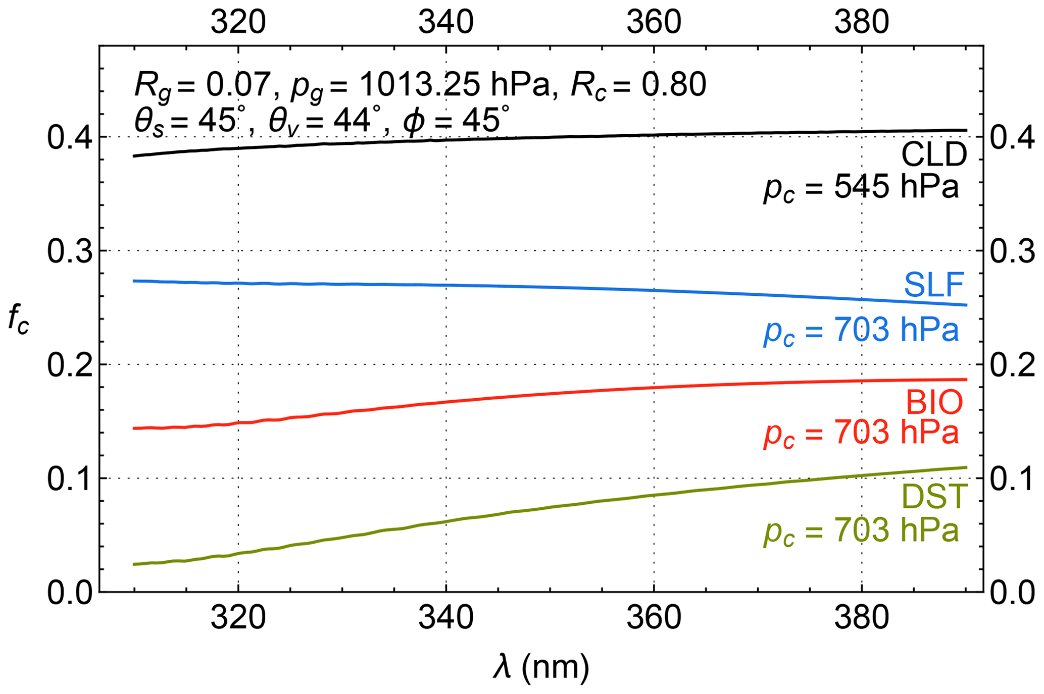
Figure 8 Four examples of cloud fractions (f_c) derived from explicitly modeled TOA radiances for particle-laden atmospheres. The first of these is the atmosphere with a 1.5 km thick layer of C1 cloud (CLD; Deirmendjian, 1969) with a single-scattering albedo ω=1 and an optical thickness τ=5 at 340 nm centered at 5 km altitude (or pressure level of 545 hPa). The others are atmospheres with a 1 km thick layer of aerosols, including SLF (ω=0.996), BIO (ω=0.921), and DST (ω=0.900) aerosols (SLF, BIO, and DST models are taken from Torres et al., 2007), with an optical thickness τ=1.5 at 340 nm centered at 3 km altitude (or pressure level of 703 hPa). The insets list the MLER parameters, R_g, p_g, R_c, and p_c, as well as the angles (θ_s, θ_v, and ϕ) that specify the viewing illumination geometry.

The radiance intensity scattered from atmospheric particles varies smoothly with wavelength without high-frequency spectral structures. For instance, the contributions to TOA radiances (I_TOA) from backscattering by meteorological clouds change smoothly and slowly with wavelength (see Fig. 8, the CLD curve). The selection of R_c=0.8 facilitates close simulation of the spectral variation of clouds observed from space (Ahmad et al., 2004) by the MLER model such that retrieved f_c has a small spectral variation (i.e., f_c nearly the same for different wavelengths) for most cloudy observations. The small and smooth change of f_c with wavelengths allows its extrapolation to provide a reliable estimate of f_c at shorter wavelengths from those determined at longer wavelengths.

Certain types of aerosols, such as continental aerosols containing soot, smoke from fires, mineral dust from deserts, and ash from volcanic eruptions, both scatter and absorb UV photons passing through them. Usually, aerosol absorptions cause the underlying surface (including clouds) to appear darker, more so at shorter wavelengths. The change in I_TOA due to the addition of aerosols and hence the cloud fraction (f_c or the surface LER, r_g) are smooth in wavelength (see, e.g., Fig. 8, with smooth curves for weakly absorbing sulfate-based aerosols – SLFs, carbonaceous aerosols from biomass burning – BIO, and mineral dust – DST; Torres et al., 2007). Therefore, f_c (when f_c>0, from Eq. 9) or r_g (when f_c=0, from Eq. 6) determined at longer wavelengths where atmospheric absorption is weak may be linearly extrapolated to O₃-sensitive wavelengths for estimation of contributions to TOA radiance from surface reflection and particle backscattering (referred to as the r_gf_c extrapolation method hereafter).

The UV aerosol index (AI; Herman et al., 1997; Torres et al., 1998), which measures the deviation of the spectral variation of TOA radiance from that of a pure molecular atmosphere, is proportional to the spectral slope c_l used in the r_gf_c extrapolation scheme. Algebraically, AI is calculated as the N-value (defined as −100log ₁₀I) difference between the modeled (I_TOA) and measured (I_M) radiances at a wavelength λ.

$$\begin{array}{}\text{(10)}& {\displaystyle }\mathrm{AI}& {\displaystyle }=\mathrm{100}{\log }_{\mathrm{10}}{\displaystyle \frac{I_{\mathrm{M}}\left(\mathit{\lambda }\right)}{I_{\mathrm{TOA}}\left(\mathit{\lambda },R_{\mathrm{e}}\right)}}\text{(11)}& {\displaystyle }& {\displaystyle }=\mathrm{100}{c}_l\mathrm{\Delta }\mathit{\lambda }{\displaystyle \frac{\partial {\log }_{\mathrm{10}}{I}_{\mathrm{TOA}}\left(\mathit{\lambda },R\right)}{\partial R}}{|}_{R=R_{\mathrm{e}}}\end{array}$$

Here, the modeled radiance I_TOA(λ,R_e) is calculated for a molecular atmosphere with an estimated reflectivity parameter R_e, which may be the LER value r_s or the MLER cloud fraction f_c determined at a well-separated wavelength (λ+Δλ). The pair of wavelengths used for the AI calculation is in the UV spectral range with weak molecular absorption, and their separation Δλ should be sufficiently large (>10 nm) to capture the spectral contrast of Rayleigh scattering. Using $I_{\mathrm{M}}\left(\mathit{\lambda }\right)=I_{\mathrm{TOA}}(\mathit{\lambda },R_{\mathrm{m}})=I_{\mathrm{TOA}}(\mathit{\lambda },R_{\mathrm{e}}+\mathrm{\Delta }R)$, since the reflectivity parameter R_m is derived from I_M(λ) and $\mathrm{\Delta }R=R_{\mathrm{m}}-R_{\mathrm{e}}=c_l\mathrm{\Delta }\mathit{\lambda }$, we arrive at Eq. (11) from the definition of AI in Eq. (10). In short, the spectral slope c_l is equivalent to the AI, which is significantly positive for particles (such as smoke, dust, and volcanic ash) with large absorption and slightly positive to negative for non-absorbing and weakly absorbing particles (such as clouds and sulfate aerosols). Note that for the conventional AI (also called LER AI) calculation, radiance I_TOA is modeled for a Rayleigh-scattering-only atmosphere over a Lambertian surface. To capture the spectral slope of the r_sf_c extrapolation scheme, we switch the LER treatment with the MLER modeling of I_TOA for AI calculation. The resulting MLER AI is usually higher than the corresponding LER AI when f_c>0, but otherwise it can be similarly used to indicate the presence of UV-absorbing aerosol.

The MLER treatment enables the modeling of measured radiances without knowledge of the optical properties or the full vertical distributions of atmospheric particles. The accuracy of the modeled radiances at the extrapolated wavelengths depends on how closely the MLER parameter (r_g or f_c) follows the linear relationship among different wavelengths. In reality, the spectral dependence of natural surface reflection (r_g) or particle scattering and absorption (f_c) is nonlinear, though moderately as exemplified in Figs. 4b and 8. Therefore, r_gf_c extrapolation yields small errors in r_g or f_c at the extrapolated wavelengths. The radiance uncertainties associated with the r_gf_c extrapolation error are below 1 % for the vast majority of remote sensing observations. Higher radiance uncertainties usually occur in the presence of highly elevated or strongly absorbing aerosols. These observations may be flagged with high AI values.

In addition to the mostly small radiance errors at the extrapolated wavelengths, the MLER treatment can simulate the photon sampling of particle-laden atmospheres with a diverse range of particle types and vertical distributions. Figure 9 shows comparisons of mean photon path lengths of particle-laden atmospheres with those from the corresponding MLER treatments. These comparisons illustrate that the layer mean photon paths based on the MLER model deviate from those of the particle-laden atmospheres, mostly in the region immediately above the particles down to the underlying surface. These deviations diminish with higher altitudes where lower air density reduces the chance of photons being scattered. Since the vast majority of clouds and aerosols are in the lower troposphere ($<\sim \mathrm{10}$ km), the MLER treatment does not introduce significant AMF errors in accounting for O₃ absorption, which occurs mostly in the stratosphere. This is similar to how the Lambertian treatment of surface reflection works for the estimation of total O₃ absorption (see Sect. 2.2).

Figure 9 Mean photon path lengths m_z, normalized by the geometric AMF m_G, of EPIC bands 1 and 2 as functions of altitude z for particle-laden atmospheres and their MLER treatments. See the caption of Fig. 8 for the description of aerosol characterizations, MLER treatments, and the viewing illumination geometry.

The MLER treatment relies on a few adjustable parameters, including the cloud fraction f_c and cloud pressure p_c, to model a vast range of conditions encountered in remote sensing of Earth's atmosphere. The cloud fraction f_c, obtained directly from radiance measurements using Eq. (9), provides an estimate of the cloud amount in an IFOV. The pressure p_c of the elevated Lambertian surface needs to be set at a proper level to best approximate the layer mean photon paths of a particle-laden atmosphere. As seen in Fig. 9, the optimal placement of the elevated Lambertian surface is within the particle layer, as p_c located too high or too low from the optical centroid pressure (OCP; Joiner and Vasilkov, 2006; Vasilkov et al., 2008) would make layer mean photon paths deviate further from those of the particle-laden atmosphere. The effective cloud pressures retrieved from the EPIC measurements of the O₂ A band (Yang et al., 2019) are usually located within the particle vertical distributions and therefore used to set the cloud pressures p_c for processing EPIC observations.

The use of OCP for p_c enables the MLER model to account for the measurement sensitivity change when a layer of particles is introduced into the atmosphere: enhancing the photon attenuation by absorbers inside and above the layer, while reducing them below, as the mean photon paths or AMFs from the MLER model lengthen above p_c but shorten below it, as illustrated in Fig. 9. Since the MLER model captures the enhancement and shielding effects on trace gas absorption by atmospheric particles, it is widely adopted due to its simplicity for retrievals of trace gases besides O₃, such as NO₂ and SO₂ in the troposphere. However, sizable AMF errors are prevalent for modeling tropospheric absorptions based on the MLER treatment, which usually yields significantly different mean photon paths from those of explicit treatment in the troposphere.

2.4 Inelastic molecular scattering

The scattering of sunlight with atmospheric constituents is mostly elastic; i.e., the energy and thus the wavelength of a photon remain the same before and after the interaction. But a small portion (∼4 %) of molecular scattering is inelastic, resulting in energy gain or loss of the scattered photons. Specifically, the rotational Raman scattering (RRS) from air molecules (such as nitrogen and oxygen) can alter the wavelengths of scattered photons, with UV wavelength shifts $\mathrm{\Delta }\mathit{\lambda }<\pm \mathrm{2}$ nm (Joiner et al., 1995; Chance and Spurr, 1997; Vountas et al., 1998). These inelastic scatterings cause the filling-in of telluric lines (i.e., trace gas absorption features) and solar Fraunhofer lines (also known as the Ring effect, which was first noticed by Grainger and Ring, 1962).

The filling-in effect is a function of wavelength and depends on the optical properties of the atmosphere, the viewing and illumination geometry, and the surface reflectivity and pressure. The filling-in effect also depends on the ISRF, especially on the instrument spectral resolution, which is the width of its ISRF, since the measured radiance of a band is a convolution of spectral radiance and the ISRF (see Eq. 1). This effect is quantified with the filling-in factors, defined as $\mathit{\varrho }=(I_{\mathrm{RRS}}-I_{\mathrm{ELA}})/I_{\mathrm{ELA}}$, where I_ELA is the TOA radiance calculated assuming all molecular scattering is elastic, while I_RRS includes the inelastic (RRS) contributions. To illustrate the significance of RRS, we show in Fig. 10 examples of the filling-in factors, calculated for EPIC bands using the scalar LIDORT-RRS radiative transfer code (Spurr et al., 2008). Since RRS is weakly dependent on polarization, a scalar radiative transfer model, from which both I_ELA and I_RRS are calculated without including radiation polarization, can accurately provide filling-in factors (Landgraf et al., 2004; Wagner et al., 2010).

The filling-in factors provide estimates of the modeling errors in I_TOA when RRS contributions are neglected, and results in Fig. 10 show variations of modeling errors with different observing conditions. These errors are usually systematic for a spectral band and are between 0.5 and 1 % for measurements of EPIC bands 1 and 2. These errors are sufficiently large that corrections are required for achieving high (∼1 %) O₃ retrieval accuracy. The filling-in factors (ϱ), modeled using a scaler code (like LIDORT-RRS), may be used to correct the results (I_TOA) from vector radiative transfer codes (e.g., Dave, 1964; Spurr, 2006) that perform elastic modeling only, i.e., the RRS-corrected TOA radiance $=I_{\mathrm{TOA}}(\mathit{\varrho }+\mathrm{1})$.

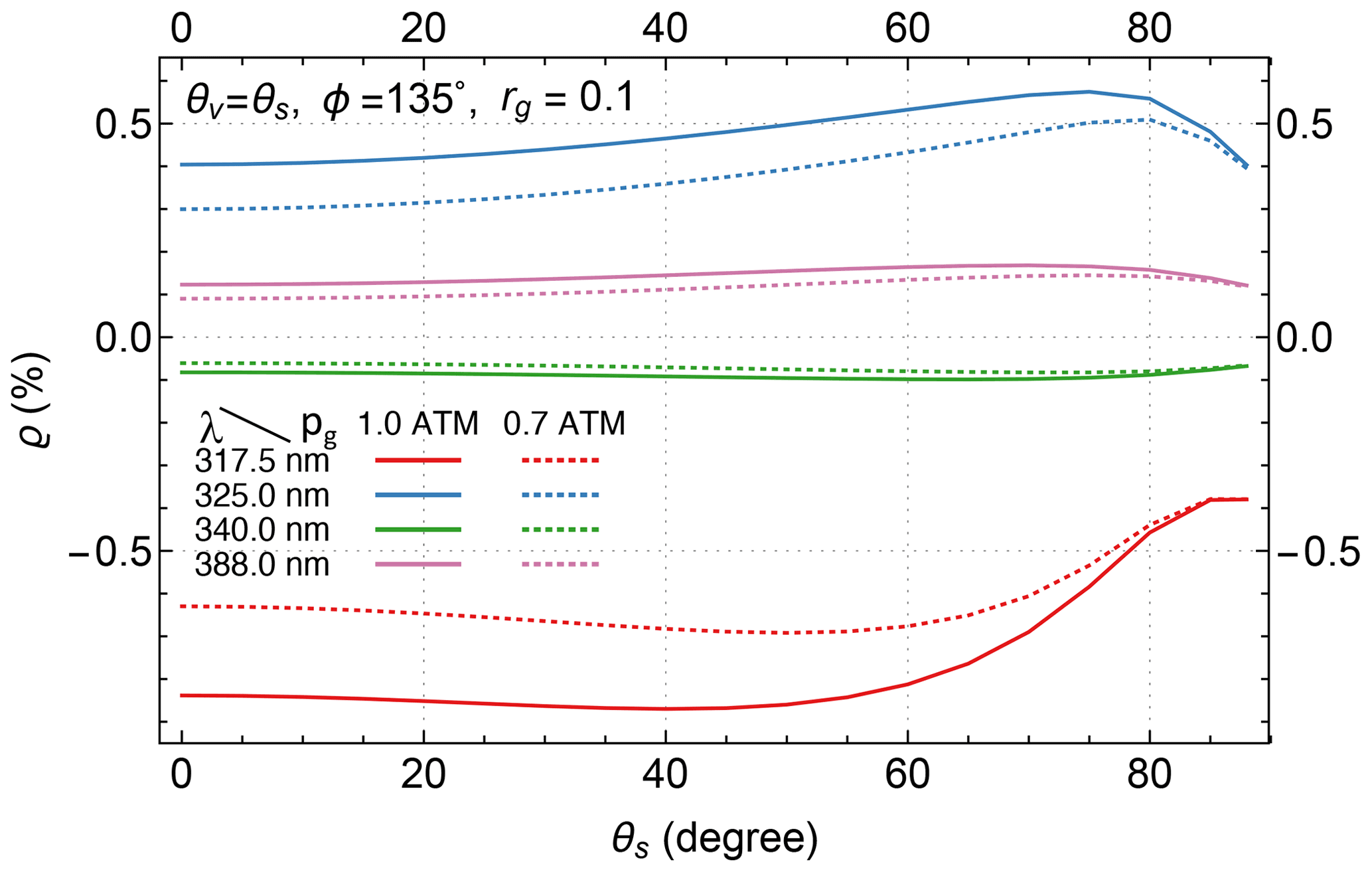
Figure 10 Filling-in factors $\left(\mathit{\varrho }=\frac{I_{\mathrm{RRS}}-I_{\mathrm{ELA}}}{I_{\mathrm{ELA}}}\times \mathrm{100}\right)$ for EPIC UV bands as a function zenith angle at two surface pressures p_g=0.7 ATM and p_g=1.0 ATM, with a surface albedo of r_g=0.1.

3 O₃ and temperature vertical profiles

As shown in Sect. 2.1, the O₃ vertical distribution or profile directly affects the magnitude of a measured radiance in the spectral region with significant O₃ absorption. Hence, the interpretation of radiance change due to O₃ absorption requires some knowledge of its profile. In general, the retrieval of quantitative information about a gaseous absorber (such as O₃ and SO₂) requires a model to prescribe its vertical distribution. The skill of this model in representing the actual vertical distribution of the absorber significantly contributes to the quantification accuracy. In this section, we describe a recently developed O₃ profile model for remote sensing retrieval algorithms and its improvements over the model commonly used by other total O₃ algorithms.

Ozone is naturally present throughout the atmosphere, and its spatial and temporal distribution is controlled by atmospheric processes of O₃ production, destruction, and transport. The O₃ distribution exhibits a high abundance of O₃ in the stratosphere and a minor portion (∼10 %) in the troposphere, with the peak O₃ concentration occurring at a lower altitude as the latitude increases towards the poles. These characteristics are well-captured by O₃ profile climatologies (e.g., Fortuin and Kelder, 1998; McPeters et al., 2007; McPeters and Labow, 2012), which provide the mean and variance of O₃ vertical distribution as a function of latitude and calendar month. These climatologies also reveal that the O₃ profile has the highest variability in the upper troposphere and lower stratosphere (UTLS), contributing the most to the natural variations in total O₃. This high O₃ variability is the consequence of atmospheric movements that blend air masses with different O₃ concentrations, such as uplifting of O₃-poor air in the troposphere or lowering of O₃-rich air in the stratosphere resulting from the rise and fall of the tropopause. Predictors of O₃ profile shape, including tropopause pressure and total O₃ columns, are developed to capture the dynamical influences on O₃ vertical distributions, resulting in the construction of tropopause-sensitive (Wei et al., 2010; Bak et al., 2013; Sofieva et al., 2014) and total-column-dependent (Wellemeyer et al., 1997; Bhartia and Wellemeyer, 2002; Lamsal et al., 2004; Labow et al., 2015) O₃ profile climatologies.

The O₃ profile model for the Total Ozone Mapping Spectrometer Version 8 (TOMS-V8) total O₃ algorithm combines the latitude-dependent monthly mean Labow–Logan–McPeters (LLM) climatology (McPeters et al., 2007) with the latitude- and total-column-dependent annual mean climatology (Bhartia and Wellemeyer, 2002) to determine the O₃ profile as a function of latitude, time (day of year, DOY), and total O₃ column. This model has been adopted by nearly all the contemporary total O₃ algorithms (e.g., Bhartia and Wellemeyer, 2002; Eskes et al., 2005; Veefkind et al., 2006; Van Roozendael et al., 2006; Lerot et al., 2010; Loyola et al., 2011; Van Roozendael et al., 2012; Lerot et al., 2014; Wassmann et al., 2015) owing to its capability to characterize O₃ profile variation with the total column.

To improve the representation of the O₃ profile, we construct both tropopause-dependent and total-column-dependent climatologies using the Modern-Era Retrospective Analysis for Research and Applications Version 2 (MERRA-2; Bosilovich et al., 2015; Gelaro et al., 2017) O₃ record between 2005 and 2016. The total-column-dependent climatology, named M2TCO3, is more appropriate for use as the O₃ profile model needed by a total O₃ algorithm, as it is generally more reliable than the tropopause-dependent version in prescribing realistic O₃ profiles (Yang and Liu, 2019).

Figure 11 compares daytime M2TCO3 (Yang and Liu, 2019; referred to as M2TCO3 hereafter) and TOMS-V8 profiles for 2 months and four latitude zones, illustrating the similarities and differences between the two O₃ models. Both show north–south asymmetry, i.e., profiles in the Northern Hemisphere differ from those in the Southern Hemisphere for the corresponding months and latitude zones (e.g., September and 60–50^∘ S vs. March and 50–60^∘ N in Fig. 11), substantial seasonal variations (e.g., 60–50^∘ S, March vs. September in Fig. 11), a strong dependence on latitude exhibiting lower altitudes of O₃ concentration peaks at higher latitudes for similar total columns, and characteristic dependence on the total column, which gets smaller with a higher O₃ peak altitude (e.g., March and 50–60^∘ N in Fig. 11). Figure 11 shows good agreements of zonal mean profiles (e.g., close matches between solid black and dotted black curves in each panel of this figure) but significant differences between M2TCO3 and TOMS-V8 profiles for similar total columns. These differences are due to TOMS-V8's use of annual mean column-dependent climatology to account for profile variations with the total column throughout the year (Bhartia and Wellemeyer, 2002), thus ignoring the significant seasonal dependence. An additional deficiency of TOMS-V8 contributing to the differences is its inadequate representation of latitude-dependent O₃ profile variation with the total column, including broad (30^∘) latitude zones and omission of north–south asymmetry. These deficiencies are eliminated with M2TCO3, which improves the realism of O₃ profile representation.

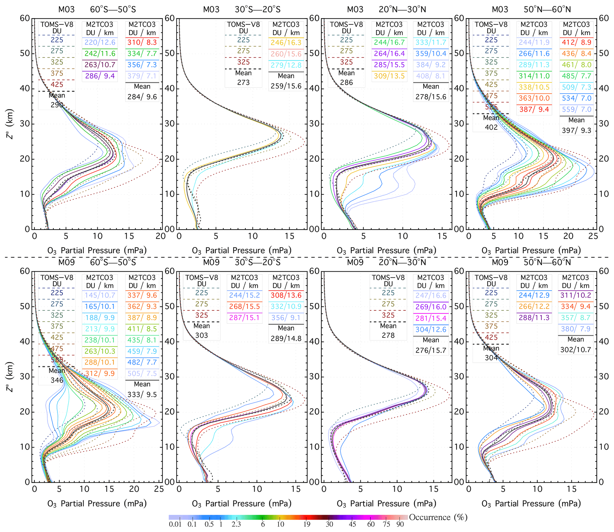
Figure 11 Profile comparisons between M2TCO3 and TOMS-V8 for 2 months (March and September) and four latitude zones: 60–50^∘ S, 30–20^∘ S, 20–30^∘ N, and 50–60^∘ N. Colored solid lines represent M2TCO3 profiles, while the dotted ones are for TOMS-V8 profiles. The color of a solid line indicates the percentage occurrence of the climatological profile, and its line legend displays the mean tropopause altitude and the mean total column O₃ of the profile. The solid black lines represent the downgraded M2TCO3 (i.e., the monthly zonal mean) profiles, and dotted lines are TOMS-V8 monthly zonal mean (i.e., the LLM climatological) profiles. Here pressure altitude is defined as $Z^{*}=\mathrm{16}{\log }_{\mathrm{10}}\left[\frac{p_{\mathrm{s}}}{p}\right]$, where p is pressure level (in hPa) and p_s=1013.25 hPa.

In short, M2TCO3 better captures the dynamical changes and spatiotemporal variations in O₃ profiles with higher resolutions in total O₃ column (25 DU), latitude (10^∘), and time (monthly). Taking into account the substantial change in atmospheric O₃ over a long time, M2TCO3 is more accurate in representing atmospheric O₃ vertical distribution from the recent past to near future than the TOMS-V8 model, which was compiled from earlier satellite and ozonesonde data (mostly from the 1980s and 1990s; Wellemeyer et al., 1997; McPeters et al., 2007). Hence, we use the M2TCO3 climatology as the O₃ profile model for total O₃ retrieval from EPIC.

The M2TCO3 climatology contains not only mean profiles that represent the likely O₃ vertical distributions, but also the modal O₃ adjustment profiles that specify the probable deviations from the means. These modal profiles are determined from the O₃ profile covariance statistics, as illustrated in Fig. 12, showing examples of M2TCO3 climatological O₃ profiles and the associated modal profiles, which are the eigenvectors (also known as the empirical orthogonal functions or EOFs) of the profile covariance matrices. Algebraically the representation of an O₃ profile X is expressed as

$$\begin{array}{}\text{(12)}& \mathbf{X}={\mathbf{X}}_{\mathrm{m}}\left(v\right)+\sum _{k=\mathrm{1}}^p{\mathit{\gamma }}_k{e}_k\left(v\right),\end{array}$$

where X_m(v) is a climatological profile that depends on a set of variables v, which for M2TCO3 consists of the total column (Ω₀), time, and location. e_k(v) is the kth modal profile, γ_k the kth coefficient, and p the number of e_k(v), with a maximum equal to the number of levels used to represent an O₃ profile in the climatology. Usually, a few modal profiles are sufficient to account for the majority of profile variance. For example, in Fig. 12, the first five EOFs (panels b and e) of the covariance matrices (panels c and f) account for 80 % of profile variances (blue shaded area in panels a and d). An actual O₃ profile X, which deviates invariably from the mean X_m, can be accurately represented using Eq. (12) with a small number of expansion coefficients γ_k. Much like the mean the profile X_m represents the most probable vertical distribution of O₃: the modal profiles, $\mathit{\{}{e}_k,k=\mathrm{1}\mathrm{\dots }\mathit{\}}$, describe the most, the second most, and so on likely vertical patterns of deviations from the mean profile. Each modal profile describes a rearrangement, like shifting, shrinking, or broadening, of the mean profile without substantially changing the total column. With these modal profiles constraining how a profile can be adjusted, the retrieval algorithm can exploit the O₃ profile information contained in multi-spectral measurements to improve the O₃ profile representation by determining one or more linear expansion coefficients {${\mathit{\gamma }}_k,k=\mathrm{1}\mathrm{\dots }$}. Note that for most total ozone algorithms, the O₃ profile representation is limited to the climatological mean only, equivalent to restricting γ_k=0 for all k in Eq. (12).

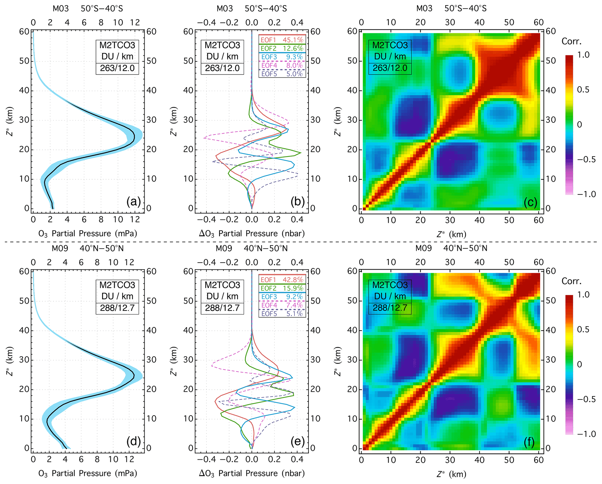
Figure 12 Examples of M2TCO3 climatological profiles for the southern midlatitude zone in March (a) and the northern midlatitude zone in September (b), the associated correlation matrices (c, f), and the corresponding modal O₃ profiles (b, e). The blue shaded areas in panels (a) and (d) are within 1 standard deviation of the mean. The correlation matrices in (c) and (f) are standardized (i.e., diagonal element normalized to 1) covariance matrices. The five modal profiles in (b) and (e) are the first five ordered eigenvectors (also known as empirical orthogonal functions or EOFs) of the corresponding covariance matrices, with percentages of the profile variance explained by the EOFs displayed in the line legends. The text box in each panel displays the average tropopause altitude (in km) and the average total O₃ column (in DU) for the climatological profile.

The total column is a good predictor of an O₃ profile that is especially accurate for the shape in the stratosphere but less so in the troposphere. Tropospheric O₃ exhibits characteristic spatiotemporal distribution, which is captured in the MERRA-2 tropospheric O₃ climatology (Yang and Liu, 2019). To better represent the O₃ profile, the tropospheric part of a column-dependent M2TCO3 profile, X_m, is scaled with the ratio of the MERRA-2 climatological tropospheric column to the tropospheric column integrated from the downgraded M2TCO3 profile (see Fig. 11 for sample M2TCO3 and downgraded M2TCO3 profiles). In other words, the profile X_m in Eq. (12) has its tropospheric part tied to the spatiotemporally varying climatological tropospheric column, to which the tropospheric column of the mean X_m profile (obtained by averaging over the different column amounts) is matched.

In addition to knowledge of profiles of light-absorbing trace gases, such as O₃ and SO₂, radiative transfer modeling of measured radiance requires knowledge of the atmospheric temperature profile because the absorption cross-sections of these trace gases significantly depend on temperature. For total O₃ retrieval from EPIC, this knowledge is taken from the temperature profile climatology created from MERRA-2 data together with the ozone profile climatology (Yang and Liu, 2019). This temperature climatology provides mean temperature profiles corresponding to the climatological O₃ profiles, capturing the dependence of the temperature profile on season and location, as well as the variation of temperature with the O₃ profile. It is an improvement over the TOMS-V8 temperature profile climatology, which provides latitude- and month-dependent temperature profiles, but without accounting for the strong correlation between temperature and O₃ profiles.

4 Inversion technique

Section 2 describes algorithm physics treatments of interactions of solar radiation with atmospheric particles and surfaces to enable RT modeling of photons traversing through a molecular atmosphere to reproduce the measured TOA radiances with photons that follow the paths similar to those through the actual atmosphere and therefore establish the relationship between spectral measurements and the atmospheric state, as well as surface reflectivity and instrumental parameters. At its core, the RT modeling sets up a forward mapping from the vertical distributions of gaseous absorbers and the surface reflectivity parameters to measured TOA radiances. The retrieval of gas absorbers, such as O₃ and SO₂, is the inverse of this mapping, i.e., to find their vertical distributions and the surface reflectivity parameters for which forward modeling closely reproduces the measured TOA radiances. However, this inverse mapping is inherently an ill-posed problem, as the solution is not unique; i.e., more than one set of profiles and surface parameters can yield the same measurements. This problem is made worse with measurement uncertainties, which expand the profile and surface combinations that can reproduce, within error bars, the measured spectra.

For successful inversion, analytical constraints are placed on the profiles of gas absorbers as well as the spectral variations of ground reflectivity and atmospheric particle (aerosol and cloud) backscattering. For O₃ retrieval, Eq. (12) embodies the profile constraint, while the MLER model with r_sf_c extrapolation regulates the surface reflection and particle backscattering. These constraints control the dimension of the inverse mapping space and manifest themselves as the retrieval (i.e., adjustable) parameters, which, in the case of O₃ retrieval, consist of total O₃ column Ω, a number (p) of modal expansion coefficients $\mathit{\{}{\mathit{\gamma }}_k,k=\mathrm{1}\mathrm{\dots }p\mathit{\}}$, surface LER (r_s) or cloud fraction (f_c), and a number (q) of polynomial coefficients $\mathit{\{}{c}_l,l=\mathrm{1}\mathrm{\dots }q\mathit{\}}$ of the r_sf_c extrapolation. The set of adjustable parameters forms the state vector (x) whose length (n) is the dimension of inverse mapping space. Proper selection of adjustable parameters by limiting the number of modal coefficients (p≥0) and polynomial coefficients (q≤1) ensures that the inverse problem is well-posed and simultaneously maximizes the amount of information collected from the spectral measurements. Here p=0 indicates no modal expansion, equivalent to restricting the profile to a climatological column-dependent O₃ profile, and q=0 for the spectral invariant reflectivity parameter.

4.1 Exact solution

Conceptually, the inversion is to find the state vector (x) that satisfies a set of m simultaneous equations, $\mathit{\{}\mathrm{\Delta }{y}_i=\mathrm{0},i=\mathrm{1}\mathrm{\dots }m\mathit{\}}$, one for each spectral band difference, $\mathrm{\Delta }{y}_i=\ln I_{\mathrm{M}}\left({\mathit{\lambda }}_i\right)-\ln I_{\mathrm{TOA}}(\mathit{x},{\mathit{\lambda }}_i)$, between the radiance measurement I_M and the forward modeling I_TOA: here λ_i the wavelength that characterizes the ith ($\mathrm{1}\le i\le m$) spectral band and Δy_i the residual of this band. In matrix form, the m simultaneous equations can be expressed as

$$\begin{array}{}\text{(13)}& \mathrm{\Delta }\mathit{y}=\mathrm{0},\end{array}$$

where Δy is residual column vector $\mathit{\{}\mathrm{\Delta }{y}_i,i=\mathrm{1}\mathrm{\dots }m\mathit{\}}$. Since the forward mapping I_TOA(x) is a nonlinear function of the state vector x and has no analytical inverse, the solution to Eq. (13) is usually obtained iteratively. The iteration is started with an initial (i.e., iteration number L =0) state vector x_L to linearize the equation between residuals and the state vector.

$$\begin{array}{}\text{(14)}& \begin{array}{rl}\mathrm{\Delta }{y}_i=& \ln I_{\mathrm{M}}\left({\mathit{\lambda }}_i\right)-\ln I_{\mathrm{TOA}}\left({\mathit{x}}_{\mathrm{L}},{\mathit{\lambda }}_i\right)-\sum _{j=\mathrm{1}}^n\left(\mathit{x}{}_j-{\mathit{x}}_{\mathrm{L}}{}_j\right)\\ & {\displaystyle \frac{\partial \ln I_{\mathrm{TOA}}\left(\mathit{x},{\mathit{\lambda }}_i\right)}{\partial {\mathit{x}}_j}}{|}_{\mathit{x}={\mathit{x}}_{\mathrm{L}}},\end{array}\end{array}$$

where x_j and x_Lj are the jth components of x and x_L, respectively, $\mathrm{\Delta }{\mathit{x}}_j={\mathit{x}}_j-{\mathit{x}}_{\mathrm{L}}{}_j$ the jth components of state adjustment vector, and $K_{ij}=\frac{\partial \ln I_{\mathrm{TOA}}\left(\mathit{x},{\mathit{\lambda }}_i\right)}{\partial {\mathit{x}}_j}{\mathrm{|}}_{\mathit{x}={\mathit{x}}_{\mathrm{L}}}$ the Jacobian, also known as the weighting function for the retrieval parameter x_j at spectral band λ_i. The m residual elements, each written in Eq. (14), can be expressed in matrix form as

$$\begin{array}{}\text{(15)}& \mathrm{\Delta }\mathit{y}=\mathrm{\Delta }{\mathit{y}}_{\mathrm{L}}-\mathbf{K}\mathrm{\Delta }\mathit{x},\end{array}$$

where Δy_L is the column vector $\mathit{\left\{}\ln I_{\mathrm{M}}\right({\mathit{\lambda }}_i)-\ln I_{\mathrm{TOA}}({\mathit{x}}_{\mathrm{L}},{\mathit{\lambda }}_i),i=\mathrm{1}\mathrm{\dots }m\mathit{\}}$, $\mathrm{\Delta }\mathit{x}=\mathit{x}-{\mathit{x}}_{\mathrm{L}}$ the state adjustment vector, and K the m×n Jacobian matrix with the $\mathit{\{}{K}_{ij},i=\mathrm{1}\mathrm{\dots }m,j=\mathrm{1}\mathrm{\dots }n\mathit{\}}$ as its elements. Putting Eq. (15) into Eq. (13) yields

$$\begin{array}{}\text{(16)}& \mathrm{\Delta }{\mathit{y}}_{\mathrm{L}}=\mathbf{K}\mathrm{\Delta }\mathit{x},\end{array}$$

which may be solved exactly (under strict conditions) to determine the state adjustment vector Δx. After each iteration, the linearization state vector is updated to

$$\begin{array}{}\text{(17)}& {\mathit{x}}_{\mathrm{L}+\mathrm{1}}={\mathit{x}}_{\mathrm{L}}+\mathrm{\Delta }\mathit{x}.\end{array}$$

The final state x is found when the iteration converges, i.e., when the absolute change in state vector Δx is below a threshold.

The linear equation (Eq. 16) may be solved exactly only when the number of measurements is equal to the number of retrieval parameters (i.e., m=n) and the Jacobian matrix K is invertible (i.e., non-singular matrix), as exemplified in the well-known TOMS-V8 total O₃ algorithm (Bhartia and Wellemeyer, 2002). The TOMS-V8 algorithm determines the two-component state vector, $\mathit{x}=\mathit{\{}\mathrm{\Omega },r_{\mathrm{s}}\mathrm{or}{f}_{\mathrm{c}}\mathit{\}}$, from radiance measurements of two spectral bands: one with low O₃ sensitivity to estimate the MLER parameter (r_s or f_c) and the other with high O₃ sensitivity to derive total O₃ column Ω. However, few other algorithms adopt this inversion method, since it requires m=n and K to be a non-singular matrix. Even if both these conditions are met, inverting Eq. (16) to obtain exact solutions tends to enhance the impact of measurement uncertainties (noises) on the retrieved results, as in cases that K matrices are nearly but not quite singular. These cases occur when the spectral variation of a Jacobian has some similarity or a high degree of correlation with that of another retrieval parameter, leading to algorithm difficulty in distinguishing two retrieval parameters corresponding to the two Jacobians, thus yielding unstable retrieval results, such as in the case of simultaneous retrieval of total O₃ and SO₂ columns from EPIC UV measurements.

4.2 Direct fitting

Since spectral measurements have errors and m≠n in general, the inversion is achieved by finding the solution x that minimizes the cost function

$$\begin{array}{}\text{(18)}& {\displaystyle }\mathrm{{\rm Y}}\left(\mathit{x}\right)& {\displaystyle }=\Vert {\mathbf{S}}_{\mathit{ϵ}}^{-\frac{\mathrm{1}}{\mathrm{2}}}\mathrm{\Delta }\mathit{y}{\Vert }_{\mathrm{2}}^{\mathrm{2}}=\mathrm{\Delta }{\mathit{y}}^T{\mathbf{S}}_{\mathit{ϵ}}^{-\mathrm{1}}\mathrm{\Delta }\mathit{y}\text{(19)}& {\displaystyle }& {\displaystyle }=\sum _{i=\mathrm{1}}^m{\left({\displaystyle \frac{\mathrm{\Delta }{y}_i}{{\mathit{\mu }}_i}}\right)}^{\mathrm{2}},\end{array}$$

where S_ϵ is the measurement error covariance matrix, with its ith diagonal element equal to ${\mathit{\mu }}_i^{\mathrm{2}}$. Here μ_i is the fractional standard deviation of the radiance error of the ith band. In the case of independent measurement error, i.e., no error correlation between different spectral bands, Eq. (18) can then be explicitly written as Eq. (19), which is the formulation of the least-squares method.

The minimization of the cost function Υ can be started by linearizing the residuals with an initial (i.e., iteration number L =0) state vector x_L. Substituting Δy (Eq. 15) into Eq. (18), we minimize this cost function to obtain the state adjustment vector

$$\begin{array}{}\text{(20)}& \mathrm{\Delta }\mathit{x}=({\mathbf{K}}^T{\mathbf{S}}_{\mathit{ϵ}}^{-\mathrm{1}}\mathbf{K}{)}^{-\mathrm{1}}{\mathbf{K}}^T{\mathbf{S}}_{\mathit{ϵ}}^{-\mathrm{1}}\mathrm{\Delta }{\mathit{y}}_{\mathrm{L}}={\mathbf{G}}_{\mathrm{DF}}\mathrm{\Delta }{\mathit{y}}_{\mathrm{L}},\end{array}$$

which is the solution of linear weighted least-square regression. Here, ${\mathbf{G}}_{\mathrm{DF}}=({\mathbf{K}}^T{\mathbf{S}}_{\mathit{ϵ}}^{-\mathrm{1}}\mathbf{K}{)}^{-\mathrm{1}}{\mathbf{K}}^T{\mathbf{S}}_{\mathit{ϵ}}^{-\mathrm{1}}$ is the direct fitting (DF) gain matrix.

This procedure of iterative minimization of the difference between measurements and modelings to determine the bulk parameters is called the direct vertical column fitting (DVCF) algorithm. The DVCF algorithm is quite general and valid for both discrete wavelength and hyperspectral measurements, as well as for different types of retrieval parameters, such as MLER parameters, layer partial columns of various absorbing trace gases, and their total vertical columns. This algorithm has been applied to retrievals of total O₃ vertical column (Joiner and Bhartia, 1997; Yang et al., 2004; Lerot et al., 2014), the combination of total O₃ and SO₂ vertical columns (Yang et al., 2007, 2009a, 2013), the combination of O₃ and altitude-resolved SO₂ vertical columns (Yang et al., 2009b, 2010), and stratospheric and tropospheric NO₂ vertical columns (Yang et al., 2014). This algorithm is named DVCF to contrast with the DOAS (differential optical absorption spectroscopy) method (Platt, 2017), which derives a slant column and then uses an air mass factor (AMF) at a single wavelength (λ₀) to convert it to a vertical column.

In general, the DVCF algorithm works well when the changes in radiance measurements responding to changes in the state vectors are significantly different between any two retrieval parameters, i.e., that columns of K, which are the Jacobians of a retrieval parameter at different wavelengths, exhibit significantly different spectral dependence from one another. This is usually true for any two bulk retrieval parameters over a sufficiently broad spectral range, such as total O₃ column (Ω) and an expansion coefficient (γ_k) of differential profile e_k (see Eq. 12), or the SO₂ vertical column and its layer altitude. With measurements from a broad spectral range, the DVCF algorithm can discriminate subtle spectral features contained in hyperspectral measurements to enhance the retrieval accuracy (e.g., Yang et al., 2009b, 2010). Besides contrasting with the DOAS method, the name DVCF emphasizes the vertical column because this algorithm is usually not suitable for traditional profile retrieval due to the high similarity of partial column Jacobians between adjacent layers and hence the difficulty in distinguishing their partial columns.

4.3 Optimal estimation

In many cases, such as sparse spectral sampling or a narrow spectral range, the performance of the direct fitting inversion method may decline as a result of limited information contained in the spectral measurements. For stabilizing the retrieved results, the inversion process can be regulated with an additional constraint, which is frequently based on a priori knowledge of the retrieval parameters. Algebraically, adding an a priori constraint to Eq. (18) yields a new cost function

$$\begin{array}{}\text{(21)}& \mathrm{{\rm Y}}\left(\mathit{x}\right)=\mathrm{\Delta }{\mathit{y}}^T{\mathbf{S}}_{\mathit{ϵ}}^{-\mathrm{1}}\mathrm{\Delta }\mathit{y}+(\mathit{x}-{\mathit{x}}_{\mathrm{a}}{)}^T{\mathbf{S}}_{\mathrm{a}}^{-\mathrm{1}}(\mathit{x}-{\mathit{x}}_{\mathrm{a}}),\end{array}$$

where x_a is the a priori state vector and S_a the a priori state vector covariance matrix. The first term on the right-hand side (rhs) of Eq. (21) strives to diminish the difference between measured and modeled radiances, performing the same function as the direct fitting retrieval, while the second rhs term seeks to reduce the deviation of retrieved x from the a priori x_a. This a priori constraint effectively stabilizes the retrieval by guiding the state vector adjustment when the measurements contain little information to differentiate the contributions from different components of the state vector. Using the optimal estimation (OE) technique (Rodgers, 2000) to minimize the cost function, Eq. (21) yields the a posterior state adjustment vector at the Lth iteration:

$$\begin{array}{}\text{(22)}& \mathrm{\Delta }\mathit{x}={\left({\mathbf{S}}_{\mathrm{a}}^{-\mathrm{1}}+{\mathbf{K}}^T{\mathbf{S}}_{\mathit{ϵ}}^{-\mathrm{1}}\mathbf{K}\right)}^{-\mathrm{1}}\left({\mathbf{K}}^T{\mathbf{S}}_{\mathit{ϵ}}^{-\mathrm{1}}\mathrm{\Delta }{\mathit{y}}_{\mathrm{L}}+{\mathbf{S}}_{\mathrm{a}}^{-\mathrm{1}}\mathrm{\Delta }{\mathit{x}}_{\mathrm{aL}}\right)\end{array}$$

$$\begin{array}{}\text{(23)}& {\displaystyle }={\left({\mathbf{S}}_{\mathrm{a}}^{-\mathrm{1}}+{\mathbf{K}}^T{\mathbf{S}}_{\mathit{ϵ}}^{-\mathrm{1}}\mathbf{K}\right)}^{-\mathrm{1}}\left({\mathbf{K}}^T{\mathbf{S}}_{\mathit{ϵ}}^{-\mathrm{1}}{\mathbf{KG}}_{\mathrm{DF}}\mathrm{\Delta }{\mathit{y}}_{\mathrm{L}}+{\mathbf{S}}_{\mathrm{a}}^{-\mathrm{1}}\mathrm{\Delta }{\mathit{x}}_{\mathrm{aL}}\right)\end{array}$$

$$\begin{array}{}\text{(24)}& {\displaystyle }=\mathrm{\Delta }{\mathit{x}}_{\mathrm{aL}}+{\mathbf{S}}_{\mathrm{a}}{\mathbf{K}}_T{\left({\mathbf{KS}}_{\mathrm{a}}{\mathbf{K}}_T+{\mathbf{S}}_{\mathit{ϵ}}\right)}^{-\mathrm{1}}\left(\mathrm{\Delta }{\mathit{y}}_{\mathrm{L}}-\mathbf{K}\mathrm{\Delta }{\mathit{x}}_{\mathrm{aL}}\right),\end{array}$$

where $\mathrm{\Delta }{\mathit{x}}_{\mathrm{aL}}={\mathit{x}}_{\mathrm{a}}-{\mathit{x}}_{\mathrm{L}}$. Inserting ${\mathbf{I}}_n=\left({\mathbf{K}}^T{\mathbf{S}}_{\mathit{ϵ}}^{-\mathrm{1}}\mathbf{K}\right)({\mathbf{K}}^T{\mathbf{S}}_{\mathit{ϵ}}^{-\mathrm{1}}\mathbf{K}{)}^{-\mathrm{1}}$, an n×n identity matrix, in front of the term ${\mathbf{K}}^T{\mathbf{S}}_{\mathit{ϵ}}^{-\mathrm{1}}\mathrm{\Delta }{\mathit{y}}_{\mathrm{L}}$ in Eq. (22) yields Eq. (23). At iteration L =0, a state vector close to the actual one is sought to be the initial state vector x₀, and a frequent selection is the a priori state vector: x₀=x_a. This is a more robust inversion scheme that works for m>n, m=n, and m<n. Equation (24) is often used in the case of m<n, as the inversion deals with an m×m (i.e., a smaller) matrix.

Equation (23) describes the difference between the current and previous state vectors Δx as a combination of the direct fitting solution G_DFΔy_L (see Eq. 20, which is derived without any a priori constraint) and the difference between the a priori and the previous state vectors Δx_aL weighted by matrices ${\mathbf{K}}^T{\mathbf{S}}_{\mathit{ϵ}}^{-\mathrm{1}}\mathbf{K}$ and ${\mathbf{S}}_{\mathrm{a}}^{-\mathrm{1}}$, respectively. For the state vector component with a strong a priori constraint, i.e., a small variance in S_a, the retrieved result gravitates towards the value of the a priori state vector, while for the one with a weak constraint, i.e., a high variance in S_a, its retrieved value is primarily determined from the measurements.

The variance of a retrieved parameter is equal to the corresponding diagonal element of the covariance matrix $({\mathbf{S}}_{\mathrm{a}}^{-\mathrm{1}}+{\mathbf{K}}^T{\mathbf{S}}_{\mathit{ϵ}}^{-\mathrm{1}}\mathbf{K}{)}^{-\mathrm{1}}$ (see Eq. 23) and is thus less than or equal to the corresponding a priori variance in the a priori S_a matrix. In other words, the change magnitude of a retrieval parameter at each iteration is usually smaller than its a priori standard deviation. Consequently the OE method can be used as an inversion scheme to ensure retrieval stability and preserve the dependence of the retrieved results on the measurements through a careful construction of the a priori covariance matrix S_a. To further reduce the dependence on the a priori state vector, it is updated at each iteration with the linearization point, setting x_a=x_L, and hence Eq. (22) becomes

$$\begin{array}{}\text{(25)}& \mathrm{\Delta }\mathit{x}=({\mathbf{S}}_{\mathrm{a}}^{-\mathrm{1}}+{\mathbf{K}}^T{\mathbf{S}}_{\mathit{ϵ}}^{-\mathrm{1}}\mathbf{K}{)}^{-\mathrm{1}}{\mathbf{K}}^T{\mathbf{S}}_{\mathit{ϵ}}^{-\mathrm{1}}\mathrm{\Delta }{\mathit{y}}_{\mathrm{L}}=\mathbf{G}\mathrm{\Delta }{\mathit{y}}_{\mathrm{L}},\end{array}$$

where $\mathbf{G}={\left({\mathbf{S}}_{\mathrm{a}}^{-\mathrm{1}}+{\mathbf{K}}^T{\mathbf{S}}_{\mathit{ϵ}}^{-\mathrm{1}}\mathbf{K}\right)}^{-\mathrm{1}}{\mathbf{K}}^T{\mathbf{S}}_{\mathit{ϵ}}^{-\mathrm{1}}$ is the optimal estimation gain matrix. This setting floats the anchor point of the retrieval, allowing the measurements to drive the iteration to its final state, with the a priori covariance to limit the deviation from the anchor.

By relaxing the a priori constraints through increasing the diagonal terms (i.e., the variances) of S_a such that ${\mathbf{S}}_{\mathrm{a}}^{-\mathrm{1}}\to \mathbf{0}$, G becomes G_DF and Eq. (22), as well as Eq. (25), becomes Eq. (20). In other words, the direct fitting inversion is a special case of the OE inversion scheme, which is more appropriately called the regulated direct fitting inversion. Using the knowledge of their variances (S_a) to limit some of their ranges while allowing others to change freely, the DVCF algorithm with the regulated inversion scheme is suitable for retrieving multiple parameters from discrete measurements . It is applied to EPIC UV observations for simultaneous O₃ and SO₂ retrievals.

5 Retrieval from EPIC UV bands

EPIC has four UV channels (see Fig. 2), referred to as B1, B2, B3, and B4, characterized by wavelengths λ₁=317.5 nm, λ₂=325.0 nm, λ₃=340.0 nm, and λ₄=388.0 nm, respectively. The radiance measurements from shorter UV channels, EPIC B1 and B2, are sensitive to both O₃ and SO₂ absorptions (see Fig. 13), containing information that allows the retrieval of total O₃ and SO₂ vertical columns, provided that the reflectivity of the underlying surface is known. This knowledge is obtained from the radiance measurements of EPIC B3 and B4, the longer wavelength channels. These channels provide information about the surface reflection and particle backscattering and have very low sensitivities to O₃ and SO₂ absorption such that changes in O₃ and SO₂ amounts result in little difference in the radiance measurements of these two bands. The reflectivity determined from B3 and B4 is used to estimate the reflectivity at the shorter wavelength (O₃ sensitive) channels, accomplished with the r_sf_c extrapolation scheme (see Sect. 2.3). The reflectivity spectral slope c_l of this extrapolation is proportional to the AI (see Eq. 11). The reflectivity parameter (R) is either the LER value r_s estimated from Eq. (6) or the MLER cloud fraction f_c from Eq. (9) depending on the value of f_c (R=r_s when f_c=0, R=f_c when f_c>0), and its spectral slope is calculated as $c_l=(R_{\mathrm{4}}-R_{\mathrm{3}})/({\mathit{\lambda }}_{\mathrm{4}}-{\mathit{\lambda }}_{\mathrm{3}})$.

Figure 13 EPIC bandpass-averaged cross-sections σ for O₃ and SO₂ at 280 K and their ratio, $\mathit{\rho }=\mathit{\sigma }\left({\mathrm{SO}}_{\mathrm{2}}\right)/\mathit{\sigma }\left({\mathrm{O}}_{\mathrm{3}}\right)$.

In this section, we describe the application of the DVCF algorithm to EPIC UV measurements, the scheme to solve the difficulty arising from the non-coincidence among the different EPIC spectral observations, and examples to illustrate the success of this application.

5.1 Reflectivity correction by spatial optimal estimation (SOE)

The estimation of the O₃ column from EPIC radiance measurements requires accurate reflectivity information on the underlying surface, which is extrapolated from the reflectivity determined at the longer wavelength bands (B3 and B4), but the uncertainty of this extrapolation becomes large due to EPIC's asynchronous spectral measurements. Unlike most spaceborne UV instruments which provide coincident measurements from different spectral bands, EPIC takes the spectral images sequentially, separated by a time delay of ∼30 s between adjacent UV bands. Due to the Earth's self-rotation and spacecraft jitter, different spectral images record slightly different (i.e., rotated) sunlit hemispheres. The geolocation procedure of EPIC (Blank, 2019) aligns different spectral images and further refines the band-to-band registration using the image correlation technique (Yang et al., 2000), which is estimated to provide better than 0.1 pixel (a pixel refers to an IFOV) registration accuracy for EPIC bands. Despite this high registration accuracy, r_sf_c extrapolation (see Sect. 2.3) becomes less accurate for a significant fraction of EPIC IFOVs as substantial reflectivity changes may occur with small shifts in viewing and solar zenith angles since near the direct backscattering direction the particle scattering phase functions have a high angular sensitivity and the shadow areas of structured scenes change nonlinearly with viewing illumination geometry. This difficulty is unlikely to improve even with better alignment and requires a new approach to correct the extrapolated reflectivity.

The basic idea to obtain a more accurate reflectivity at an O₃-sensitive band is to derive it from the radiance measurement of this band with an optimally estimated total O₃ column from the nearby O₃ distribution. This O₃ estimation is attainable because an actual spatial distribution of the total O₃ column is a smooth function of geolocation and exhibits a high degree of close-range correlation (Liu et al., 2009). Algebraically, the spatial optimal estimation (SOE) method finds the reflectivity (R_B) at EPIC band B by minimizing the cost function that embodies the a priori knowledge of R_B and O₃ spatial distribution. The first part of cost function supports a smooth (i.e., homogeneous) O₃ distribution, while the second part penalizes the difference between R_B and its a priori value, which is the extrapolated reflectivity (R_E) from the longer wavelength EPIC bands. Hence the cost function is written as

$$\begin{array}{}\text{(26)}& {\displaystyle }\begin{array}{rl}\mathrm{{\rm Y}}& =\mathit{\alpha }\sum _{\begin{array}{c}i=\mathrm{1}\\ j=\mathrm{1}\end{array}}^{n,n}\mathrm{wt}(i,j){\left[{\displaystyle \frac{\mathrm{\Omega }\left(i\right)-\mathrm{\Omega }\left(j\right)}{\langle \mathrm{\Omega }\rangle }}\right]}^{\mathrm{2}}\\ & +\mathit{\beta }\sum _{i=\mathrm{1}}^n{\left[{\displaystyle \frac{R_{\mathrm{B}}\left(i\right)-R_{\mathrm{E}}\left(i\right)}{R_{\mathrm{E}}\left(i\right)}}\right]}^{\mathrm{2}}\end{array}\text{(27)}& {\displaystyle }\begin{array}{rl}& =\sum _{i=\mathrm{1}}^n\left(\mathit{\alpha }\sum _{j=\mathrm{1}}^n\mathrm{wt}\right(i,j){\left[{\displaystyle \frac{\mathrm{\Omega }\left(i\right)-\mathrm{\Omega }\left(j\right)}{\langle \mathrm{\Omega }\rangle }}\right]}^{\mathrm{2}}\\ & +\mathit{\beta }{\left[{\displaystyle \frac{R_{\mathrm{B}}\left(i\right)-R_{\mathrm{E}}\left(i\right)}{R_{\mathrm{E}}\left(i\right)}}\right]}^{\mathrm{2}})=\sum _{i=\mathrm{1}}^n{\mathrm{{\rm Y}}}_i,\end{array}\end{array}$$

subject to the measurement constraints $\mathit{\left\{}{I}_{\mathrm{M}}\right({\mathit{\lambda }}_B,i)=I_{\mathrm{TOA}}(\mathrm{\Omega }\left(i\right),R_{\mathrm{B}}\left(i\right),{\mathit{\lambda }}_B)$, and IOFV index i=1…n, the size of the IFOV group}, which is linearized to become

$$\begin{array}{}\text{(28)}& \begin{array}{rl}\mathrm{\Omega }& =\mathrm{\Omega }\left(R_{\mathrm{E}}\right)+({\displaystyle \frac{\partial \ln I_{\mathrm{TOA}}}{\partial R_{\mathrm{B}}}}{|}_{R_{\mathrm{B}}=R_{\mathrm{E}}}/{\displaystyle \frac{\partial \ln I_{\mathrm{TOA}}}{\partial \mathrm{\Omega }}}{|}_{\mathrm{\Omega }=\mathrm{\Omega }\left(R_{\mathrm{E}}\right)})\\ & \left(R_{\mathrm{B}}-R_{\mathrm{E}}\right)\mathrm{\Omega }\left(R_{\mathrm{E}}\right)+{\displaystyle \frac{\partial \mathrm{\Omega }}{\partial R_{\mathrm{B}}}}{|}_{R_{\mathrm{B}}=R_{\mathrm{E}}}\left(R_{\mathrm{B}}-R_{\mathrm{E}}\right)\\ & =\mathrm{\Omega }\left(R_{\mathrm{E}}\right)+S\left(R_{\mathrm{B}}-R_{\mathrm{E}}\right),\end{array}\end{array}$$

where $S=\frac{\partial \mathrm{\Omega }}{\partial R_{\mathrm{B}}}{|}_{R_{\mathrm{B}}=R_{\mathrm{E}}}$. The IFOV index i is dropped in Eq. (28) without losing clarity. Here j is also an index labeling the pairing (or other) IFOV in the group, and wt(i,j) is the weighting factor that depends on the distance between the i–j pair. 〈Ω〉 is the average O₃ column for the group. Given R_E, which is the band-B reflectivity extrapolated from the longer wavelength bands, the total O₃ column Ω(R_E) is retrieved from band-B radiance measurement using the exact solution method (see Sect. 4.1), and the associated O₃ profile is the column-dependent M2TCO3 climatological profile X_m(Ω). The equation of measurement constraint (Eq. 28) describes a positive (since S>0 usually) linear relationship between total O₃ column Ω and the surface reflectivity (in the neighborhood of R_E), increasing R_B requires more O₃ absorption to maintain I_M=I_TOA.

Minimizing only the first rhs term of Eq. (26) leads to the same O₃ column for all the IFOVs (i.e., $\mathit{\left\{}\mathrm{\Omega }\right(i)=\langle \mathrm{\Omega }\rangle ,i=\mathrm{1}\mathrm{\dots }n\mathit{\}}$), while minimizing only the second term makes R_B=R_E for each IFOV. The constants α and β are weights to respectively emphasize the smoothness of O₃ spatial distribution and the closeness of reflectivity between extrapolation and estimation. In the SOE scheme, weights are α=0 and β=1 for the traditional O₃ retrieval, also referred to as independent-pixel retrieval, while for optimized retrieval, equal weights $\mathit{\alpha }=\mathit{\beta }=\mathrm{0.5}$ are used.

For optimized retrieval, the minimization of the cost function Υ (Eq. 26) can be accomplished by iteratively finding R_B(i) to minimize each component Υ_i. The solution R_B(i) that minimizes Υ_i is found by solving this equation:

$$\begin{array}{}\text{(29)}& \begin{array}{rl}{\displaystyle \frac{\partial {\mathrm{{\rm Y}}}_i}{\partial R_{\mathrm{B}}\left(i\right)}}& =\mathit{\beta }{\displaystyle \frac{R_{\mathrm{B}}\left(i\right)-R_{\mathrm{E}}\left(i\right)}{R_{\mathrm{E}}^{\mathrm{2}}\left(i\right)}}\\ & +\mathit{\alpha }\sum _{j=\mathrm{1}}^n\mathrm{wt}(i,j){\displaystyle \frac{\left(\mathrm{\Omega }\right(i)-\mathrm{\Omega }(j\left)\right)S_i}{\langle \mathrm{\Omega }{\rangle }^{\mathrm{2}}}}=\mathrm{0},\end{array}\end{array}$$

which yields

$$\begin{array}{}\text{(30)}& \begin{array}{rl}{R}_{\mathrm{B}}\left(i\right)& =R_{\mathrm{E}}\left(i\right)\\ & -{\displaystyle \frac{\mathit{\alpha }{R}_{\mathrm{E}}^{\mathrm{2}}\left(i\right)S_i(n^{\prime }\mathrm{\Omega }\left(i,R_{\mathrm{E}}\left(i\right)\right)-{\sum }_{j=\mathrm{1}}^{n^{\prime }}\mathrm{\Omega }(j\left)\right)}{\mathit{\beta }\langle \mathrm{\Omega }{\rangle }^{\mathrm{2}}+\mathit{\alpha }{n}^{\prime }{R}_{\mathrm{E}}^{\mathrm{2}}\left(i\right)S_i^{\mathrm{2}}}}.\end{array}\end{array}$$

From Eqs. (29) to (30), only the n^′ nearby IFOVs are included, i.e., $\mathrm{wt}(i,j)=\mathrm{1}$ for i–j separation within a few (<4) adjacent IFOVs; otherwise, $\mathrm{wt}(i,j)=\mathrm{0}$. At the start of iteration, $\mathit{\left\{}\mathrm{\Omega }\right(j)=\mathrm{\Omega }(j,R_{\mathrm{E}}),\mathrm{1}\mathrm{\dots }n\mathit{\}}$, and they are then updated using Eq. (28) with R_B(i) from Eq. (30) for the next iteration, which stops until changes in $\mathit{\left\{}{R}_{\mathrm{B}}\right(i),i=\mathrm{1}\mathrm{\dots }n\mathit{\}}$ become sufficiently small. In practice, no more than a couple of iterations are needed to reach convergence.

Figure 14 shows an example of simultaneous retrieval from the IFOVs of an EPIC hemispheric view using the SOE method. The high-variability O₃ map (Fig. 14e) from the independent-pixel retrieval contains many artifacts (high spikes and low dips in O₃ columns), which are substantially reduced using the SOE method, resulting in a much more realistic (smooth) O₃ map (Fig. 14f). The O₃ differences (ΔΩ) between optimized and independent-pixel retrievals (see Fig. 14c, d, and h) illustrate the quantitative improvements, with a small mean O₃ difference (mean ΔΩ within ±0.5 DU) and a sizable reduction in O₃ noise level (standard deviation of ΔΩ≈7 DU). The corresponding reflectivity corrections are quite significant at ∼0.02 on average, with a maximum of ∼0.1 deviation from the r_sf_c extrapolations.

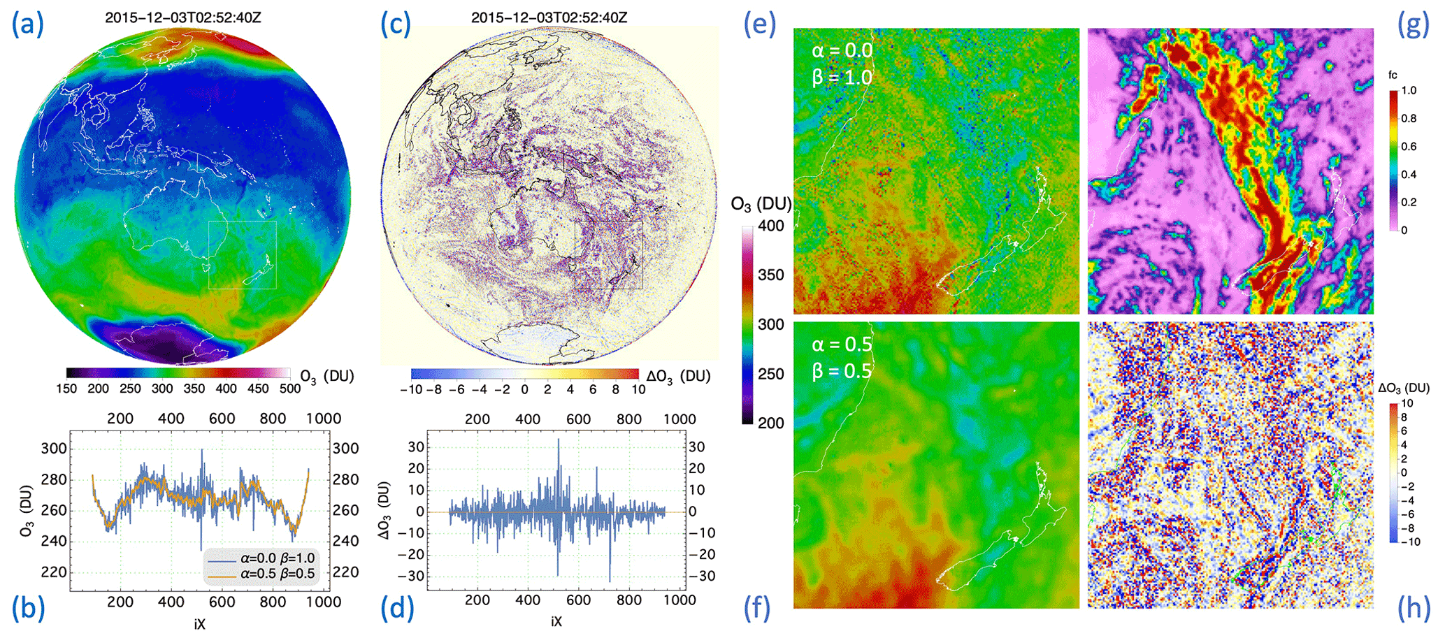
Figure 14 Retrieved O₃ from EPIC measurements of bands B1, B3, and B4 on 3 December 2015. (a) Optimized (i.e., $\mathit{\alpha }=\mathrm{0.5},\mathit{\beta }=\mathrm{0.5}$) O₃ map based on the SOE method; (b) a comparison of optimized (orange) and independent-pixel (blue, $\mathit{\alpha }=\mathrm{0},\mathit{\beta }=\mathrm{1}$) O₃ along the horizontal line (left to right) across the middle of the O₃ map in (a); (c) the O₃ difference map: $\mathrm{\Delta }{\mathrm{O}}_{\mathrm{3}}={\mathrm{O}}_{\mathrm{3}}\left(\mathrm{optimized}\right)-{\mathrm{O}}_{\mathrm{3}}\left(\mathrm{independent}\mathrm{pixel}\right)$; (d) the O₃ difference along the horizontal line across the middle of the map in (c); (e) a zoom-in of the independent-pixel O₃ map; (f) the optimized O₃ corresponding to the rectangle in (a); (g) cloud fraction f_c corresponding to (e) and (f); (h) O₃ difference (optimized − independent pixel), with a zoom-in corresponding to the rectangle in (c).

In summary, the SOE method performs single-band (B1 or B2) multiple-IFOV (or image-based) retrieval, yielding reflectivity (R) and total O₃ column (Ω), with the associated profile determined by the O₃ model (Eq. 12) that retains only the column-dependent M2TCO3 climatological profile X_m. The a priori knowledge of the O₃ distribution, which is spatially smooth, provides the extra information to correct the initial reflectivity estimation extrapolated from the characterization based on the longer wavelength bands.

5.2 Total O₃ column

Radiance measurements of EPIC B1 and B2 radiances have O₃ profile sensitivity, which is higher at B1 than at B2, especially at high zenith (SZA, VZA, or both) angles (as illustrated in Fig. 3). Compared to the measurement of a single O₃-sensitive band, both bands jointly provide more information that allows the refinement of climatological representation of the O₃ profile. This refinement is performed by adjusting the climatological profile with the most probable modal profile (e₁, see Eq. 12) so that both B1 and B2 yield the same total O₃ column.

For retrieval from EPIC, the full state vector to be inverted is $\mathit{x}=\mathit{\{}{\mathrm{\Omega }}_{\mathrm{0}},{\mathit{\gamma }}_{\mathrm{1}},\mathrm{\Xi },R_{\mathrm{1}},R_{\mathrm{2}}\mathit{\}}$, where Ω₀ is the total O₃ column, γ₁ the O₃ profile adjustment factor, Ξ the total vertical SO₂ column, and R₁ and R₂ the MLER parameters at EPIC B1 and B2. The regulated direct fitting of EPIC B1 and B2 radiances is applied to obtain retrieved full state vector x .

For each IFOV of EPIC, the O₃ vertical column is estimated first assuming there is no SO₂. The iteration starts with an initial state vector ${\mathit{x}}_{\mathrm{0}}=\mathit{\{}{\mathrm{\Omega }}_{\mathrm{0}}={\mathrm{\Omega }}_{\mathrm{c}},{\mathit{\gamma }}_{\mathrm{1}}=\mathrm{0},\mathrm{\Xi }=\mathrm{0},R_{\mathrm{1}}=R_{\mathrm{1}}^S,R_{\mathrm{2}}=R_{\mathrm{2}}^S\mathit{\}}$, where Ω_c is the climatological total column selected from the M2TCO3 climatology based on time and location. $R_{\mathrm{1}}^S$ and $R_{\mathrm{2}}^S$ are the corrected MLER parameters at B1 and B2, respectively, using the SOE method (see Sect. 5.1).

Since EPIC radiance measurement errors between any two bands are not correlated, the measurement error covariance matrix is diagonal: ${\mathbf{S}}_{\mathit{ϵ}}=\mathrm{diag}({\mathit{\sigma }}_{\mathrm{B}\mathrm{1}}^{\mathrm{2}}={\mathrm{0.00345}}^{\mathrm{2}},{\mathit{\sigma }}_{\mathrm{B}\mathrm{2}}^{\mathrm{2}}={\mathrm{0.00345}}^{\mathrm{2}})$, as estimated from the random errors of the radiance (I_M) measurements (see Sect. 6.2).

There is no correlation among retrieval parameters: total O₃ column (Ω₀), the deviation (ω₁) of the O₃ profile from the mean, SO₂ column (Ξ), and the MLER parameters R, except between R₁ and R₂. The diagonal elements of the a priori covariance matrix are ${\mathbf{S}}_{\mathrm{a}}=\mathrm{diag}({\mathit{\epsilon }}_{{\mathrm{\Omega }}_{\mathrm{0}}}^{\mathrm{2}}={\mathrm{10}}^{\mathrm{2}}$ DU², ${\mathit{\epsilon }}_{{\mathit{\gamma }}_{\mathrm{1}}}^{\mathrm{2}}={\mathrm{2}}^{\mathrm{2}}$ DU², ${\mathit{\epsilon }}_{\mathrm{\Xi }}^{\mathrm{2}}={\mathrm{0.0001}}^{\mathrm{2}}$ DU², ${\mathit{\epsilon }}_{R\mathrm{1}}^{\mathrm{2}}={\mathrm{0.001}}^{\mathrm{2}}$, ${\mathit{\epsilon }}_{R\mathrm{2}}^{\mathrm{2}}={\mathrm{0.001}}^{\mathrm{2}}$). The off-diagonal elements are equal to zero, $\mathit{\left\{}{S}_{\mathrm{a}}\right(i,j)=\mathrm{0}$, when i≠j}, except for the elements associated with R₁ and R₂, which may be set at $S_{\mathrm{a}}(\mathrm{4},\mathrm{5})=S_{\mathrm{a}}(\mathrm{5},\mathrm{4})=\mathrm{0.98}{\mathit{\epsilon }}_{R\mathrm{1}}{\mathit{\epsilon }}_{R\mathrm{2}}={\mathrm{0.0099}}^{\mathrm{2}}$, representing a high degree of correlation (0.99) between R₁ and R₂. This S_a essentially limits the adjustments at each iteration: $\left|\mathrm{\Delta }{\mathrm{\Omega }}_{\mathrm{0}}\right|\lesssim {\mathit{\epsilon }}_{{\mathrm{\Omega }}_{\mathrm{0}}}(\mathrm{10}$ DU), $\left|\mathrm{\Delta }{\mathit{\omega }}_{\mathrm{1}}\right|\lesssim {\mathit{\epsilon }}_{{\mathit{\gamma }}_{\mathrm{1}}}(\mathrm{2}$ DU), $\left|\mathrm{\Delta }\mathrm{\Xi }\right|\lesssim {\mathit{\epsilon }}_{\mathrm{\Xi }}({\mathrm{10}}^{-\mathrm{4}}$ DU), $\left|\mathrm{\Delta }{R}_{\mathrm{1}}\right|\lesssim {\mathit{\epsilon }}_{R\mathrm{1}}\left(\mathrm{0.001}\right)$, and $\left|\mathrm{\Delta }{R}_{\mathrm{2}}\right|\lesssim {\mathit{\epsilon }}_{R\mathrm{2}}\left(\mathrm{0.001}\right)$. The strong constraint on SO₂ ensures that its column Ξ never deviates far (>0.01 DU) from its initial value of 0 during the iteration, essentially enforcing an SO₂-free retrieval. The strong constraints on R₁ and R₂ also ensure that they remain nearly the same as their initial values $R_{\mathrm{1}}^S$ and $R_{\mathrm{2}}^S$. The constraints on O₃ parameters are quite loose. Especially towards the convergence of the iteration, the absolute adjustment of each component is much smaller than the corresponding standard deviation, i.e., the square root of the corresponding diagonal element of S_a.

With the setup of error and a priori covariance matrices S_ϵ and S_a, the initial state vector x₀ is updated (Eq. 17) iteratively using Δx from Eq. 25 until the exit of the iteration when $\left|\mathrm{\Delta }{\mathrm{\Omega }}_{\mathrm{0}}\right|<\mathrm{0.5}$ DU and $\left|\mathrm{\Delta }{\mathit{\gamma }}_{\mathrm{1}}\right|<\mathrm{0.5}$ DU. The retrieved total O₃ column (Ω) is obtained by integrating the profile $\mathbf{X}={\mathbf{X}}_{\mathrm{m}}\left({\mathrm{\Omega }}_{\mathrm{0}}\right)+{\mathit{\gamma }}_{\mathrm{1}}{e}_{\mathrm{1}}\left({\mathrm{\Omega }}_{\mathrm{0}}\right)$. In processing EPIC data, the initial O₃ column Ω_c of x₀ for an IFOV may be set to the column Ω of a previous (or nearby) IFOV to improve the speed of convergence of the iteration.

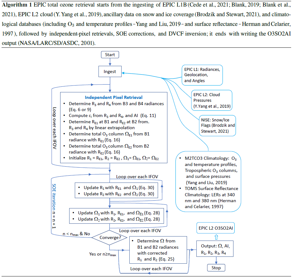
Here we list the algorithmic procedure (see the flowchart in Algorithm 1), titled EPIC total ozone retrieval, that is applied to each EPIC level-1b (L1B) granule, which contains spectral measurements, as well as geolocation and angular information for all the IFOVs of a snapshot of the sunlit side of the Earth, to produce the level-2 (L2) O3SO2AI product. The contents of a sample O3SO2AI granule are displayed in Fig. 15, including total O₃, LER, and AI, which are respectively shown in Fig. 15c, e, and f. For comparison, the MERRA-2 assimilated O₃ total columns, interpolated to the time and location of EPIC IFOVs, are included in Fig. 15d, their differences O₃(EPIC)−O₃(MERRA-2) in Fig. 15g, and the histogram in Fig. 15h. This comparison reveals excellent agreement between MERRA-2 and EPIC total O₃, showing nearly identical O₃ spatial distributions with similar highs and lows. Quantitatively, the differences for samples with VZA $\le \mathrm{70}{}^{\circ }$ are characterized by a low mean offset ($\mathit{\mu }\left(\mathrm{EPIC}\right)=-\mathrm{0.2}$ %) and a narrow spread (standard deviation σ(EPIC)=2.52 %). Figure 15 includes the intermediate results of the EPIC total O₃ processing (see the procedure in Algorithm 1), showing the total O₃ columns retrieved from B1 in panel (a) and from B2 in panel (b) using the SOE method. Both B1 and B2 total columns closely resemble the MERRA-2 (panel d) and EPIC (panel c) total O₃ fields, with difference statistics showing slightly worse offsets (μ(EPIC B1)=0.25 % and $\mathit{\mu }\left(\mathrm{EPIC}\mathrm{B}\mathrm{2}\right)=-\mathrm{0.41}$ %) and higher standard deviations (σ(EPIC B1)=2.68 % and σ(EPIC B2)=2.68 %). The improved agreement with MERRA-2 is significant, reducing the B1 O₃ spread by $\sqrt{{\mathit{\sigma }}^{\mathrm{2}}\left(\mathrm{EPIC}\mathrm{B}\mathrm{1}\right)-{\mathit{\sigma }}^{\mathrm{2}}\left(\mathrm{EPIC}\right)}=\mathrm{0.9}$ % (or 2.8 DU) and the B2 O₃ spread by a similar amount. These better agreements are consistent over time and location, substantiating the improved retrieval with both O₃-sensitive bands over a single one, which is adopted by the TOMS-V8 algorithm. Since the MERRA-2 O₃ field from the assimilation of independent measurements of the Aura OMI and Aura Microwave Limb Sounder (MLS) provides highly realistic spatiotemporal O₃ representation, the smaller spread between the two-band (B1 and B2) EPIC and MERRA-2 total O₃ columns indicates that the inclusion of more O₃-sensitive bands enables more accurate retrievals.

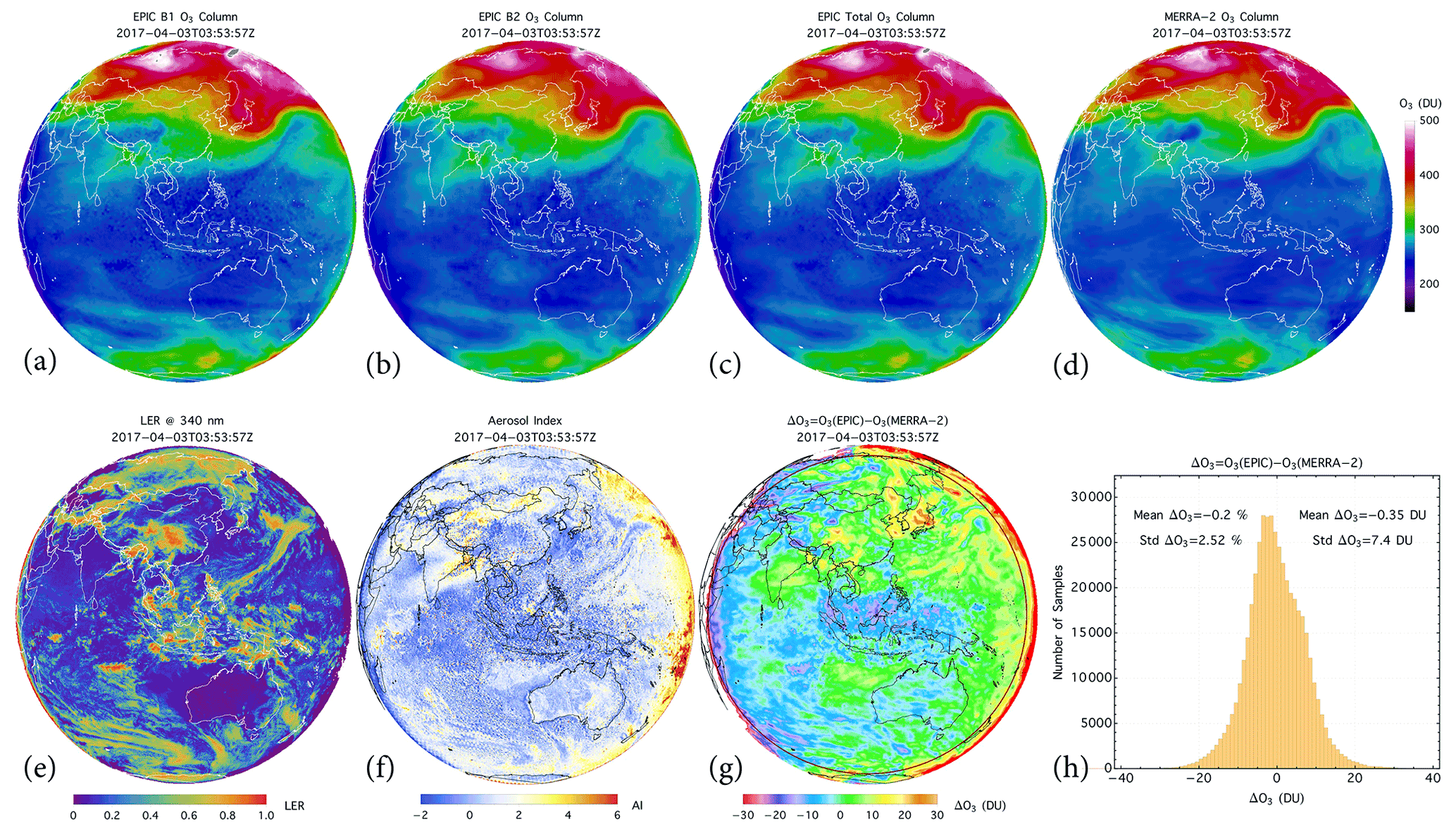
Figure 15 An L2 O3SO2AI granule contains the total O₃ vertical columns (c), LER at 340 nm (e), and AI (f) retrieved from EPIC UV measurements at 03:53:57 UTC on 3 April 2017. (a) Total O₃ column (referred to as B1 total O₃ column) retrieved from EPIC B1, B3, and B4. (b) Total O₃ column (referred to as B2 total O₃ column) retrieved from EPIC B2, B3, and B4. (c) Total O₃ from all four bands. (d) Coincident MERRA-2 total O₃ columns. (g) The total O₃ difference: O₃(EPIC)−O₃(MERRA-2). (h) The histogram of the O₃ differences with SZA $\le \mathrm{70}{}^{\circ }$, i.e., samples within the circle in (g), with a mean difference $\mathit{\mu }\left(\mathrm{EPIC}\right)=-\mathrm{0.20}$ % (or −0.35 DU) and a standard deviation σ(EPIC)=2.52 % (or 7.4 DU). Similarly, the O₃ difference, O₃(EPIC B1)−O₃(MERRA-2), has a mean of μ(EPIC B1)=0.25 % (or 1.03 DU) and a standard deviation σ(EPIC B1)=2.68 % (or 7.9 DU), and O₃(EPIC B2)−O₃(MERRA-2) has a mean $\mathit{\mu }\left(\mathrm{EPIC}\mathrm{B}\mathrm{2}\right)=-\mathrm{0.41}$ % (or −1.08 DU) and a standard deviation σ(EPIC B2)=2.68 % (or 7.8 DU).

5.3 Volcanic SO₂

EPIC B1 and B2 radiances respond to both O₃ and SO₂ absorptions, but with very different (see Fig. 13) sensitivities: SO₂ is more than twice as UV-absorbent as O₃ at B1; in contrast, it is significantly less at B2 and about 70 % as absorbent as O₃. Consequently, the estimate of O₃ absorption signals at these two bands would result in an error due to the presence of SO₂ in the atmosphere: 1 DU of SO₂ would usually yield more than 2 DU O₃ error at B1, but only about 0.7 DU error at B2. This big difference in absorption sensitivities facilitates the detection of SO₂ in the atmosphere. Given a radiance signal-to-noise ratio (SNR) of 290:1, the theoretical minimum detectable level of SO₂ enhancement is ∼0.5 DU in the upper troposphere and above. However, it is difficult to distinguish SO₂ at this minimum level from other changes, such as the O₃ profile or surface spectral reflectance, since they can induce similar changes in the measured radiances. This difficulty is increased by EPIC's asynchronous spectral measurements, which may yield spectral variation similar to the response to adding SO₂ in the atmosphere. Consequently, low levels of SO₂ elevation cannot be reliably detected in EPIC observations. For significant SO₂ elevations, typically those from volcanic eruptions, B1 O₃ is much higher than B2 O₃ (i.e., Ω₁>Ω₂) from the total O₃ retrieval (described in Sect. 5.2). Adjusting the O₃ profile shape or changing the spectral reflectance of the underlying surface usually cannot eliminate this large O₃ discrepancy between the two bands. Therefore, a high positive value of ΔΩ can be used to flag the presence of SO₂. Furthermore, a volcanic plume usually occupies a contiguous area with a limited spatial extent. Thus, ΔΩ and Ω₁ enhancements resulting from volcanic SO₂ plume occur over a large group of connected IFOVs instead of isolated or a small group of disconnected IFOVs. Based on these characteristics of volcanic SO₂ plumes, we next describe an algorithmic procedure to flag IFOVs with SO₂ enhancements.

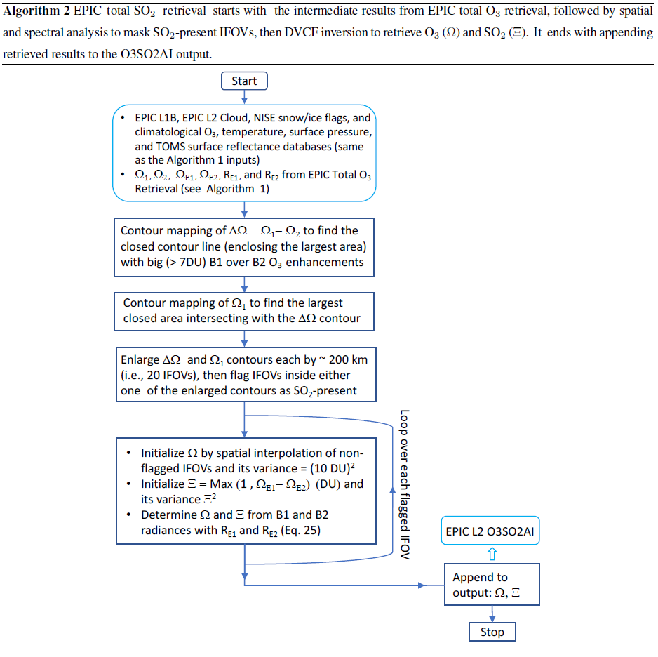
For reliable SO₂ detection, the following procedure is applied to identify the presence of SO₂ in an IFOV. First, IFOVs of likely SO₂ elevations are flagged through spatial analysis of the differential O₃ field (i.e., $\mathrm{\Delta }\mathrm{\Omega }={\mathrm{\Omega }}_{\mathrm{1}}-{\mathrm{\Omega }}_{\mathrm{2}}$, EPIC B1 and B2 O₃ difference), accomplished through contour mapping to find closed areas of local ΔΩ enhancements, i.e., areas within closed contours with Ω₁ considerably higher (≥7 DU) than the Ω₂ values (see, e.g., Fig. 16b). The IFOVs within this ΔΩ contour likely have SO₂ elevation around 5 DU or above. Next, contour mapping of Ω₁ is performed to find the longest closed contour line in the area that extends 150 pixels off the extrema of the ΔΩ contour (i.e., an image rectangle with a minimum of 300×300 IFOVs or 3000×3000 km² that covers the ΔΩ contour). Within this closed Ω₁ contour, IFOVs with likely SO₂ enhancements are flagged when Ω₁>Ω₂. This flagging is then extended to the adjacent areas outside the two contours to identify IFOVs with possible SO₂ contamination. For most volcanic plumes, these two contours overlap each other greatly. Including areas within the Ω₁ contour and the adjacent outside regions is designed to capture plumes with lower SO₂ elevations.

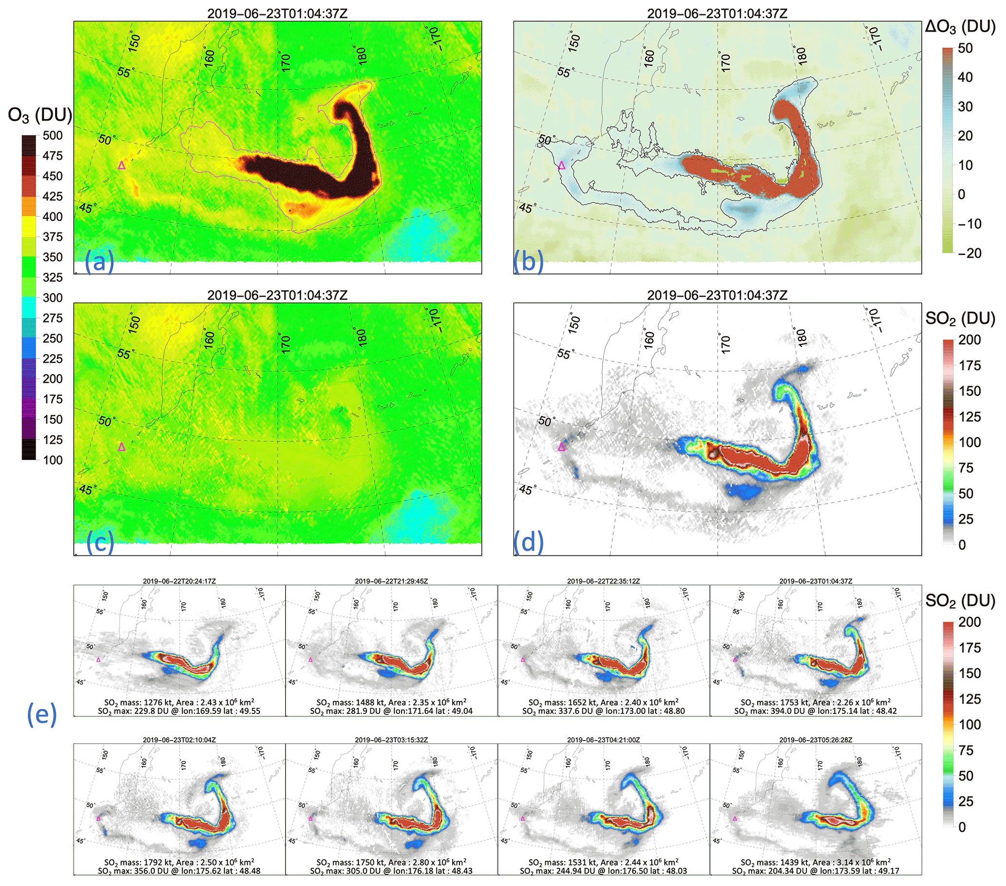
Figure 16 EPIC observation of the volcanic plume on 23 June 2019 from the previous day's eruption of Raikoke volcano (represented by Δ in each panel) in the central Kuril Islands of Russia. (a) B1 O₃ column (Ω₁) from EPIC total ozone retrieval and the elevated O₃ contour. (b) B1 and B2 O₃ column difference ($\mathrm{\Delta }\mathrm{\Omega }={\mathrm{\Omega }}_{\mathrm{1}}-{\mathrm{\Omega }}_{\mathrm{2}}$) and elevated ΔΩ contour. (c) Vertical O₃ column from EPIC total SO₂ retrieval (see Algorithm 2). (d) Vertical SO₂ column from EPIC total SO₂ retrieval. (e) SO₂ vertical column retrieved from a series of eight consecutive EPIC observations of the Raikoke plume, represented by a 1.5 km thick GDF layer centered at an altitude of 13 km above sea level.

Once detected, the SO₂ quantification follows the DVCF retrieval with the initial state and a priori covariance setting described next. For the IFOV identified with SO₂ contamination, the initial O₃ values are spatially interpolated from the background Ω₁ field, γ₁=0, and initial SO₂ column ${\mathrm{\Xi }}_{\mathrm{0}}={\mathrm{\Omega }}_{\mathrm{1}}-{\mathrm{\Omega }}_{\mathrm{2}}$, integrated from a vertical profile specified by a generalized distribution function (GDF; Yang et al., 2010) with a width and a center altitude appropriate for the plume. The corresponding elements of the a priori covariance matrix are ${\mathbf{S}}_{\mathrm{a}}=\mathrm{diag}({\mathit{\epsilon }}_{{\mathrm{\Omega }}_{\mathrm{0}}}^{\mathrm{2}}={\mathrm{10}}^{\mathrm{2}}$ DU², ${\mathit{\epsilon }}_{{\mathit{\gamma }}_{\mathrm{1}}}^{\mathrm{2}}={\mathrm{2}}^{\mathrm{2}}$ DU², ${\mathit{\epsilon }}_{\mathrm{\Xi }}^{\mathrm{2}}={{\mathrm{\Xi }}_{\mathrm{0}}}^{\mathrm{2}}$ DU²), i.e., the variances associated with O₃ are the same as those for total O₃ retrieval, while the SO₂ column variance is equal to the square of the initial SO₂ estimate (Ξ₀), which is a weak constraint to allow Ξ to change freely responding to the measurement. Other retrieval settings are kept the same as in the total O₃ retrieval described in the previous section. We list the complete algorithmic procedure in Algorithm 2, titled EPIC total SO₂ retrieval, for SO₂ detection and quantification from EPIC UV observations.

The algorithmic procedure (listed in Algorithm 2) applies to regions where EPIC observes volcanic plumes to produce the EPIC volcanic SO₂ product. Figure 16 illustrates the detection and quantification of volcanic SO₂ from EPIC observations. Spatial analyses (i.e., contour mappings) of the intermediate results (Fig. 16a and b) of the total O₃ processing (see Algorithm 1) provide reliable detection of SO₂ elevations. The SO₂-flagged IFOVs are then processed with the DVCF algorithm to retrieve total vertical O₃ and SO₂ columns simultaneously, with results shown in Fig. 16c and d, respectively. Comparison of the two O₃ fields in Fig. 16 shows that the initial O₃ elevations (Fig. 16a) due to the presence of SO₂ are nearly entirely removed in the final O₃ field (Fig. 16c), demonstrating that the combined retrieval of O₃ and SO₂ achieves consistent O₃ values inside and outside the plumes. The achieved internal consistency indirectly validates the SO₂ columns. In Fig. 16e, we show maps of DVCF-retrieved SO₂ columns from a series of eight consecutive EPIC observations of the Raikoke plume in Fig. 16e, with the maximum SO₂ value, the total SO₂ mass, and the total area covered by elevated SO₂ displayed in each snapshot. These results illustrate the high-cadence observing capability and high-quality SO₂ measurements of EPIC.

6 Error analysis

We describe in this section how algorithm physics treatments and various sources contribute to the retrieval uncertainties and provide error estimates of the EPIC O₃ and SO₂ products.

6.1 General expression

The spectral measurements, represented by a column vector y of length m (the number of wavelength bands), are written explicitly with all the dependent parameters and possible errors and then expanded with respect to the linearization point (x_L):

$$\begin{array}{}\text{(31)}& \mathit{y}=\ln {\mathbf{I}}_m=\ln {\mathbf{I}}_{\mathrm{TOA}}(\mathit{\omega },\mathit{\xi },\mathit{b})+{\mathit{ϵ}}_{\mathrm{m}}\end{array}$$

$$\begin{array}{}\text{(32)}& \begin{array}{rl}=& \ln {\mathbf{I}}_{\mathrm{TOA}}({\mathit{\omega }}_{\mathrm{L}},{\mathit{\xi }}_{\mathrm{L}},{\mathit{b}}_{\mathrm{L}})+{\mathbf{k}}_{\mathit{\omega }}(\mathit{\omega }-{\mathit{\omega }}_{\mathrm{L}})\\ & +{\mathbf{k}}_{\mathit{\xi }}(\mathit{\xi }-{\mathit{\xi }}_{\mathrm{L}})+{\mathbf{k}}_b(\mathbf{b}-{\mathbf{b}}_{\mathrm{L}})+{\mathit{ϵ}}_{\mathrm{f}}+{\mathit{ϵ}}_{\mathrm{m}},\end{array}\end{array}$$

where the column vectors of length n_l (the number of atmospheric layers), ω, and ξ respectively represent the actual vertical profiles for O₃ and SO₂, while ω_L is the climatological O₃ profile equal to X_m(Ω_L)+γ₁e₁(Ω_L) and ξ_L the prescribed SO₂ profile specified by a GDF layer with an integrated vertical column equal to Ξ_L. The profile weighting functions, ${\mathbf{k}}_{\mathit{\omega }}=\frac{-\partial \ln {\mathbf{I}}_{\mathrm{TOA}}}{\partial \mathit{\omega }}{|}_{\mathit{\omega }={\mathit{\omega }}_{\mathrm{L}}}$ and ${\mathbf{k}}_{\mathit{\xi }}=\frac{-\partial \ln {\mathbf{I}}_{\mathrm{TOA}}}{\partial \mathit{\xi }}{|}_{\mathit{\xi }={\mathit{\xi }}_{\mathrm{L}}}$, are m×n_l matrices, with each of the rows equal to the product of absorber cross-sections at one spectral band and the layer AMFs (i.e., the mean photon path lengths through the atmospheric layers). Likewise, b and b_L are respectively a set of the exact forward model parameters and those used in the linearization, with the corresponding sensitivity matrix ${\mathbf{k}}_b=\frac{-\partial \ln {\mathbf{I}}_{\mathrm{TOA}}}{\partial \mathit{b}}{|}_{\mathit{b}={\mathit{b}}_{\mathrm{L}}}$. These forward model parameters may include the spectral-dependent MLER parameters, the ground surface and the OCP cloud pressures, the atmospheric temperature profile, the absorption cross-sections of O₃ and SO₂, and the parameters that specify the ISRFs of the spectral bands. The column vector ϵ_f is the forward modeling errors of the spectral bands, such as the approximate radiative transfer through Earth's spherical atmosphere and the incomplete accounting for RRS contributions. The last term ϵ_m is a column vector representing the spectral radiance errors of the instrument, including random noises and radiometric calibration biases.

Using the definition $\mathrm{\Delta }\mathit{x}=\mathit{x}-{\mathit{x}}_{\mathrm{L}}$ and putting Eq. (32) into residual Δy_L, Eq. (25) is rewritten as

$$\begin{array}{}\text{(33)}& {\displaystyle }\begin{array}{rl}\mathit{x}-{\mathit{x}}_{\mathrm{L}}& =\mathbf{G}\left[{\mathbf{k}}_{\mathit{\omega }}\left(\mathit{\omega }-{\mathit{\omega }}_{\mathrm{L}}\right)+{\mathbf{k}}_{\mathit{\xi }}\left(\mathit{\xi }-{\mathit{\xi }}_{\mathrm{L}}\right)+{\mathbf{k}}_{\mathrm{b}}\left(\mathit{b}-{\mathit{b}}_{\mathrm{L}}\right)\right.\\ & \left.+{\mathit{ϵ}}_{\mathrm{f}}+{\mathit{ϵ}}_{\mathrm{m}}\right]\end{array}\text{(34)}& {\displaystyle }\begin{array}{rl}& ={\mathbf{A}}_{\mathit{\omega }}\left(\mathit{\omega }-{\mathit{\omega }}_{\mathrm{L}}\right)+{\mathbf{A}}_{\mathit{\xi }}\left(\mathit{\xi }-{\mathit{\xi }}_{\mathrm{L}}\right)+{\mathbf{Gk}}_{\mathrm{b}}\left(\mathit{b}-{\mathit{b}}_{\mathrm{L}}\right)\\ & +\mathbf{G}{\mathit{ϵ}}_{\mathrm{f}}+\mathbf{G}{\mathit{ϵ}}_{\mathrm{m}},\end{array}\end{array}$$

where A_ω=Gk_ω and A_ξ=Gk_ξ are the averaging kernels (AKs) for O₃ and SO₂, respectively. Equation (34) describes how various error sources, from mismatches in absorber profiles to errors in model and measurement, propagate into the final result (x). The rows associated with the O₃ and SO₂ columns can be extracted from the vector equation (Eq. 34) and written as

$$\begin{array}{}\text{(35)}& {\displaystyle }\mathrm{\Omega }-{\mathrm{\Omega }}_{\mathrm{T}}=\left({\mathbf{A}}_{\mathrm{\Omega }}-\mathrm{1}\right)\left(\mathit{\omega }-{\mathit{\omega }}_{\mathrm{L}}\right)+{\mathbf{G}}_{\mathrm{\Omega }}{\mathit{ϵ}}_{\mathrm{\Omega }},\text{(36)}& {\displaystyle }\mathrm{\Xi }-{\mathrm{\Xi }}_{\mathrm{T}}=\left({\mathbf{A}}_{\mathrm{\Xi }}-\mathrm{1}\right)\left(\mathit{\xi }-{\mathit{\xi }}_{\mathrm{L}}\right)+{\mathbf{G}}_{\mathrm{\Xi }}{\mathit{ϵ}}_{\mathrm{\Xi }},\end{array}$$

after subtracting Ω_T−Ω_L and Ξ_T−Ξ_L from the row equations, respectively. Here Ω_T and Ξ_T are the true O₃ and SO₂ columns, integrated from the corresponding true O₃ (ω) and SO₂ (ξ) profiles. A_Ω and G_Ω are the row vectors associated with the retrieved O₃ column Ω from the corresponding matrices A_ω and G. Analogously, A_Ξ and G_Ξ are the row vectors related to the retrieved SO₂ column Ξ taken from the matrices A_ξ and G, respectively. The constant row vector 1 contains the value 1 for all its elements. Thus, its dot product with a vertical profile (a column vector) is equivalent to the summation of all the individual layer amounts, yielding the total column. The column vector ϵ_Ω represents the total error combined from various sources impacting the total O₃ accuracy, including errors in model parameters k_b(b−b_L), forward modeling ϵ_f, spectral measurements ϵ_m, and the other absorber k_ξ(ξ−ξ_L). Similarly, ϵ_Ξ represents the combined total error affecting total SO₂ accuracy with the other absorber term being replaced by k_ω(ω−ω_L).

Retrieval errors can be characterized using Eqs. (35) and (36), provided errors from various sources are sufficiently small that forward modeling responds linearly to these deviations. However, substantial retrieval errors usually result from simplified physics treatments, which constrain the forward model to be radiative transfer in a molecular atmosphere over Lambertian surfaces. These errors may be called the AMF errors because the simplified physics treatments cannot, in general, reproduce the paths of photons through the observed atmosphere, even though they enable radiance matching between measurement and modeling. The deviations of mean paths lead to retrieval errors in O₃ and SO₂ because the interpretation of measured radiance through radiance matching requires accurate modeling of mean photon paths (i.e., the AMFs). The retrieval errors from the simplified physics treatment can be estimated using closed-loop tests (i.e., realistic forward modelings and then inverse retrieval with simplified physics treatments). Next, we provide uncertainty estimates of O₃ and SO₂ retrievals contributed from various error sources and simplified physics treatments.

6.2 Uncertainty estimates

6.2.1 Measurement errors

Errors in EPIC spectral measurements contribute to uncertainties in retrieved O₃ and SO₂ columns (Ω and Ξ). Taking the terms associated with radiance errors from Eqs. (35) and (36), retrieval errors are written as

$$\begin{array}{}\text{(37)}& {\displaystyle }\mathrm{\Delta }\mathrm{\Omega }={\mathbf{G}}_{\mathrm{\Omega }}\left({\mathit{ϵ}}_{\mathrm{m}}+{\mathbf{k}}_R\mathrm{\Delta }\mathbf{R}\right),\text{(38)}& {\displaystyle }\mathrm{\Delta }\mathrm{\Xi }={\mathbf{G}}_{\mathrm{\Xi }}({\mathit{ϵ}}_{\mathrm{m}}+{\mathbf{k}}_R\mathrm{\Delta }\mathbf{R}).\end{array}$$

These equations specify how measurement errors (ϵ_m) of the O₃-sensitive bands and the MLER parameter errors (ΔR) due to the measurement errors in the weak absorption bands propagate into retrieved vertical columns.

Biases in radiance measurements lead to systematic errors in retrieved vertical columns. While the actual radiance biases are unknown, they are likely less than 1 % for EPIC UV bands. For radiance biases within ±1 %, the systematic O₃ and SO₂ column errors are within $\pm \sim \mathrm{15}$ and $\pm \sim \mathrm{8}$ DU, respectively, as estimated from Eqs. (37) and (38). These retrieval column errors are primarily controlled by the relative differences of spectral errors without significant dependence on the column amounts or surface reflectance. The retrieval biases vary with observing conditions given the same percentage radiance errors due to gain matrices (G_Ω and G_Ξ) significantly depending on viewing and illumination angles.

In addition to systematic errors, radiance measurement noises add random errors to the retrieved columns. Retrieval errors due to random radiance noises (specified with normal distributions) are unbiased, with mean values, μ(ΔΩ) and μ(ΔΞ), close to zero and standard deviations, σ(ΔΩ) and σ(ΔΞ), proportional to standard deviations of radiance noises. The signal-to-noise ratios for EPIC UV bands are 290:1 (Herman et al., 2018), equivalent to a noise level (standard deviation) of 0.345 % $(\mathrm{1}/\mathrm{290})$. This level is consistent with high-frequency radiance fluctuations (with standard deviations equal to 0.373 %, 0.354 %, 0.354 %, and 0.368 % for B1 to B4, respectively) within cloud-free scenes observed by EPIC. With a setting of equal standard deviations for the four UV bands (i.e., ${\mathit{ϵ}}_{\mathrm{m}}=\mathit{\{}\mathrm{0.345}\mathit{\%},\mathrm{0.345}\mathit{\%},\mathrm{0.345}\mathit{\%},\mathrm{0.345}\mathit{\%}\mathit{\}}$), the estimated column O₃ noise level is σ(ΔΩ)≃3.2 DU at low viewing zenith angles, decreases gradually with higher zenith angles, reaches a minimum of ∼1.5 DU at $\sim \mathrm{75}{}^{\circ }$, and then rebounds quickly with further increases in zenith angles (see Fig. 17). The noise level of SO₂ columns, σ(ΔΞ), exhibits a similar angular dependence as shown in Fig. 17, primarily following the angular variation of the gain matrix G_Ξ. These angular-dependent column noises are insensitive to the column amounts or the surface reflectance.

Figure 17 Noise levels, i.e., standard deviations (σ) of O₃ and SO₂ errors (Δ), contributed from the random noises in EPIC spectral measurements. The SO₂ noise estimate is for a layer at an altitude 11 km above sea level.

6.2.2 Model parameter errors

Retrieval errors due to uncertainties in model parameters, including molecular absorption cross-sections (σ) and atmospheric temperature profiles (T), are estimated as

$$\begin{array}{}\text{(39)}& {\displaystyle }\mathrm{\Delta }\mathrm{\Omega }={\mathbf{G}}_{\mathrm{\Omega }}\left(\left({\mathbf{m}}_z\mathrm{\Delta }{\mathit{\sigma }}_{{\mathrm{O}}_{\mathrm{3}}}\right)\mathit{\omega }+\left({\mathbf{m}}_z{\displaystyle \frac{\partial {\mathit{\sigma }}_{{\mathrm{O}}_{\mathrm{3}}}}{\partial \mathbf{T}}}\right)\left(\mathit{\omega }\mathrm{\Delta }\mathbf{T}\right)\right),\text{(40)}& {\displaystyle }\mathrm{\Delta }\mathrm{\Xi }={\mathbf{G}}_{\mathrm{\Xi }}\left(\left({\mathbf{m}}_z\mathrm{\Delta }{\mathit{\sigma }}_{{\mathrm{SO}}_{\mathrm{2}}}\right)\mathit{\xi }+\left({\mathbf{m}}_z{\displaystyle \frac{\partial {\mathit{\sigma }}_{{\mathrm{SO}}_{\mathrm{2}}}}{\partial \mathbf{T}}}\right)\left(\mathit{\xi }\mathrm{\Delta }\mathbf{T}\right)\right),\end{array}$$

where $\left({\mathbf{m}}_z\mathrm{\Delta }{\mathit{\sigma }}_{{\mathrm{O}}_{\mathrm{3}},{\mathrm{SO}}_{\mathrm{2}}}\right)$ and $\left({\mathbf{m}}_z\frac{\partial {\mathit{\sigma }}_{{\mathrm{O}}_{\mathrm{3}},{\mathrm{SO}}_{\mathrm{2}}}}{\partial \mathbf{T}}\right)$ are m×n_l matrices with elements $\mathit{\left\{}{m}_{z_j}\right({\mathit{\lambda }}_i\left)\mathrm{\Delta }{\mathit{\sigma }}_{{\mathrm{O}}_{\mathrm{3}},{\mathrm{SO}}_{\mathrm{2}}}\right({\mathit{\lambda }}_i,T_j),i=\mathrm{1}\mathrm{\dots }m,j=\mathrm{1}\mathrm{\dots }{n}_{\mathrm{l}}\mathit{\}}$ and $\mathit{\left\{}{m}_{z_j}\right({\mathit{\lambda }}_i)\frac{\partial {\mathit{\sigma }}_{{\mathrm{O}}_{\mathrm{3}},{\mathrm{SO}}_{\mathrm{2}}}({\mathit{\lambda }}_i,T)}{\partial T}{|}_{T_j},i=\mathrm{1}\mathrm{\dots }m,j=\mathrm{1}\mathrm{\dots }{n}_{\mathrm{l}}\mathit{\}}$, respectively. Here m_z (see Eq. 7) is the mean photon path length through a layer at altitude z, $\mathrm{\Delta }{\mathit{\sigma }}_{{\mathrm{O}}_{\mathrm{3}},{\mathrm{SO}}_{\mathrm{2}}}$ represents errors in O₃ or SO₂ cross-sections, and ΔT represents errors in atmospheric temperature profiles.

The BDM O₃ cross-sections (Daumont et al., 1992; Brion et al., 1993; Malicet et al., 1995, commonly abbreviated as BDM) and the BW SO₂ cross-sections (Birk and Wagner, 2018) are used in O₃ and SO₂ retrievals from EPIC. These baseline cross-sections contain errors, which are not known quantitatively but can be estimated by comparing with alternative cross-sections. Specifically, the BW O₃ cross-sections (Birk and Wagner, 2021) and the SO₂ absorption cross-sections of Bogumil et al. (2003) are the alternatives that can replace the baselines for EPIC retrievals. The cross-section errors, $\mathrm{\Delta }{\mathit{\sigma }}_{{\mathrm{O}}_{\mathrm{3}}}$ in Eq. (39) and $\mathrm{\Delta }{\mathit{\sigma }}_{{\mathrm{SO}}_{\mathrm{2}}}$ in Eq. (40), are estimated based on the differences between the alternatives and baselines, showing that alternative O₃ and SO₂ cross-sections are slightly (about 0.1 % to 1.1 %) lower than the corresponding baselines at EPIC B1 and B2. These biases in cross-sections result in O₃ column biases between 0.5 % and 2 % as well as SO₂ column biases between 1 % and 2 % depending on the effective cross-section differences. The temperature dependence of the BW O₃ cross-sections behaves quite differently from the BDM (Bak et al., 2020), especially at EPIC B2, contributing to the high ends of O₃ biases (>1.0 %), which occur predominantly at high (viewing or solar) zenith angles when O₃ retrieval becomes more sensitive to EPIC B2 radiance.

Both O₃ and SO₂ cross-sections are significantly dependent on temperatures. Thus, accurate temperature profiles are needed to determine atmospheric absorption properties for modeling of measured radiances. As mentioned in Sect. 3, MERRA-2 climatological temperature profiles (Yang and Liu, 2019) are used for retrievals from EPIC. Actual temperature profiles differ from the climatological profiles. Over a short period (e.g., a day), the spatial distribution of these differences is not random, leading to retrieval errors that are unevenly distributed spatially. However, actual temperature profiles are normally distributed around the climatological mean over a long period (e.g., a month) for a location. Therefore, temperature profile mismatches add random components, which average to zero over a long time, to the total errors. The variances of these random errors are proportional to the layer-column-weighted temperature error variances. Estimated from the variances of temperature profiles (Yang and Liu, 2019), the random components, σ(ΔΩ), are ∼0.3 % in the tropics, increase to ∼0.7 % in the midlatitudes, and reach ∼1 % at high latitudes. Similarly, random errors, σ(ΔΞ), are ∼0.8 % in the tropics, ∼1.7 % in the midlatitudes, and ∼3.5 % at high latitudes.

6.2.3 Forward modeling errors

The MLER treatment adopted for the retrieval algorithm allows the use of the vector radiative transfer code, TOMRAD, as the forward model to simulate measured radiances and weighting functions. TOMRAD implements Dave's iterative solution (Dave, 1964) with pseudo-spherical approximation (Caudill et al., 1997) to the problem of the transfer of solar radiation through a molecular atmosphere over a Lambertian surface. The forward modeling with TOMRAD is accurate for EPIC observations around the center of its hemispheric view, with radiance errors (ϵ_f) of all EPIC UV bands less than ±0.2 % for VZA $<\mathrm{50}{}^{\circ }$. Note that for EPIC observations, each of its IFOVs has similar VZA and SZA (see Fig. 1) with differences $\mathrm{VZA}-\mathrm{SZA}<\pm \mathrm{9}{}^{\circ }$. As EPIC observations move towards the edge, the pseudo-spherical model atmosphere deviates more from Earth's spherical atmosphere in accounting for atmospheric attenuation and multiple scattering, resulting in more significant errors in modeled radiances, whose maximum errors increase to about ±1 % at 75^∘ VZA and about ±2 % at 85^∘ VZA (Caudill et al., 1997). RRS corrections are included in the forward modeling, and they are well within ±1 % for EPIC UV bands (see, e.g., Fig. 10). Incomplete RRS corrections are expected to add less than ±0.1 % to the forward modeling errors.

Unlike the calibration biases being insensitive to observing conditions and having no correlation among different bands, the forward modeling errors vary with absorber amounts and surface reflection, and they overestimate or underestimate similarly for all the UV bands depending on the viewing and illumination geometry. How these radiance errors propagate into the retrieved columns can be estimated using Eqs. (37) and (38), with error source terms replaced by ϵ_f and ΔR due to modeling errors in the long wavelength bands. With the radiance errors estimated above, these equations yield retrieval errors up to $\pm \sim \mathrm{0.6}$ and $\pm \sim \mathrm{0.3}$ DU when VZA $<\mathrm{50}{}^{\circ }$, increasing to $\pm \sim \mathrm{1.5}$ and $\pm \sim \mathrm{1}$ DU at VZA $=\mathrm{75}{}^{\circ }$, as well as $\pm \sim \mathrm{5}$ and $\pm \sim \mathrm{15}$ DU at VZA $=\mathrm{85}{}^{\circ }$, respectively, for O₃ and SO₂ vertical column errors. These are systematic errors and vary between high and low biases spatially depending on observing conditions, especially the viewing and illumination geometry.

6.2.4 Profile errors

As described in Sect. 3, a column-dependent O₃ profile, whose tropospheric integration matches the climatological tropospheric column, is used to specify the vertical distribution of a retrieved total O₃ column. This retrieved profile (ω_L), which represents the likely vertical distribution of the retrieved O₃ vertical column, invariably differs from the actual profile (ω). The O₃ error (ΔΩ) due to a profile errors (ω−ω_L) can be quantified using the first term on the rhs of Eq. (35), which is regulated by the retrieval AK (A_Ω). Examples of AKs for EPIC total O₃ retrievals are shown in Fig. 18a and c, illustrating how A_Ω changes with viewing geometry. For low VZAs ($<\mathrm{55}{}^{\circ }$), O₃ AKs are close to 1 above the upper troposphere, and therefore profile mismatches in this altitude region result in insignificant retrieval errors. However, profile mismatches produce sizable retrieval errors for high VZAs. In the troposphere, O₃ AKs change with surface reflectance in addition to angular dependence. Under cloud-free conditions, O₃ AKs drop quickly towards low-reflectivity surfaces, more so at high zenith angles (see, e.g., Fig. 18a). Above highly reflective surfaces (e.g., snow, ice, or bright clouds), O₃ AKs increase drastically (see Fig. 18c), indicating enhanced sensitivity to tropospheric profile, especially at low zenith angles. Evidently, O₃ errors due to profile mismatches primarily come from the troposphere for low zenith angles for both low- and high-reflectivity surfaces, though stratospheric contributions increase substantially with higher zenith angles, more significantly for a low-reflectivity surface. In general, errors due to the profile shape are reduced for high-reflectivity surfaces.

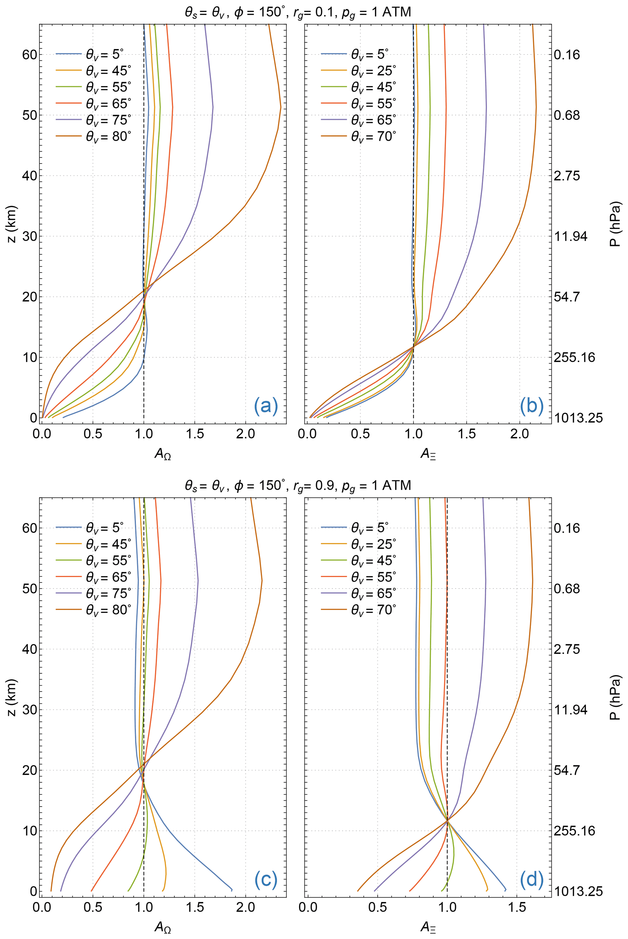
Figure 18 Examples of EPIC total O₃ AKs (a, c) and SO₂ AKs (b, d) as functions of geometric altitude (z) above seal level for several VZAs (θ_v). These AKs are calculated for a molecular atmosphere at midlatitude with 275 DU total O₃ and 30 DU of SO₂ in a layer (1.5 km thick) at 11 km altitude over low-reflectance (a, b) and high-reflectance (c, d) Lambertian surfaces. Observing conditions are listed at the top of the panels.

Over a short period (e.g., 1 d), O₃ errors due to profile mismatches are local biases (reductions or enhancements) that vary smoothly with location. However, they are random errors since mismatches (ω−ω_L) are normally distributed around their near-zero means over a long period (e.g., 1 month). The variances of O₃ errors (ΔΩ) can be written as

$$\begin{array}{}\text{(41)}& \begin{array}{rl}\mathrm{Var}\left(\mathrm{\Delta }\mathrm{\Omega }\right)& =\mathbf{E}\left[{\left(\left({\mathbf{A}}_{\mathrm{\Omega }}-\mathrm{1}\right)\left(\mathit{\omega }-{\mathit{\omega }}_{\mathrm{L}}\right)\right)}^{\mathrm{2}}\right]\\ & =\left({\mathbf{A}}_{\mathrm{\Omega }}-\mathrm{1}\right)\mathbf{E}\left[\left(\mathit{\omega }-{\mathit{\omega }}_{\mathrm{L}}\right){\left(\mathit{\omega }-{\mathit{\omega }}_{\mathrm{L}}\right)}^T\right]\left({\mathbf{A}}_{\mathrm{\Omega }}\right.\\ & {\left.-\mathrm{1}\right)}^T=\left({\mathbf{A}}_{\mathrm{\Omega }}-\mathrm{1}\right){\mathbf{S}}_{n_{\mathrm{l}}}{\left({\mathbf{A}}_{\mathrm{\Omega }}-\mathrm{1}\right)}^T,\end{array}\end{array}$$

where the expected values (i.e., the statistical means), $\mathbf{E}\left[(\mathit{\omega }-{\mathit{\omega }}_{\mathrm{L}})(\mathit{\omega }-{\mathit{\omega }}_{\mathrm{L}}{)}^T\right]$, are O₃ profile covariance matrices ${\mathbf{S}}_{n_{\mathrm{l}}}$, which depend on total columns (Ω), season, and latitude. This random component is estimated as a function of VZA using the column-dependent ${\mathbf{S}}_{n_{\mathrm{l}}}$ from the M2TCO3 climatology (Yang and Liu, 2019). Figure 19 shows that the standard deviation of this error component increases gradually with higher VZA, from 1 % at nadir to 1.7 % at 75^∘, then rapidly with further elevated VZA.

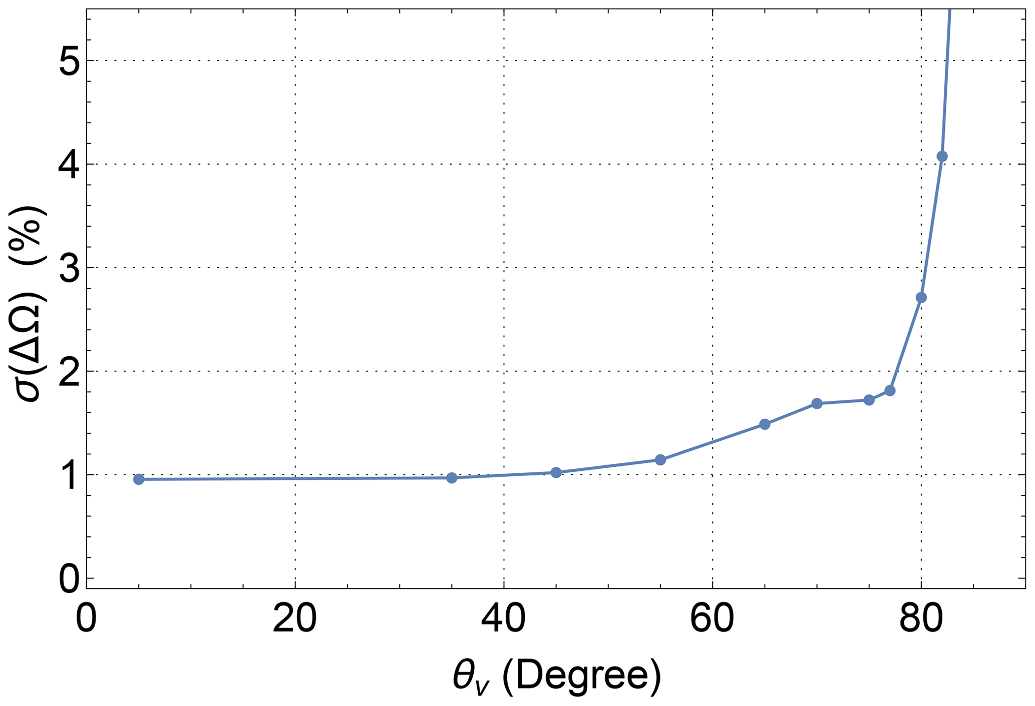
Figure 19 The standard deviation (σ) of O₃ errors due to profile mismatches as a function of the viewing zenith angle (θ_v), estimated using the M2TCO3 profile covariance matrix for the December midlatitude zone (40–50^∘ N).

Retrieval of SO₂ requires knowledge of the altitude at the center of the volcanic plume, which can be represented by a narrow (e.g., a width of 1.5 km) GDF. Error in the plume altitude leads to SO₂ retrieval error, which can be estimated using the retrieval AK. Figure 18b and d show sample AKs and their variations with VZA for an SO₂ plume center at 11 km altitude. The values of these AKs are equal to 1 at 11 km, meaning no retrieval error when the altitude used in the retrieval is equal to the actual plume altitude. Here, we examine the case of a low-reflectivity surface. The retrieved SO₂ column overestimates (underestimates) the actual column when the plume altitude is higher (lower) than the assumed altitude (11 km). At low VZAs (<35^∘), AK values are close to 1 above the assumed altitude (11 km), indicating small (less than a few percents) errors for plumes at higher altitudes. Overestimation (up to 150 %) increases quickly with larger VZAs when the plume is at higher altitudes. Underestimation is more severe with a lower altitude of the plume: 10 % to 20 % per 1 km lower than the assumed altitude.

6.2.5 Errors from Lambertian treatment of natural surfaces

Reflections from surfaces are anisotropic but treated as isotropic. To estimate errors in O₃ and SO₂ columns due to this simplification, we performed DVCF retrieval from simulated radiances. First, TOA radiances of the four EPIC UV bands are modeled using a state-of-art radiative transfer model, VLIDORT (Spurr, 2006), for a molecular atmosphere with various O₃ and SO₂ profiles over a surface characterized by an anisotropic BRDF. Next, GLERs are determined at the long wavelength bands (B3 and B4) and then linearly extrapolated to the short wavelength bands (B1 and B2). Finally, retrieved O₃ and SO₂ columns from simulated B1 and B2 radiances using the extrapolated GLERs are compared with the column settings of the forward modeling to quantify retrieval errors. Examples of O₃ and SO₂ errors determined this way are shown in Fig. 20 for observing conditions described in the Fig. 4 caption. In the closed-loop testing, surface reflection is specified by the Cox–Munk BRDF, which is highly anisotropic, more so than the land surface BRDFs that are well-characterized by the combinations of Lambertian, Ross, and Li kernels (Lucht et al., 2000; Schaaf et al., 2011). Hence, the Cox–Munk BRDF selection provides error ranges due to the Lambertian treatment of surface reflections. Closed-loop tests are performed for a wide range of viewing illumination geometries and vertical distributions of O₃ and SO₂. Test results (see, e.g., Fig. 20) show that errors in total O₃ are mostly within ±1 DU, while SO₂ errors are within ±5 % for SO₂ layers above 5 km, and decrease (increase) with higher (lower) layer altitudes. As shown in Fig. 5, the AMF errors due to Lambertian treatment occur below 20 km altitude. Consequently, a small fraction of the O₃ profile is affected by this approximation. Thus, O₃ errors are proportional to the tropospheric columns but are insensitive to the total column amounts. Since a vast majority of volcanic SO₂ clouds are located below 20 km altitude, SO₂ errors are proportional to the total SO₂ columns. Higher SO₂ clouds are not affected by this treatment.

Figure 20 Errors in retrieved O₃ and SO₂ due to Lambertian surface treatment of an anisotropic surface. (a) O₃ errors in DU for a midlatitude O₃ profile with total columns of 275, 375, and 475 DU. (b) SO₂ errors in percent for an SO₂ layer at altitudes of 5, 7, and 11 km above sea level. See the Fig. 4 caption for the specification of surface BRDF and viewing and illumination geometry.

6.2.6 Errors from MLER treatment of clouds and aerosols

The MLER model is adopted to treat atmospheric particles, including clouds and aerosols, which predominantly reside in the lower troposphere. The modeled light paths (especially in the troposphere) based on this treatment differ significantly from those for light transfer through the particle-laden atmosphere (see, e.g., Fig. 9). The retrieval errors due to this simplification are again estimated using closed-loop testing. First, TOA radiances of the EPIC UV bands are simulated using VLIDORT for particle-laden atmospheres with various O₃ and SO₂ profiles over Lambertian surfaces of different reflectivities. Then inversion from the simulated radiances with the MLER treatment permits the identification of conditions under which retrieval errors are significant.

Clouds

The error in total O₃ due to the MLER treatment of a low-lying (below 10 km) cloud is mostly within ±2 DU (e.g., Fig. 21a). This O₃ error decreases slightly with a lower cloud altitude (or higher cloud pressure) but is insensitive to the cloud fraction or the total O₃ column. In other words, the MLER treatment does not contribute to large uncertainty in the retrieved total O₃ column, provided that an accurate OCP for the cloud is used for the MLER cloud surface. However, OCP has some uncertainty, contributing to additional uncertainty in the O₃ column: a low (high) bias in OCP results in a positive (negative) error in total O₃; quantitatively, ±100 hPa causes about ∓4 DU (see Fig. 21a). The OCP uncertainty is estimated to be within ±50 hPa, thus contributing ∓2 DU to the total O₃ uncertainty. Combining O₃ uncertainties due to the OCP error and the MLER treatment yields ±4 DU uncertainty in total O₃ under cloudy conditions.

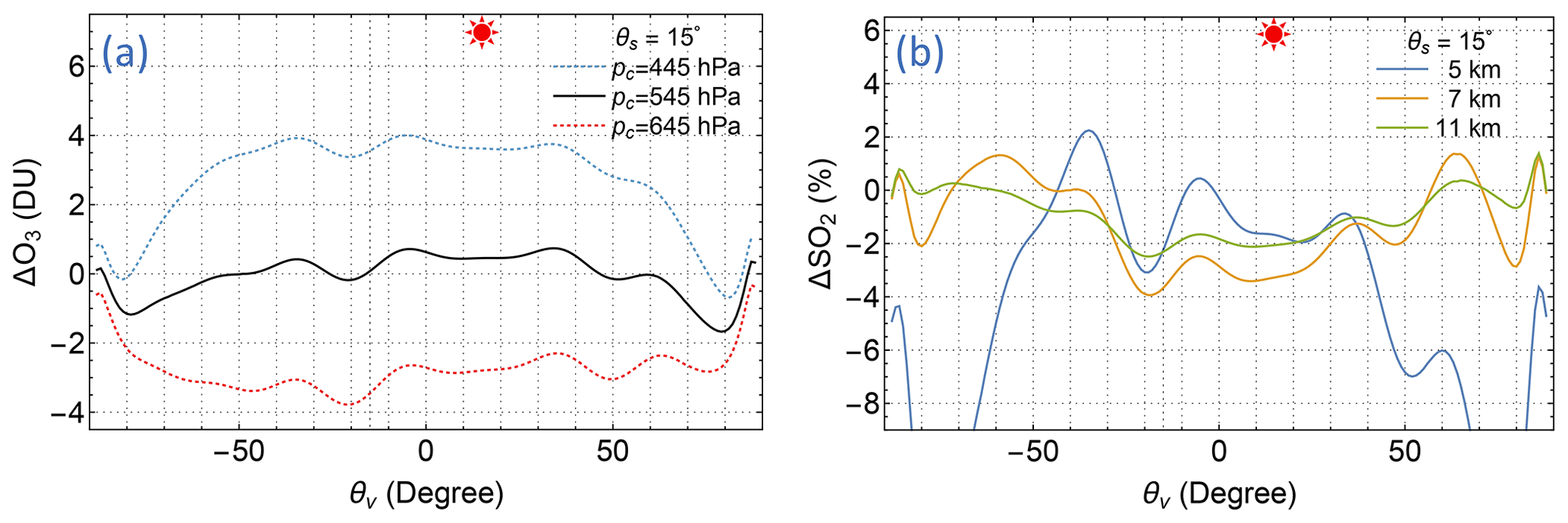
Figure 21 Errors in retrieved O₃ and SO₂ due to MLER treatment of clouds, which are represented by 1.5 km thick C1 particle layers with an optical thickness τ=15 at 340 nm. (a) O₃ errors in DU for correct (p_c=545 hPa) and biased ($p_{\mathrm{c}}=\mathrm{545}\pm \mathrm{100}$ hPa) cloud OCPs. (b) SO₂ errors in percent for SO₂ layers at three altitudes (5, 7, and 11 km) above a layer of cloud (at 3 km altitude). See the Fig. 4 caption for the specification of viewing and illumination geometry.

The error in the total SO₂ column due to the MLER cloud treatment is within ±2 % when the SO₂ layer in the troposphere is well above the underlying cloud. This SO₂ error increases with a smaller separation between the SO₂ layer and the cloud, reaching ±15 % when the SO₂ layer is just above the cloud. These characteristics of SO₂ error are illustrated in Fig. 21b. In contrast to the MLER treatment O₃ error, which is insensitive to the total column, this SO₂ error is proportional to the total SO₂ column. When the SO₂ layer is below or within the cloud, the uncertainty of SO₂ quantification increases drastically. Depending on the relative distributions of SO₂ and the cloud particles, the retrieved SO₂ based on the MLER treatment can be a fraction of or a few times the actual column.

Aerosols

Besides clouds, the MLER treatment is applied to IFOVs contaminated by aerosols, which primarily reside in the troposphere and cover a significant portion of Earth's surface. These aerosols are suspended tiny (micron-scale) particles that scatter and possibly absorb sunlight. The frequently observed non-absorbing (or weakly absorbing) aerosols are sea salt and sulfate (SLF), and UV-absorbing aerosols are smoke (i.e., carbonaceous aerosols from biomass combustion, BIO), mineral dust (DST), and volcanic ash. Moderate and high positive AI values indicate the presence of UV-absorbing aerosols in an IFOV, while negative and slightly positive AI values indicate the presence of non-absorbing or weakly absorbing aerosols.

Closed-loop testing shows that MLER treatment of non-absorbing and weakly absorbing aerosols in the lower troposphere (<7 km) results in small ($<\pm \mathrm{2}$ DU) errors in total O₃ retrievals, provided that the proper OCP for the elevated cloud surface is used. This error range is nearly independent of the total O₃ column or the aerosol loading.

The MLER treatment errors for UV-absorbing aerosols close to the surface (<1 km altitude) are mostly within ±1 DU, similar to the error range associated with the LER treatment of BRDF surfaces. For elevated UV-absorbing aerosols, the MLER treatment and the linear r_gf_c extrapolation scheme (see Sect. 2.3) result in a positive bias in the retrieved total O₃ columns (see, e.g., Fig. 22). This O₃ bias depends on the viewing illumination geometry and generally increases with stronger aerosol absorption (i.e., lower single-scattering albedo, ω), larger aerosol optical thickness, and higher altitude of aerosol layers. Regression analysis of results from closed-testing with many combinations of viewing illumination geometries, particle-laden atmospheres (with various optical properties, optical thicknesses, and vertical distributions), surface reflectivities, and O₃ profiles reveals a positive correlation between column O₃ error and the UV AI. Quantitatively, this relationship can be written as $\mathrm{\Delta }{\mathrm{O}}_{\mathrm{3}}=(\mathrm{1.5}\pm \mathrm{1})\times \mathrm{AI}$ DU for AI values greater than 0.5 and less than 8. This relationship provides a rough estimate of O₃ bias based on the observed AI. Typically, AI values fall between 1 and 4 with a median value of 1.5 for EPIC observations of UV-absorbing aerosols, corresponding to a mean O₃ bias of about 3 DU for IFOVs contaminated with UV-absorbing aerosols. The MLER treatment sometimes fails when aerosol absorption is strong such that the derived LER becomes negative. In this case, the explicit aerosol treatment may be needed to reduce the retrieval uncertainty.

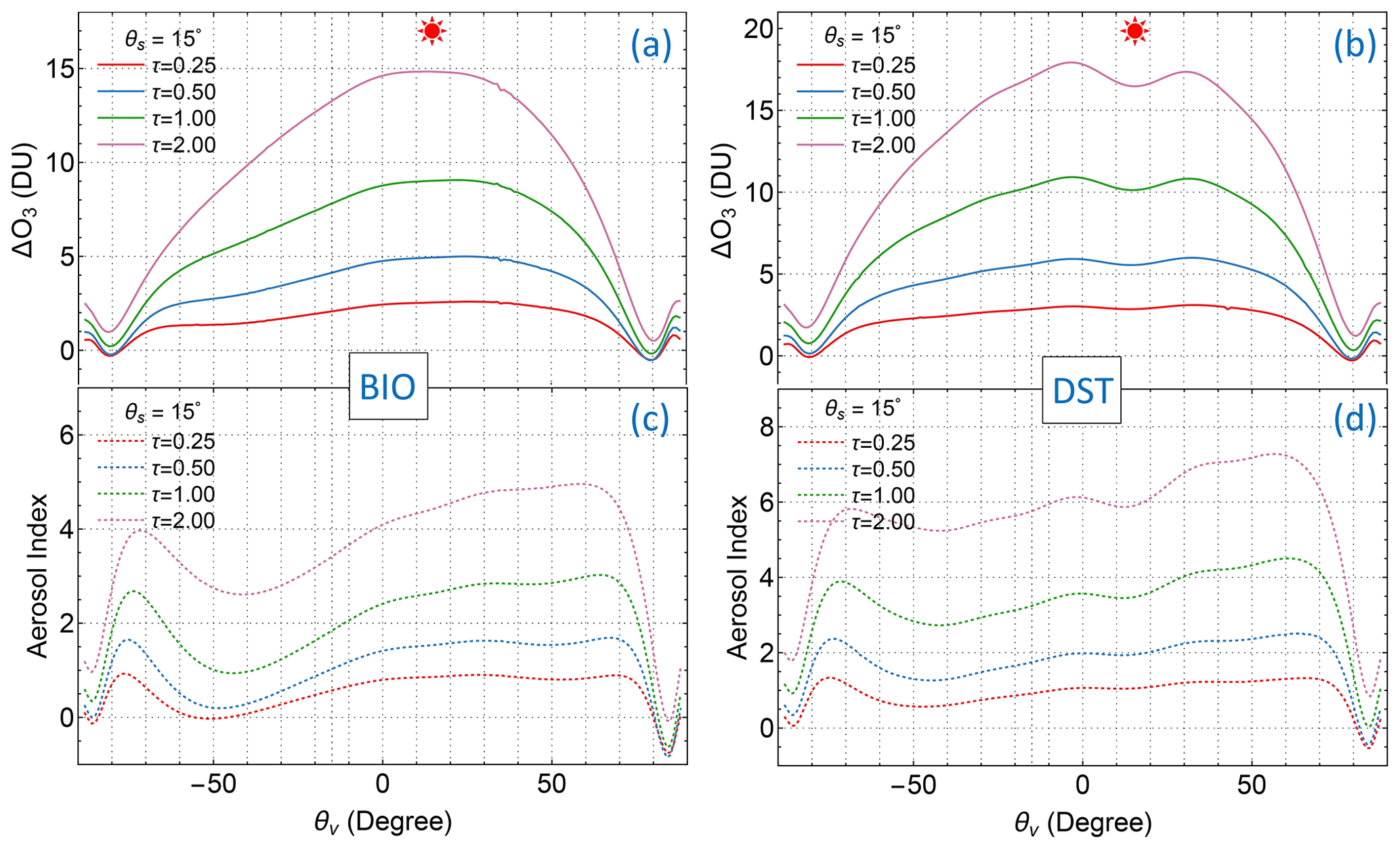
Figure 22 Errors in retrieved O₃ due to MLER treatment of two common UV-absorbing aerosols, (a) BIO (ω=0.921) and (b) DST (ω=0.900), with various optical thicknesses (τ = 0.25, 0.5, 1.0, and 2.0 at 340 nm) located at 5 km altitude. See the Fig. 4 caption for the specification of viewing and illumination geometry. The AIs associated with each observation scenario are shown in (c) and (d).

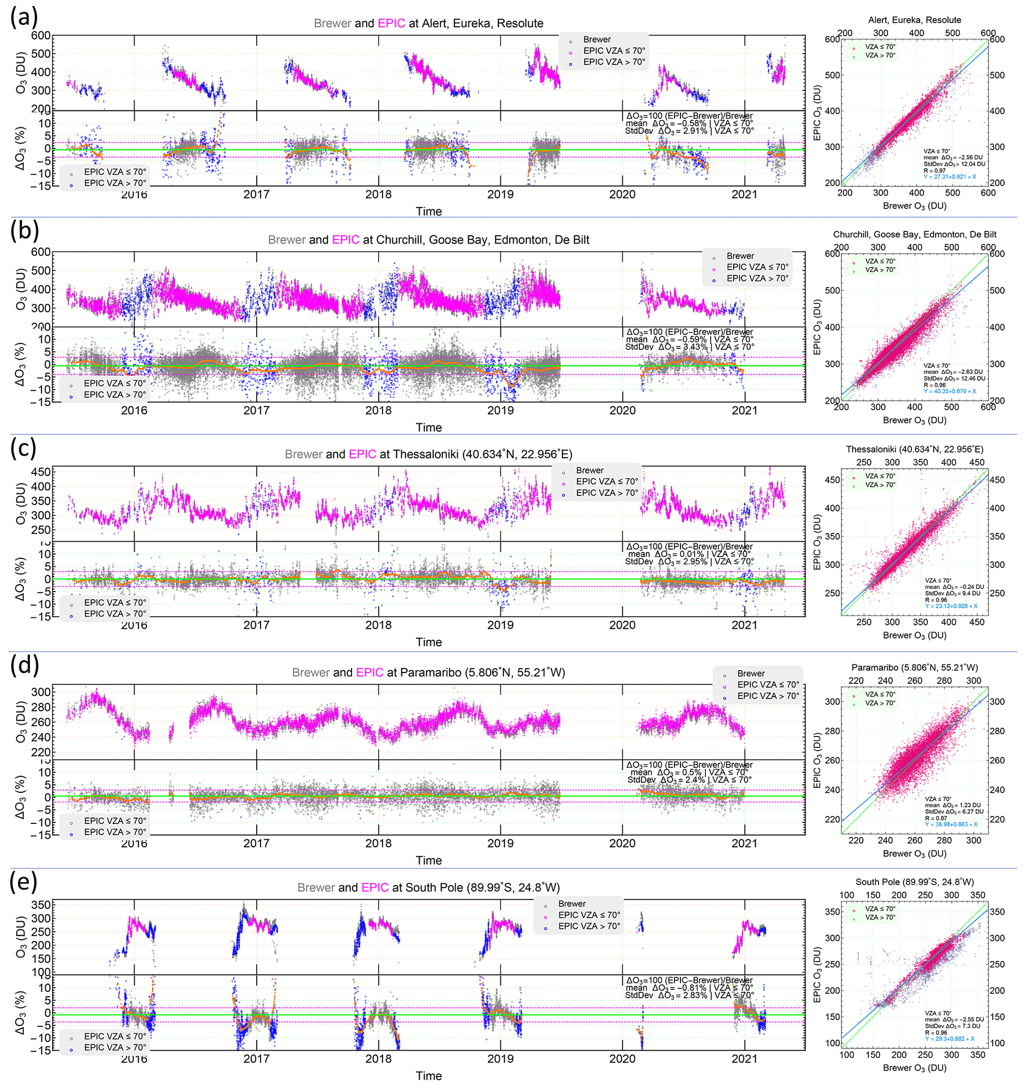
Figure 23 Intercomparison of total O₃ from EPIC and the ground-based Brewer spectrophotometers from July 2015 to April 2021 at 10 selected ground stations with high-cadence measurements: Alert (82.50^∘ N), Eureka (79.99^∘ N), Resolute (74.72^∘ N), Churchill (58.75^∘ N), Edmonton (53.55^∘ N), Goose Bay (53.31^∘ N), De Bilt (52.10^∘ N), Thessaloniki (40.63^∘ N), Paramaribo (5.806^∘ N), and the South Pole (−89.99^∘ N). EPIC and Brewer coincident pairs are used in the plots, and data with VZA $\le \mathrm{70}{}^{\circ }$ N only are included in the difference statistics.

EPIC's high-cadence observation has more chances to view volcanic clouds during or soon after eruptions. These young volcanic clouds contain mixtures of ash particles and water or ice clouds, as eruptions inject ash and gases (including SO₂) into the atmosphere. Since ash particles strongly absorb UV, the MLER treatment of volcanic plumes leads to huge uncertainties in the retrieved SO₂ columns, which are often greatly overestimated or underestimated depending on the relative distributions between SO₂ and ash particles. An explicit treatment of volcanic ash is needed for accurate retrieval of SO₂ when ash particles are co-located with or slightly separated from the gas.

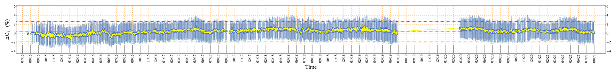
Figure 24 Comparison of synoptic EPIC O₃ with MERRA-2 assimilated O₃: time series of mean daily differences and standard deviations for EPIC observations with VZA ≤70^∘.

6.3 Error summary

Uncertainty estimates (Sect. 6.2) have detailed various contributions to systematic and random errors in retrieved O₃ and SO₂ vertical columns. In this summary, these error types are separately combined to estimate their total systematic and random errors, respectively.

First, random errors from various sources, including measurement noise and errors in temperature profiles and O₃ vertical profiles, are combined to estimate total random errors. The random O₃ error (characterized by its standard deviation) is 1.5 % at low VZAs ($<\mathrm{45}{}^{\circ }$), increasing to 2.0 % at 75^∘ for IFOVs without clouds and aerosols. Similarly for IFOVs with clouds or non-absorbing aerosols, the random error in the total O₃ column is 1.8 % for low VZAs ($<\mathrm{45}{}^{\circ }$) and 2.5 % at 75^∘. Random SO₂ error has two terms: one is independent of the SO₂ column (see Sect. 6.2.1), but the other is proportional to this column (see Sect. 6.2.2). Hence, they are not combined.

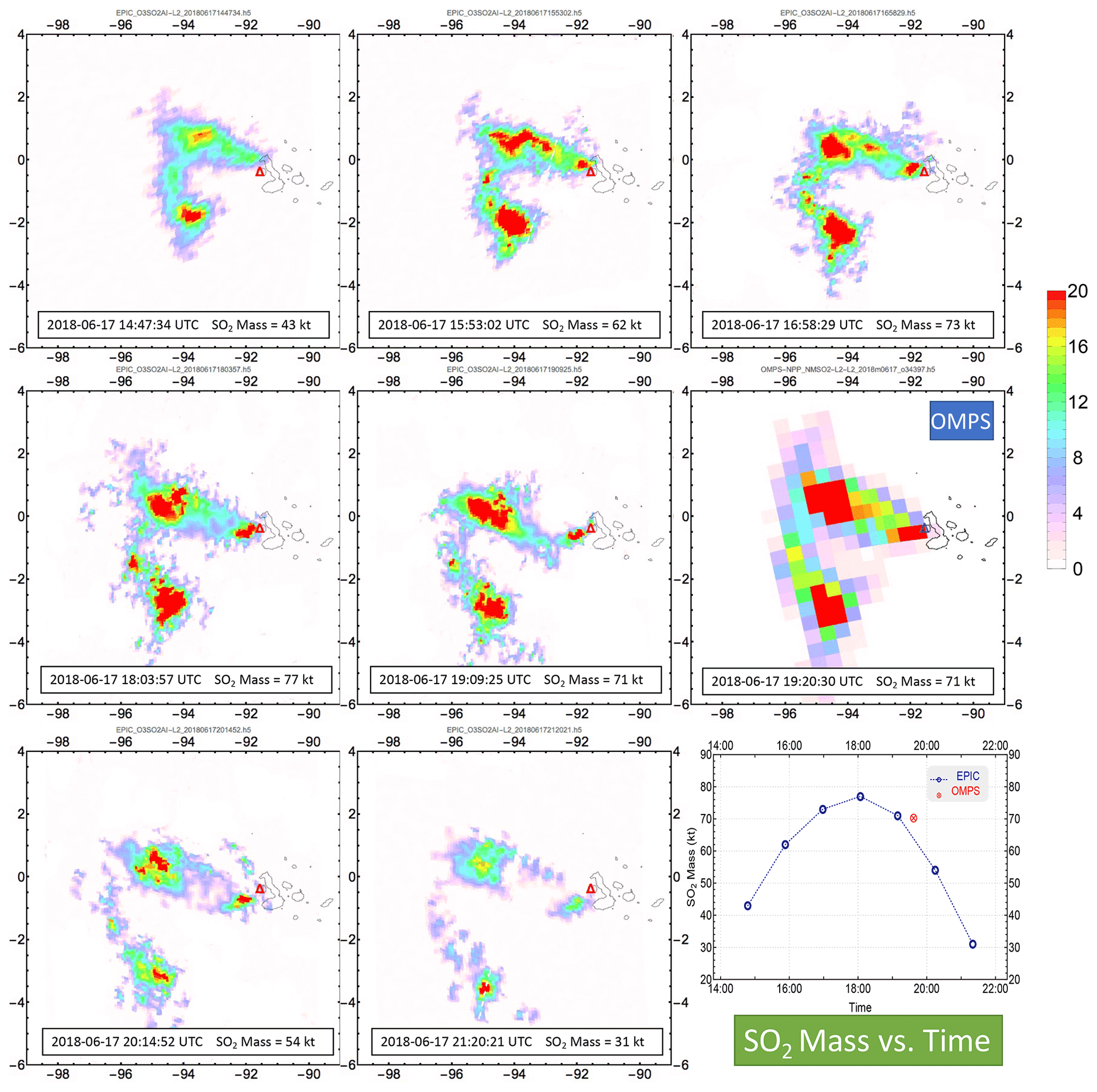
Figure 25 EPIC and OMPS observations of volcanic SO₂ plumes on 17 June 2018 from the eruption of Fernandina volcano (Δ) in the Galapagos Islands. This eruption injected a significant amount of SO₂ into the troposphere at about 3.5 km above sea level. The mass loading of an SO₂ plume is obtained by summing the SO₂ masses of all IFOVs with SO₂ vertical columns ≥1 DU. The lower right panel plots the EPIC and OMPS SO₂ masses vs. the observation time (UTC).

Next, the radiometric biases, forward radiance modeling errors, and errors in molecular cross-sections are the primary contributions to the systematic errors in the retrieved vertical columns. The possible ranges due to these sources are provided earlier in this section, but their actual contributions are unknown. We obtain the total systematic error by combining the likely ranges (i.e., ∼half of the possible ranges) of these contributions and estimate the bias in the total O₃ column to be ±2 % for VZA $\le \mathrm{70}{}^{\circ }$ and ±3.5 % for VZA $\le \mathrm{85}{}^{\circ }$; the bias in the total SO₂ column high (>10 km) in the atmosphere is estimated to be ±1.5 % for VZA $\le \mathrm{70}{}^{\circ }$ and ±5 % for VZA $\le \mathrm{85}{}^{\circ }$. Some biases depend on geophysical conditions. For instance, O₃ has a positive bias for IFOVs with UV-absorbing aerosols, increasing with a higher AI (see Sect. 6.2.6). Underestimation (overestimation) of an SO₂ column occurs when its layer altitude used in the retrieval is higher (lower) than the actual altitude (see Sect. 6.2.3).

7 Validation of EPIC O₃ and comparison of SO₂

7.1 O₃ validation

We validate the DVCF O₃ retrievals from EPIC using ground-based Brewer spectrophotometer measurements and the assimilated O₃ product from MERRA-2, the Modern-Era Retrospective Analysis for Research and Applications Version 2 (Gelaro et al., 2017).

We compare EPIC total O₃ columns with the Brewer O₃ data at 10 selected ground stations with high-cadence measurements distributed in five latitude zones. At each of these selected stations, a Brewer spectrometer makes a measurement every few (∼10) minutes during the daylight hours each day, thus providing total vertical O₃ columns that are coincident (within ±15 min) with EPIC observations at these stations. For intercomparison, Brewer O₃ data are interpolated to the times when EPIC observes these locations. Coincident O₃ data from these two independent sources are displayed in the upper panels of Fig. 23a–e, their differences in the lower panels of Fig. 23a–e, and the EPIC vs. Brewer scatter plots in the right panels of Fig. 23a–e. We include coincident data with VZA ≤70^∘ only for statistical analysis due to EPIC–Brewer IFOV differences that usually increase with slant path lengths and EPIC's footprint sizes as well as due to calibration biases at large VZAs or SZAs. The mean difference and standard deviations in percent are displayed in the difference plots, while those in DU and the correlation coefficients are in the scatter plots. Time series of O₃ difference (see lower panels of Fig. 23a–e between EPIC and Brewer) are highly stable with similar moving averages and standard deviations from June 2015 to April 2021, showing that EPIC O₃ is consistent over time, without noticeable drift. The correlations between EPIC and Brewer are very high with correlation coefficients R≥0.96 for most stations (except for the Paramaribo station near the Equator, where R=0.87), demonstrating that EPIC captures O₃ variability accurately. EPIC O₃ agrees with the Brewer measurements to better than 1 % with standard deviations of differences less than 3.5 % for all the ground stations, validating the high accuracy of EPIC total O₃.

From October 2004, MERRA-2 O₃ field is assimilated from Aura MLS and OMI and provides highly realistic global distributions of O₃ in the stratosphere and upper troposphere while inheriting the uncertainty characteristics of its sources (Stajner et al., 2008; Wargan et al., 2015; Davis et al., 2017). We compare the MERRA-2 synoptic O₃ field with the EPIC hemispheric view for the same observation time to access EPIC's capability of capturing the realistic O₃ distribution. For instance, strikingly similar O₃ spatial distributions are observed in EPIC measurements (Fig. 15c) and the MERRA-2 assimilation (Fig. 15d), with agreement at $-\mathrm{0.20}\pm \mathrm{2.52}$ % (or $-\mathrm{0.35}\pm \mathrm{5.6}$ DU; Fig. 15h). We expand this synoptic comparison to each EPIC hemispheric view obtained from July 2015 to August 2021 and plot in Fig. 24 the time series of daily statistics. This time series shows that nearly the same level of agreement is achieved for the entire period, with a mean bias and standard deviation of 0.44±2.19 % (or 1.16±6.34 DU). Considering the mean bias (about −1.2 %) of MERRA-2 total O₃ (Wargan et al., 2017), we estimate the accuracy of EPIC total O₃ to be $-\mathrm{0.76}\pm \mathrm{2.19}$ %.

7.2 SO₂ comparison

Volcanic eruptions occur sporadically and without warning, but EPIC on DSCOVR, from the unique L1 vantage point, usually provides multiple daily observations of volcanic SO₂ and ash clouds once injected into the atmosphere. In contrast, ground-based instruments rarely detect volcanic clouds unless they drift over one in operation. We thus rely on polar-orbiting instruments, which may observe a volcanic cloud once (or more at high latitude) per day to provide validation measurements.

The OMPS-NM on SNPP provides high-quality hyperspectral measurements in the UV, from which highly accurate retrievals of O₃ and SO₂ are achieved using the DVCF algorithm. The DVCF algorithm can apply to both discrete spectral measurements (e.g., TOMS and EPIC) and hyperspectral ones (e.g., OMI and OMPS-NM). The main difference is that more information can be extracted from hyperspectral measurements to improve the accuracy and precision of the retrieved geophysical parameters. For instance, the altitude of an SO₂ layer can be determined in addition to its amount simultaneously using the DVCF algorithm (Yang et al., 2010). Having the altitude information significantly improves the accuracy of SO₂ quantification because the SO₂ measurement sensitivity varies strongly with its altitude. Thus, DVCF height-resolved SO₂ retrievals from hyperspectral instruments, such as OMI and OMPS-NM, provide the most accurate quantification of SO₂ vertical columns. To validate DVCF SO₂ retrievals from EPIC, we compare the SO₂ mass loading of a volcanic plume integrated from EPIC observations with SNPP OMPS-NM for the same event.

Figure 25 compares the DVCF retrievals of the volcanic plume from the explosive eruption of Fernandina volcano in the Galapagos Islands on 17 June 2018. Seven plume exposures about 65 min apart are taken by EPIC on this day. Soon after the fifth EPIC exposure, the OMPS observed this plume for the first time. For the exposures at 10 min apart, both instruments estimate the mass loading at 71 kt, validating the EPIC SO₂ result.

The lower right panel of Fig. 25 plots the plume mass vs. the observation time, showing the mass loading peaks near local noontime. The observed mass change results from the continuing emission from the volcano, the conversion of SO₂ into sulfate, and the changing measurement sensitivity with viewing illumination conditions since low SO₂ columns may be missed at large (VZA, SZA, or both) angles due to lower sensitivity. EPIC's high-cadence observations allow better identification of the peak loading of volcanic SO₂ plume, thus usually providing more accurate estimates of the lower bound of SO₂ emission compared to polar-orbiting instruments.

We have conducted many mass loading comparisons between EPIC and OMPS and found that the agreements are usually within 20 %. These findings indicate that DVCF SO₂ retrieval from EPIC provides better than 20 % (an estimate of the upper error bound) accuracy in total mass for eruptions with greater than 50 kt emissions.

8 Conclusions

We present the algorithm for making the EPIC O3SO2AI product in this paper. This algorithm is based on the DVCF algorithm developed for retrieving trace gases, including O₃, SO₂, and NO₂, from Aura OMI and Suomi NPP as well as NOAA-20 OMPS. Algorithm advances, including the improved O₃ profile representation and the regulated direct fitting inversion technique, improve the accuracy of O₃ and SO₂ from the multi-channel measurements of DSCOVR EPIC. The theoretical basis of the SOE approach, introduced to reduce retrieval artifacts due to EPIC's band-to-band misregistration, can be exploited for other applications, such as the separation of a spatially smooth data field (e.g., stratospheric O₃) from that (e.g., tropospheric O₃) with higher spatial variations.

A thorough error analysis is provided to quantify O₃ and SO₂ retrieval uncertainties due to various error sources and simplified algorithm physics treatments. Error analysis findings indicate that the MLER treatment of UV-absorbing aerosols leads to significant uncertainties in retrieved O₃ and SO₂ columns. Future improvements may include explicit aerosol treatment or other schemes for radiance or product corrections. The GLER treatment of anisotropic surface reflections introduces small errors in the retrieved total O₃ and SO₂ columns, primarily because surface reflection is a minor component of measured radiance in the UV. However, this GLER treatment does not generally provide a more accurate tropospheric AMF. Hence, explicit BRDF treatment of surface reflection is needed for accurate retrievals of tropospheric gases.

The EPIC total O₃ columns are validated against coincident ground-based Brewer measurements and compared with coincident O₃ data from MERRA-2 assimilation. The findings show that EPIC total O₃ is highly accurate, realistically capturing the short-term O₃ variability while maintaining long-term consistency over the entire record. The EPIC SO₂ loadings of volcanic plumes are evaluated against those from hyperspectral measurements of the same eruptions, showing that EPIC provides accurate SO₂ quantifications from large volcanic eruptions. EPIC's high-cadence observations allow better identification of the peak loading of volcanic SO₂ plumes compared to polar-orbiting instruments.