the Creative Commons Attribution 4.0 License.
the Creative Commons Attribution 4.0 License.
 | 21 Oct 2022
DeepPrecip: a deep neural network for precipitation retrievals
George Duffy
Lisa Milani
Christopher G. Fletcher
Claire Pettersen
Kerstin Ebell
Remotely-sensed precipitation retrievals are critical for advancing our understanding of global energy and hydrologic cycles in remote regions. Radar reflectivity profiles of the lower atmosphere are commonly linked to precipitation through empirical power laws, but these relationships are tightly coupled to particle microphysical assumptions that do not generalize well to different regional climates. Here, we develop a robust, highly generalized precipitation retrieval algorithm from a deep convolutional neural network (DeepPrecip) to estimate 20 min average surface precipitation accumulation using near-surface radar data inputs. DeepPrecip displays a high retrieval skill and can accurately model total precipitation accumulation, with a mean square error (MSE) 160 % lower, on average, than current methods. DeepPrecip also outperforms a less complex machine learning retrieval algorithm, demonstrating the value of deep learning when applied to precipitation retrievals. Predictor importance analyses suggest that a combination of both near-surface (below 1 km) and higher-altitude (1.5–2 km) radar measurements are the primary features contributing to retrieval accuracy. Further, DeepPrecip closely captures total precipitation accumulation magnitudes and variability across nine distinct locations without requiring any explicit descriptions of particle microphysics or geospatial covariates. This research reveals the important role for deep learning in extracting relevant information about precipitation from atmospheric radar retrievals.
- Article
(4166 KB) - Full-text XML
- BibTeX
- EndNote


Accurate estimates of surface precipitation are highly sought-after as they inform flood forecasting operations, water resource management practices and energy planning (Buttle et al., 2016; Gergel et al., 2017). Due to the sparse nature of in situ precipitation measurement networks, remote sensing has become a prominent alternative source of observations for deriving surface precipitation estimates (Liu, 2008). Ground-based scanning radars are valuable resources as they provide estimates of precipitation over a wider area and at a higher temporal resolution compared to traditional in situ gauges (Lemonnier et al., 2019). Additionally, the size and availability of both vertically pointing and space-borne remote sensing datasets have expanded greatly in recent decades as a result of technological instrument improvements and new satellite missions (Quirita et al., 2017).
Remotely sensed radar observations used in empirical, power law relationships can relate radar reflectivity (RFL) estimates (Ze) to surface snowfall (S) or rainfall (R) rates (Eq. 1) (Matrosov et al., 2008; Kulie and Bennartz, 2009; Schoger et al., 2021):
These radar-based retrievals are powerful tools for filling current observational gaps and have been applied to great effect in previous literature (Levizzani et al., 2011; Hiley et al., 2010). However, these relationships demonstrate an inability to generalize well to unseen validation data as a consequence of the microphysical particle assumptions (e.g. shape, diameter, particle size distribution (PSD), terminal fall velocity and mass) used in each relationship's unique derivation (Jameson and Kostinski, 2002).
Recent machine learning (ML) approaches have demonstrated improvements in estimating surface precipitation from remotely sensed data compared to traditional nowcasting methods (Shi et al., 2017; Kim and Bae, 2017). Deep learning models have benefited greatly from the increased observational sample provided by remote sensing missions and have shown skill in learning complex spatiotemporal characteristics of the underlying datasets (L. Chen et al., 2020). However, a deep learning convolutional surface precipitation retrieval using vertical column radar data with no spatiotemporal covariates has yet to be developed to our knowledge. Previous ML studies typically focused on passive microwave and infrared datasets, which lack a detailed analysis of the vertical column structure or suffer from a limited sample for model training across multiple, distinct regional climates (Xiao et al., 1998; Adhikari et al., 2020; Ehsani et al., 2021).
In this work, we evaluate the abilities of a novel deep learning precipitation retrieval algorithm trained on vertically pointing radar (up to 3 km above the surface). The regression model that we present (DeepPrecip) is a hybrid deep learning neural network consisting of a feature extraction convolutional neural network (CNN) front-end and a regression feedforward multilayer perceptron (MLP) back-end. The combination of these two architectures allows DeepPrecip to recognize and learn the non-linear relationships between different layers in the vertical column of radar observations and produce an accurate surface precipitation estimate. Through an analysis of feature input combinations, the performance of DeepPrecip is examined to identify regions within the vertical column that contain the most important contributions to retrieval accuracy (Lundberg and Lee, 2017). The relationships that exist between different layers of the vertical profile (and each atmospheric covariate) can be used to help inform current and future active radar retrievals of surface precipitation.
2.1 Study sites
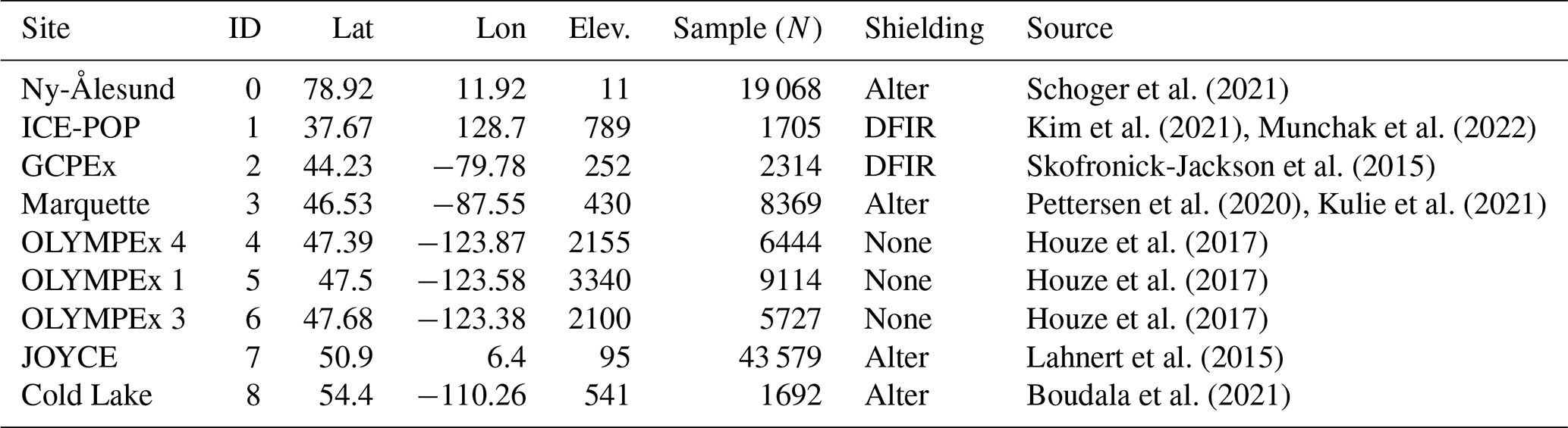
In situ data was collected from nine study sites (Fig. 1a) from 2012–2020 (Table 1). Colored markers in Fig. 1b indicate periods where non-zero surface precipitation was recorded. Study sites were selected based on the required presence of a micro rain radar (MRR) and collocated Pluvio2 weighted precipitation gauge. Rain, snow, and mixed-phase precipitation were recorded, with each site's precipitation phase and intensity distribution of observations differing based on the regional climate. For instance, Marquette experienced strong lake-effect snowfall, while Cold Lake received mostly light, shallow snowfall. Further, due to the warmer temperatures recorded at OLYMPEx, these sites were classified as primarily experiencing liquid precipitation, while ICE-POP received only solid precipitation.
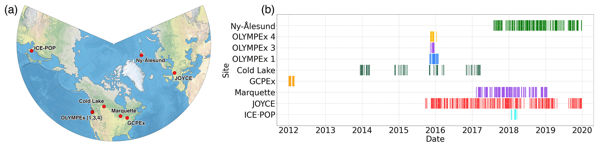
Figure 1Observational input data locations and temporal coverage periods. (a) Geographic study site locations. (b) Timeline of observational coverage (periods of active precipitation) for each site from 2012 to 2020.
Table 1Summary of in situ study site locations, identifiers, and observational details.
2.2 Pluvio2 precipitation weighing gauge
Reference surface precipitation observations were collected by OTT Pluvio2 weighted gauges at each site. The Pluvio2 gauge records the precipitation accumulation from falling hydrometeors with a minimum time resolution of 1 min (Colli et al., 2014). It includes a 200 cm2 heated surface orifice (400 cm2 at Ny-Ålesund) to prevent snow and ice buildup, along with site-specific wind shielding implemented as described in Table 1. These fence setups include a Double Fence Intercomparison Reference (DFIR) shield, which is a large, double-fenced wooden structure that helps significantly reduce the impact of wind on surface precipitation measurements (Rasmussen et al., 2012; Kochendorfer et al., 2022). The Alter shield system consists of multiple freely hanging, spaced metal slats around the gauge top opening, which also helps mitigate undercatch issues during strong winds (Colli et al., 2014). Sensitivity analyses of different rolling temporal windows indicated an optimal temporal resolution of 20 min non-real time accumulation (measurement results 5 min after precipitation accumulation), with minimum observational thresholds of at least 0.2 mm over the course of an hour from the Pluvio2 gauge.
2.3 Micro rain radar
Vertical pointing MRRs (developed by METEK) were located near the Pluvio2 gauges at each site to record complementary atmospheric observations. The MRR is a K-band (24 GHz) continuous wave Doppler radar that provides information related to hydrometeor particle activity up to 3.1 km above the surface (or 1 km for Ny-Ålesund) as a function of spectral power backscatter intensity. The MRR provides 29 vertical bins (of size 100 m) spanning 300 to 3100 m above the surface as shown for each site in Fig. 2a. Raw radar measurements were preprocessed using Maahn's improved MRR processing tool (IMProToo) for noise removal, dealiasing, and for extending the minimum detectable dBZ to −14, which allows for improved measurements of solid precipitation. This data was then temporally averaged to align to the same 20 min windows generated for the Pluvio2 observations and used as a model input (Maahn and Kollias, 2012).
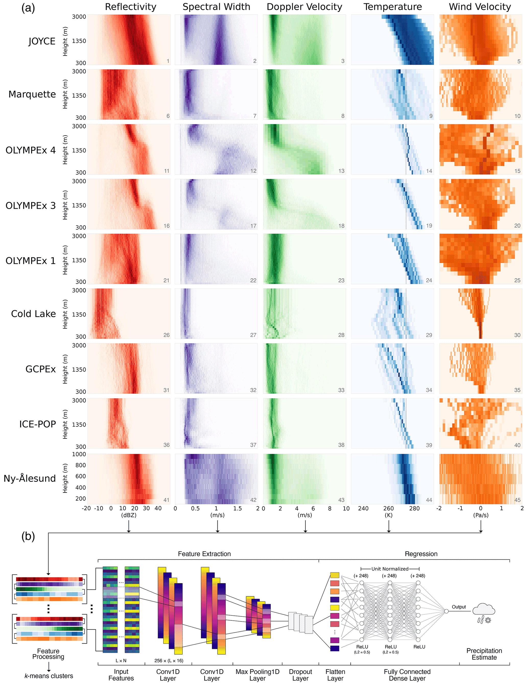
Figure 2DeepPrecip input covariates, feature processing pipeline, and model architecture. (a) Site-predictor matrix of normalized Micro Rain Radar (MRR) and ERA5 observational frequency histograms used in model training and testing. Note that darker colors in the 2D heatmaps indicate a higher frequency of observations. (b) DeepPrecip convolutional neural network diagram for L inputs with N predictors.
2.4 ERA5
European Centre for Medium-Range Weather Forecasts Reanalysis version 5 (ERA5) hourly temperature (TMP) and vertical wind velocity (WVL) on pressure levels from 0 to 3 km were also included as additional input covariates to DeepPrecip (Hersbach et al., 2020). These inputs allow the model to more accurately recognize different precipitation event structures, large-scale atmospheric dynamics, and hydrometeor phases during training. Note that WVL units (Pa s−1) are defined using the ECMWF Integrated Forecasting System (IFS), which adopts a pressure-based vertical co-ordinate system (i.e. negative values indicate upwards air motion, since pressure decreases with height). Each of these variables were linearly interpolated to align with the MRR data over 20-min intervals and at 100 m vertical resolution.
2.5 Surface meteorology
Collocated surface temperature (degrees Celsius, ∘C) and 10 m wind speed (m s−1) meteorologic observations were also collected from instruments installed at each site and temporally aligned to the Pluvio2 and MRR datasets. Surface wind data acts as an additional observational constraint for mitigating the effects of undercatch on unshielded measurement gauges (Rasmussen et al., 2012). Undercatch occurs when precipitation falling in the presence of wind can cause hydrometeors to pass over the gauge top orifice. This effect has been shown to bias reported precipitation quantities by up to 10 % (Ehsani and Behrangi, 2022). We therefore limit the available training dataset to periods when surface wind speeds are <5 m s−1, as this restricts the analysis to low-medium wind speed events at each location to maintain a high gauge-catch efficiency (Yang, 2014). This preprocessing step reduces the average size of our total observational pool by 16 % across all stations; however, we note that maximum intensity precipitation events are not removed using this technique.
Surface meteorologic station temperature data is used for precipitation-phase partitioning at 5 ∘C to allow for comparisons with DeepPrecip. Additional dry surface air temperature thresholds of 0, 1, and 2 ∘C were also examined, but performance for both rain and snow appeared optimal when classified using a 5 ∘C threshold (where temperatures <5 ∘C are considered as solid precipitation, and temperatures >=5 ∘C are considered as rainfall). This simple temperature threshold is an additional source of uncertainty in our comparisons with the relationships due to the influence of mixed-phase precipitation on power law accuracy, along with uncertainties in the location of the active melting layer (Jennings et al., 2018). A more sophisticated phase partitioning system (e.g. using wet-bulb temperature as described in Sims and Liu, 2015) could also be linked to DeepPrecip as an additional predictor to further improve classification of mixed-phase precipitation in future work.
3.1 Radar-precipitation power laws
Relating radar reflectivity observations to surface accumulation has been done extensively in past surface and spaceborne radar missions through power law relationships (Skofronick-Jackson et al., 2017; Liu, 2008). These power law relationships are empirically defined by relating reflectivity values in a near surface bin to observed surface accumulation under a set of assumed particle microphysics (e.g. size, shape, density, and fall speed) (Matrosov et al., 2008). While these techniques have been used to great success in previous studies from Schoger et al. (2021) and Levizzani et al. (2011), the assumptions about snowfall and rainfall particle microphysics makes the generalization of these power laws less robust, which contributes to high uncertainty when applied across large areas with unique regional climates (Jameson and Kostinski, 2002).
Schoger et al. (2021)Kulie and Bennartz (2009)Kulie and Bennartz (2009)Kulie and Bennartz (2009)Matrosov (2007)Souverijns et al. (2017)Van Baelen et al. (2009)Van Baelen et al. (2009)Marshall and Palmer (1948)Jash et al. (2019)Jash et al. (2019)Jash et al. (2019)Table 2Details for each multi-phase precipitation power law relationship.
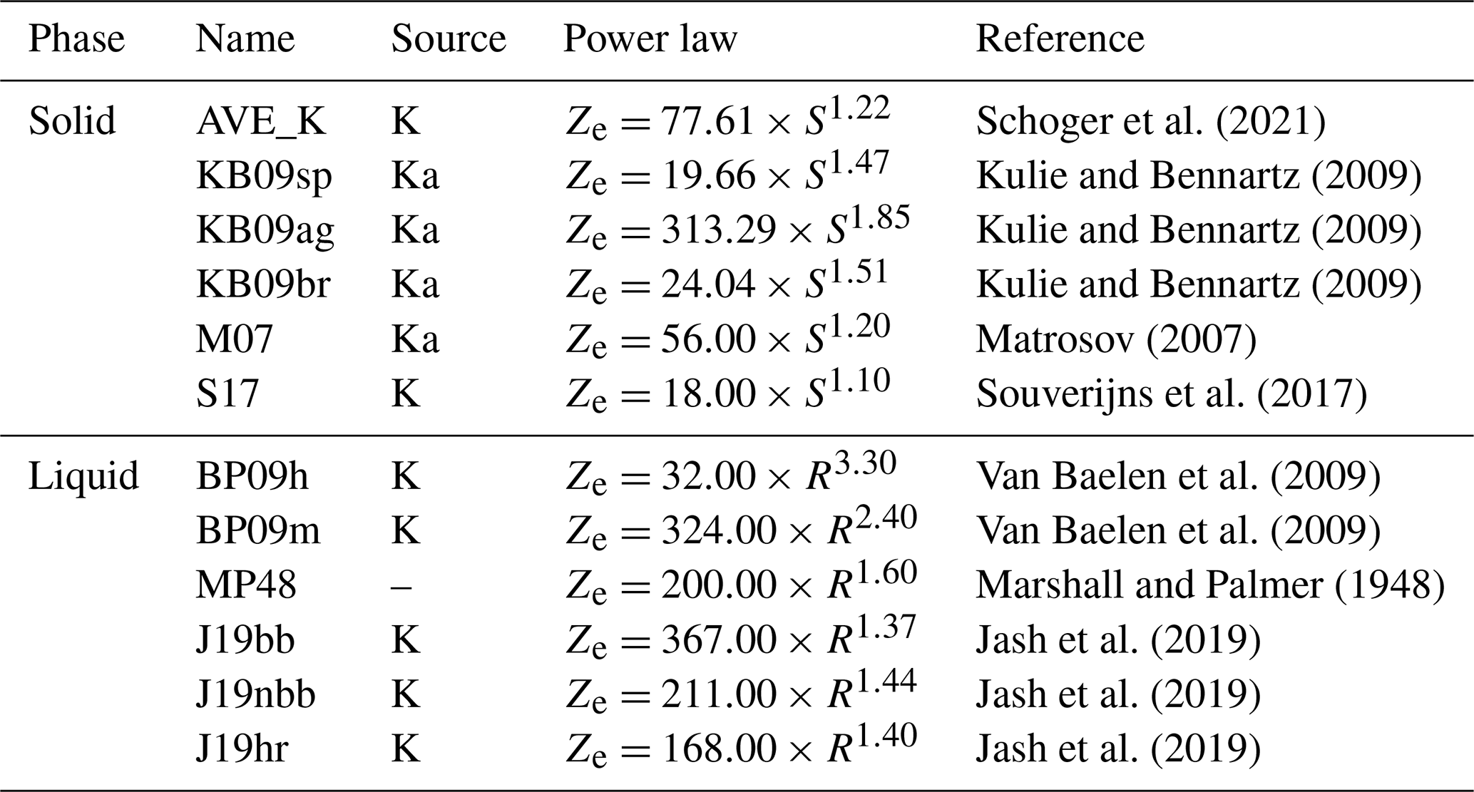
We examine an ensemble of 12 Ka- and K-band relationships in this work to compare with model output from DeepPrecip (Table 2). As a consequence of the short temporal period (20 min) used in this analysis, MSE values are typically small (<0.1 mm2). Each relationship was applied to a near-surface bin in the reflectivity profile (bin 5 for DPfull and DPnear, and bin 11 for DPfar) to derive a corresponding surface precipitation estimate. These bins were selected based on a sensitivity analysis where we examined the performance of multiple near-surface high-importance regions of the vertical column (not shown). The best performing regions were identified as the above bins (5 and 11) based on the respective region of the vertical column being considered (near or far). More information regarding the derivation of each relationship can be found in Table 2.
To further evaluate the performance of DeepPrecip, we also include model comparisons to a set of six site-derived Ze−P (reflectivity precipitation) power law relations. Each Ze−P relationship is empirically derived from the collocated MRR and Pluvio data at each observational site examined in this work (excluding Cold Lake and Ny-Ålesund due to the limited available sample and vertical extent of each site, respectively). Each Ze−P relation is fit via a non-linear least-squares approach for finding optimal a and b coefficients in Eq. (1) using SciPy's curve_fit optimization algorithm (Virtanen et al., 2020). Each Ze−P relationship was then applied to bin 5 reflectivities at each site (i.e. the same process as is used for relationships) and compared with in situ observations to assess their general accuracy.
3.2 Neural network architecture
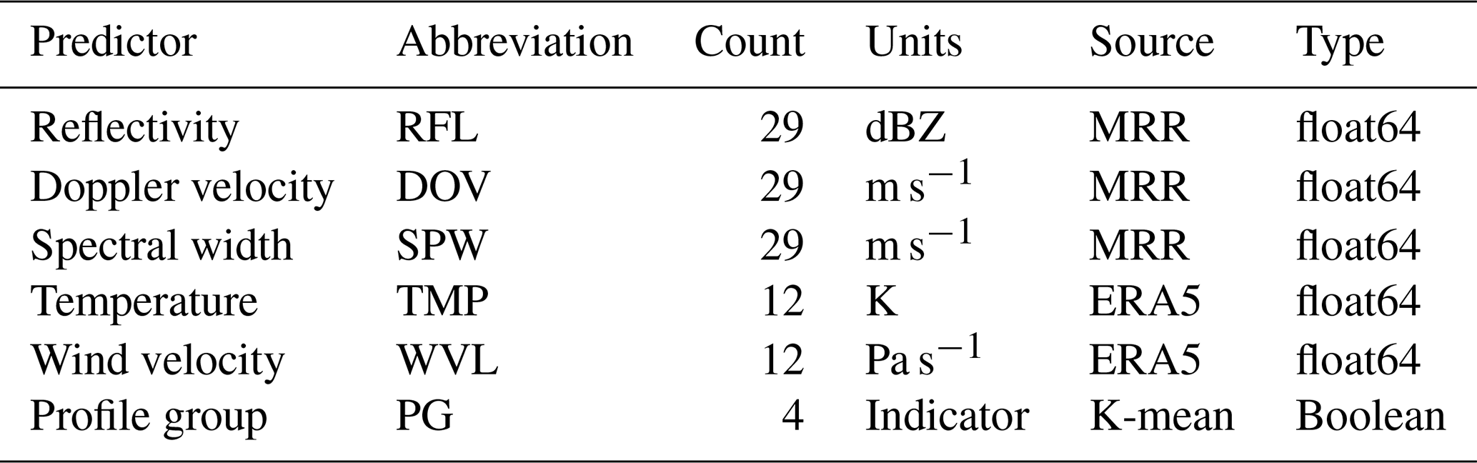
DeepPrecip is a feedforward convolutional neural network that takes as input a vector of 115 atmospheric covariates (Table 3), performs a feature extraction of the vertical column, and outputs a single surface precipitation estimate using a fully connected multilayer perceptron. While the structure of this final version of DeepPrecip is complex, the retrieval evolved from a much simpler initial state based on a multiple linear regression (MLR) model. Due to clear nonlinearities between observed reflectivity data and surface precipitation accumulation, the MLR model was unable to capture in situ variability and provided estimates near the mean accumulation value. Similar radar-based precipitation retrieval studies by H. Chen et al. (2020) and Choubin et al. (2016) demonstrated much better performance using an ML-based approach, which led to the development of a random forest (RF) model, an MLP, and finally the CNN.
Table 3Summary of DeepPrecip full vertical column model input covariates.
The 1D convolutional layers perform a feature extraction of the vertical column of inputs to reduce the total number of parameters being fed into DeepPrecip's fully connected dense layers. This 1D-CNN structure can identify relationships within the vertical column, save on memory, and lower computational training time requirements. To perform a 1D feature extraction, the forward propagation step between the previous convolutional layer (l−1) to the input neurons of the current layer (l) is expressed in Eq. (2) (Abdeljaber et al., 2017):
where k and l refer to the kth neuron for layer l with x as the resulting input and b as the scalar bias. The s and w terms represent the neuron output and kernel weight matrix respectively, from the ith neuron of layer l−1 (and to the kth neuron of layer l for w). The function “f()” represents the activation function used to transform the weighted sum into an output to be used in the following network layer.
The RF model tested in this study was based on previous work from King et al. (2022), where an RF was used to retrieve surface snow accumulation from a collocated X-band and Pluvio2 instrument at a single experiment site (GCPEx). The RF developed in said study demonstrated good skill in estimating surface accumulation, and so we incorporate the same model here (retrained on the MRR and ERA5 data from this study) as a baseline comparison to other ML retrieval methods (i.e. DeepPrecip).
The final DeepPrecip model structure is outlined in Fig. 2b. It includes two 1D-convolutional layers, a 1D max pooling layer, dropout layer, and flattening layer, and concludes in a dense MLP regressor with three hidden layers. The total number of trainable model parameters in DeepPrecip is 3 937 793. Model training and testing was performed using a 90/10 (non-shuffled) split on each site to generate training and testing datasets for each location. As an additional preprocessing step, we standardize all input covariates to remove the mean and by scaling inputs to unit variance. The non-shuffled nature of this splitting process allows for DeepPrecip estimates to be validated against unseen data and prevents overfitting from training on temporally autocorrelated vertical column inputs. Additionally, this stratified selection process guarantees that an equal percentage of data from each site is included during training.
Retrieval accuracy is primarily assessed using a mean squared error (MSE) skill metric calculated between each model's estimated surface accumulation values and the total Pluvio2 non-real-time reference accumulation observations over 20 min. Performance statistics are reported from the average skill of the test portion of a non-shuffled 90/10 train and test CV split (i.e. DeepPrecip trained and tested 10 times on different contiguous portions of the full available sample). Note that each split is stratified to include 10 % of each station's sample in every test split. Uncertainty estimates are calculated by running each CV split 50 times using dropout to gain additional insight into model variability (resulting in 500 total model instances). The dropout layers simulate training a large number of models with differing architectures in a highly parallelized manner by randomly deactivating (or dropping) a certain fraction of nodes within the network to provide a distribution of retrieval estimates.
3.3 Hyperparameter optimization
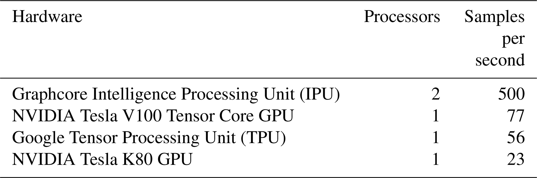
DeepPrecip was developed, trained, and optimized on Graphcore intelligence processing units (IPUs) MK2 Classic IPU-POD4 (Louw and McIntosh-Smith, 2021), which significantly sped up the training time by a factor of 6.5 compared to a state-of-the-art NVIDIA Tesla V100 GPU. Additional training throughput comparisons are included in Table 4. Training was completed using a combination of open-source Python packages including Keras, Tensorflow, and scikit-learn. An extension of stochastic gradient descent known as Adam optimization (adaptive moment estimation) is used to continually update internal network weights in the model during training to minimize a standard MSE loss function (Eq. 3) and track model learning over time:
Table 4DeepPrecip model training throughput comparisons running on Tensorflow (v2.4.3) using a batch size of 128 samples on different hardware. Note that 2 IPUs were used in comparison to 1 GPU/TPU to equalize average computation costs when training DeepPrecip using each piece of hardware.
Hyperparameters do not change value during training (in contrast to model parameters like internal node weights), but they play a critical role in the neural network learning process to map input features to an output. Selecting optimal hyperparameter values is an important part in constructing a model that minimizes loss, improves model efficiency and quality, and mitigates overfitting. Multiple steps were taken to address concerns of model overfitting. In addition to the use of non-shuffled training, we employ multiple regularization methods, including early stopping, dropout, the application of layer weight constraints, and L2 regularization (details in Table 5). L2 regularization (or ridge regression) adds an additional penalty term to the MSE loss function, which helps to create less complex models when dealing with many input features to improve model generalization.
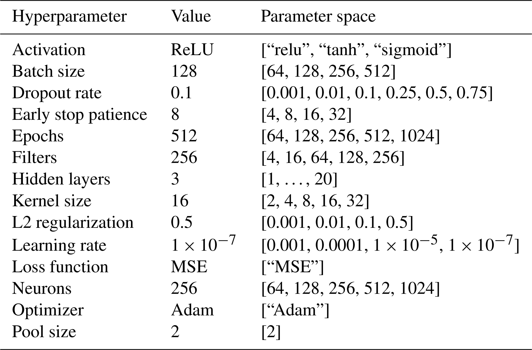
To select the optimal values for the aforementioned hyperparameters, and to optimize DeepPrecip's general structure, we use a form of hyperparameterization known as hyperband optimization (Li et al., 2017). Hyperband is a variation of Bayesian optimization that intelligently samples the parameter space to find hyperparameter values that minimize loss while learning from previous selections. Hyperband adds an additional component to the analysis by also slowly increasing the number of epochs run during each phase of the optimization process to sample in a more efficient manner. DeepPrecip hyperparameters were derived by running a 10-fold CV hyperband optimization continuously on a single Graphcore IPU for approximately 2 weeks. The final hyperparameter values (and their respective parameter search spaces) can be found in Table 5.
3.4 Unsupervised classification layer
An unsupervised k-means clustering preprocessing step is also applied using MRR reflectivity profiles as input to provide DeepPrecip with insights into distinct profile group (PG) vertical column structures (Fig. 2b). Minimizing the within-cluster sum of squares between each vertical column radar estimate results in k=4 PGs being selected using the within-cluster-sum of squared errors of the elbow criterion method (Fig. 3). The elbow method is a clustering heuristic that allows for an optimal number of clusters to be selected as a function of diminishing returns of explained variation (i.e. finding the elbow or “knee of the curve”). K-means clustering was applied using Python's scikit-learn package on all input reflectivity data to generate four profile clusters, which were included as additional input parameters to DeepPrecip. These clusters are useful for partitioning the precipitation data into groups based on different precipitation intensity-classes (trace, low, medium, and high intensity) to identify where DeepPrecip finds the most important contributors to high retrieval accuracy for each category of storm intensity. Derived cluster groups are useful for interpreting feature importances from the model output (Sect. 4.2).
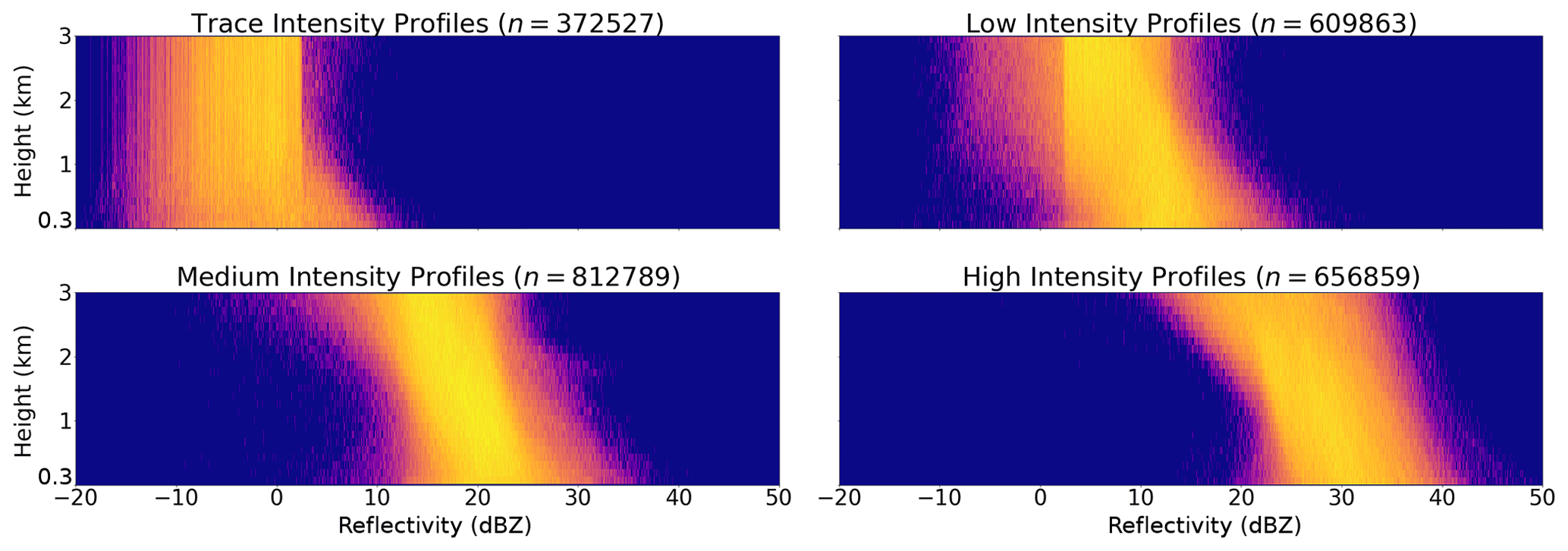
Figure 3K-means cluster reflectivity intensity-classes of vertical profiles from the MRR instruments at all sites. A total of 2 452 038 vertical profiles are organized by reflectivity intensity (dBZ) into k=4 precipitation intensity subsets. The four groups were selected using the within-cluster sum of squared errors of the elbow method.
4.1 DeepPrecip retrieval performance
We first examine the differences in performance between DeepPrecip and an RF that has demonstrated good performance in our previous work (not shown) to assess the capabilities of a less-sophisticated ML-based approach over a CNN. DeepPrecip demonstrates improved skill in capturing most of the peaks and troughs in observed precipitation variability (Fig. 4a). These differences are demonstrated the most clearly in Fig. 4a at OLYMPEx and JOYCE, where DP more accurately predicts Pluvio2 precipitation extremes compared to the RF. Both models appear to struggle in capturing accumulation intensities during periods of mixed-phase precipitation when temperatures are near 0 ∘C (i.e. Marquette, JOYCE, and the tail end of OLYMPEx 1) due to a lack of training data with similar climate conditions and the complex nature of such events. DP does demonstrate improved skill at capturing light intensity precipitation at the beginning of the JOYCE period (compared to the RF); however, this is with some uncertainty as noted by the wider shaded region (one standard deviation). Performance statistics (Fig. 4b) summarize these improvements with DeepPrecip showing MSE values 21 % lower and r2 values 34 % higher (significant at α<0.05) compared to the RF.
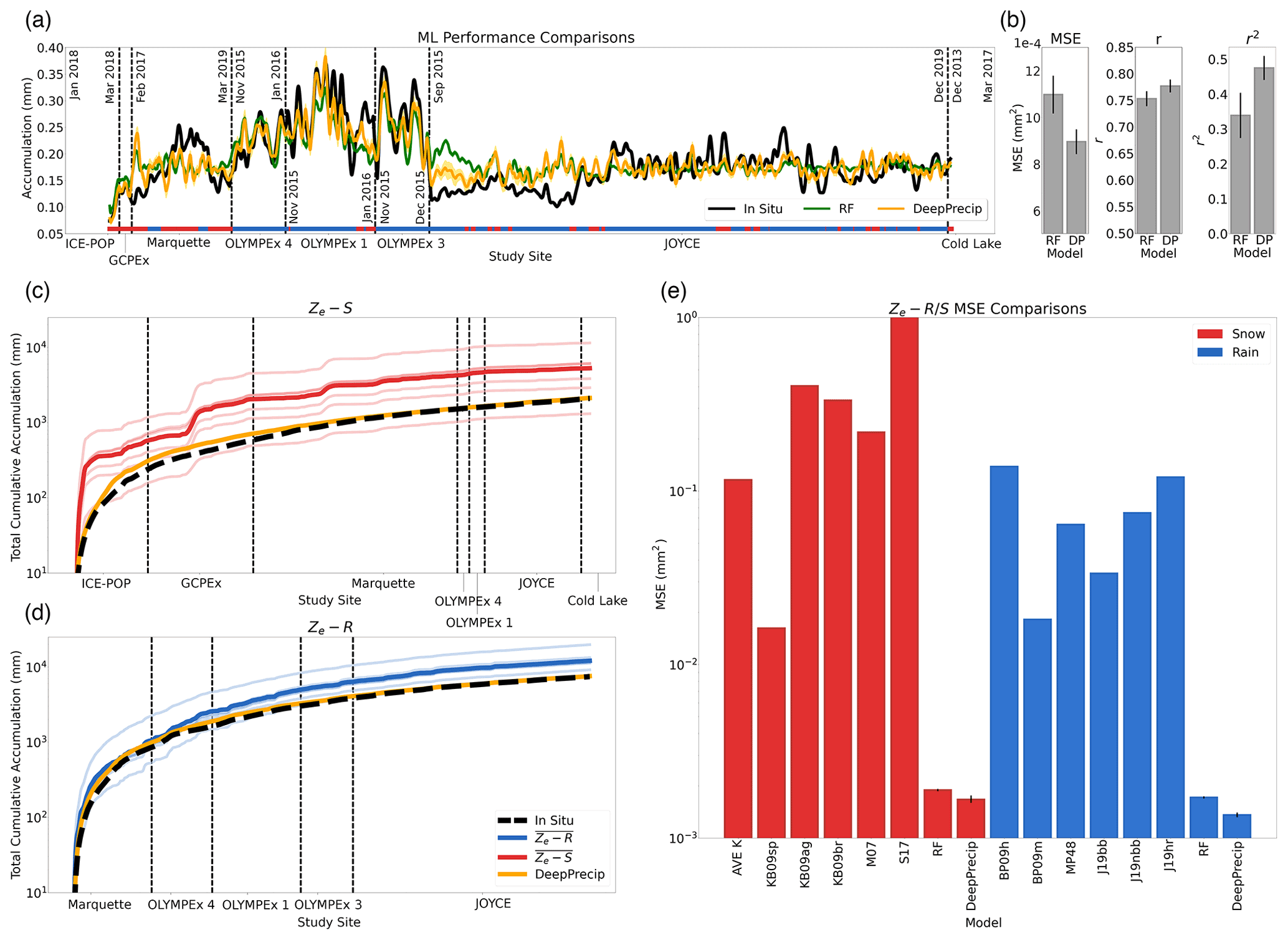
Figure 4Performance comparisons between DeepPrecip (DP), an RF, and an ensemble of power law-derived retrievals of surface precipitation. (a) Running mean (window size 500 time steps) of accumulation for all sites with Pluvio2 measurements in black, RF estimates in green, and DeepPrecip in yellow. Data is sorted by station and then time, with each station separated by a dashed vertical line. One standard deviation from 50 dropout runs per cross-validated instance is shown in the shaded regions (most notable in DP estimates at the start of JOYCE). (b) Performance statistics for RF/DeepPrecip accuracy, including MSE, Pearson correlation (r), and r2 with error bars showing one standard deviation. (c) Time series of total accumulation estimates over the full observation period for all Ze−S relationships (individual light red lines) and DeepPrecip. The mean of the Ze−S relationships is shown in bold. (d) The same as in (c) but for Ze−R. (e) Phase-partitioned log-scale MSE values between each model and in situ observations from 50 model realizations. Note that S17 MSE values extend beyond the top of the graph to 101 mm2.
The total cumulative surface accumulation comparisons between DeepPrecip and each relationship are then examined in Fig. 4c for both rain and snow. To examine model skill across different precipitation phases, a simple temperature threshold is imposed, where retrievals recorded during periods with temperatures below 5 ∘C are classified as snow and periods equal to or warmer than 5 ∘C as rain. DeepPrecip more accurately captures surface precipitation quantities when compared to the estimates, with a total accumulation curve similar in shape to that of in situ observations, indicating that DeepPrecip captures the observed precipitation variability and magnitude more closely. Log-scale MSE statistics are calculated between each model and in situ records in Fig. 4d and indicate that DeepPrecip consistently outperforms traditional power law methods by 200 % on average. As a general precipitation retrieval algorithm, we do not explicitly train a DeepPrecipsnow and DeepPreciprain model for different precipitation phases with unique regional atmospheric microphysical conditions. While the models shown in Fig. 4c and d are bespoke for rain or snow, DeepPrecip is trained on all data with no a priori knowledge of the underlying physical precipitating particle state.
DeepPrecip estimates of accumulated rain display a lower MSE than that of snow (Fig. 4d). We believe these differences to be twofold: (1) the larger sample of rainfall events in the training data (three times that of snowfall); and (2) the more complex nature of snow particle microphysics. Unlike the uniform properties of a rain droplet, the shape, size, and fall speed of solid precipitation is much more dynamic and challenging to model (Wood et al., 2013). Continued issues with interference from wind may have also impacted the accuracy of in situ measurements of snow accumulation, leading to higher uncertainty and error (further discussions on these uncertainties in Sect. 5) (Kochendorfer et al., 2017). To visualize the range in uncertainty from the CNN model estimates, we display confidence intervals showing one standard deviation in Fig. 4b and d from 50 DeepPrecip model realizations using dropout. Both ML-based models exhibit the highest uncertainty during periods of mixed-phase precipitation at GCPEx and Marquette along with high intensity precipitation at OLYMPEx.
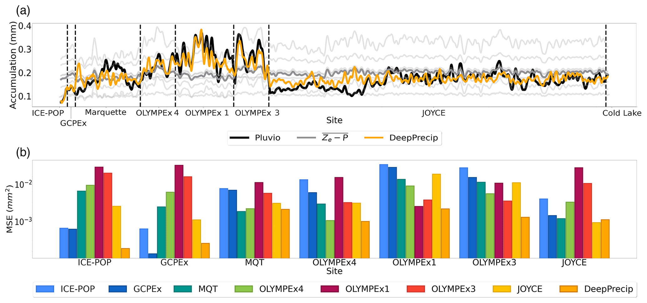
Figure 5Site-derived empirical Ze−P power law performance comparisons. (a) The same as Fig. 4a, except now using Ze−P relationships derived at each study site. (b) MSE values for DeepPrecip and each Ze−P relationship when tested on each site.
To further evaluate DeepPrecip's retrieval skill over traditional methods, we compare model performance to a set of six custom Ze−P site-derived power laws (derivation details in Sect. 3). While Ze−P relationships typically perform well in the regional climate under which they were derived, they do not generalize well outside of said climate. This lack of robustness is visible in the differences between in situ and Ze−P estimates of accumulation in Fig. 5a, where each Ze−P (light gray line) displays consistent positive or negative biases, and no single power law captures the high variability in accumulation across multiple sites. For instance, OLYMPEx 1 and OLYMPEx 3-derived relationships produce a strong positive bias at JOYCE, and the JOYCE-derived Ze−P power law is quite negatively biased when applied at OLYMPEx. The mean of all six custom power laws is shown in bold gray, and while it closely captures total mean accumulation across all sites, it is unable to model the high variability in precipitation intensity.
The resulting MSE from the application of each custom Ze−P relationship to each site (along with DeepPrecip) further demonstrates DeepPrecip's improved robustness (Fig. 5b). In all other cases, DeepPrecip either outperforms all Ze−P power laws or is only slightly worse than the power law derived for the site in which it is being tested. On average, DeepPrecip retrievals result in 160 % lower MSE values than all Ze−P site-derived power laws estimates when applied to the testing data across the full spatiotemporal domain (Table 6). Figure 5b also displays a model intercomparison of each Ze−P relation, where we can clearly see how Ze−P relations like those derived at OLYMPEx 1 and 3 are clearly unable to capture the vastly different snowfall regimes at sites like ICE-POP, GCPEx, and JOYCE with their much larger MSE values for these sites.
Table 6MSE values (in × 10−3 mm2) for all vertical extent experiments across all models for both solid and liquid precipitation.
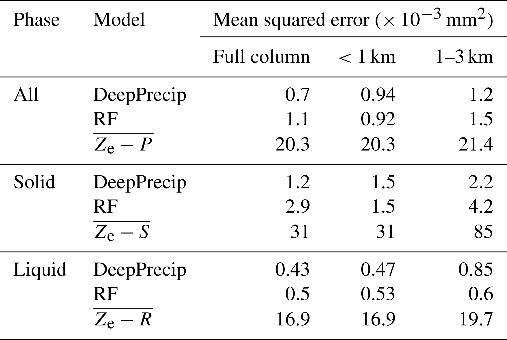
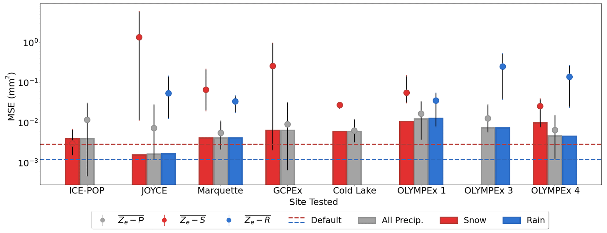
Figure 6Leave-site-out full column DeepPrecip performance robustness analysis. Each bar represents a DeepPrecip full column log-scale MSE value when trained on all precipitation data, excluding the noted site, and then validated against said excluded site (the dashed line is the default DeepPrecip model with all sites). Each red and blue dot represents the average relationship estimate tested in the same manner (error bars represent the min and max ensemble values). Gray dots represent the mean, min, and max ensemble values from all site-derived Ze−P relationships (excluding the relationship derived from site being tested), when applied to each site.
The robustness of DeepPrecip was further evaluated using a leave-one-out cross validation (CV) for each site of training observations. This approach tests the skill of DeepPrecip at predicting precipitation for a location that was not included in the training data, which is a strong indicator of the generalizability of the model. Log-scale MSE results of this test for each site are shown in Fig. 6 for each precipitation-phase subset, along with the corresponding average estimate when applied at that site. These findings demonstrate similar performance to the baseline DeepPrecip model skill, which continues to outperform all traditional power law techniques on average. The large range in skill in the power law relationships at most sites (wide error bars) further demonstrates the relative lack of generalizabiltiy of relationships to different regional climates. Further, the site-derived power law fits (gray dots) perform worse on average than DeepPrecip for locations that are close in proximity (i.e. the OLYMPEx sites).
Predictably, DeepPrecip performance degrades compared to the baseline model when the testing site is left out since the model is no longer trained using data representing the regional climate of the site being tested. This difference in performance is most notable at the set of OLYMPEx sites, and while DeepPrecip performance is still improved over the relationships, we note a substantial percentage increase in MSE (375 % on average) at these locations. OLYMPEx measurements were the only observational datasets without any gauge shielding, which is a likely source of uncertainty further contributing to this increase in error when the site is removed from the training set (Kochendorfer et al., 2022).
4.2 Quantifying sources of retrieval accuracy
Identifying regions within the vertical column that are the most important contributors towards retrieval accuracy is critical for informing future satellite-based radar precipitation retrievals. The ground-based radar instruments used in this work do not suffer from the same ground clutter contamination issues typical of satellite-based radar observations, and we are, therefore, able to quantify the contributions to model skill arising from the included boundary layer reflectivity measurements in DeepPrecip. Separating the training data into three subsets based on vertical extent and generating new models with this data allows us to examine changes in performance as a function of information availability. These subsets include: DPfull (all 29 vertical bins, i.e. the baseline model), DPnear (the lowest 1 km; 8 bins), and DPfar (1–3 km; 21 bins). DeepPrecip MSE results (Table 6) for each subset suggest that the information provided by a combination of both near-surface and far-profile data results in the highest accuracy.
Since Ny-Ålesund MRR observations were recorded with a maximal vertical extent of 1 km, they are only included in DPnear. Model skill when including and excluding Ny-Ålesund training data (19 000 samples) was examined to determine whether it was confounding comparisons between the aforementioned vertical profile subset models. The results of these tests suggested that the impact on overall performance is negligible across both precipitation phases when Ny-Ålesund is included or excluded in the training set.

Figure 7Phase-partitioned surface precipitation accumulation anomaly frequency distributions. DeepPrecip is trained and tested on three subsets of bins from the vertical column: DPnear (<1 km), DPfar (1–3 km), and DPfull (the entire vertical column) for (a) solid and (b) liquid precipitation.
Distributions of surface precipitation anomalies appear distinct for rain and snow (Fig. 7), with the full column model more closely capturing accumulation recorded by in situ gauges. Anomaly frequencies are derived by removing the mean accumulation estimate for each phase at each site. We attribute the structural differences between the anomaly distributions of snow and rain to the more complex particle size distributions (PSDs) of snowfall coupled with the more variable particle water content of snow compared to that of rain (Yu et al., 2020). Additional uncertainties in the surface Pluvio2 measurement gauge observational records of snowfall due to gauge undercatch are another likely contributor of increased error (Kochendorfer et al., 2022). In Fig. 7a, both DPfar and DPnear exhibit higher anomaly values with a flattened curve top and heavy tails. Using a combination of information from both near and far bins reduces these biases and tightens each accumulation anomaly distribution around zero. A similar trend is also present for rain in Fig. 7b, where we again most closely capture the in situ anomaly distribution using DPfull.
A major challenge in deep learning is interpreting model output. SHapley Additive exPlanations (SHAP) (Lundberg and Lee, 2017), is a game theory approach to artificial intelligence model interpretability based on Shapley values that has previously been used to great effect in the geosciences (Maxwell and Shobe, 2022; Li et al., 2022). Shapley values quantify the contributions from all permutations of input features on retrieval accuracy to identify which are the most meaningful. While computationally expensive (with exponential time complexity), this process provides local interpretability within the model by examining how each possible combination of all input features impacts model accuracy (Jia et al., 2020). Here, the calculated Shapley values give insight into the regions of the vertical column that contribute the most useful radar information in the precipitation retrieval.
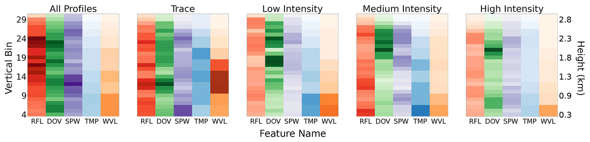
Figure 8Normalized vertical column Shapley global feature importance values (i.e. ). Shapley output values are calculated for different subsets of vertical column reflectivities separated into all profiles, trace intensity, low intensity, medium intensity, and high intensity precipitation events based on a k-means clustering of input data (more in Sect. 3.2). Areas of dark color indicate a high feature importance at that location within the vertical column.
Shapley values for the entire dataset used in DPfull indicate that the most important model predictors comprise a combination of both near-surface and far profile bins (Fig. 8). Reanalysis variable model inputs are generally the least influential, except for the trace precipitation case where low-mid level TMP and WVL bins appear highly important (Fig. 8). In all cases, TMP and WVL decrease in importance as a function of height above the surface. DeepPrecip typically considers MRR-derived bins in the 1.5–2.5 km range as the most important predictors. In non-trace intensity profiles, it is the 2 km region Doppler velocity (DOV) observations that are the dominant contributing predictor. When we consider all profiles, reflectivity (the input to relationships) is not necessarily the dominant feature, and it is a combination of 1.5–2 km profile information from reflectivity, Doppler velocity, and spectral width (SPW) that results in the highest model skill. Combinations of these regions within the vertical column appear to allow DeepPrecip to better understand precipitation events with complex cloud structures that would not necessarily be recognized by conventional relations that primarily rely on information from a small subset of near-surface bins.
DeepPrecip not only demonstrates considerable retrieval accuracy without the need for physical assumptions about hydrometeors or spatiotemporal information but also provides insight into the regions of the vertical column that are the most important for improving predictive accuracy. The results from Sect. 4.2 suggest that while the exact altitudes providing predictive information from the vertical column may shift up or down under different precipitation intensities, there exists a consistent combination of both near-surface and far profile bins that always appear as highly important contributors to model skill. Furthermore, while RFL is typically considered as the most important predictor in radar-based precipitation retrievals (Stephens et al., 2008; Skofronick-Jackson et al., 2015), we find that contributions from RFL, DOV, and SPW provide a near-equal level of importance, with respective average percent contributions to model an output of 30 %, 31 %, and 28 %, while ERA5 TMP and WVL variables have a total combined importance of 10 %.
The combined insights from DeepPrecip's multi-model vertical extent evaluations and feature importance analyses demonstrate a potential to influence current and future remote sensing precipitation retrievals using deep learning. Instruments like CloudSat's Cloud Profiling Radar (CPR), or the Global Precipitation Measurement (GPM) mission's Dual-Frequency Precipitation Radar (DPR) also use active radar systems to perform similar, radar-based precipitation retrievals based on data from vertical column reflectivities (Stephens et al., 2008). While CPR and GPM-derived products use a more sophisticated Bayesian retrieval to the relationships evaluated here, the resulting precipitation estimates are still tightly coupled to a priori physical assumptions of particle shape, size, and fall speed, which are a substantial source of uncertainty (Hiley et al., 2010; Wood et al., 2013). Additionally, the results of this study further support prior inference regarding the existence of regions of high importance in the <1 km (near-surface) region of the vertical column relating to shallow-cumuliform precipitation strongly influencing retrieval accuracy. This is an area that is typically masked in satellite-based products (i.e. the radar “blind-zone”) due to surface clutter contamination and was shown in previous work to likely be a major source of underestimation from missing shallow cumuliform precipitation (Maahn et al., 2014; Bennartz et al., 2019). This work motivates the importance of continued research towards obtaining high-quality, non-cluttered near-surface radar data to use as additional model inputs in future space-based retrievals of precipitation.
DeepPrecip is not without uncertainty and error, which will reduce its accuracy when tested against new data. Uncertainties present in the training data (stemming from the MRR, ERA5, or Pluvio2 observations) will propagate through the model and bias the output estimates (Kochendorfer et al., 2022; Jakubovitz et al., 2019). We have taken steps to mitigate the impact of these uncertainties through multiple data alignment and preprocessing decisions (see Sect. 3 for details); however, precipitation gauge undercatch, wind shielding configurations, MRR attenuation, and differences in site-specific vertical extent cannot be eliminated as contributors of retrieval error. While 60 % of the power laws examined in this work were MRR-derived K-band relationships, the remaining 40 % where either Ka-band or the Marshall-Palmer (MP) Rayleigh relationship. While K and Ka are similar radar frequencies, the differences between the two can bias the resulting precipitation estimate when a Ka-derived power law is applied to K-band data (especially during periods of intense precipitation). Furthermore, while the collection of data from multiple sites provides us with a robust training set under multiple regional climates, due to the unique experimental setups at each site, calibration biases between study locations may further reduce DeepPrecip's skill when applied to new data. As the MRR instrument has a limited 3 km maximum vertical range, we also miss possible precipitation events occurring outside of this region, which may contribute to further surface precipitation underestimation. Internal CNN model uncertainty is likely driven, in part, by a combination of the high variability that is typical of precipitation and the limited sample from nine measurement sites over 8 years, which does not fully capture all different forms of possible precipitation structure and occurrence.
The DeepPrecip example code is fully open-source and available for download and use on the project's public GitHub repository (https://github.com/frasertheking/DeepPrecip, last access: 1 August 2022; https://doi.org/10.5281/zenodo.7221133, King, 2022a). In situ data is freely accessible for download on Zenodo (https://doi.org/10.5281/zenodo.5976046, King, 2022b). ERA5 hourly atmospheric data can be downloaded for free from the Copernicus Climate Change Service (C3S) Climate Data Store (https://doi.org/10.24381/cds.adbb2d47, Hersbach et al., 2018). The MRR and Pluvio data used in this study at OLYMPEx, GCPEx, and ICE-POP were provided by NASA's Global Precipitation Measurement (GPM) Ground Validation program (POC: David B. Wolff, david.b.wolff@nasa.gov). MRR and Pluvio data for the Cold Lake site was provided from ECCC observation sites (POC: Robert Crawford, robert.crawford@ec.gc.ca). JOYCE MRR and Pluvio data was provided by the University of Cologne (POC: Stefan Kneifel, skneifel@meteo.uni-koeln.de). Ny-Ålesund MRR and Pluvio data were provided by the German Alfred Wegener Institute for Polar and Marine Research and the French Polar Institute Paul Emile Victor (POC: Kerstin Ebell, kebell@meteo.uni-koeln.de). Marquette MRR and Pluvio data were provided by the Climate and Space Sciences and Engineering group at the University of Michigan (POC: Claire Pettersen, pettersc@umich.edu).
The project concept is due to FK and GD, data was provided by FK, CP, KE, and LM, the methods were developed by FK, GD, and CGF, the model design is due to FK, the data processing and experiments were performed by FK, the writing of the manuscript was done by FK, and the manuscript was edited by FK, CGF, GD, LM, CP, and KE.
The contact author has declared that none of the authors has any competing interests.
Publisher’s note: Copernicus Publications remains neutral with regard to jurisdictional claims in published maps and institutional affiliations.
We also thank the data suppliers Environment and Climate Change Canada (ECCC), the National Aeronautics and Space Administration (NASA), the Institute for Geophysics and Meteorology (IGM) at the University of Cologne, the Korean Meteorological Administration (KMA), the German Alfred Wegener Institute for Polar and Marine Research (AWI), the French Polar Institute Paul Emile Victor (IPEV), and the Climate and Space Sciences and Engineering group at the University of Michigan. This research would not have been possible without data contributions from David Wolff (DW), Claire Pettersen (CP), and Kerstin Ebell (KE). Finally, we would like to thank Graphcore for providing access to their high performance computing systems for training and optimizing the model.
The JOYCE data was provided by the Cloud and Precipitation Exploration Laboratory (CPEX-LAB, http://cpex-lab.de, last access: 19 January 2022), a competence center within the Geoverbund ABC/J.
This research has been supported by the Natural Sciences and Engineering Research Council of Canada (grant no. 547060), the Canadian Space Agency Earth System Science: Data Analyses fund, and the Deutsche Forschungsgemeinschaft (DFG, German Research Foundation – Project-ID 268020496 – TRR17).
This paper was edited by Gianfranco Vulpiani and reviewed by three anonymous referees.
Abdeljaber, O., Avci, O., Kiranyaz, S., Gabbouj, M., and Inman, D. J.: Real-time vibration-based structural damage detection using one-dimensional convolutional neural networks, J. Sound Vib., 388, 154–170, https://doi.org/10.1016/j.jsv.2016.10.043, 2017. a
Adhikari, A., Ehsani, M. R., Song, Y., and Behrangi, A.: Comparative Assessment of Snowfall Retrieval From Microwave Humidity Sounders Using Machine Learning Methods, Earth and Space Science, 7, e2020EA001357, https://doi.org/10.1029/2020EA001357, 2020. a
Bennartz, R., Fell, F., Pettersen, C., Shupe, M. D., and Schuettemeyer, D.: Spatial and temporal variability of snowfall over Greenland from CloudSat observations, Atmos. Chem. Phys., 19, 8101–8121, https://doi.org/10.5194/acp-19-8101-2019, 2019. a
Boudala, F. S., Gultepe, I., and Milbrandt, J. A.: The Performance of Commonly Used Surface-Based Instruments for Measuring Visibility, Cloud Ceiling, and Humidity at Cold Lake, Alberta, Remote Sens., 13, 5058, https://doi.org/10.3390/rs13245058, 2021. a
Buttle, J. M., Allen, D. M., Caissie, D., Davison, B., Hayashi, M., Peters, D. L., Pomeroy, J. W., Simonovic, S., St-Hilaire, A., and Whitfield, P. H.: Flood processes in Canada: Regional and special aspects, Can. Water Resour. J., 41, 7–30, https://doi.org/10.1080/07011784.2015.1131629, 2016. a
Chen, H., Chandrasekar, V., Cifelli, R., and Xie, P.: A Machine Learning System for Precipitation Estimation Using Satellite and Ground Radar Network Observations, IEEE T. Geosci. Remote, 58, 982–994, https://doi.org/10.1109/TGRS.2019.2942280, 2020. a
Chen, L., Cao, Y., Ma, L., and Zhang, J.: A Deep Learning-Based Methodology for Precipitation Nowcasting With Radar, Earth and Space Science, 7, e2019EA000812, https://doi.org/10.1029/2019EA000812, 2020. a
Choubin, B., Khalighi-Sigaroodi, S., and Malekian, A.: Multiple linear regression, multi-layer perceptron network and adaptive neuro-fuzzy inference system for forecasting precipitation based on large-scale climate signals, Hydrolog. Sci. J., 61, 1001–1009, https://doi.org/10.1080/02626667.2014.966721, 2016. a
Colli, M., Lanza, L. G., La Barbera, P., and Chan, P. W.: Measurement accuracy of weighing and tipping-bucket rainfall intensity gauges under dynamic laboratory testing, Atmos. Res., 144, 186–194, https://doi.org/10.1016/j.atmosres.2013.08.007, 2014. a, b
Ehsani, M. R. and Behrangi, A.: A comparison of correction factors for the systematic gauge-measurement errors to improve the global land precipitation estimate, J. Hydrol., 610, 127884, https://doi.org/10.1016/j.jhydrol.2022.127884, 2022. a
Ehsani, M. R., Behrangi, A., Adhikari, A., Song, Y., Huffman, G. J., Adler, R. F., Bolvin, D. T., and Nelkin, E. J.: Assessment of the Advanced Very High Resolution Radiometer (AVHRR) for Snowfall Retrieval in High Latitudes Using CloudSat and Machine Learning, J. Hydrometeorol., 22, 1591–1608, https://doi.org/10.1175/JHM-D-20-0240.1, 2021. a
Gergel, D. R., Nijssen, B., Abatzoglou, J. T., Lettenmaier, D. P., and Stumbaugh, M. R.: Effects of climate change on snowpack and fire potential in the western USA, Climatic Change, 141, 287–299, https://doi.org/10.1007/s10584-017-1899-y, 2017. a
Hersbach, H., Bell, B., Berrisford, P., Biavati, G., Horányi, A., Muñoz Sabater, J., Nicolas, J., Peubey, C., Radu, R., Rozum, I., Schepers, D., Simmons, A., Soci, C., Dee, D., and Thépaut, J.-N.: ERA5 hourly data on single levels from 1959 to present, Copernicus Climate Change Service (C3S) Climate Data Store (CDS) [data set], https://doi.org/10.24381/cds.adbb2d47, 2018. a
Hersbach, H., Bell, B., Berrisford, P., Hirahara, S., Horanyi, A., Muaoz-Sabater, J., Nicolas, J., Peubey, C., Radu, R., Schepers, D., Simmons, A., Soci, C., Abdalla, S., Abellan, X., Balsamo, G., Bechtold, P., Biavati, G., Bidlot, J., Bonavita, M., De Chiara, G., Dahlgren, P., Dee, D., Diamantakis, M., Dragani, R., Flemming, J., Forbes, R., Fuentes, M., Geer, A., Haimberger, L., Healy, S., Hogan, R. J., Halm, E., Janiskova, M., Keeley, S., Laloyaux, P., Lopez, P., Lupu, C., Radnoti, G., de Rosnay, P., Rozum, I., Vamborg, F., Villaume, S., and Thacpaut, J.-N.: The ERA5 global reanalysis, Q. J. Roy. Meteor. Soc., 146, 1999–2049, https://doi.org/10.1002/qj.3803, 2020. a
Hiley, M. J., Kulie, M. S., and Bennartz, R.: Uncertainty Analysis for CloudSat Snowfall Retrievals, J. Appl. Meteorol. Clim., 50, 399–418, https://doi.org/10.1175/2010JAMC2505.1, 2010. a, b
Houze, R. A., McMurdie, L. A., Petersen, W. A., Schwaller, M. R., Baccus, W., Lundquist, J. D., Mass, C. F., Nijssen, B., Rutledge, S. A., Hudak, D. R., Tanelli, S., Mace, G. G., Poellot, M. R., Lettenmaier, D. P., Zagrodnik, J. P., Rowe, A. K., DeHart, J. C., Madaus, L. E., Barnes, H. C., and Chandrasekar, V.: The Olympic Mountains Experiment (OLYMPEX), B. Am. Meteorol. Soc., 98, 2167–2188, https://doi.org/10.1175/BAMS-D-16-0182.1, 2017. a, b, c
Jakubovitz, D., Giryes, R., and Rodrigues, M. R. D.: Generalization Error in Deep Learning, in: Compressed Sensing and Its Applications: Third International MATHEON Conference 2017, 4–8 December 2017, Berlin, Germany, edited by: Boche, H., Caire, G., Calderbank, R., Kutyniok, G., Mathar, R., and Petersen, P., Springer International Publishing, Cham, 153–193, https://www3.math.tu-berlin.de/numerik/csa2017/index.html (last access: 10 July 2022), 2019. a
Jameson, A. R. and Kostinski, A. B.: Spurious power-law relations among rainfall and radar parameters, Q. J. Roy. Meteor. Soc., 128, 2045–2058, https://doi.org/10.1256/003590002320603520, 2002. a, b
Jash, D., Resmi, E. A., Unnikrishnan, C. K., Sumesh, R. K., Sreekanth, T. S., Sukumar, N., and Ramachandran, K. K.: Variation in rain drop size distribution and rain integral parameters during southwest monsoon over a tropical station: An inter-comparison of disdrometer and Micro Rain Radar, Atmos. Res., 217, 24–36, https://doi.org/10.1016/j.atmosres.2018.10.014, 2019. a, b, c
Jennings, K. S., Winchell, T. S., Livneh, B., and Molotch, N. P.: Spatial variation of the rain–snow temperature threshold across the Northern Hemisphere, Nat. Commun., 9, 1148, https://doi.org/10.1038/s41467-018-03629-7, 2018. a
Jia, R., Dao, D., Wang, B., Hubis, F. A., Hynes, N., Gurel, N. M., Li, B., Zhang, C., Song, D., and Spanos, C.: Towards Efficient Data Valuation Based on the Shapley Value, arXiv [preprint], https://doi.org/10.48550/arXiv.1902.10275, 17 August 2020. a
Kim, H.-U. and Bae, T.-S.: Preliminary Study of Deep Learning-based Precipitation, Journal of the Korean Society of Surveying, Geodesy, Photogrammetry and Cartography, 35, 423–430, https://doi.org/10.7848/ksgpc.2017.35.5.423, 2017. a
Kim, K., Bang, W., Chang, E.-C., Tapiador, F. J., Tsai, C.-L., Jung, E., and Lee, G.: Impact of wind pattern and complex topography on snow microphysics during International Collaborative Experiment for PyeongChang 2018 Olympic and Paralympic winter games (ICE-POP 2018), Atmos. Chem. Phys., 21, 11955–11978, https://doi.org/10.5194/acp-21-11955-2021, 2021. a
King, F.: frasertheking/DeepPrecip: Full Release (v1.0.0), Zenodo [code], https://doi.org/10.5281/zenodo.7221133, 2022a. a
King, F.: DeepPrecip Training Data, Zenodo [data set], https://doi.org/10.5281/zenodo.5976046, 2022b. a
King, F., Duffy, G., and Fletcher, C. G.: A Centimeter Wavelength Snowfall Retrieval Algorithm Using Machine Learning, J. Appl. Meteorol. Clim., 61, 1029–1039, https://doi.org/10.1175/JAMC-D-22-0036.1, 2022. a
Kochendorfer, J., Nitu, R., Wolff, M., Mekis, E., Rasmussen, R., Baker, B., Earle, M. E., Reverdin, A., Wong, K., Smith, C. D., Yang, D., Roulet, Y.-A., Buisan, S., Laine, T., Lee, G., Aceituno, J. L. C., Alastrué, J., Isaksen, K., Meyers, T., Brækkan, R., Landolt, S., Jachcik, A., and Poikonen, A.: Analysis of single-Alter-shielded and unshielded measurements of mixed and solid precipitation from WMO-SPICE, Hydrol. Earth Syst. Sci., 21, 3525–3542, https://doi.org/10.5194/hess-21-3525-2017, 2017. a
Kochendorfer, J., Earle, M., Rasmussen, R., Smith, C., Yang, D., Morin, S., Mekis, E., Buisan, S., Roulet, Y.-A., Landolt, S., Wolff, M., Hoover, J., Thériault, J. M., Lee, G., Baker, B., Nitu, R., Lanza, L., Colli, M., and Meyers, T.: How Well Are We Measuring Snow Post-SPICE?, B. Am. Meteorol. Soc., 103, E370–E388, https://doi.org/10.1175/BAMS-D-20-0228.1, 2022. a, b, c, d
Kulie, M. S. and Bennartz, R.: Utilizing Spaceborne Radars to Retrieve Dry Snowfall, J. Appl. Meteorol. Clim., 48, 2564–2580, https://doi.org/10.1175/2009JAMC2193.1, 2009. a, b, c, d
Kulie, M. S., Pettersen, C., Merrelli, A. J., Wagner, T. J., Wood, N. B., Dutter, M., Beachler, D., Kluber, T., Turner, R., Mateling, M., Lenters, J., Blanken, P., Maahn, M., Spence, C., Kneifel, S., Kucera, P. A., Tokay, A., Bliven, L. F., Wolff, D. B., and Petersen, W. A.: Snowfall in the Northern Great Lakes: Lessons Learned from a Multisensor Observatory, B. Am. Meteorol. Soc., 102, E1317–E1339, https://doi.org/10.1175/BAMS-D-19-0128.1, 2021. a
Lahnert, U., Schween, J. H., Acquistapace, C., Ebell, K., Maahn, M., Barrera-Verdejo, M., Hirsikko, A., Bohn, B., Knaps, A., OConnor, E., Simmer, C., Wahner, A., and Crewell, S.: JOYCE: Jaelich Observatory for Cloud Evolution, B. Am. Meteorol. Soc., 96, 1157–1174, https://doi.org/10.1175/BAMS-D-14-00105.1, 2015. a
Lemonnier, F., Madeleine, J.-B., Claud, C., Genthon, C., Durán-Alarcón, C., Palerme, C., Berne, A., Souverijns, N., van Lipzig, N., Gorodetskaya, I. V., L'Ecuyer, T., and Wood, N.: Evaluation of CloudSat snowfall rate profiles by a comparison with in situ micro-rain radar observations in East Antarctica, The Cryosphere, 13, 943–954, https://doi.org/10.5194/tc-13-943-2019, 2019. a
Levizzani, V., Laviola, S., and Cattani, E.: Detection and Measurement of Snowfall from Space, Remote Sens., 3, 145–166, https://doi.org/10.3390/rs3010145,2011. a, b
Li, L., Jamieson, K., DeSalvo, G., Rostamizadeh, A., and Talwalkar, A.: Hyperband: a novel bandit-based approach to hyperparameter optimization, J. Mach. Learn. Res., 18, 6765–6816, 2017. a
Li, L., Qiao, J., Yu, G., Wang, L., Li, H., Liao, C., and Zhu, Z.: Interpretable tree-based ensemble model for predicting beach water quality, Water Res., 211, 118078, https://doi.org/10.1016/j.watres.2022.118078, 2022. a
Liu, G.: Deriving snow cloud characteristics from CloudSat observations, J. Geophys. Res.-Atmos., 113, D00A09, https://doi.org/10.1029/2007JD009766, 2008. a, b
Louw, T. and McIntosh-Smith, S.: Using the Graphcore IPU for Traditional HPC Applications, AccML, 4896, EasyChair, https://easychair.org/publications/preprint/ztfj (last access: 10 June 2022), 2021. a
Lundberg, S. M. and Lee, S.-I.: A unified approach to interpreting model predictions, in: Proceedings of the 31st International Conference on Neural Information Processing Systems, NIPS'17, 4–9 December 2017, Long Beach, California, USA, Curran Associates Inc., Red Hook, NY, USA, 4768–4777, ISBN 978-1-5108-6096-4, 2017. a, b
Maahn, M. and Kollias, P.: Improved Micro Rain Radar snow measurements using Doppler spectra post-processing, Atmos. Meas. Tech., 5, 2661–2673, https://doi.org/10.5194/amt-5-2661-2012, 2012. a
Maahn, M., Burgard, C., Crewell, S., Gorodetskaya, I. V., Kneifel, S., Lhermitte, S., Van Tricht, K., and van Lipzig, N. P. M.: How does the spaceborne radar blind zone affect derived surface snowfall statistics in polar regions?, J. Geophys. Res.-Atmos., 119, 13604–13620, https://doi.org/10.1002/2014JD022079, 2014. a
Marshall, J. S. and Palmer, W. M. K.: The Distribution Of Raindrops With Size, J. Atmos. Sci., 5, 165–166, https://doi.org/10.1175/1520-0469(1948)005<0165:TDORWS>2.0.CO;2, 1948. a
Matrosov, S. Y.: Modeling Backscatter Properties of Snowfall at Millimeter Wavelengths, J. Atmos. Sci., 64, 1727–1736, https://doi.org/10.1175/JAS3904.1, 2007. a
Matrosov, S. Y., Shupe, M. D., and Djalalova, I. V.: Snowfall Retrievals Using Millimeter-Wavelength Cloud Radars, J. Appl. Meteorol. Clim., 47, 769–777, https://doi.org/10.1175/2007JAMC1768.1, 2008. a, b
Maxwell, A. and Shobe, C.: Land-surface parameters for spatial predictive mapping and modeling, Earth-Sci. Rev., 226, 103944, https://doi.org/10.1016/j.earscirev.2022.103944, 2022. a
Munchak, S. J., Schrom, R. S., Helms, C. N., and Tokay, A.: Snow microphysical retrieval from the NASA D3R radar during ICE-POP 2018, Atmos. Meas. Tech., 15, 1439–1464, https://doi.org/10.5194/amt-15-1439-2022, 2022. a
Pettersen, C., Kulie, M. S., Bliven, L. F., Merrelli, A. J., Petersen, W. A., Wagner, T. J., Wolff, D. B., and Wood, N. B.: A Composite Analysis of Snowfall Modes from Four Winter Seasons in Marquette, Michigan, J. Appl. Meteorol. Clim., 59, 103–124, https://doi.org/10.1175/JAMC-D-19-0099.1, 2020. a
Quirita, V. A. A., da Costa, G. A. O. P., Happ, P. N., Feitosa, R. Q., Ferreira, R. d. S., Oliveira, D. A. B., and Plaza, A.: A New Cloud Computing Architecture for the Classification of Remote Sensing Data, IEEE J. Sel. Top. Appl., 10, 409–416, https://doi.org/10.1109/JSTARS.2016.2603120, 2017. a
Rasmussen, R., Baker, B., Kochendorfer, J., Meyers, T., Landolt, S., Fischer, A. P., Black, J., Thériault, J. M., Kucera, P., Gochis, D., Smith, C., Nitu, R., Hall, M., Ikeda, K., and Gutmann, E.: How Well Are We Measuring Snow: The NOAA/FAA/NCAR Winter Precipitation Test Bed, B. Am. Meteorol. Soc., 93, 811–829, https://doi.org/10.1175/BAMS-D-11-00052.1, 2012. a, b
Schoger, S. Y., Moisseev, D., Lerber, A. V., Crewell, S., and Ebell, K.: Snowfall-Rate Retrieval for K- and W-Band Radar Measurements Designed in Hyyti, Finland, and Tested at Ny-Alesund, Svalbard, Norway, J. Appl. Meteorol. Clim., 60, 273–289, https://doi.org/10.1175/JAMC-D-20-0095.1, 2021. a, b, c, d
Shi, X., Gao, Z., Lausen, L., Wang, H., Yeung, D.-Y., Wong, W.-K., and Woo, W.-C.: Deep Learning for Precipitation Nowcasting: A Benchmark and A New Model, NeurIPS, arXiv [preprint], https://doi.org/10.48550/arXiv.1706.03458, 12 June 2017. a
Sims, E. M. and Liu, G.: A Parameterization of the Probability of Snow–Rain Transition, J. Hydrometeorol., 16, 1466–1477, https://doi.org/10.1175/JHM-D-14-0211.1, 2015. a
Skofronick-Jackson, G., Hudak, D., Petersen, W., Nesbitt, S. W., Chandrasekar, V., Durden, S., Gleicher, K. J., Huang, G.-J., Joe, P., Kollias, P., Reed, K. A., Schwaller, M. R., Stewart, R., Tanelli, S., Tokay, A., Wang, J. R., and Wolde, M.: Global Precipitation Measurement Cold Season Precipitation Experiment (GCPEX): For Measurement Sake Let It Snow, B. Am. Meteorol. Soc., 96, 1719–1741, https://doi.org/10.1175/BAMS-D-13-00262.1, 2015. a, b
Skofronick-Jackson, G., Petersen, W. A., Berg, W., Kidd, C., Stocker, E. F., Kirschbaum, D. B., Kakar, R., Braun, S. A., Huffman, G. J., Iguchi, T., Kirstetter, P. E., Kummerow, C., Meneghini, R., Oki, R., Olson, W. S., Takayabu, Y. N., Furukawa, K., and Wilheit, T.: The Global Precipitation Measurement (GPM) Mission for Science and Society, B. Am. Meteorol. Soc., 98, 1679–1695, https://doi.org/10.1175/BAMS-D-15-00306.1, 2017. a
Souverijns, N., Gossart, A., Lhermitte, S., Gorodetskaya, I. V., Kneifel, S., Maahn, M., Bliven, F. L., and van Lipzig, N. P. M.: Estimating radar reflectivity – Snowfall rate relationships and their uncertainties over Antarctica by combining disdrometer and radar observations, Atmos. Res., 196, 211–223, https://doi.org/10.1016/j.atmosres.2017.06.001, 2017. a
Stephens, G. L., Vane, D. G., Tanelli, S., Im, E., Durden, S., Rokey, M., Reinke, D., Partain, P., Mace, G. G., Austin, R., L'Ecuyer, T., Haynes, J., Lebsock, M., Suzuki, K., Waliser, D., Wu, D., Kay, J., Gettelman, A., Wang, Z., and Marchand, R.: CloudSat mission: Performance and early science after the first year of operation, J. Geophys. Res.-Atmos., 113, D00A18, https://doi.org/10.1029/2008JD009982, 2008. a, b
Van Baelen, J., Tridon, F., and Pointin, Y.: Simultaneous X-band and K-band study of precipitation to derive specific ZR relationships, Atmos. Res., 94, 596–605, https://doi.org/10.1016/j.atmosres.2009.04.003, 2009. a, b
Virtanen, P., Gommers, R., Oliphant, T. E., Haberland, M., Reddy, T., Cournapeau, D., Burovski, E., Peterson, P., Weckesser, W., Bright, J., van der Walt, S. J., Brett, M., Wilson, J., Millman, K. J., Mayorov, N., Nelson, A. R. J., Jones, E., Kern, R., Larson, E., Carey, C. J., Polat, İ., Feng, Y., Moore, E. W., VanderPlas, J., Laxalde, D., Perktold, J., Cimrman, R., Henriksen, I., Quintero, E. A., Harris, C. R., Archibald, A. M., Ribeiro, A. H., Pedregosa, F., van Mulbregt, P., and SciPy 1.0 Contributors: SciPy 1.0: Fundamental Algorithms for Scientific Computing in Python, Nat. Methods, 17, 261–272, https://doi.org/10.1038/s41592-019-0686-2, 2020. a
Wood, N. B., L'Ecuyer, T. S., Bliven, F. L., and Stephens, G. L.: Characterization of video disdrometer uncertainties and impacts on estimates of snowfall rate and radar reflectivity, Atmos. Meas. Tech., 6, 3635–3648, https://doi.org/10.5194/amt-6-3635-2013, 2013. a, b
Xiao, R., Chandrasekar, V., and Liu, H.: Development of a neural network based algorithm for radar snowfall estimation, IEEE T. Geosci. Remote, 36, 716–724, https://doi.org/10.1109/36.673664, 1998. a
Yang, D.: Double Fence Intercomparison Reference (DFIR) vs. Bush Gauge for “true” snowfall measurement, J. Hydrol., 509, 94–100, https://doi.org/10.1016/j.jhydrol.2013.08.052, 2014. a
Yu, T., Chandrasekar, V., Xiao, H., and Joshil, S. S.: Characteristics of Snow Particle Size Distribution in the PyeongChang Region of South Korea, Atmosphere, 11, 1093, https://doi.org/10.3390/atmos11101093, 2020. a