the Creative Commons Attribution 4.0 License.
the Creative Commons Attribution 4.0 License.
 | 11 Nov 2022
Retrieval of ice water path from the Microwave Humidity Sounder (MWHS) aboard FengYun-3B (FY-3B) satellite polarimetric measurements based on a deep neural network
Wenyu Wang
Zhenzhan Wang
Qiurui He
Lanjie Zhang
The ice water path (IWP) is an important cloud parameter in atmospheric radiation, and there are still great difficulties in its retrieval. Artificial neural networks have become a popular method in atmospheric remote sensing in recent years. This study presents a global IWP retrieval based on deep neural networks using the measurements from the Microwave Humidity Sounder (MWHS) aboard the FengYun-3B (FY-3B) satellite. Since FY-3B/MWHS has quasi-polarization channels at 150 GHz, the effect of the polarimetric radiance difference (PD) was also studied. A retrieval database was established using collocations between MWHS and CloudSat 2C-ICE (CloudSat and CALIPSO Ice Cloud Property Product). Then, two types of networks were trained for cloud scene filtering and IWP retrieval. For the cloud filtering network, the microwave channels show a capacity with a false alarm ratio (FAR) of 0.31 and a probability of detection (POD) of 0.61. For the IWP retrieval network, different combination inputs of auxiliaries and channels were compared. The results show that the five MWHS channels combined with scan angle, latitude, and the ocean/land mask of inputs of auxiliary variables perform best. Applying the cloud filtering network and IWP retrieval network, the final root mean squared error (RMSE) is 916.76 g m−2, the mean absolute percentage error (MAPE) is 92 %, and the correlation coefficient (CC) is 0.65. Then, a tropical cyclone case measured simultaneously by MWHS and CloudSat was chosen to test the performance of the networks, and the result shows a good correlation (0.73) with 2C-ICE. Finally, the global annual mean IWP of MWHS is very close to that of 2C-ICE, and the 150 GHz channels give a significant improvement in the midlatitudes compared to using only 183 GHz channels.
- Article
(12234 KB) - Full-text XML
- BibTeX
- EndNote


Ice clouds play an important role in the global climate (Liou, 1986), and their distribution strongly affects precipitation and the water cycle (Eliasson et al., 2011; Field and Heymsfield, 2015). Long time series and global observations of ice clouds are essential for understanding the Earth's climate system. Depending on the wavelength of observation, satellite remote sensing can measure different cloud microphysics. Microwave measurements can penetrate deeper into cloud layers to measure thick and dense ice clouds, while infrared and visible instruments are mainly used for thin cloud measurements around cloud tops (Liu and Curry, 1998; Weng and Grody, 2000; Stubenrauch et al., 2013). Although the ice water path (IWP) obtained from different instruments shows several differences (Stephens and Kummerow, 2007; Wu et al., 2009), it is of great importance to use remote sensing to determine the bulk and microphysical properties of clouds. Active observations such as lidar and radar and passive measurements such as visible/infrared imaging spectrometers and microwave radiometers have been used to produce cloud products (King et al., 1998; Austin et al., 2009; Delanoë and Hogan, 2010; Deng et al., 2010; Boukabara et al., 2011). Millimetre-frequency radiometers are sensitive to larger precipitating hydrometeors, while sub-millimetre frequencies are sensitive to smaller ice particles (Buehler et al., 2007). Cloud radar has the advantage of higher vertical resolution and sensitivity than passive radiometers and can determine the vertical structure of ice clouds. However, this usually comes at the cost of a low spectral range and low spatial coverage of the observations (Pfreundschuh et al., 2020).
The brightness temperature (TB) depression caused by the scattering of ice particles is usually proportional to the IWP, which simplifies the retrieval method from radiometric measurements (Liu and Curry, 2000). Studies on ice cloud retrieval using radiometers such as the Advanced Microwave Sounding Unit (AMSU), Special Sensor Microwave Imager/Sounder (SSMIS), Microwave Humidity Sounder (MHS), and MicroWave Humidity Sounder (MWHS), as well as limb sounders such as the Microwave Limb Sounder (MLS), Sub-Millimetre Radiometer (SMR), and Superconducting Submillimeter-Wave Limb Emission Sounder (SMILES), have been published for years (Zhao and Weng, 2002; Eriksson et al., 2007; Wu et al., 2008; Sun and Weng, 2012; Millán et al., 2013; Wang et al., 2014). However, these spaceborne radiometers lack the ability to conduct polarization measurement, while dual-polarization measurements above 100 GHz show obvious polarized scattering signals of ice clouds. Recent theoretical model research indicates that the nonspherical and oriented ice particles are the main reason for the polarization signal (Brath et al., 2020).
With increasing frequency, polarimetric measurements will lead to a new understanding of clouds and their microphysical properties (Buehler et al., 2012; Eriksson et al., 2018; Coy et al., 2020; Fox, 2020). Most passive microwave sensors that have dual-polarization channels are limited to frequencies below 100 GHz. However, these sensors are strongly affected by surface contamination. Currently, only the Global Precipitation Measurement Microwave Imager (GPM/GMI) and Microwave Analysis and Detection of Rain and Atmospheric Structures (MADRAS) have observed polarimetric signals from ice clouds above 100 GHz (Defer et al., 2014; Gong and Wu, 2017). By analysing the polarization differences between the 89 and 166 GHz channels of the GMI, Gong and Wu (2017) found that large polarization occurs mainly near convective outflow regions (anvil or stratified precipitation), while in the inner deep convective core and distant cirrus regions, the polarization signal is smaller. It is roughly estimated that neglecting the polarimetric signal in the IWP retrieval will lead to errors of up to 30 % (Gong et al., 2018). Their study further showed that the main source of the 166 GHz high polarimetric radiance difference (PD) is horizontally oriented snow aggregates or large snow particles, while the low polarization signal could be small cloud ice, randomly oriented snow aggregates, foggy snow, or supercooled water (Gong et al., 2020). The Ice Cloud Imager (ICI) will provide a more comprehensive observation of ice clouds. By covering 176 to 668 GHz, ICI has good sensitivity to both large and small ice particles, and its dual-polarization channels also allow the observation of horizontal particles (Eriksson et al., 2020).
The Microwave Humidity Sounder (MWHS) aboard the FengYun-3B (FY-3B) satellite has been proven to provide information about IWP (He and Zhang, 2016). It has quasi-polarization channels at 150 GHz that can provide polarization signals from ice clouds. The neural network is an easy way to find the nonlinear relationship between TB and IWP, while the only problem is the lack of true IWP values. CloudSat is recognized as a relatively accurate instrument for cloud measurement, and its official Level 2C product (2C-ICE) was used in this paper. Numerous studies have been conducted to compare CloudSat products with in situ measurements, and the results show that the Level 2C product is quite reliable when using a combination of Cloud Profiling Radar (CPR) and lidar. Its ice cloud water content (IWC) is fairly close to the in situ observations (Deng et al., 2013; Heymsfield et al., 2017). Although CloudSat products still have considerable uncertainties (Duncan and Eriksson, 2018), they can provide a relatively accurate reference for IWP and IWC. Holl et al. (2010, 2014) present an IWP product (SPARE-ICE) that uses collocations between MHS, AVHRR (Advanced Very High Resolution Radiometer), and CloudSat to train a pair of artificial neural networks. The 89 and 150 GHz channels were excluded, since they are surface sensitive. However, the 150 GHz channel shows good sensitivity to precipitation-sized ice particles (Bennartz and Bauer, 2003). Brath et al. (2018) retrieved IWPs from airborne radiometers of ISMAR (International Submillimetre Airborne Radiometer) and MARSS (Microwave Airborne Radiometer Scanning System) using neural networks.
In this study, we present an analysis of IWP retrieval from the FY-3B/MWHS observations based on deep neural networks. Both TB of 150 GHz (QV and QH) channels and their PD were investigated. First, we collocated the MWHS measurements with the CloudSat/2C-ICE IWP according to the observation time and geolocation. Second, we trained deep neural networks (DNNs) that were used to filter cloud scenes and retrieve the IWP. The effects of different channels (including PD) and auxiliary information on DNN retrieval were also discussed. Finally, the performance of the final configuration networks was evaluated. The trained neural networks were used to retrieve IWP in a tropical cyclone case and the global annual mean IWP map. The zonal mean IWP of MWHS was also compared with Aqua/MODIS, 2C-ICE, and ERA5 reanalysis data. The main aim of this study is to analyse the ability of MWHS in IWP retrieval, especially the role played by the 150 GHz dual-polarization channels.
This paper is organized to describe the data analysis in Sect. 2, followed by the retrieval method in Sect. 3. The IWP retrieval results and analysis are discussed in Sect. 4.1 and 4.2. The network application on tropical cyclones and the global mean maps are shown in Sect. 4.3, with conclusions in Sect. 5.
2.1 Instruments
2.1.1 FY-3B/MWHS
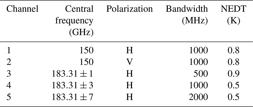
The FY-3B satellite was launched on 5 November 2010, and the MWHS was equipped as one of the main payloads. The MWHS performs the cross-track scanning along the orbit at an angle of ±53.35∘ from nadir to make 98 nominal measurements per scan line, which corresponds to a scan swath of 2645 km in 2.667 s with a resolution of 15 km at nadir. It measures at frequencies from 150 to 190 GHz (two window channels at 150 GHz and three channels near the water vapour absorption line at 183 GHz); these channels are labelled CH.1 to CH.5 hereafter. The details of each channel are shown in Table 1 (Wang et al., 2013). Compared to its successors (i.e. MWHS-II) aboard the FY-3C/D/E satellite, the 150 GHz channels of MWHS have quasi-horizontal and quasi-vertical polarization that can include unique ice cloud information. These channels can provide information near the Earth's surface and lower atmosphere and can also be used to measure atmospheric cloud parameters. For the 150 GHz channels, Zou et al. (2014) investigated the polarization information and concluded that the polarization signal is related to the scan angle and information such as surface wind speed and wind direction and can also be strongly scattered by non-spherical ice cloud particles. Under all weather conditions, except heavy precipitation, all five channels of MWHS can observe water vapour and ice clouds in the atmosphere. In this study, the Level 1B brightness temperature data of MWHS are used.
Table 1Channel characteristics of the MWHS. Note: NEDT is noise equivalent delta temperature.
2.1.2 CloudSat/CALIPSO
CloudSat is a cloud observation satellite that was launched into the NASA A-Train in April 2006, with a 94 GHz cloud profiling radar (CPR) providing continuous cloud profile information (Stephens et al., 2008). The footprint size of the CPR observation is approximately 1.3 km × 1.7 km, with a vertical resolution of 240 m. The scan time for each profile is approximately 0.16 s, and its sensitivity is −30 dBZ. It has an orbital inclination of 98.26∘, which is similar to that of the FY-3B satellite. The Cloud-Aerosol Lidar and Infrared Pathfinder Satellite Observations (CALIPSO) was launched with the CloudSat satellite and designed to fly close to each other in the A-Train satellite constellation to make synergistic observations. The Cloud-Aerosol Lidar with Orthogonal Polarization (CALIOP) carried on the CALIPSO is a dual-wavelength polarized lidar, providing 532 and 1064 nm backscatter profiles with a footprint of 75 m cross-track and 1 km along-track (Winker et al., 2009).
The CloudSat and CALIPSO Ice Cloud Property Product (2C-ICE) contains retrieved estimates of IWC, effective radius, and extinction coefficient for identified ice clouds measured by CPR and CALIOP with orthogonal polarization. The 2C-ICE cloud product uses a combined input of the radar reflectivity factor measured by the CPR and the attenuated backscatter coefficient measured by the lidar at 532 nm to constrain the ice cloud retrieval more tightly than using only the radar product and to produce more accurate results (Mace and Deng, 2019). The combination of CPR and CALIOP provides a more complete measurement of ice clouds than any other current spaceborne sensor measurements. Further study showed that this combined retrieval method is less sensitive to the changes in the assumed microphysical properties than CPR or CALIOP single retrieval (Delanoë and Hogan, 2010).
The 2C-ICE retrieval relies on forward model assumptions. Lidar is sensitive to small particles near the top of the cloud but cannot measure those deep in the cloud, which can lead to an unquantifiable error (Mace et al., 2009). A sensitivity study shows that multiple scattering, assumptions regarding particle habits, and size distribution shapes are critical to the accuracy of the retrieval (Deng et al., 2010). The research also finds that the ratio between the IWC product and in situ measurements is similar to the ratio between two independent in situ measurements (approximately a factor of 2) and concludes that the retrieval agrees well with the in situ data. Since 2C-ICE is used to train the retrieval network in this work, the trained network directly inherits all the systematic errors and limitations of the product.
2.2 Collocation
Collocated measurement is the occurrence where two or more sensors observe the same regions at the same time. One factor for the collocation window requirements is the specific observation target. Ice clouds are a fast-changing (minutes to hours) atmospheric phenomenon that requires a window of short time and small space. Another considered factor in defining the collocation window is the number of meaningful statistics for training.
The ascending node time of CloudSat is between 13:30 and 13:45 at local solar time (LST), which is close to that of FY-3B (13:30 LST). Because of the close orbits and the ascending time between FY-3B and CloudSat, the number of collocated measurements is large. In this study, a collocation dataset of MWHS and 2C-ICE was created by setting the collocation window to 15 min in time and 15 km in space. Since the footprint of MWHS is an order of magnitude larger than that of CPR, multiple 2C-ICE pixels can be found within 1 MWHS pixel. Therefore, the IWP values of 2C-ICE within a circular window (a radius of 7.5 km) were averaged to represent the mean IWP for the MWHS measurement pixel. According to this collocation strategy, 1 207 731 collocations were found between the FY-3B/MWHS and the CloudSat/2C-ICE for 2014. Due to the different observation methods (scan angle and footprint size) of MWHS and CPR/CALIOP, only 14 pixels of 2C-ICE were contained in the best-case collocations (see Fig. 1a). Therefore, the CloudSat footprints cover at most 13.75 % of the area of an MWHS footprint, an error from imprecise collocation was unavoidable, and the representation of the dataset must be considered.
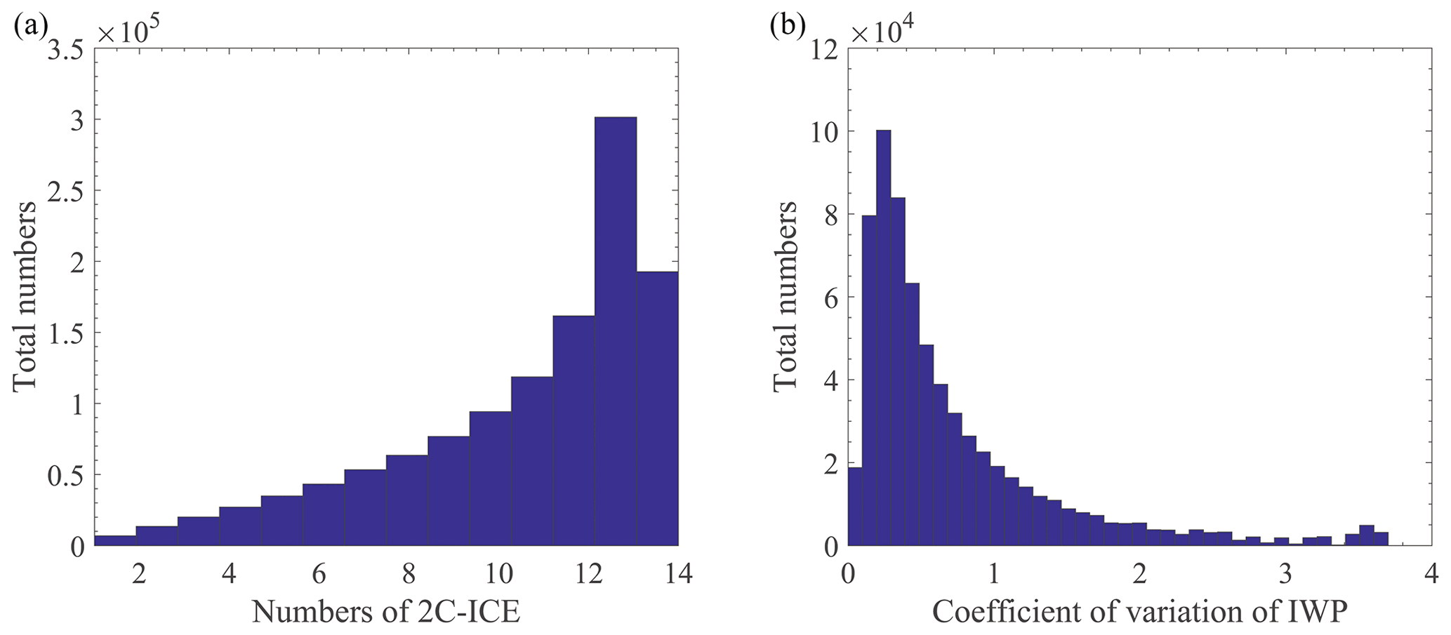
Figure 1Statistical information of MWHS and 2C-ICE collocations in 2014. (a) Histogram of the number of 2C-ICE pixels within an MWHS pixel. (b) Histogram of the coefficient of variation in IWP in collocations.
Figure 1 illustrates the statistics of the 2C-ICE pixels within the MWHS footprints in the collocations. In most cases, more than 10 pixels of 2C-ICE were averaged in the corresponding MWHS pixel. However, there were still many MWHS pixels that covered only a small quantity of 2C-ICE pixels, which means that collocations were poorly represented. The coefficient of variation in each collocation pixel is shown in Fig. 1b. The coefficient of variation was used to represent the IWP dispersion of 2C-ICE pixels in each MWHS pixel. When the coefficient of variation is small, it means that the IWP of 2C-ICE pixels averaged in this MWHS pixel are homogeneous and represent a scene which MWHS observed relatively well. Since the collocation error cannot be estimated, the criteria discussed in Holl et al. (2010) was applied to reduce the sampling effect of collocations. In this study, an MWHS pixel with more than 10 pixels of 2C-ICE and less than 0.6 coefficients of variation was selected for subsequent processing. However, in the case of highly inhomogeneous clouds existing outside the CloudSat field of view, larger uncertainty for the IWP within MWHS pixels cannot be eliminated. After the reduction in inhomogeneous collocations, 665 519 collocations were retained.
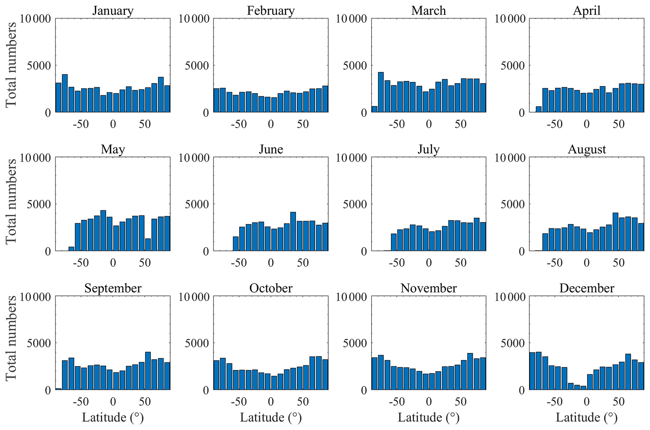
Figures 2 and 3 give statistical information on the scan angle, latitude, and month of the MWHS measurements in this dataset. Since the dataset was used for global retrieval, it must have sufficient samples, and their distribution must represent the real world. According to the statistical results of the collocated MWHS pixels shown in Fig. 2, most of the collocations occurred on one side of the flight direction (from the 40th to the 90th scan pixel). In terms of observation latitude, the collocations near the nadir scan (the 49th pixel) cover the latitude from 80∘ S to 80∘ N, while at the edge of the observation (the 90th pixel), they only cover the tropical regions. In terms of observation time and latitude, Fig. 3 illustrates that there is an obvious lack of data above 60∘ S from April to September, and there are also limited data between 0∘ and 30∘ S in December. The data distribution suggested that the training in polar regions may be inadequate. Due to the high number of collocations near the poles, 121 500 observations at high latitudes were randomly excluded to obtain a balanced dataset. For IWP retrieval, collocations should be classified into two bins (clear-sky scene and cloudy scene), according to a specific IWP threshold. A threshold of IWP >100 g m−2 was preliminarily selected to classify cloudy scenes. Therefore, 81 490 collocations were recognized as cloudy scenes and 462 529 collocations were clear-sky scenes in this dataset.
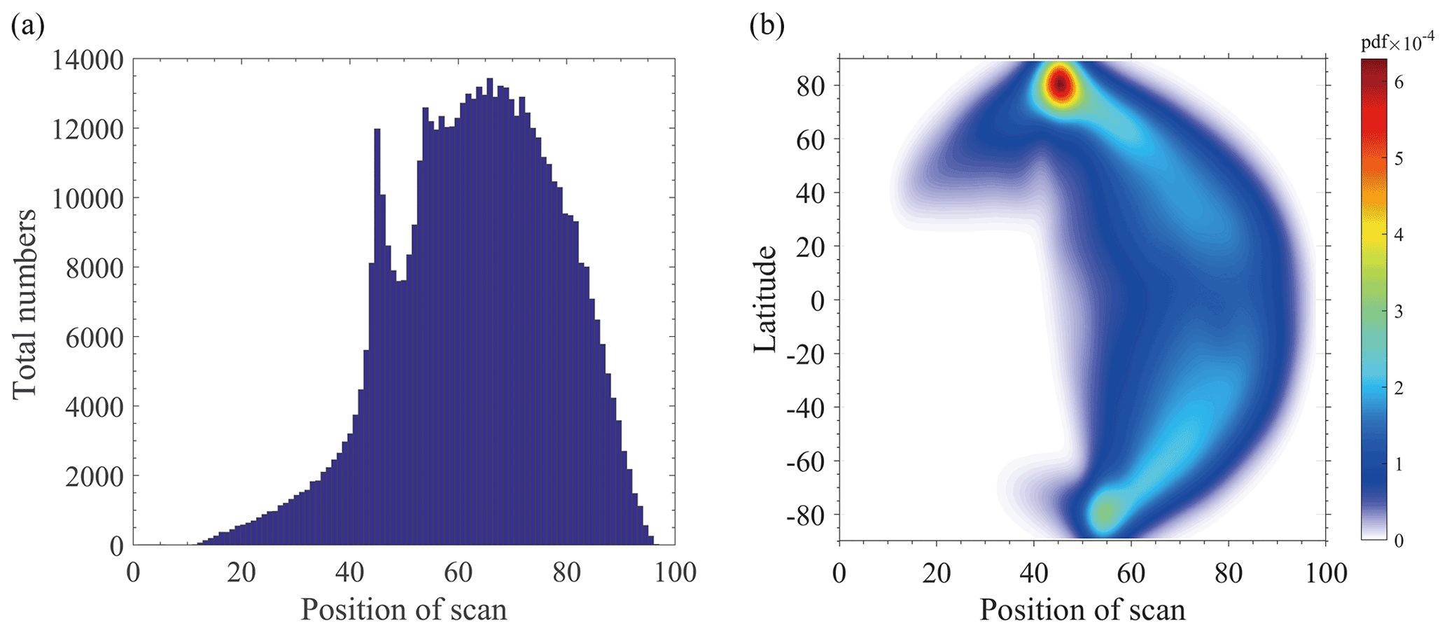
Figure 2Statistical information of the scan angle (a) and latitude (b) of MWHS observations in the collocation dataset.
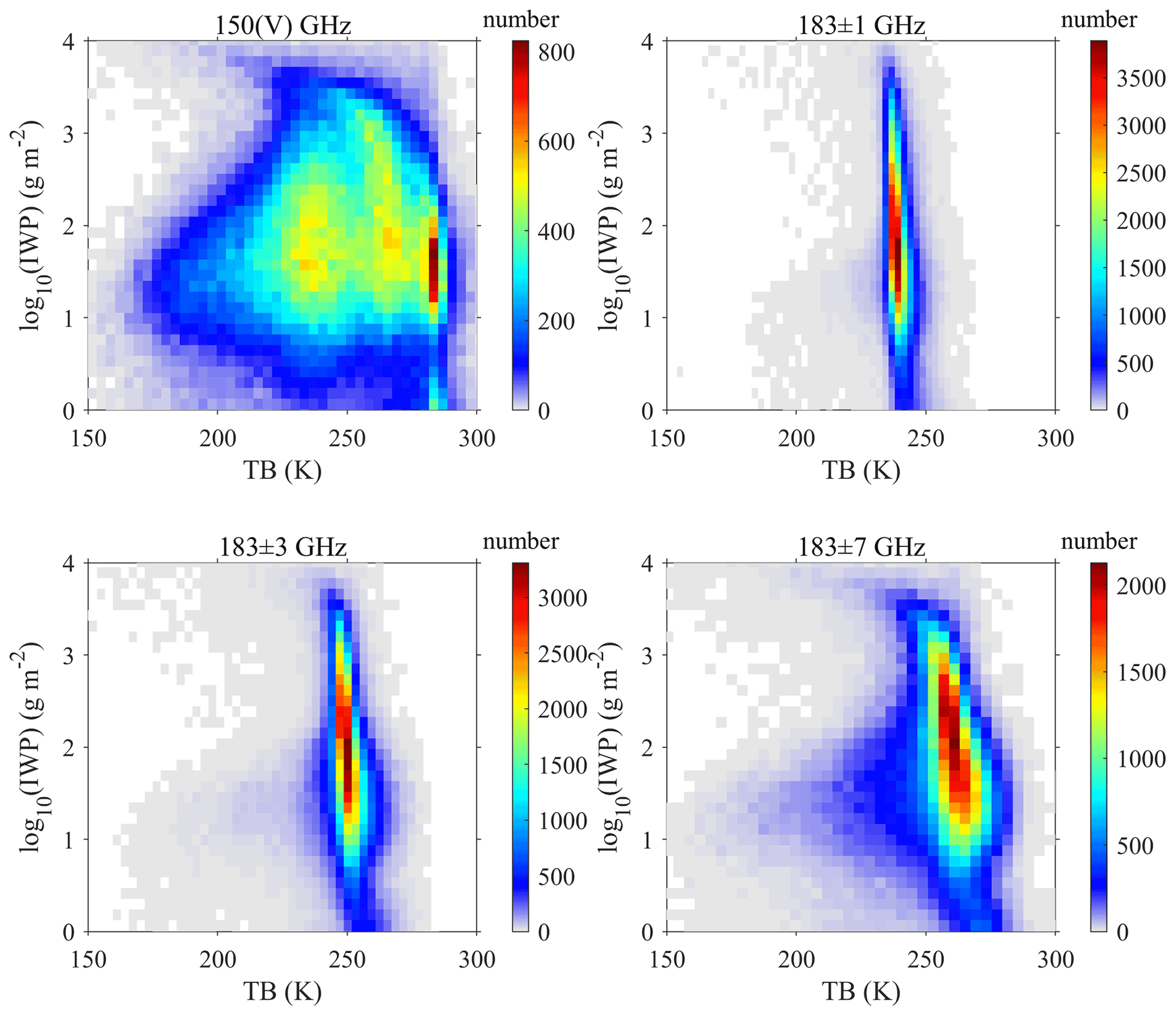
The statistical information of TB and IWP for different channels (CH.2–CH.5) in the collocation dataset is given in Fig. 4. The TBs for CH.3 and CH.4 were mainly concentrated at approximately 250 K, indicating a small sensitivity to ice clouds. For CH.2 and CH.5, the TBs had a larger range of variation, which is due to the larger contribution of near-surface information to the window channels. However, it can be seen that, in the presence of ice clouds (IWP >100 g m−2), the surface information is blocked by clouds, making the TB range significantly smaller as the IWP becomes larger. The statistical relationship between the 150 GHz TB and IWP at different scan angles is given in Fig. 5. It can be found that there is a significant decrease in the measured TB with increasing IWP for large scan angles. As the scan angle decreases, especially in the case of nadir observations, many low TBs are appearing in clear-sky scenes because nadir observations have a very large number of collocation scenes in the polar regions (see Fig. 2b) where the surface lowers the measured TB. In contrast, collocation scenes with large scan angles are mainly located in the tropics, which makes the TB–IWP relationship very significant.

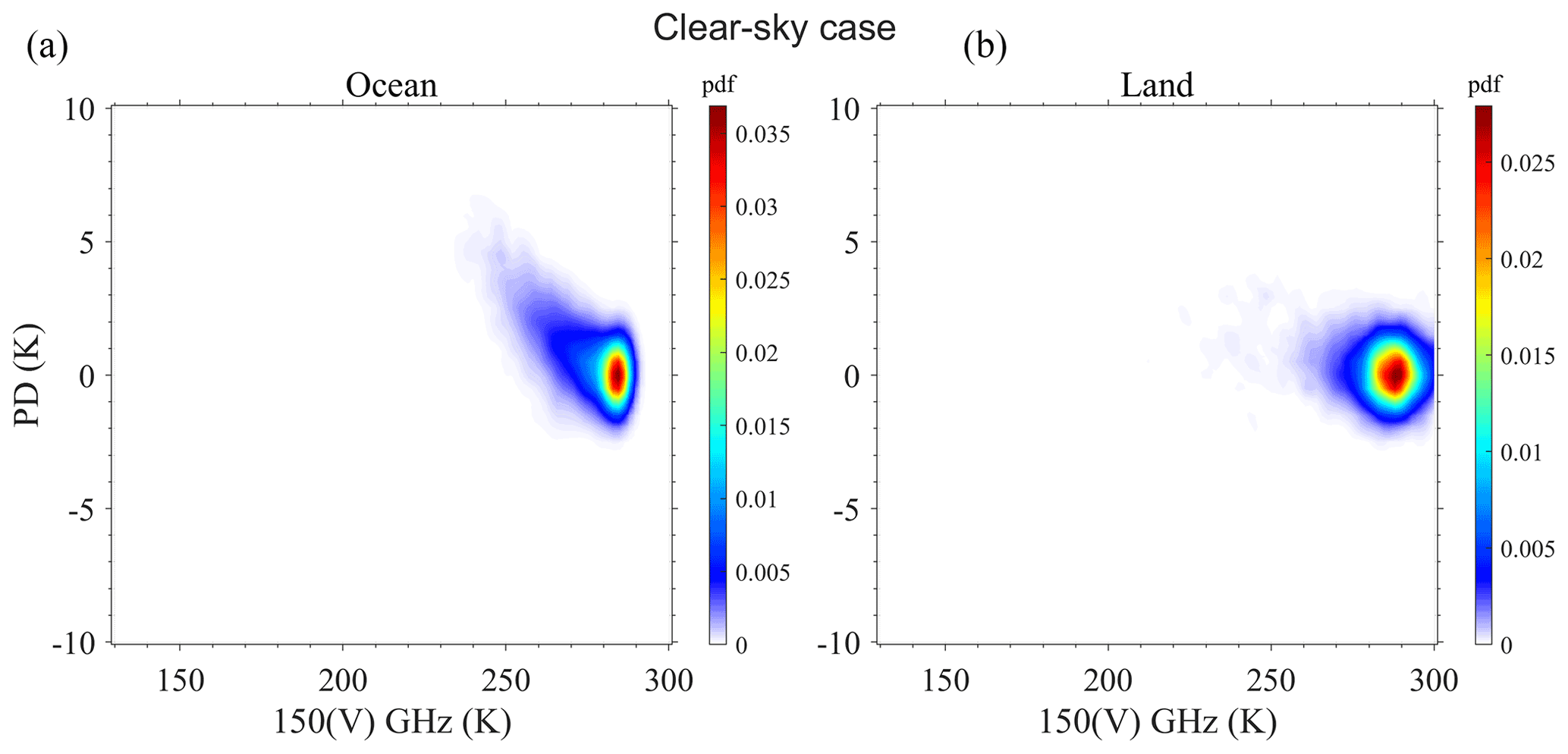
The density plots of the PD and TB at 150 GHz (clear-sky and cloudy scenes) and the corresponding IWP from 2C-ICE over the ocean and land are depicted in Figs. 6 and 7. Scan angles from ±41.28 to ±53.35∘ were selected to compare the results with observations from conical scanners. In the cloudy case, the TBs are distributed between 150 and 290 K, with the largest PD occurring at 230 K (corresponding to IWP >1000 g m−2). This is similar to the result of Gong and Wu (2017) and Gong et al. (2020). However, due to the quasi-polarization mode and the much larger footprint, the PD of MWHS is much lower than that of conical scanners (e.g. GMI). The lowest TB generally appears in the centre of deep convection clouds, and the PD is small due to the randomly oriented ice particles; the largest PD due to the horizontally oriented particles generally appears in the warmer clouds. Figure 6 shows that, the lower the TB, the larger the IWP, while the TB is also influenced by the local atmospheric temperature. Comparing Figs. 6 and 7, the TB of the clear sky is generally above 240 K. The PD from the ocean surface is relatively large, while the PD from land is small.

Figure 6The PD–TB150 V density plots for the collocations in the cloudy scenes over the ocean (a) and land (b). Panels (c) and (d) show the corresponding IWPs from 2C-ICE.
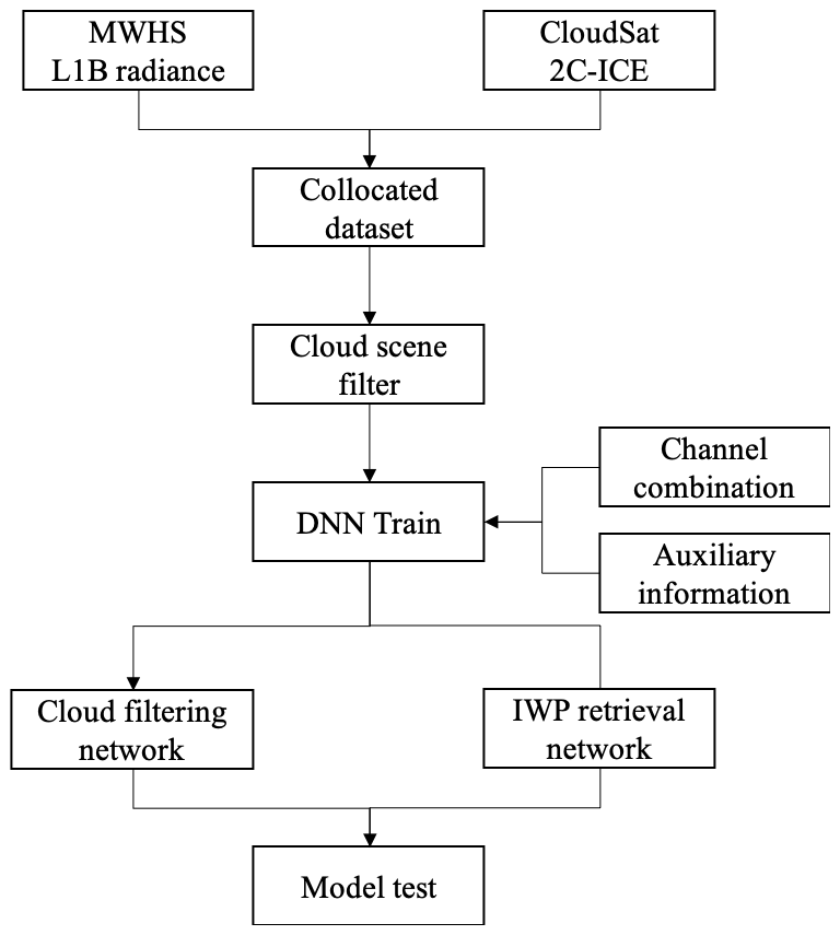
The collocations were used as a retrieval dataset to train the networks, and the processing flow is shown in Fig. 8. The DNN is a feed-forward neural network that contains an input layer, several hidden layers, and an output layer. The DNN is a fully connected network, and neurons in each layer connect with all neurons in the next layer. The hidden layers are used to perform the nonlinear calculation to achieve a nonlinear mapping from the input to the output data. The outstanding nonlinear mapping capability makes DNNs popular for geophysical retrieval.
In this study, a DNN with six layers was selected. The first layer was the input layer, and each input quantity used a neuron to connect with the next layer. The second to fifth layers were the hidden layers in which 256 neurons were used for each layer, and the tanh and the rectified linear unit (ReLU) are selected as the activation functions for the cloud filtering network and the IWP retrieval network, respectively. Since networks are prone to overfitting in the training, the early stopping and dropout method is used to improve the training. To remove the effect of the order of data, random assignation and normalization are performed in front of the hidden layers. The final layer was the output layer, which used the IWP of 2C-ICE (transfer to log space) as a reference. The activation function of the last layer is selected according to the target of the network. For the determination of cloudy and clear-sky scenes, the sigmoid function was used for binary classification. For the IWP retrieval, the results were output directly. Due to the imbalanced dataset of the clear-sky and cloudy scenes, the focal loss function which can solve the problem of a serious imbalance of positive and negative sample ratios in one-stage object detection was used instead of the cross-entropy loss function (Lin et al., 2017). In the iterative training of the networks, the models with the best results in the validation data will be retained. The hyperparameters were chosen by comparing the performance of DNNs with different hidden layers, numbers of hidden neurons, and regularization parameters. Each network mentioned in the next section uses the same hyperparameters of the model to ensure that the performance of the network is only affected by the input parameters.
The sensitivity of ice clouds was discussed by Holl et al. (2010) and Eliasson et al. (2013), and their studies showed no significant radiance signals at IWPs <100 g m−2 for MHS measurements. Therefore, it was used as the threshold for the cloud filtering network.
From those collocations, we randomly assign 75 % to be used for training and 25 % to be used for validation. The training data are used as a sample of the data for model fitting. The validation data can be used to tune the hyperparameters of the network and for preliminary evaluation of the model. Collocations during January 2015 are used for testing. These data were not used to train the networks and adjust the hyperparameters but serve as independent data to test the performance of the final obtained networks.
The performance metrics employed for the retrieval are defined in the following. The commonly used binary classification metrics are chosen for the cloud filtering network. A confusion matrix M is defined as follows:
TP and TN are the number of true positives (both MWHS and CloudSat find ice clouds) and negatives (both MWHS and CloudSat find no ice clouds), respectively. FP and FN are the number of false positives (MWHS finds ice clouds but CloudSat does not) and negatives (CloudSat finds ice clouds but MWHS does not), respectively.
From the confusion matrix above, the accuracy (AC), false alarm ratio (FAR), probability of detection (POD), F1 score and critical success index (CSI) can be derived as follows:
The performance evaluation for the IWP retrieval network is based on the root mean square error (RMSE), mean absolute percentage error (MAPE), bias (BIAS), and Pearson correlation coefficient (CC) and defined as follows:
To retrieve the IWP from the MWHS measurements, two networks were trained for different capabilities. The first one allowed classifying a scene according to whether it is clear sky or cloudy. The second was to retrieve the IWP. The two networks are used separately, and the IWP of the scene considered clear sky was set to 0. Due to the randomness of the neural network in the assigned training and validation data, 20 models were trained for each combination to ensure the stability of the model results.
4.1 Cloud filtering network
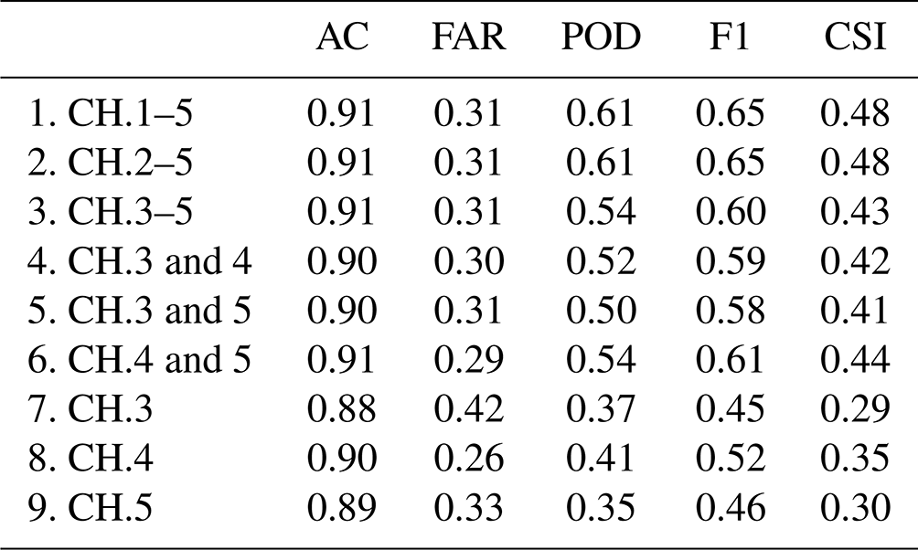
The network structure, training dataset, and cloud IWP threshold are discussed above. The sigmoid activation function can vary the output of the network from 0 to 1, which represents the probability of cloud occurrence. Therefore, a threshold value of cloud probability must be assigned to determine the cloudy scene. After testing, a threshold value of 0.4 was the most appropriate for this cloud filtering. To enhance the filtering capacity, scan angle, mask, latitude, and longitude were all used as auxiliary information. The cloud filtering performance for different channel combinations is listed in Table 2. The results showed that all three 183 GHz channels have cloud identification capability, and the addition of one 150 GHz channel enhances the POD of the network, while the two 150 GHz channels do not yield additional information. However, the detection of ice clouds using MWHS channels was still limited. The FAR and POD of the best network are 0.31 and 0.61, respectively.
4.2 IWP retrieval network
For the global IWP retrieval, clear-sky scenes were excluded from the training data. Different combinations of the network input are compared to find the best retrieval strategy. The auxiliary information cases and their retrieval errors are listed in Table 3. In these cases, all five channels were used. Additional information, including latitude, scan angle, and ocean/land mask and their combinations, was added to train the networks.
Table 3Errors in IWP retrieval using different auxiliaries. Note: NO is for no auxiliaries, Lat is adding latitude as auxiliary information, Ang is adding the scan angle, and Mask is adding the land/sea mask.
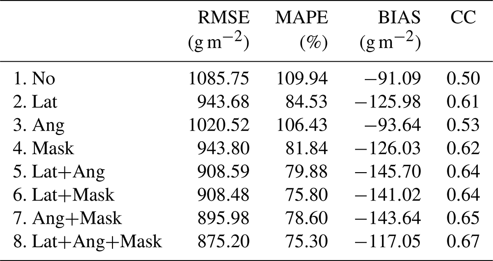
Concerning the errors shown in Table 3, a significant improvement in retrieval performance is achieved by adding latitude or ocean/land mask information, while the contribution of just adding the scan angle to the retrieval is not significant. In MWHS measurements, the signal from ice clouds is a reduction in TB by the scattering effect. In the absence of latitude information and ocean/land mask, it is difficult to distinguish whether the decrease in TB is due to ice particles or the low radiance from the surface. According to cases 1, 2, and 4 in Table 3, CC is improved from 0.50 to approximately 0.62, and the RMSE and MAPE are also improved significantly. However, MAPE and BIAS are in conflict, and reducing MAPE will increase BIAS. Therefore, CC is an important metric for evaluating the model. The combination of auxiliaries can further improve the retrieval results, although the effect of using the scan angle alone is not obvious. Cases 5 and 6 in Table 3 indicate that the scan angle combined with latitude and ocean/land mask can also further improve the retrieval capability. The retrieval MAPE of each IWP bin is shown in Fig. 9a. The MAPE in different IWP bins gives a more detailed comparison. Compared to no auxiliary model, adding auxiliaries can significantly reduce retrieval errors, especially at IWP <200 g m−2 and IWP >1000 g m−2.
The performance of the different channel combinations (all the auxiliary information is added) is presented in Table 4. Since the 183 GHz channels (CH.3–5) of MHS have proven to have good sensitivity to CloudSat IWP, the influence of the 150 GHz channel and its PD were mainly focused on here. The results of cases 2 and 3 in Table 4 show that adding the 150 GHz window channel (CH.2) gives an improvement to all the metrics. Considering the contribution of PD in the retrieval, the results show that the addition of PD alone (case 4) contributes to the retrieval of IWP, while the combination including both H and V polarization channels has the best performance (case 1). Figure 9b illustrates the MAPE of different channels. Comparing case 3 with case 4 in Table 4, the addition of PD gives an obvious improvement in the retrieval results at IWP >2000 g m−2. In general, all channels of MWHS contribute to ice cloud retrieval.
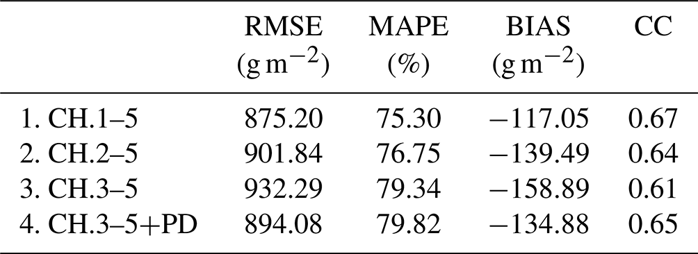
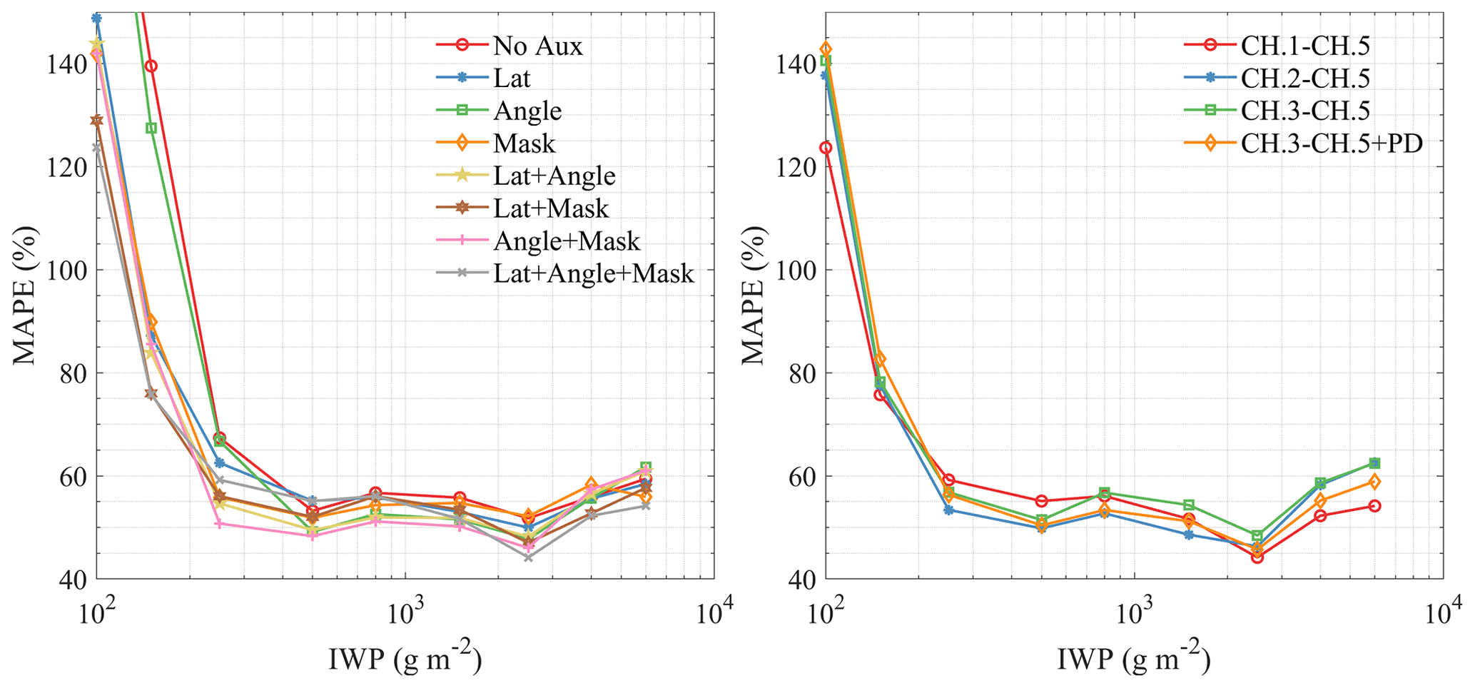
Figure 9Comparison between the performance of the IWP retrieval networks using different auxiliary and channel combinations of input.
The final retrieval models (case 1 in Table 2 and case 8 in Table 3) were selected according to the metrics. Combining the cloud filtering network and the IWP retrieval network with the test data, the final results are shown in Table 5. The performance over the ocean and land is also listed. After adding the cloud filtering network, the accuracy of the IWP retrieval decreased significantly for MAPE and BIAS and slightly for CC and RMSE. The results are better over the ocean than over land, especially the correlation. Figure 10 shows the scatterplot between MWHS IWP and 2C-ICE IWP in January 2015. The result shows relative agreement, but the MWHS IWP has significant dispersion at low IWPs, which may be due to the lack of sensitivity of the MWHS to thin ice clouds. Although the MWHS channels are sensitive to the IWP when it is around 100 g m−2, the cloud filtering network shows large FAR, which will lead to unsatisfactory results at the IWP threshold. The final model underestimates the true value overall but overestimates it when the IWP <300 g m−2.
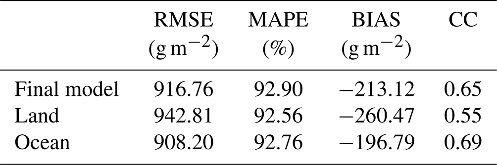
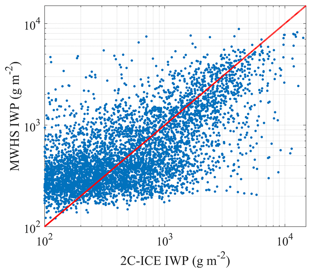
Figure 10Comparison between 2C-ICE and MWHS IWP. The red line represents the diagonal 1:1 line. Clear-sky scenes are not shown.
4.3 Network application
4.3.1 Tropical cyclone IWP retrieval
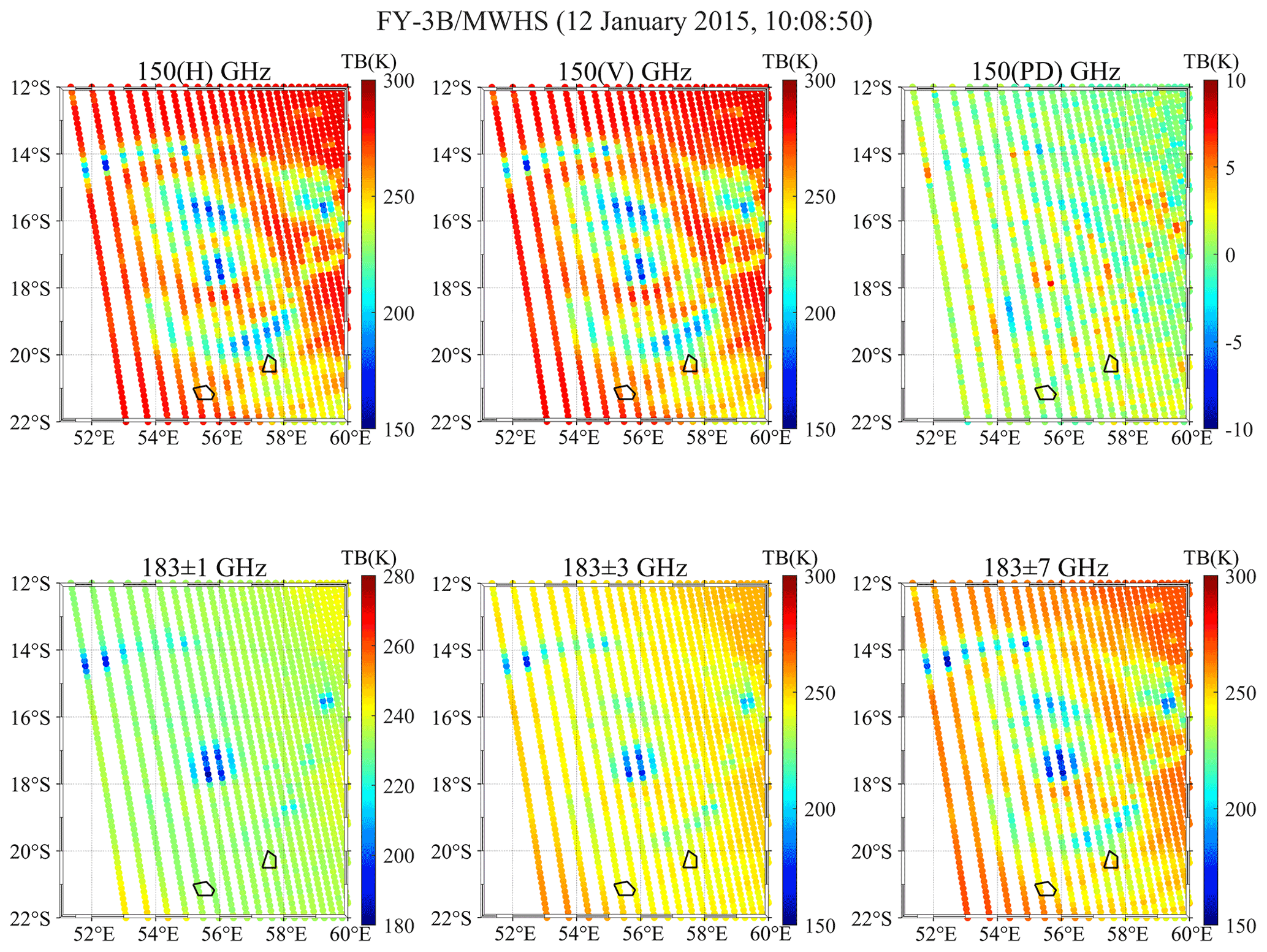
Tropical Cyclone Bansi, observed by MWHS and CloudSat simultaneously (the time difference is approximately 3 min) on 12 January 2015, was selected for the validation of the final networks. The MWHS-observed TBs of the cyclone are shown in Fig. 11. Quite low TB (as low as 150 K) can be found at 150 and 183±7 GHz channels in the regions of the eyewall (the eye is not seen) and spiral rain bands which were mainly caused by the scattering of ice particles in the clouds. The 183±1 and 183±3 GHz channels were strongly influenced by water vapour, and the shape of the cyclone was hardly observable, but clear low TBs can still be seen in the eyewall and rainband. The distribution characteristics of PDs at 150 GHz (TBV−TBH) are similar to the structure of the tropical cyclone, but significant PDs occur mainly in the warm ice clouds at approximately 200–250 K. The PD reaches its maximum in the anvil precipitation regions (approximately 5 K; consistent with the result in Fig. 4) and decreases in the remote clear-sky or cirrus regions.
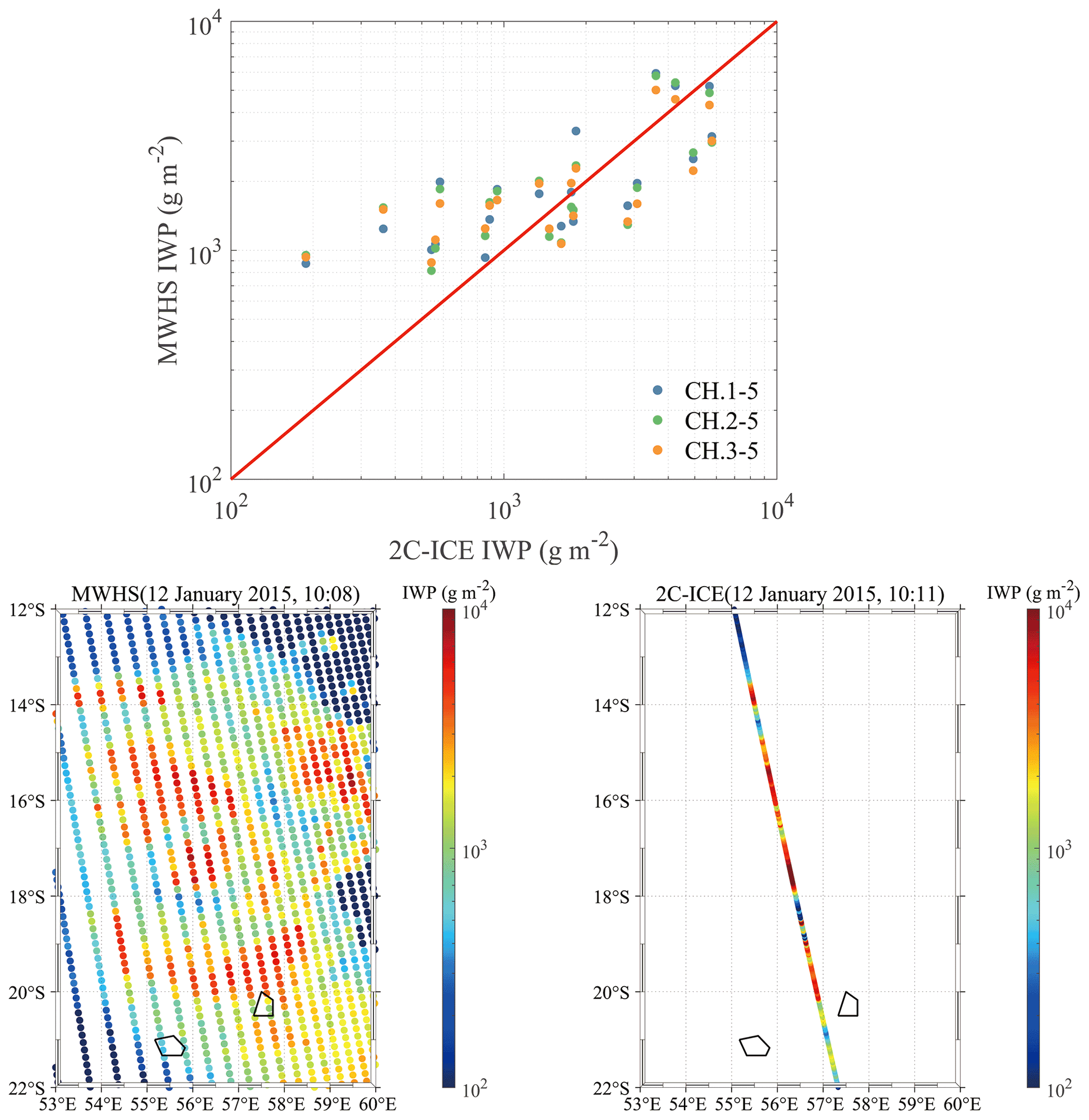
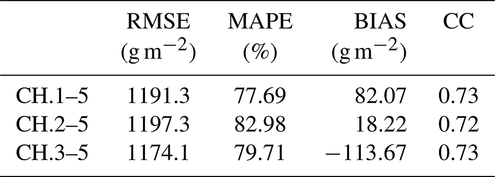
Applying the two neural networks trained above to the tropical cyclone, the retrieval IWPs are shown in Fig. 12 in comparison with 2C-ICE, and the retrieval errors are listed in Table 6. Due to the narrow field of view of CloudSat, a total of 21 pixels of MWHS were collocated in the tropical cyclone region. The results show that MWHS IWP has a high correlation with 2C-ICE, and the MAPE and BIAS in the tropical cyclone cases are better than those in Table 5. Although the RMSE is larger, it is reasonable in tropical cyclones. For tropical cyclone retrieval, the addition of the 150 GHz channel does not have a significant impact on the accuracy. The RMSE and CC of the three retrievals are similar. Although there are differences between MAPE and BIAS, the differences are not significant.
4.3.2 Global mean IWP comparison
Figure 13 gives the TB of each channel against that of all the other channels for the MWHS dataset in 2015 (blue) and the collocation dataset (red). Due to a huge amount of MWHS data, 106 measurements were randomly selected for each month, i.e. a total of 1.2×10⁷ samples. Overall, the collocation dataset covers a most range of the measurements, which means that the collocations are well representative of the MWHS measurement scenes.
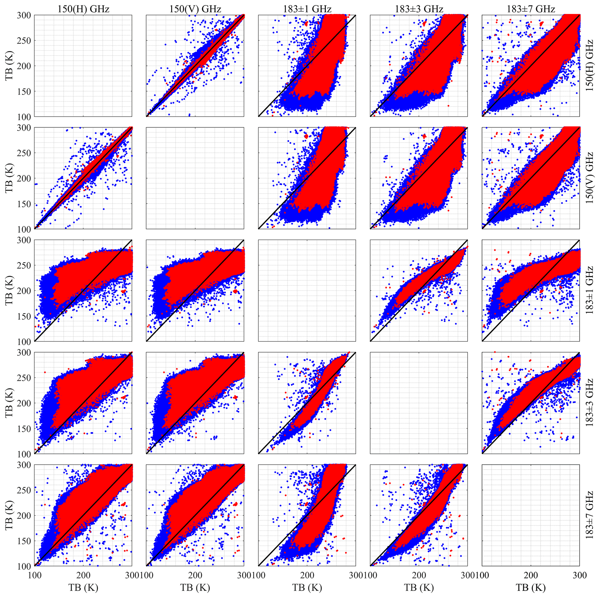
Figure 13Measurement comparison from different channels of MWHS dataset in 2015 (blue) and the collocation dataset discussed above (red).
Figure 14 shows the global mean IWP for 2015 from the Aqua/MODIS L3 product (MYD08_M3, C61; Platnick et al., 2015), CloudSat 2C-ICE, FY-3B/MWHS retrieval, and ERA5 reanalysis dataset. The ERA5 IWP data shown here were combined from the total column snow water (CSW) and cloud ice water (CIW) data since they differentiate between precipitating and nonprecipitating ice. The overall distribution of the annual mean IWP for the four datasets is similar. The MODIS product has a significantly higher IWP than the other three products, while ERA5 has a lower IWP overall. The IWP from 2C-ICE is the same as MODIS near the Equator and between ERA5 and MODIS elsewhere. Since 2C-ICE was used to train the networks, MWHS IWP is certainly approaching the 2C-ICE and similar to the IWP maps in Duncan and Eriksson (2018). There is no significant difference between the results of the three MWHS channel combinations on the map, but the IWP result using only the 183 GHz channels is lower at middle latitudes than the IWP results with the addition of the 150 GHz channels. The zonal means of IWP for 2015 are given in Fig. 15. The overall shape of the IWP zonal averages is fairly consistent across datasets. However, there are large differences in the overall magnitude of the IWP. These differences are particularly pronounced at mid-latitudes, especially between the MODIS product and the other three products. The IWP from MWHS is generally close to 2C-ICE, and the result without the 150 GHz channel is lower than 2C-ICE between 30 and 60∘ S in the Northern Hemisphere and 20–60∘ N in the Southern Hemisphere. There is an improvement after adding the 150 GHz channel (little difference between using 1 or 2 150 GHz channels), and the IWP in the Northern Hemisphere is the same as the 2C-ICE, while it is still lower in the Southern Hemisphere.
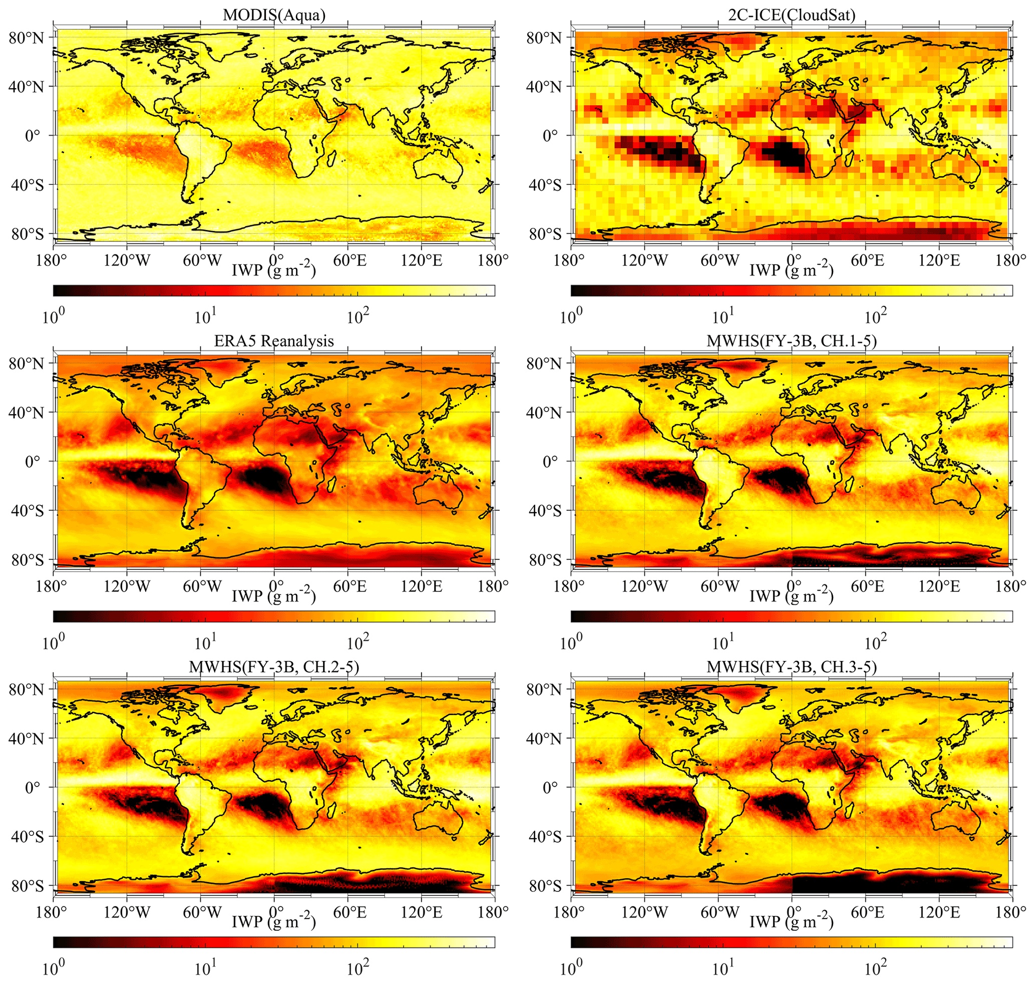
Figure 14Global mean IWP maps for 2015 from MODIS, 2C-ICE, ERA5, and different channel combinations from MWHS. The 2C-ICE is gridded on a 5∘ grid, while the other products are gridded on a 1∘ grid.
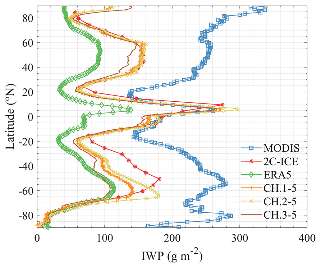
Figure 15Zonal means of IWP for 2015 from MODIS, 2C-ICE, ERA5, and different channel combinations from MWHS. The 2C-ICE is gridded on a 5∘ grid, while the other products are gridded on a 1∘ grid.
4.4 Discussion
Ice cloud misidentification is an important and unavoidable problem in this study. One reason is that the microwave channels detect ice clouds through the large decrease in TB. However, the low temperature in high-altitude regions or other temperature anomaly phenomena can also lead to low TB. In the final results above, although geographic information is added to the training data, there are still many misclassification cases, such as on the Tibetan Plateau in winter. Therefore, knowing the surface temperature or the near-surface air temperature will help ice cloud detection. Holl et al. (2014) show that infrared channels show good performance. The other reason is due to the mismatch between the CloudSat and the MWHS footprints spatially and temporarily. Since the CloudSat pixels cover less than 15 % of the MWHS pixels, the 2C-ICE scenes cannot fully represent the MWHS observations, especially in the case of thin clouds.
For the IWP retrieval, the 150 GHz window channel has a significant ice cloud response which, in combination with 183 GHz channels, provides a better retrieval of IWP. The PD at 150 GHz, although contaminated by polarization from the ocean surface, also contributes positively to the retrieval especially when the IWP is larger than 1000 g m−2. In addition, the PD of quasi-polarization channels from MWHS is related to the scan angle and does not fully represent the polarization information of the ice particles, especially near the 45∘ scan angle. From the perspective of polarization measurements only, a cross-track scanner does not provide as much polarization information as a conical scanner.
In terms of the retrieval using the neural network, the results of this paper are basically consistent with Holl et al. (2014). The error between the retrieval results and 2C-ICE is approximately 100 %. The latitude and ocean/land mask are important auxiliary information for DNN retrieval. Holl et al. (2014) used angle information that contains geometric observations of the local zenith and azimuth and showed a significant improvement. However, the results in Table 3 show that the scan angle is of limited help for retrieval, which may be due to the fact that the scan angle is not fully representative of the geometry of the observed radiance, and it works better when used in conjunction with the latitude and land/sea mask.
However, there are some limitations to using neural networks for IWP retrieval. Collocation is the first limitation, since there are some uncertainties in the field of view of MWHS and CloudSat due to the large resolution difference. These uncertainties are represented in the training data and can be better predicted using, for example, quantile regression neural networks (Pfreundschuh et al., 2018). The most important issue is the real sample (2C-ICE) used in training, which has uncertainties that are difficult to quantify. Therefore, it is also impossible to make accurate error estimates of the model results. In the absence of access to a large number of real samples, the use of neural networks can only converge to a certain product with the highest accuracy (such as 2C-ICE). An alternative approach is to use simulation results (typical profiles) of radiative transfer models, where the generalization ability of the network will strongly depend on the model itself and the input field. In addition, the microwave band below 200 GHz is sensitive only to large ice particles and thick clouds and is relatively less effective for cloud detection.
In this paper, an analysis of global IWP retrieval from FY-3B/MWHS radiance measurements based on neural networks is presented. The MWHS aboard the FY-3B satellite has two quasi-polarization channels at 150 GHz, which can provide more information about ice clouds. For IWP retrieval, CloudSat/2C-ICE was chosen as the reference dataset for neural networks because it is publicly available and meets the requirements in terms of data numbers and measurement accuracy. Two types of networks (cloud filtering and IWP retrieval) are trained using the collocation dataset of MWHS and 2C-ICE. A cloud filtering network was trained to classify cloudy and clear-sky scenes. For the IWP threshold of 100 g m−2, 183 GHz channels of MWHS show sensitivity to ice clouds, and 150 GHz channels improve the performance. The FAR and POD of the final network are 0.31 and 0.61, respectively. IWP retrieval networks with different combinations of channels and auxiliary information as input were compared to find the best retrieval strategy. The retrieval results show that adding the 150 GHz channel gives an obvious improvement in IWP retrieval and that the PD also has a positive impact. Comparing the final configuration MWHS retrieval IWP with 2C-ICE, the CC =0.65, RMSE =916.76 g m−2, MAPE =92.90 %, and BIAS g m−2.
Applying the networks to Tropical Cyclone Bansi, the results show a relatively high correlation (0.73) between MWHS IWP and 2C-ICE. In this case, the effect of the 150 GHz channel is not significant compared to using only 183 GHz channels. The 2015 annual mean IWP from MWHS shows a similar overall shape to that of MODIS, 2C-ICE, and ERA5 and is very close to 2C-ICE in magnitude, making the retrieved IWP more credible. Compared with the result using only 183 GHz channels, adding 150 GHz channels significantly improves the retrieval accuracy in the mid-latitude region.
Neural networks are widely used to statistically characterize the mapping between radiometric measurements and related geophysical variables. The advantages of neural networks are their simplicity and ease of use, their ability to effectively learn the complex nonlinear mapping relationships in samples, and their better robustness to noisy data. By using collocated measurements, there is no need to establish a complicated radiative transfer model with many possible sources of error. Although the retrieval accuracy can never be as good as 2C-ICE, the spatial and temporal coverage will be much larger which is important for a long time series of climate research.
FY-3B MWHS data are available at: http://satellite.nsmc.org.cn/PortalSite/Data/Satellite.aspx?currentculture=en-US (last access: 26 October 2022; National Satellite Meteorological Center, 2015.). CloudSat 2C-ICE product can be downloaded from https://www.cloudsat.cira.colostate.edu/data-products (last access: 20 October 2022; CIRA, 2019). Aqua/MODIS L3 product can be downloaded from https://ladsweb.modaps.eosdis.nasa.gov/search/order/1/MYD08_M3--61 (last access: 22 March 2022; LAADS DAAC, 2022). ERA5 reanalysis data can be downloaded from https://doi.org/10.24381/cds.6860a573 (Hersbach et al., 2019). The code and test data for this paper are accessible from public repositories (https://doi.org/10.5281/zenodo.6620750; Wang, 2022).
ZW and WW designed the study. WW performed the implementation and wrote the paper. QH and LZ provided the training data and established the network model. ZW revised the article.
The contact author has declared that none of the authors has any competing interests.
Publisher's note: Copernicus Publications remains neutral with regard to jurisdictional claims in published maps and institutional affiliations.
The authors would like to thank the National Satellite Meteorological Center, China Meteorological Administration, for providing the FY-3B MWHS data. The authors thank the CloudSat and CALIPSO science teams, for their efforts in providing the 2C-ICE product. The authors also thank the MODIS and ERA5 teams, for providing the Aqua/MODIS L3 product and ERA5 reanalysis data. We would also like to thank the reviewers and the editors, for their valuable and helpful suggestions.
This work has been supported by the National Natural Science Foundation of China (grant nos. 42105130 and 41901297) and the Science and Technology Key Project of Henan Province (grant no. 202102310017).
This paper was edited by S. Joseph Munchak and reviewed by two anonymous referees.
Austin, R. T., Heymsfield, A. J., and Stephens, G. L.: Retrieval of ice cloud microphysical parameters using the CloudSat millimeter-wave radar and temperature, J. Geophys. Res., 114, D00A23, https://doi.org/10.1029/2008JD010049, 2009.
Bennartz, R. and Bauer, P.: Sensitivity of microwave radiances at 85–183 GHz to precipitating ice particles, Radio Sci., 38, 8075, https://doi.org/10.1029/2002RS002626, 2003.
Boukabara, S.-A., Garrett, K., Chen, W., Iturbide-Sanchez, F., Grassotti, C., Kongoli, C., Chen, R., Liu, Q., Yan, B., Weng, F., Ferraro, R., Kleespies, T. J., and Meng, H.: MiRS: An All-Weather 1DVAR Satellite Data Assimilation and Retrieval System, IEEE. T. Geosci. Remote., 49, 3249–3272, https://doi.org/10.1109/tgrs.2011.2158438, 2011.
Brath, M., Fox, S., Eriksson, P., Harlow, R. C., Burgdorf, M., and Buehler, S. A.: Retrieval of an ice water path over the ocean from ISMAR and MARSS millimeter and submillimeter brightness temperatures, Atmos. Meas. Tech., 11, 611–632, https://doi.org/10.5194/amt-11-611-2018, 2018.
Brath, M., Ekelund, R., Eriksson, P., Lemke, O., and Buehler, S. A.: Microwave and submillimeter wave scattering of oriented ice particles, Atmos. Meas. Tech., 13, 2309–2333, https://doi.org/10.5194/amt-13-2309-2020, 2020.
Buehler, S. A., Jimenez, C., Evans, K. F., Eriksson, P., Rydberg, B., Heymsfield, A. J., Stubenrauch, C. J., Lohmann, U., Emde, C., John, V. O., Sreerekha, T. R., and Davis, C. P.: A concept for a satellite mission to measure cloud ice water path, ice particle size, and cloud altitude, Q. J. Roy. Meteor. Soc., 133, 109–128, https://doi.org/10.1002/qj.143, 2007.
Buehler, S. A., Defer, E., Evans, F., Eliasson, S., Mendrok, J., Eriksson, P., Lee, C., Jiménez, C., Prigent, C., Crewell, S., Kasai, Y., Bennartz, R., and Gasiewski, A. J.: Observing ice clouds in the submillimeter spectral range: the CloudIce mission proposal for ESA's Earth Explorer 8, Atmos. Meas. Tech., 5, 1529–1549, https://doi.org/10.5194/amt-5-1529-2012, 2012.
CIRA (Cooperative Institute for Research in the Atmosphere): Cloudsat and CALIPSO Ice Cloud Property Product, CloudSat Data Processing Center [data set], https://www.cloudsat.cira.colostate.edu/data-products/2c-ice (last access: 20 October 2022), 2019.
Coy, J. J., Bell, A., Yang, P., and Wu, D. L.: Sensitivity Analyses for the Retrievals of Ice Cloud Properties From Radiometric and Polarimetric Measurements in Sub-mm/mm and Infrared Bands, J. Geophys. Res.-Atmos., 125, e2019JD031422, https://doi.org/10.1029/2019JD031422, 2020.
Defer, E., Galligani, V. S., Prigent, C., and Jimenez, C.: First observations of polarized scattering over ice clouds at close-to-millimeter wavelengths (157 GHz) with MADRAS on board the Megha-Tropiques mission, J. Geophys. Res.-Atmos., 119, 12301–12316, https://doi.org/10.1002/2014jd022353, 2014.
Delanoë, J. and Hogan, R. J.: Combined CloudSat-CALIPSO-MODIS retrievals of the properties of ice clouds, J. Geophys. Res., 115, D00H29, https://doi.org/10.1029/2009JD012346, 2010.
Deng, M., Mace, G. G., Wang, Z., and Okamoto, H.: Tropical Composition, Cloud and Climate Coupling Experiment validation for cirrus cloud profiling retrieval using CloudSat radar and CALIPSO lidar, J. Geophys. Res., 115, D00J15, https://doi.org/10.1029/2009JD013104, 2010.
Deng, M., Mace, G. G., Wang, Z., and Lawson, R. P.: Evaluation of Several A-Train Ice Cloud Retrieval Products with In Situ Measurements Collected during the SPARTICUS Campaign, J. Appl. Meteorol. Clim., 52, 1014–1030, https://doi.org/10.1175/JAMC-D-12-054.1, 2013.
Duncan, D. I. and Eriksson, P.: An update on global atmospheric ice estimates from satellite observations and reanalyses, Atmos. Chem. Phys., 18, 11205–11219, https://doi.org/10.5194/acp-18-11205-2018, 2018.
Eliasson, S., Buehler, S. A., Milz, M., Eriksson, P., and John, V. O.: Assessing observed and modelled spatial distributions of ice water path using satellite data, Atmos. Chem. Phys., 11, 375–391, https://doi.org/10.5194/acp-11-375-2011, 2011.
Eliasson, S., Holl, G., Buehler, S. A., Kuhn, T., Stengel, M., Iturbide-Sanchez, F., and Johnston, M.: Systematic and random errors between collocated satellite ice water path observations: BIAS AND RANDOM ERRORS OF OBSERVED IWP, J. Geophys. Res. Atmos., 118, 2629–2642, https://doi.org/10.1029/2012JD018381, 2013.
Eriksson, P., Ekström, M., Rydberg, B., and Murtagh, D. P.: First Odin sub-mm retrievals in the tropical upper troposphere: ice cloud properties, Atmos. Chem. Phys., 7, 471–483, https://doi.org/10.5194/acp-7-471-2007, 2007.
Eriksson, P., Ekelund, R., Mendrok, J., Brath, M., Lemke, O., and Buehler, S. A.: A general database of hydrometeor single scattering properties at microwave and sub-millimetre wavelengths, Earth Syst. Sci. Data, 10, 1301–1326, https://doi.org/10.5194/essd-10-1301-2018, 2018.
Eriksson, P., Rydberg, B., Mattioli, V., Thoss, A., Accadia, C., Klein, U., and Buehler, S. A.: Towards an operational Ice Cloud Imager (ICI) retrieval product, Atmos. Meas. Tech., 13, 53–71, https://doi.org/10.5194/amt-13-53-2020, 2020.
Field, P. R. and Heymsfield, A. J.: Importance of snow to global precipitation, Geophys. Res. Lett., 42, 9512–9520, https://doi.org/10.1002/2015GL065497, 2015.
Fox, S.: An Evaluation of Radiative Transfer Simulations of Cloudy Scenes from a Numerical Weather Prediction Model at Sub-Millimetre Frequencies Using Airborne Observations, Remote Sens., 12, 2758, https://doi.org/10.3390/rs12172758, 2020.
Gong, J. and Wu, D. L.: Microphysical properties of frozen particles inferred from Global Precipitation Measurement (GPM) Microwave Imager (GMI) polarimetric measurements, Atmos. Chem. Phys., 17, 2741–2757, https://doi.org/10.5194/acp-17-2741-2017, 2017.
Gong, J., Zeng, X., Wu, D. L., and Li, X.: Diurnal Variation of Tropical Ice Cloud Microphysics: Evidence from Global Precipitation Measurement Microwave Imager Polarimetric Measurements, Geophys. Res. Lett., 45, 1185–1193, https://doi.org/10.1002/2017GL075519, 2018.
Gong, J., Zeng, X., Wu, D. L., Munchak, S. J., Li, X., Kneifel, S., Ori, D., Liao, L., and Barahona, D.: Linkage among ice crystal microphysics, mesoscale dynamics, and cloud and precipitation structures revealed by collocated microwave radiometer and multifrequency radar observations, Atmos. Chem. Phys., 20, 12633–12653, https://doi.org/10.5194/acp-20-12633-2020, 2020.
He, J. and Zhang, S.: Research on cirrus clouds in Tibetan Plateau using MWHS onboard Chinese FY3B/C meteorological satellite, in: 2016 IEEE International Geoscience and Remote Sensing Symposium (IGARSS), Beijing, Beijing, China, 11–15 July 2016, IEEE, 581–584, https://doi.org/10.1109/IGARSS.2016.7729145, 2016.
Hersbach, H., Bell, B., Berrisford, P., Biavati, G., Horányi, A., Muñoz Sabater, J., Nicolas, J., Peubey, C., Radu, R., Rozum, I., Schepers, D., Simmons, A., Soci, C., Dee, D., and Thépaut, J.-N.: ERA5 monthly averaged data on pressure levels from 1959 to present, Copernicus Climate Change Service (C3S) Climate Data Store (CDS) [data set], https://doi.org/10.24381/cds.6860a573, 2019.
Heymsfield, A., Krämer, M., Wood, N. B., Gettelman, A., Field, P. R., and Liu, G.: Dependence of the Ice Water Content and Snowfall Rate on Temperature, Globally: Comparison of in Situ Observations, Satellite Active Remote Sensing Retrievals, and Global Climate Model Simulations, J. Appl. Meteorol. Clim., 56, 189–215, https://doi.org/10.1175/JAMC-D-16-0230.1, 2017.
Holl, G., Buehler, S. A., Rydberg, B., and Jiménez, C.: Collocating satellite-based radar and radiometer measurements – methodology and usage examples, Atmos. Meas. Tech., 3, 693–708, https://doi.org/10.5194/amt-3-693-2010, 2010.
Holl, G., Eliasson, S., Mendrok, J., and Buehler, S. A.: SPARE-ICE: Synergistic ice water path from passive operational sensors, J. Geophys. Res.-Atmos., 119, 1504–1523, https://doi.org/10.1002/2013JD020759, 2014.
King, M. D., Tsay, S.-C., Platnick, S. E., Wang, M., and Liou, K.-N.: Cloud retrieval algorithms for MODIS: Optical thickness, effective particle radius, and thermodynamic phase, MODIS Algorithm Theoretical Basis Document No. ATBD-MOD-05, NASA, Washington, D.C., https://atmosphere-imager.gsfc.nasa.gov/sites/default/files/ModAtmo/atbd_COP.pdf (last access: 29 October 2022), 1998.
LAADS DAAC: Aqua/MODIS L3 product, LAADS DAAC [data set], https://ladsweb.modaps.eosdis.nasa.gov/search/order/1/MYD08_M3--61, last access: 22 March 2022.
Lin, T.-Y., Goyal, P., Girshick, R., He, K., and Dollár, P.: Focal loss for dense object detection, in: 2017 IEEE International Conference on Computer Vision (ICCV), Venice, Italy, 22–29 October 2017, IEEE, 2999-3007, https://doi.org/10.1109/ICCV.2017.324, 2017.
Liou, K.-N.: Influence of Cirrus Clouds on Weather and Climate Processes: A Global Perspective, Mon. Weather Rev., 114, 1167–1199, https://doi.org/10.1175/1520-0493(1986)114<1167:IOCCOW>2.0.CO;2, 1986.
Liu, G. and Curry, J. A.: Remote Sensing of Ice Water Characteristics in Tropical Clouds Using Aircraft Microwave Measurements, J. Appl. Meteorol., 37, 337–355, https://doi.org/10.1175/1520-0450(1998)037<0337:RSOIWC>2.0.CO;2, 1998.
Liu, G. and Curry, J. A.: Determination of Ice Water Path and Mass Median Particle Size Using Multichannel Microwave Measurements, J. Appl. Meteorol., 39, 1318–1329, https://doi.org/10.1175/1520-0450(2000)039<1318:DOIWPA>2.0.CO;2, 2000.
Mace, G. G. and Deng, M.: Level 2 CloudSat-CALIPSO Combined Ice Cloud Property Retrieval Product Process Description and Interface Control Document, NASA CloudSat Project Rep. P1_R05, NASA, Washington, D.C., 2019.
Mace, G. G., Zhang, Q., Vaughan, M., Marchand, R., Stephens, G., Trepte, C., and Winker, D.: A description of hydrometeor layer occurrence statistics derived from the first year of merged Cloudsat and CALIPSO data, J. Geophys. Res., 114, D00A26, https://doi.org/10.1029/2007JD009755, 2009.
Millán, L., Read, W., Kasai, Y., Lambert, A., Livesey, N., Mendrok, J., Sagawa, H., Sano, T., Shiotani, M., and Wu, D. L.: SMILES ice cloud products, J. Geophys. Res.-Atmos., 118, 6468–6477, https://doi.org/10.1002/jgrd.50322, 2013.
National Satellite Meteorological Center: MWHS L1 Data, FENGYUN Satellite Data Center [data set], http://satellite.nsmc.org.cn/PortalSite/Data/Satellite.aspx?currentculture=en-US (last access: 26 October 2022), 2015.
Pfreundschuh, S., Eriksson, P., Duncan, D., Rydberg, B., Håkansson, N., and Thoss, A.: A neural network approach to estimating a posteriori distributions of Bayesian retrieval problems, Atmos. Meas. Tech., 11, 4627–4643, https://doi.org/10.5194/amt-11-4627-2018, 2018.
Pfreundschuh, S., Eriksson, P., Buehler, S. A., Brath, M., Duncan, D., Larsson, R., and Ekelund, R.: Synergistic radar and radiometer retrievals of ice hydrometeors, Atmos. Meas. Tech., 13, 4219–4245, https://doi.org/10.5194/amt-13-4219-2020, 2020.
Platnick, S., King, M., and Hubanks, P.: MODIS Atmosphere L3 Monthly Product. NASA MODIS Adaptive Processing System, Goddard Space Flight Center [data set], USA, https://doi.org/10.5067/MODIS/MYD08_M3.061, 2015.
Stephens, G. L. and Kummerow, C. D.: The Remote Sensing of Clouds and Precipitation from Space: A Review, J. Atmos. Sci., 64, 3742–3765, https://doi.org/10.1175/2006JAS2375.1, 2007.
Stephens, G. L., Vane, D. G., Tanelli, S., Im, E., Durden, S., Rokey, M., Reinke, D., Partain, P., Mace, G. G., Austin, R., L'Ecuyer, T., Haynes, J., Lebsock, M., Suzuki, K., Waliser, D., Wu, D., Kay, J., Gettelman, A., Wang, Z., and Marchand, R.: CloudSat mission: Performance and early science after the first year of operation, J. Geophys. Res., 113, D00A18, https://doi.org/10.1029/2008JD009982, 2008.
Stubenrauch, C. J., Rossow, W. B., Kinne, S., Ackerman, S., Cesana, G., Chepfer, H., Girolamo, L. D., Getzewich, B., Guignard, A., Heidinger, A., Maddux, B. C., Menzel, W. P., Minnis, P., Pearl, C., Platnick, S., Poulsen, C., Riedi, J., Sun-Mack, S., Walther, A., Winker, D., Zeng, S., and Zhao, G.: Assessment of Global Cloud Data sets from Satellites: Project and Database Initiated by the GEWEX Radiation Panel, B. Am. Meteorol. Soc., 94, 1031–1049, https://doi.org/10.1175/BAMS-D-12-00117.1, 2013.
Sun, N. and Weng, F.: Retrieval of Cloud Ice Water Path from Special Sensor Microwave Imager/Sounder (SSMIS), J. Appl. Meteorol. Clim., 51, 366–379, https://doi.org/10.1175/JAMC-D-11-021.1, 2012.
Wang, W.: Data for MWHS and 2C-ICE collocations, Zenodo [data set], https://doi.org/10.5281/zenodo.6620750, 2022.
Wang, Y., Fu, Y., Fang, X., and Zhang, Y.: Estimating ice water path in tropical cyclones with multispectral microwave data from the FY-3B satellite, IEEE T. Geosci. Remote, 52, 5548–5557, 2014.
Wang, Z., Zhang, S., Li, J., Li, Y., and Wu, Q.: Thermal/vacuum calibration of microwave humidity sounder on FY-3B satellite, Strategic Study of CAE, 15, 33–46+53, https://doi.org/10.3969/j.issn.1009-1742.2013.10.005, 2013.
Weng, F. and Grody, N. C.: Retrieval of Ice Cloud Parameters Using a Microwave Imaging Radiometer, J. Appl. Meteorol., 57, 1069–1081, https://doi.org/10.1175/1520-0469(2000)057<1069:ROICPU>2.0.CO;2, 2000.
Winker, D. M., Vaughan, M. A., Omar, A., Hu, Y., Powell, K. A., Liu, Z., Hunt, W. H., and Young, S. A.: Overview of the CALIPSO Mission and CALIOP Data Processing Algorithms, J. Atmos. Ocean. Tech., 26, 2310–2323, https://doi.org/10.1175/2009JTECHA1281.1, 2009.
Wu, D. L., Jiang, J. H., Read, W. G., Austin, R. T., Davis, C. P., Lambert, A., Stephens, G. L., Vane, D. G., and Waters, J. W.: Validation of the Aura MLS cloud ice water content measurements, J. Geophys. Res., 113, D15S10, https://doi.org/10.1029/2007jd008931, 2008.
Wu, D. L., Austin, R. T., Deng, M., Durden, S. L., Heymsfield, A. J., Jiang, J. H., Lambert, A., Li, J. L., Livesey, N. J., McFarquhar, G. M., Pittman, J. V., Stephens, G. L., Tanelli, S., Vane, D. G., and Waliser, D. E.: Comparisons of global cloud ice from MLS, CloudSat, and correlative data sets, J. Geophys. Res., 114, D00A24, https://doi.org/10.1029/2008jd009946, 2009.
Zhao, L. and Weng, F.: Retrieval of Ice Cloud Parameters Using the Advanced Microwave Sounding Unit, J. Appl. Meteorol., 41, 384–395, https://doi.org/10.1175/1520-0450(2002)041<0384:ROICPU>2.0.CO;2, 2002.
Zou, X., Chen, X., and Weng, F.: Polarization signature from the FengYun-3 Microwave Humidity Sounder, Front. Earth Sci., 8, 625–633, https://doi.org/10.1007/s11707-014-0479-y, 2014.