A comparative evaluation of snowflake particle shape estimation techniques used by the Precipitation Imaging Package (PIP), Multi-Angle Snowflake Camera (MASC), and Two-Dimensional Video Disdrometer (2DVD)

Measurements of snowflake particle shape are important for studying snow microphysics. While a number of instruments exist that are capable of measuring particle shape, this study focuses on the measurement techniques of three digital video disdrometers: the Precipitation Imaging Package (PIP), the Multi-Angle Snowflake Camera (MASC), and the Two-Dimensional Video Disdrometer (2DVD). To gain a better understanding of the relative strengths and weaknesses of these instruments and to provide a foundation upon which comparisons can be made between studies using data from different instruments, we perform a comparative analysis of the shape measurement algorithms employed by each of the three instruments by applying the algorithms to snowflake images captured by PIP during the ICE-POP 2018 field campaign.

Our analysis primarily focuses on the measurement of the aspect ratio of either the particle itself, in the case of PIP and MASC, or of the particle bounding box, in the case of PIP and 2DVD. Both PIP and MASC use shape-fitting algorithms to measure aspect ratio. While our analysis of the MASC aspect ratio suggests that the measurements are reliable, our findings indicate that both the ellipse and rectangle aspect ratios produced by PIP underperformed considerably due to the shortcomings of the PIP shape-fitting techniques. We also demonstrate that reliable measurements of aspect ratio can be retrieved from PIP by reprocessing the raw PIP images using either the MASC ellipse-fitting algorithm or a tensor-based ellipse-fitting algorithm. Because of differences in instrument design, 2DVD produces measurements of particle horizontal and vertical extent rather than length and width. Furthermore, the 2DVD measurements of particle horizontal extent can be contaminated by horizontal particle motion. Our findings indicate that, although the correction technique used to remove the horizontal motion contamination performs remarkably well with snowflakes despite being designed for use with raindrops, the 2DVD measurements of particle horizontal extent are less reliable than those measured by PIP.

1 Introduction

Digital video disdrometers have been in use since the 1990s, and there are several instruments designed around using digital cameras to observe precipitation properties. The measurements from these instruments are not only critical for understanding precipitation microphysics, but are also critical for developing algorithms to retrieve microphysical properties using radar and passive microwave sensor data. Due to the variety of instruments available, issues can arise when making comparisons between studies and algorithms that are based on data from different instruments. To this end, the present study will compare measurements of the short and long dimension of particles as well as the resulting particle aspect ratio, defined as the ratio of the particle short-dimension length to the particle long-dimension length, produced by three common ground-based digital video disdrometers: the Precipitation Imaging Package (PIP; Pettersen et al., 2020, 2021), the Multi-Angle Snowflake Camera (MASC; Garrett et al., 2012), and the Two-Dimensional Video Disdrometer (2DVD; Kruger and Krajewski, 2002; Schönhuber et al., 2007, 2008).

Empirical relationships between snowflake or ice crystal size and terminal fall speed frequently use the maximum dimension of the particle as their independent variable (e.g., Locatelli and Hobbs, 1974). The more advanced relationships also incorporate the Reynolds number, which is dependent on the particle area exposed to the flow via the Best number; in some cases this area is replaced by an area ratio that is defined as the ratio between the area exposed to the flow and the area of the circumscribing circle, which is a function of the particle maximum dimension (Heymsfield and Westbrook, 2010). In this way, the terminal fall speed relationships can depend on both the equivalent diameter, which is directly tied to particle area, and the maximum dimension of the particle. Similarly, combinations of equivalent diameter and maximum dimension have also been used to estimate particle mass (e.g., von Lerber et al., 2017).

Snowflake shape is generally characterized by the aspect ratio of the snowflakes. Korolev and Isaac (2003) found that the mean aspect ratio of in-cloud ice particles varied as a function of the particle maximum dimension for particles smaller than ∼65 µm, whereas the aspect ratio of larger particles (i.e., those typical of snow) tended to vary inversely with temperature; the mean aspect ratios observed by the study were between 0.6 and 0.8, with the snowflake-sized particles tending to have mean aspect ratios closer to 0.6. To constrain radar backscatter calculations, aspect ratio is frequently prescribed, often with a mean value of 0.6 assumed (e.g., Matrosov et al., 2005), although a number of studies have performed backscatter calculations using a range of prescribed aspect ratios (e.g., Tyynelä et al., 2011; Westbrook, 2014). The reverse of this process has also been attempted: Munchak et al. (2022) used an optimal estimation technique to retrieve a number of snow microphysical properties, including aspect ratio, from a dual-frequency dual-polarization ground-based radar, albeit with mixed results.

As will be discussed in greater detail below, both PIP and MASC produce their measurements by fitting simple two-dimensional shapes (ellipses and rectangles, specifically) to two-dimensional projections of the three-dimensional snowflakes that the instruments are observing. Because snowflakes come in a large variety of shapes, especially when taking aggregate snowflakes into consideration, any attempt to use a simple shape, such as an ellipse or rectangle, to represent these particles suffers from the inherent limitation of underrepresenting the complexity of the snowflakes. Furthermore, the use of two-dimensional shapes to represent three-dimensional snowflakes adds an additional layer of limitations revolving around the degree to which the two-dimensional projection accurately represents the dimensions and orientations of the three-dimensional particle (e.g., Jiang et al., 2017). Despite these shortcomings, the measurement of snowflake dimensions based on shape fitting has proven to be a useful tool for studying snow microphysics, and understanding the relative capabilities of these measurements is critical to their successful use in research and applications.

The goal of the present study is to evaluate the techniques used by three ground-based digital video disdrometers to determine the shape of precipitation particles in terms of aspect ratio, which, as previously mentioned, is dependent on the relative lengths of the short and long dimensions of the particle. In doing so, we will provide a point of comparison for these three sensors. The next section will briefly discuss the data sets used for this study. In Sect. 3, we will provide a detailed description of each sensor and their respective processing algorithms as they relate to the particle shape. This will be followed by a description of our analysis methods in Sect. 4. Section 5 will present the results of our study. Section 6 will compare the results of the present study to the findings of previous studies. Finally, Sect. 7 will present our conclusions alongside a brief summary of the study.

2 Data

The data sets used to perform the analyses central to this study were collected during the 2018 International Collaborative Experiment for PyeongChang Olympic and Paralympics (ICE-POP; Lee and Kim, 2019; Lim et al., 2020; Tapiador et al., 2021). ICE-POP, which took place between 1 November 2017 and 17 March 2018, was an international collaboration between a number of programs and agencies, including the NASA Global Precipitation Mission (GPM) Ground Validation program and the Korean Meteorological Administration (KMA). The field campaign was designed to study winter precipitation in complex terrain and involved a number of measurement sites featuring a mixture of in situ and remote-sensing instrumentation. Of interest to the present study is the May Hills supersite (MHS; 37.6652^∘ N, 128.6996^∘ E; 789 m) as this site has collocated PIP, MASC, and 2DVD instruments and experienced frequent snow events. This study will focus on data collected during a snow event that took place on 7–8 March 2018. This event was selected as it contains both aggregate snow particles, which provide a large variety of shapes (and, therefore, aspect ratios), and lump graupel particles, which tend to be relatively spherical with high aspect ratios. Although the general presence of these habits was primarily identified through visual inspection of the PIP data, further support of their presence can be found by examining the time series of the particle size distribution, particle fall speed, and air temperature, as depicted in Fig. 1. Periods when aggregates are present can be identified by the larger equivalent diameters and slower fall speeds, and periods with lump graupel can be identified by the smaller equivalent diameters and faster fall speeds; the lump graupel can be discerned from liquid precipitation based on the below-freezing temperatures, which extend over a deep layer according to a nearby thermodynamic sounding (not shown). Data collected during snow events on 9 and 22 January 2018 were also examined but are not included here as their inclusion did not produce any notable changes in the results.

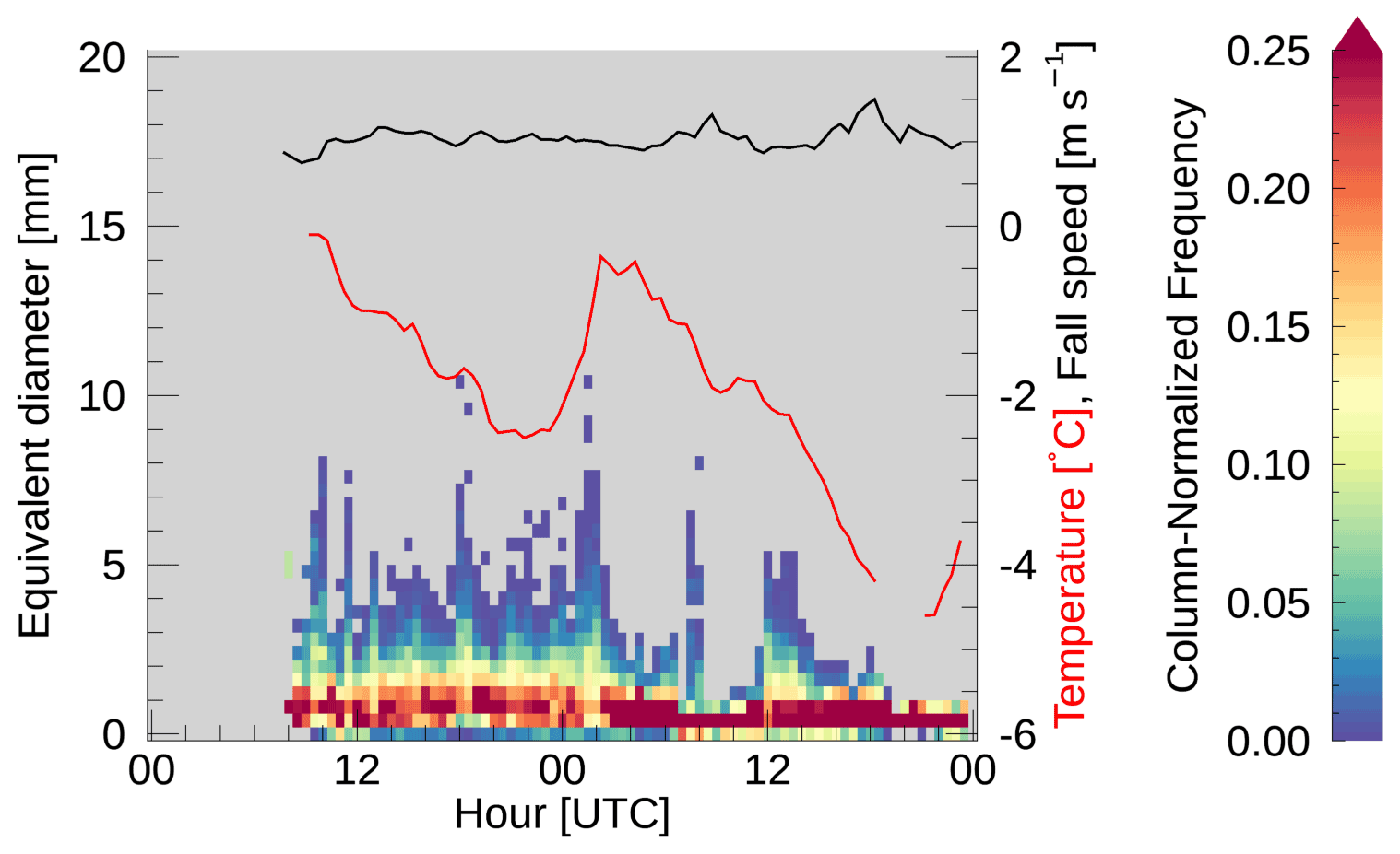
Figure 1 Time series of (shading) particle size distribution (in terms of equivalent diameter [mm]), (black) mean particle fall speed [m s⁻¹], and (red) collocated air temperature [^∘C] at the MHS site on 7–8 March 2018. Equivalent diameter and fall speed measurements come from the PIP data, and the air temperature was measured using a Vaisala WXT520. The particle size distribution time series histogram has been normalized in the y direction to emphasize the distribution within each time bin.

3 Instruments

This study will evaluate the measurement techniques of three video disdrometers: PIP, MASC, and 2DVD. The instruments and their processing algorithms, as they relate to measuring the snow particle shape, will be covered in this section.

3.1 Precipitation Imaging Package (PIP)

PIP (Pettersen et al., 2020, 2021) is a video disdrometer developed by NASA as a successor to the Snowflake Video Imager (SVI; Newman et al., 2009). PIP is composed of two parts: a high-speed video camera and a light source to backlight the precipitation particles that pass through the open sampling volume. The camera, of the charge-coupled device (CCD) variety and located 2 m from the light source, continuously records images at a rate of 380 frames per second as 640 by 480 pixel images with a pixel size of 0.1 mm by 0.1 mm using a focal plane located 1.33 m away from the camera. In order to reduce the data rate produced by the high-speed camera, the PIP images are compressed before being processed, resulting in an effective pixel size of 0.1 mm in the horizontal by 0.2 mm in the vertical. The present study uses the ICE-POP PIP data produced using version 1403 of the PIP processing code (“PIP_Rev” in the data files).

The PIP processing algorithms are written using the IMAQ Visual software package (National Instruments, 2000, 2003), a software package designed for use in performing automated quality control of manufacturing processes. Of particular interest to the present study are the methods the algorithm uses to compute the dimensions of the precipitation particle. The particle dimensions are determined by fitting an ellipse or a rectangle to the particle as viewed by PIP, which sees the two-dimensional projection of the particle, after the PIP image has been compressed to reduce data rates. The IMAQ software package performs both the ellipse and rectangle fitting by constructing an ellipse or rectangle that has an equal area and an equal perimeter to the target particle; a derivation of the equations used to make these fits is presented in Appendix A to supplement the limited information given in the IMAQ Vision manuals. According to the 2003 IMAQ Vision software manual (National Instruments, 2003), the IMAQ Vision software package computes the particle area by counting the number of pixels within a particle and the particle perimeter by subsampling the boundary points to produce a smoother representation of the perimeter; for this purpose, the boundary points are located at the corners of the pixels that make up the particle perimeter. Based on online forum discussions¹, it appears that IMAQ computes the particle perimeter from a subset of the edge pixels with the number of edge pixels skipped between each perimeter calculation pixel being a function of particle size. Unfortunately, we were unable to determine either the function relating particle size to number of skipped pixels or the corner selection method.

Once the PIP-fitted shape has been determined, the long and short axes of the fitted shapes are then used as the length and width of the particle. Specifically, the ellipse fit produces the variables “Ellip_Maj” and “Ellip_Min” for the length and width, respectively, while the rectangle fit produces the variables “Rec_BS” and “Rec_SS” for the length and width, respectively. Note, in both the ellipse and rectangle fits, the perimeter and area are defined such that any holes in the particle are not taken into account. Because of this, the PIP-determined area and perimeter of a particle with no holes will be the same as an otherwise-identical particle with a hole when determining the shape fits.

3.2 Multi-Angle Snowflake Camera (MASC)

MASC (Garrett et al., 2012) is another video disdrometer and was developed at the University of Utah; the setup described below is that used during the ICE-POP field campaign. Unlike PIP, MASC employs three cameras and only records images when triggered by a particle falling through the field of view of a pair of near-infrared sensors. The near-infrared sensors are also used to trigger a flash, which illuminates the particle from the side facing the cameras. The three cameras, also of the CCD variety and azimuthally separated from one another by 36^∘, are mounted looking into an enclosed sampling volume, open only at the top and bottom, and have a common focal point 10 cm away from each lens. Typically, the camera system is artificially restricted to only being triggered once per second in order to reduce excessive flashes. The sampling volume is defined by the intersection of the 35 mm fields of view and the 10 mm depths of field of the three cameras. While the cameras have a pixel size of 33.5 µm by 33.5 µm (Jacopo Grazioli, personal communication, 2021), the system is only triggered when particles with a maximum dimension of greater than 0.1 mm are detected by the near-infrared sensors.

Although the ICE-POP data processing for MASC uses the version of the processing algorithm written in MATLAB, a version written in Python also exists, and, for ease of implementation outside the MATLAB environment, it is this version of the ellipse fitting method that will be analyzed in this study (Shkurko et al., 2016). To simplify matching particles between the three cameras, MASC only processes images that contain a single precipitation particle, and, of these, only particles that are in focus are actually analyzed. The method used to determine whether a particle is in focus is detailed in Garrett et al. (2012). Similar to PIP, MASC also fits an ellipse to the precipitation particles to determine the particle shape properties. In the Python version of the MASC algorithm, this is accomplished using the fitEllipse function within the OpenCV package (https://docs.opencv.org/3.4/, last access: 14 November 2022), which uses the “LIN” algebraic distance ellipse-fitting algorithm described in Fitzgibbon and Fisher (1995) and returns both the major and minor axis lengths as well as the orientation angle of the fitted ellipse.

3.3 Two-Dimensional Video Disdrometer (2DVD)

2DVD (Kruger and Krajewski, 2002; Schönhuber et al., 2007) uses two orthogonally oriented horizontal line-scan cameras to take measurements of backlit precipitation particles. Since the viewing planes of the two cameras are separated by 6–7 mm, the particle fall speed can be measured via the difference in the arrival time of the particle in each viewing plane. These horizontally scanning line-scan cameras capture a series of one-dimensional images of the particle as it passes through the viewing plane. Each camera captures a one-dimensional image every 18 µs, and these one-dimensional images are then pieced together by stacking each scan on top of one another with a thickness dependent on the observed fall speed to produce a two-dimensional image of the precipitation particle for each camera. Each of the 2DVD line-scan cameras has 512 photodetectors that are calibrated to observe a 100 mm wide field of view (Kruger and Krajewski, 2002), from which we can infer that the pixel size is ∼0.195 mm (195 µm). Although 2DVD was designed to study raindrops, the instrument has been used to study snow as well (e.g., Huang et al., 2010).

Because the 2DVD cameras do not capture the entire shape of the particle at once, consideration must be given for how the horizontal motion impacts the perceived particle shape. For a particle with no horizontal motion, piecing together the one-dimensional images will result in a particle image that depicts a close approximation of the actual particle. If the particle is moving horizontally, however, then the particle will appear to have been shifted horizontally in each subsequent one-dimensional image. The end result of imaging a horizontally moving particle is that the particle will appear to have undergone a shear transformation relative to the actual particle. Figure 2a and b depict an example of this shearing effect by sampling a PIP image as though a 2DVD instrument were measuring the particle (see Sect. 4.2).

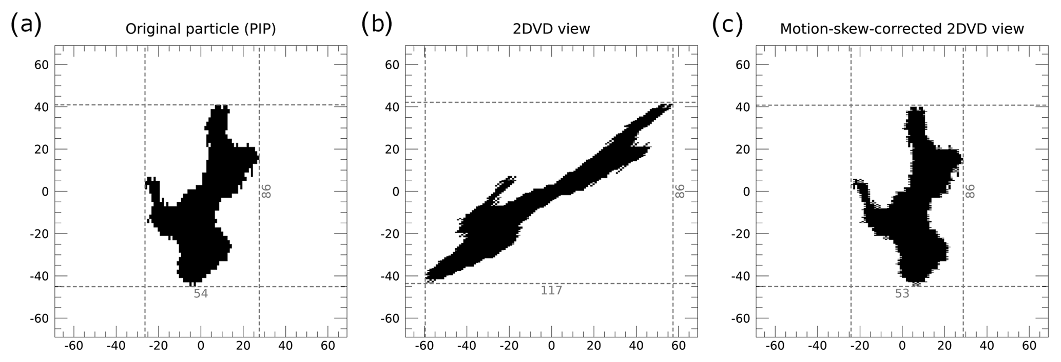
Figure 2 An example of the emulated 2DVD measurements and our unskewing algorithm including (a) the original particle as captured by the PIP camera, (b) the emulated 2DVD view of the particle before the skew correction, and (c) the emulated 2DVD view of the particle after applying our skew correction. The coordinates are in units of PIP pixels from the particle center. The dashed gray lines indicate the extent of the bounding boxes for each view of the particle, with the length of each bounding-box edge marked on the bottom and right edges in units of PIP pixels.

The image skewing produced by the horizontal movement of particles, as evident in Fig. 2b, can invalidate certain 2DVD measurements. While an algorithm designed to remove these effects exists, the algorithm is, unfortunately, in the form of a proprietary software package, and, as such, its exact inner workings are unclear. That said, Kruger and Krajewski (2002) state that the algorithm works by assuming the top-most and bottom-most pixels of the particle should be vertically aligned with one another. The algorithm then skews the image in the opposite direction to a sufficient degree to place the top- and bottom-most pixels into vertical alignment. An approximation of the unskewing algorithm has been applied to the particle in Fig. 2c; this approximation of the unskewing algorithm is described in Sect. 4.2.

4 Method

The ideal method for comparing the measurements made of snowflakes by each of these three instruments would be to have all three instruments measure the same particles simultaneously. Due to the construction of each of these instruments, however, this is not physically possible. Instead, the algorithms used by each instrument to determine particle shape will be analyzed by emulating each instrument's analysis algorithms using PIP-recorded images as an input. PIP images are used as the basis of the measurement emulation rather than MASC images because the PIP captures considerably more particles in its sampling volume than MASC does.

The PIP images used for this study come in the form of Audio Video Interleave (AVI) video files. PIP produces these video files every 10 min, and each video file contains the first 2000 frames in which PIP identified a particle during that 10 min period. If fewer than 2000 frames contained particles during a given 10 min period, the video file will contain fewer than 2000 frames. A description of how we emulate the MASC and 2DVD observations is provided in Sect. 4.1 and 4.2, and an overview of the method by which we process the PIP AVI video files in order to apply our emulated algorithms is presented in Appendix B. Additionally, we will test and evaluate an alternative ellipse-fitting method, which employs a mass tensor and is hereafter referred to as the tensor method, for retrieving particle length and width from the PIP images; this method is described in Sect. 4.3.

Ideally, we would include all PIP images from the 7–8 March 2018 period in our study rather than just those images that are included in the AVI files. Since the raw PIP image files are archived and contain every frame with precipitation, this is theoretically possible. That said, due to the very high data rates involved with the PIP data, the processing code would need to be highly optimized or use specialized software packages in order to process even a couple days of the raw data in a reasonable time frame. Thankfully, the AVI files contain a sufficiently large collection of precipitation particles to enable us to perform our study.

For the emulation of both MASC and 2DVD as well as the implementation of the tensor method, the PIP images taken from the AVI files undergo image processing matching that of the PIP (Newman et al., 2009; Larry Bliven, personal communication, 2022) prior to performing any emulation or shape fitting. First, the 8-bit image is passed through a Prewitt edge detection filter, and the results are thresholded such that all pixels with a value of at least 26 are assigned a value of 1, and all other pixels are assigned a value of zero. This 2-bit image is then dilated twice using a 3-pixel by 3-pixel kernel where all elements are set to 1. At this point, all interior holes are filled with values of 1, and the resulting 2-bit image is eroded three times using the same kernel as was used in the dilation step. The particles in the resulting image are composed of pixels that have a value of 1.

After the image processing, particles are located by matching the particle pixels to the particle positions, as identified in the PIP data files, using a region grow approach, whereby a coherent region is grown from a single point by checking its eight neighboring pixels for inclusion in the region and then repeating the process with each newly included pixel. The region grow approach is initially attempted at the PIP-determined particle centroid. For some particles with large concave regions, the PIP-measured particle center can correspond to a non-particle pixel. In these instances, an attempt is made to locate a new starting pixel for the region grow technique by searching the following (x, y) coordinate offsets in the given order: (−1, 0), (1, 0), (0, 1), (−1, 1), (1, 1), (0, −1), (−1, −1), (1, −1). If a particle pixel is not located at any of these center offset positions, the process is repeated after multiplying the offsets by a factor of 2; in cases where a particle pixel remains elusive, the process is repeated with multiples of 3 and then 4. If no particle pixels are located after checking these 32 offset positions, the particle is considered invalid and is ignored. Additionally, only particles that appear both in the particle tables (i.e., the PIP files ending in “_a_p.dat”) and in one of the two velocity tables (i.e., the PIP files ending in either “_a_v_1.dat” or “_a_v_2.dat”) are considered here as the variables contained in these files are necessary when performing the emulations.

4.1 MASC emulation

Our emulation of the MASC processing algorithm is based on the algorithm used for the US Department of Energy Atmospheric Radiation Measurement (ARM) program MASC instruments (Stuefer and Bailey, 2016; Shkurko et al., 2016). Because both the PIP and MASC ultimately perform their measurements using two-dimensional images, no special processing is performed to prepare the images before emulating the MASC measurements beyond what is described above. The emulation of the actual measurements is performed using the same ellipse fitting function as is used by the ARM MASC instrument algorithm, specifically the fitEllipse function from the OpenCV Python package (see Sect. 3.2). Although the MASC cameras have a considerably higher resolution than the PIP camera, it is worth noting that the effects of the camera resolution difference are expected to be negligible in terms of emulating the MASC shape fitting. One exception to this is that the fitEllipse function effectively requires at least 5 pixels within the target particle; for the actual MASC measurements, this represents a particle far smaller than the threshold-minimum-measured size of 0.1 mm. In the case of the emulated MASC, a 5-PIP-pixel particle would have an area of 0.5 mm² and a maximum dimension of at least 0.3 mm as the PIP pixels are calibrated to be 0.1 mm on each side. To avoid having particles that can only be analyzed by a subset of the shape-fitting algorithms, our comparisons here will only consider particles which have an equivalent area of at least 0.5 mm².

4.2 2DVD emulation

The 2DVD instrument captures a series of one-dimensional images as a particle falls through the observing volume. As such, the PIP images must be resampled in a way that mimics the 2DVD instrument itself. To this end, we use snapshots of the PIP-observed particles and replicate the horizontal and vertical motions of the particles, as measured by PIP, using bilinear interpolation. The vertical motion is replicated by shifting the vertical coordinates of the bilinear interpolation upward by an amount equal to the particle fall speed divided by the camera observation frequency; for 2DVD, the camera observation frequency is 68 200 Hz. The horizontal motion is replicated by shifting the particle snapshot pixel locations horizontally in the direction of particle motion by an amount equal to the distance traveled by the particle during the elapsed time of the emulated observations, to the nearest 0.1 mm. This elapsed time is equal to the product of the inverse of the camera observation frequency and the number of times the particle has been sampled in the vertical up until that point (i.e., the number of emulated 2DVD line scans performed). When performing the interpolations, only the interpolated pixels with a value of 1 are considered part of the emulated 2DVD observation.

An example of an emulated 2DVD observation is depicted in Fig. 2 with the original, PIP-observed, particle image depicted in Fig. 2a and the emulated 2DVD particle image depicted in Fig. 2b. Note the considerable skewing that has occurred in the emulated 2DVD image relative to the PIP image due to the horizontal movement of the particle towards the left as it passed through the virtual line-scan camera. As previously mentioned, 2DVD applies an unskewing algorithm to correct for the distortions introduced by the horizontal motion of the particle. Because this algorithm is part of a proprietary software package and not openly available, we have chosen to approximate the effects of the algorithm based on the conceptual description provided by Kruger and Krajewski (2002).

Recall, from Sect. 3.3, that the 2DVD unskewing algorithm works by assuming that the top-most and bottom-most points on an observed particle are actually vertically aligned with one another (Kruger and Krajewski, 2002). In the event of multiple particle pixels appearing on the top-most or bottom-most scan line, it is unclear how the actual algorithm selects the top-most or bottom-most point of the particle. To this end, we have decided to define the top-most and bottom-most points of the particle as the mean horizontal location of the particle pixels on the top-most and bottom-most scan lines, respectively.

The actual unskewing process in our algorithm works by linearly interpolating the horizontal offset, as implied by the motion-skewed locations of the top-most and bottom-most points of the particle, to the vertical position of each scan line. Each scan line is then horizontally shifted by the appropriate offset via another linear interpolation. The value of the interpolated pixels is then rounded to either zero, indicating a non-particle pixel, or 1, indicating a particle pixel. Figure 2c depicts the result of applying the unskewing algorithm; note the slight differences in the apparent particle orientation between the original image (Fig. 2a) and the unskewed image (Fig. 2c). We will examine the effects of these differences on the accuracy of the 2DVD bounding-box measurements in Sect. 5.2.

4.3 Tensor method

To provide an additional point of comparison for the particle measurements, we also implemented an alternative ellipse fitting strategy, referred to here as the tensor method, that uses the method implemented in the fit_ellipse program in the Coyote IDL Library (http://www.idlcoyote.com, last access: 14 November 2022). This method works by computing the eigenvalues, e₁ and e₂, of a two-by-two mass distribution tensor matrix, which is defined as

$$\begin{array}{}\text{(1)}& \mathit{\tau }=\left[{\displaystyle \frac{(\stackrel{\mathrm{‾}}{\mathrm{\Delta }y){}^{\mathrm{2}}}}{\mathrm{\Delta }x\mathrm{\Delta }y}}{\displaystyle \frac{\stackrel{\mathrm{‾}}{\mathrm{\Delta }x\mathrm{\Delta }y}}{\left(\mathrm{\Delta }y\right){}^{\mathrm{2}}}}\right],\end{array}$$

where Δx and Δy are the distances from the particle centroid in the horizontal and vertical directions, respectively, and the overbars indicate averaging. The semimajor and semiminor axes, a and b, respectively, are then calculated from the eigenvalues via

$$\begin{array}{}\text{(2)}& a=\mathrm{2}\sqrt{e_{\mathrm{1}}}\mathrm{and}b=\mathrm{2}\sqrt{e_{\mathrm{2}}}.\end{array}$$

The major and minor axes of the fitted ellipse can then be obtained simply by doubling the semimajor and semiminor axes. Finally, in the interest of completeness, the tensor-fitted ellipse orientation, measured counterclockwise from the positive x axis, is computed as $\left(e_{\mathrm{2}}/e_{\mathrm{1}}\right)-\mathrm{90}{}^{\circ }$. As will be discussed in Sect. 5.1, the tensor method produces similar, although not identical, fits to those of the emulated MASC method.

5 Results

5.1 MASC and PIP shape-fitting measurements

As discussed in Sect. 4, the PIP data for the period between 00:00 UTC on 7 March and 00:00 UTC on 9 March 2018 at the ICE-POP MHS observation site were processed using algorithms designed to emulate both the MASC and 2DVD measurements of particle dimension. The present section will focus on the measurements made using the MASC and PIP shape-fitting methods as well as the tensor method. A comparison of the bounding-box measurement techniques used by PIP and 2DVD will be the subject of a separate section (Sect. 5.2) rather than being included here. Although the tensor-fitted ellipse measurements will be used here as a point of comparison between the various instrument algorithms, it should be noted that the tensor-fitted ellipse measurements are not a “ground truth” and are subject to errors of their own.

Comparing the PIP-fitted ellipse particle dimensions to those of the tensor-fitted ellipse, we found that the PIP-fitted ellipse tends to overestimate the long dimension of the particle (Fig. 3a), measured as the major axis of the fitted ellipse, and underestimate the short dimension (Fig. 3d), measured as the minor axis of the fitted ellipse, relative to the tensor-fitted ellipse. As a result, the aspect ratio, computed as the short dimension divided by the long dimension, is almost always underestimated by the PIP-fitted ellipse relative to the tensor-fitted ellipse. This underestimation is particularly noticeable for larger tensor-fitted ellipse aspect ratios, with the PIP-fitted ellipse aspect ratio rarely exceeding 0.6 and never reaching 0.7 during this event, despite there being a period of lump graupel, which should have a relatively high aspect ratio due to its almost spherical shape, on 8 March (Fig. 4a). This effectively represents an artificial cap in PIP-fitted ellipse aspect ratio.

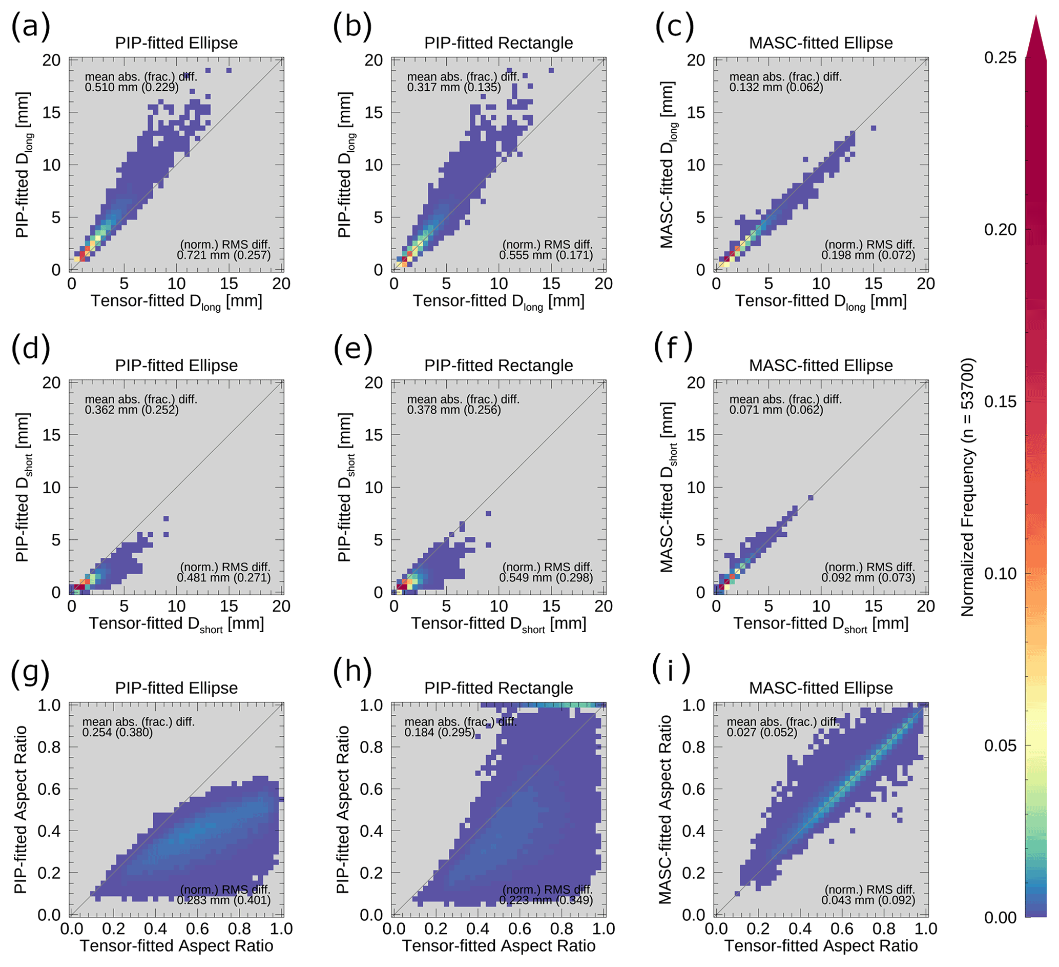
Figure 3 Two-dimensional histograms of (a–c) particle long dimension (in mm), (d–f) particle short dimension (in mm), and (g–i) particle aspect ratio for (a, d, g) the PIP-fitted ellipse, (b, e, h) the PIP-fitted rectangle, and (c, f, i) the emulated MASC-fitted ellipse as a function of the tensor-fitted ellipse values. The diagonal gray lines indicate where the x value is equal to the y value. The mean absolute difference and root-mean-square difference for each pair of measurements are indicated in each panel, with the mean absolute fractional difference and normalized root-mean-square difference in parentheses. Only particles with a PIP-measured area greater than 0.5 mm² are included. Note that a logarithmic color table has been used to highlight the frequency distribution at lower values.

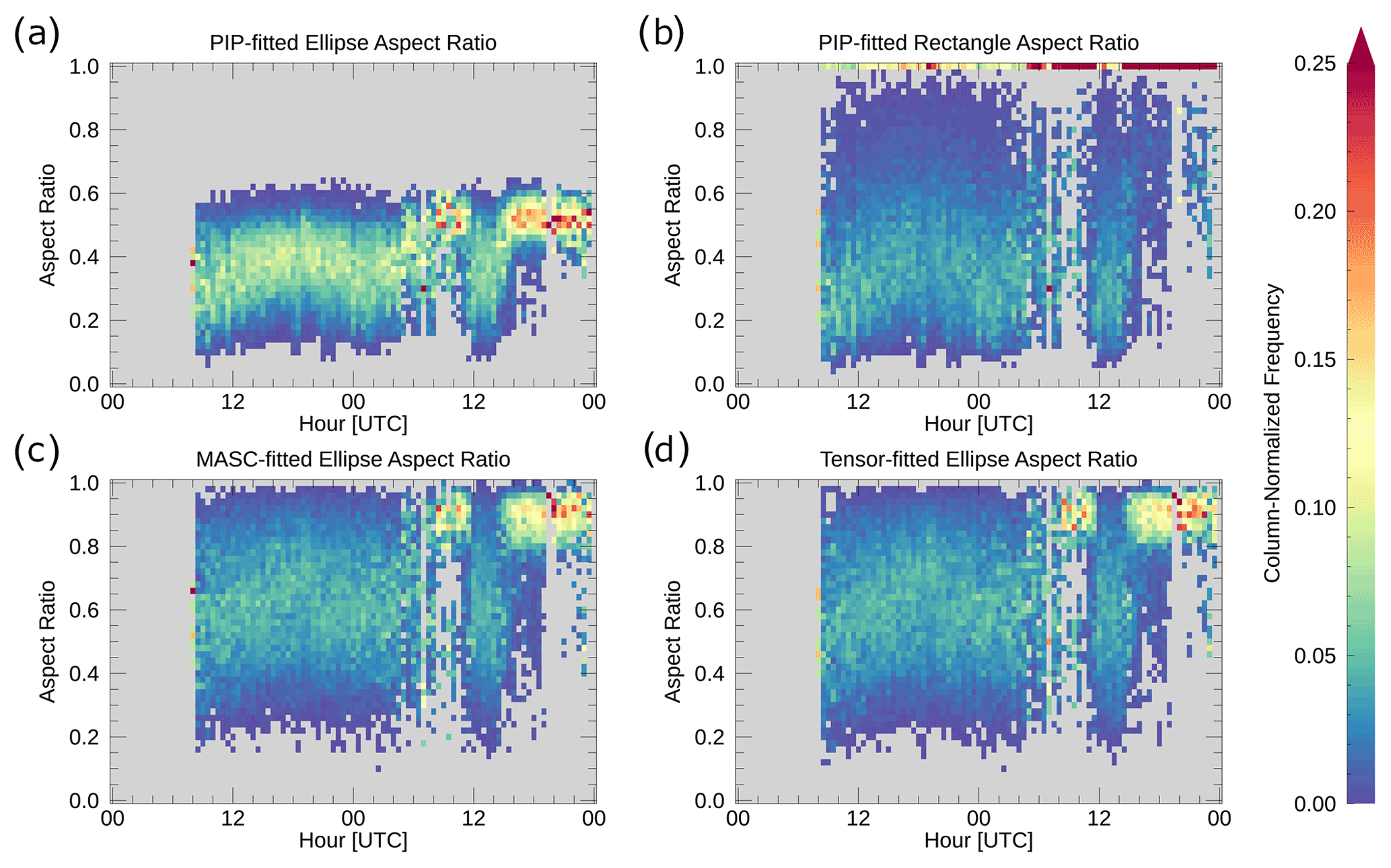
Figure 4 Time series of the (a) PIP-fitted ellipse, (b) PIP-fitted rectangle, (c) emulated MASC-fitted ellipse, and (d) tensor-fitted ellipse aspect ratio distributions for the 7–8 March 2018 case. Only particles with an area of at least 0.5 mm² were included in the histograms. The bin counts of each column have been normalized such that they add up to 1.

Using the PIP-fitted rectangle as the basis of the particle dimension measurements produces a sizable improvement to the agreement between the PIP-fitted long dimension and the tensor-fitted long dimension (Fig. 3a and b) but almost no change in agreement for the short dimension (Fig. 3d and e). To quantify these changes in the dimension measurement agreement, we use both the mean absolute difference, defined as the average magnitude of the difference between two sets of measurements, and the mean absolute fractional difference, defined as the average magnitude of the normalized difference between two sets of measurements; for Fig. 3, the normalization is done relative to the measurements made using the tensor method. Comparing the mean absolute differences for the PIP-fitted ellipse and PIP-fitted rectangle dimensions, the PIP-fitted rectangle long dimension has a mean absolute difference from the tensor-fitted long dimension that is approximately three-fifths that of the PIP-fitted ellipse long dimension (Fig. 3a and b). The PIP-fitted ellipse and rectangle short dimensions, however, show almost no change in mean absolute difference (Fig. 3d and e).

In terms of aspect ratios, the PIP-fitted rectangle aspect ratio (Fig. 3h) does not suffer from the artificial cap that was present with the PIP-fitted ellipse aspect ratio (Fig. 3g), and much of the reduction in the mean absolute difference (0.254 versus 0.184) is likely tied to the lack of said artificial cap. That said, the PIP-fitted rectangle aspect ratio still has a tendency to greatly underestimate the aspect ratio relative to the tensor-fitted ellipse aspect ratio (Figs. 3h, 4b and d). In contrast to the PIP-fitted ellipse aspect ratios, the PIP-fitted rectangle aspect ratio does capture the large aspect ratios associated with the periods of lump graupel precipitation on 8 March around 09:00 UTC and after 14:00 UTC, although these aspect ratios are almost entirely reported as a value of 1. Interestingly, the PIP-fitted rectangular aspect ratio frequently has a value of 1 but very rarely has a value between 0.9 and 1; this peculiarity will be revisited later in this section.

In contrast to the two sets of PIP-fitted measurements, the MASC-fitted ellipse measurements show very good agreement with the tensor-fitted ellipse measurements of both the long and short dimension of the fitted particles (Fig. 3c and f), with mean absolute differences ranging between approximately one-fifth and two-fifths those for the PIP-fitted shapes. As a result, the aspect ratios computed from shapes fitted using the emulated MASC method and the tensor method are in fairly good agreement as well (Fig. 3i). This general agreement between the particle dimensions measured from the MASC-fitted and tensor-fitted ellipses suggests that these two shape-fitting algorithms may give more reliable results than the PIP-fitted ellipse or rectangle algorithms. To gain insight into whether the MASC and tensor method algorithms are, in fact, performing better than the PIP algorithms, we will take a closer look at individual particles.

Figure 5a–d depict snapshots of particles taken from the PIP AVI files with the fitted shapes from the various fitting algorithms depicted in Fig. 5e–h. For simplicity, these particles will be referred to by the Fig. 5 panel letter of the unannotated panels (i.e., panels a–d). Particles (a) and (b) are both likely some type of aggregate frozen precipitation based on their odd shapes. Based on the relatively circular shapes of the remaining two particles, relatively high fall speeds (black line, Fig. 1), subfreezing near-surface temperatures (red line, Fig. 1), and the lack of an above-freezing temperature layer in a nearby thermodynamic sounding (not shown), particles (c) and (d) are likely both examples of lump graupel. Qualitative and quantitative inspection of the particles in Fig. 5 and Table 1 supports the patterns identified by the scatter-plot analysis performed above. Specifically, the PIP-fitted ellipse appears to always overestimate the particle long dimension; the PIP-fitted rectangle appears to sometimes overestimate, sometimes underestimate, and sometimes accurately capture the particle long dimension; and, finally, the emulated MASC-fitted and the tensor-fitted ellipses tend to produce fairly similar particle dimensions. Additionally, visual examination of these and other (not shown) individual particles suggests that the emulated MASC-fitted and the tensor-fitted ellipses tend to provide more reasonable estimates of particle dimension than either of the PIP-fitted shapes.

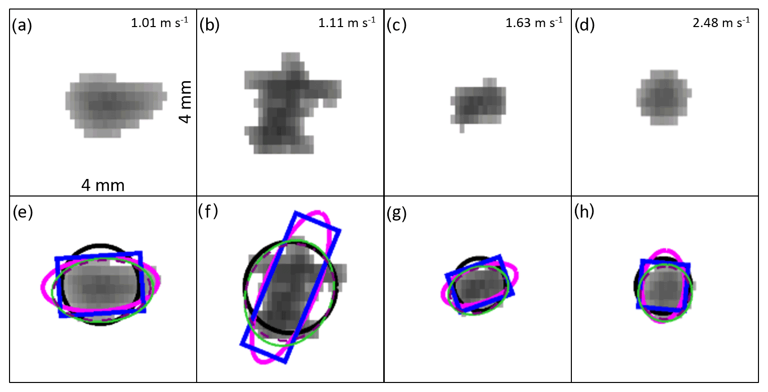
Figure 5 Snapshots of four particles as viewed by PIP, displayed (a–d) without shape annotations and (e–h) with shape annotations. The images were captures at approximately (a, b, e, f) 19:04 UTC on 7 March 2018 and (c, d, g, h) 17:56 UTC on 8 March 2018. Fall speeds are listed in the top right corner of (a)–(d); the fall speeds for particles (a) and (b) are computed by PIP, while the fall speeds for particles (c) and (d) are manually calculated as the average frame-to-frame center position motion as these specific particles were not included in the PIP particle velocity files. The shape annotations in (e)–(h) include (black) the area-equivalent circle, (magenta) the PIP-fitted ellipse, (blue) the PIP-fitted rectangle, (dashed purple) the emulated MASC-fitted ellipse, and (green) the tensor-fitted ellipse. Each panel represents a square that is 4 mm long on each side. The dimensions of the fitted shapes for each particle are presented in Table 1.

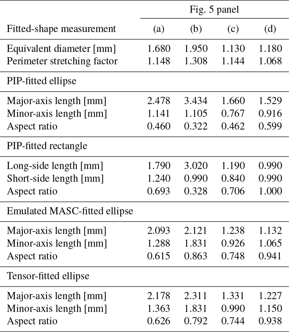
Table 1 Dimensions and aspect ratios of the fitted shapes for various particle fits depicted in Fig. 5, referenced by the figure panel letter for the unannotated particle images. The perimeter stretching factor is computed by dividing the actual particle perimeter by the perimeter of a circle of equal area to the particle.

The primary cause of the discrepancies between the actual particle shape and the PIP-fitted ellipse major and minor axes is rooted in the reliance on only the particle area and perimeter for making the PIP fits, as discussed in Sect. 3.1. For particles with complicated outlines, such as particle (b), the particle perimeter is far greater than the perimeter of an ellipse or rectangle of equal dimensions (i.e., length and width). To make up the extra perimeter for a given area, the PIP-fitted ellipse or rectangle must have a larger long dimension at the expense of the short dimension.

The relationship between excess perimeter for a given area, relative to a perfect ellipse, and error in the PIP-fitted-ellipse or rectangle-dimension lengths is demonstrated in Fig. 6 for a hypothetical particle that we will assume is generally circular with a mean radius of 0.5 mm but whose edge is not a perfect circle and is allowed to vary about the mean radius of 0.5 mm in such a way that the area and center position remain unchanged from that of a 0.5 mm radius circle. The amplitude of this variation in radius is represented in Fig. 6 by the perimeter stretching factor, computed as the actual perimeter of a particle divided by the perimeter of a circle of equal area to the particle. A perimeter stretching factor of 1 will result in a perfect circle, while a larger perimeter stretching factor indicates the presence of larger variations in radius (i.e., a more complicated shape). For our hypothetical particle, we prescribe a value between 1 and 2 for the perimeter stretching factor and set the particle area to be equal to that of a 0.5 mm radius circle. As the PIP-fitting method only requires perimeter and area, our parameterization of the hypothetical particle is sufficient to perform an ellipse or rectangle fit without constructing the hypothetical particle itself. The equations used to make the PIP fits are derived in Appendix A. Note that nothing in these equations relates to the actual shape of the particle itself (e.g., with or without concave regions); this missing information is, in fact, the core issue with both the PIP ellipse and rectangle fits. Without knowledge of the underlying distribution of pixels within the particle, the PIP algorithm assumes all particles are either smooth-edged ellipses or rectangles, depending on which fit is used.

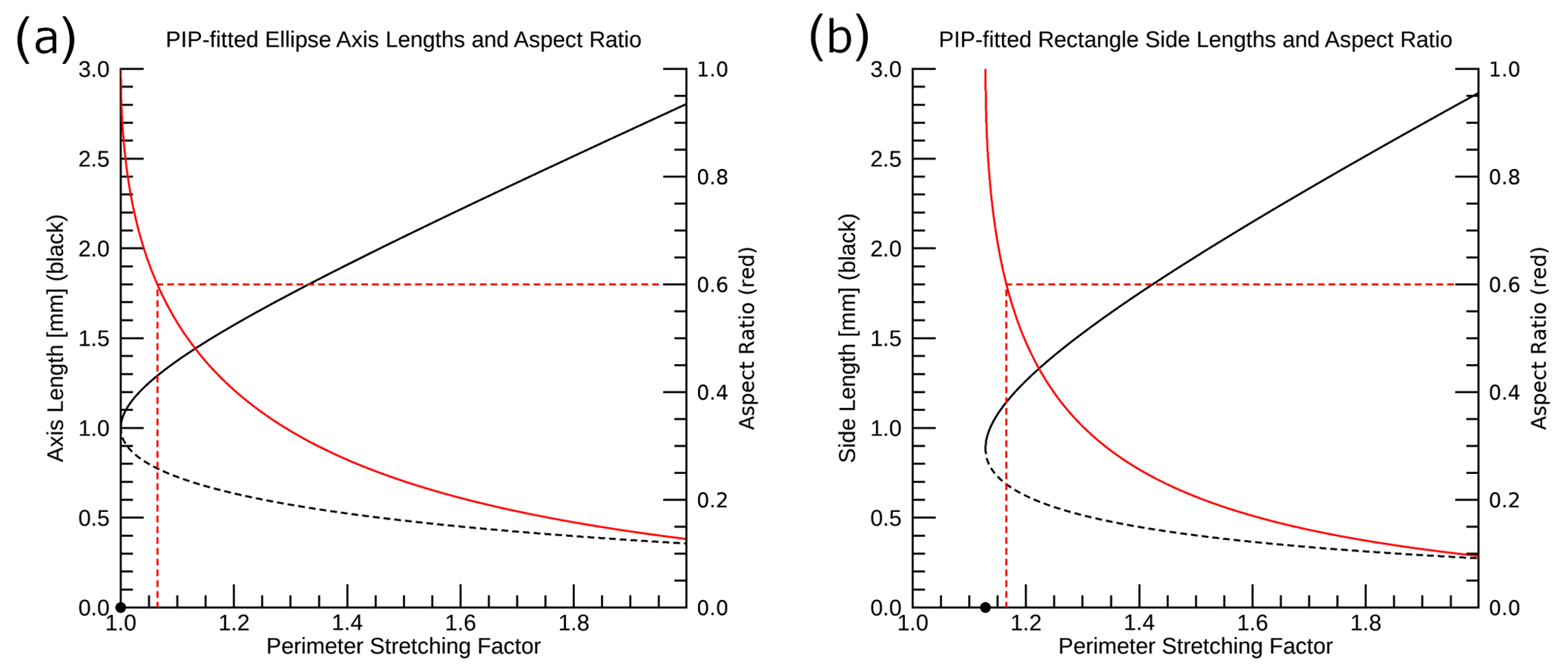
Figure 6 Demonstration of the impact of excess perimeter for a given area on the (a) PIP-fitted ellipse and (b) PIP-fitted rectangle long-axis length (solid black), short-axis length (dashed black), and aspect ratio (solid red). This example uses a circle with a radius of 0.5 mm to compute the base perimeter and area. The dashed red lines highlight the perimeter stretching factor that corresponds to an aspect ratio of 0.6, and the black dot on the x axis indicates the minimum perimeter stretching factor for which a physically meaningful shape can be fitted.

The lack of shape information in the PIP shape-fitting equations does not entirely explain the artificial cap in aspect ratio at ∼0.6 for the PIP-fitted ellipses (as in Figs. 3g and 4a), however. If the shape issues were the sole cause of the artificial cap, the circular presentation of particle (d) in Fig. 5 would produce a very good fit with an aspect ratio approaching 1. Instead, the aspect ratio cap is a result of where the aspect ratio is most sensitive to the perimeter length for a given particle area. Based on Fig. 6a, the PIP-fitted ellipse major and minor axis lengths and aspect ratio show the greatest sensitivity to perimeter length when the perimeter stretching factor is almost 1 (i.e., the particle is almost a perfect circle). As a result, any deviation from the smooth edge of a perfect circle will produce relatively rapid changes in the ellipse axis lengths and the aspect ratio. It was noted above that the PIP-fitted ellipse measurements (Fig. 4a) appear to produce an artificial cap on aspect ratio of approximately 0.6. Based on our calculations for Fig. 6, a PIP-fitted ellipse aspect ratio of 0.6 is produced when the perimeter stretching factor is approximately 1.065, regardless of the actual shape of the particle. For reference, a perimeter stretching factor of 1.065 corresponds to taking a 10 mm diameter circular particle, which would have a perimeter of ∼31.4 mm, and stretching its perimeter by 2 mm. Small increases in perimeter, such as this, can be introduced by a few very small deviations of the true particle edge from a perfect circle as well as by the inability to perfectly represent a circle using square pixels (i.e., pixelation effects).

The PIP-fitted rectangle long- and short-side lengths (Fig. 6b) have a similar sensitivity to changes in perimeter stretching factor when the perimeter stretching factor is relatively small. A key difference from the PIP-fitted ellipses, however, is that a rectangle cannot be fit to a particle whose perimeter stretching factor is less than $\sqrt{\mathrm{4}/\mathit{\pi }}$ (∼1.128), below which the particle perimeter is not long enough to construct a rectangle of the required area. Particle (d) in Fig. 5 is an example of a particle whose perimeter is too short to produce a physical rectangle fit using the PIP method. The perimeter stretching factor for particle (d) is approximately 1.068, as listed in Table 1. Based on this and similar particles, the PIP processing algorithm appears to automatically assign an aspect ratio of 1 to any particle where a rectangle fit is not physically possible, the effects of which can be seen in Fig. 4b. How the PIP algorithm determines a dimension length in these cases, however, remains unclear.

The artificial cap in aspect ratio that appears for the PIP-fitted ellipses (Fig. 4a) does not appear to be present in the aspect ratio distributions for the PIP-fitted rectangles (Fig. 4b). A key factor that leads to this difference is demonstrated in Fig. 6b: a rectangle aspect ratio of 0.6 corresponds to a perimeter stretching factor of ∼1.165 compared to 1.065 for a PIP-fitted ellipse (Fig. 6a). The importance of this perimeter stretching factor difference of 0.1 comes down to the observed distribution of particle perimeters relative to their areas (i.e., the distribution of particle stretching factors). Figure 7 depicts the distribution of observed perimeter stretching factors for the 7–8 March 2018 case. Only a very small portion of particles have a perimeter stretching factor smaller than 1.065 (left dashed red line, Fig. 7), whereas the most frequently observed perimeter stretching factors are smaller than the 1.165 perimeter stretching factor (right dashed red line, Fig. 7) that corresponds to the 0.6 aspect ratio for a PIP-fitted rectangle.

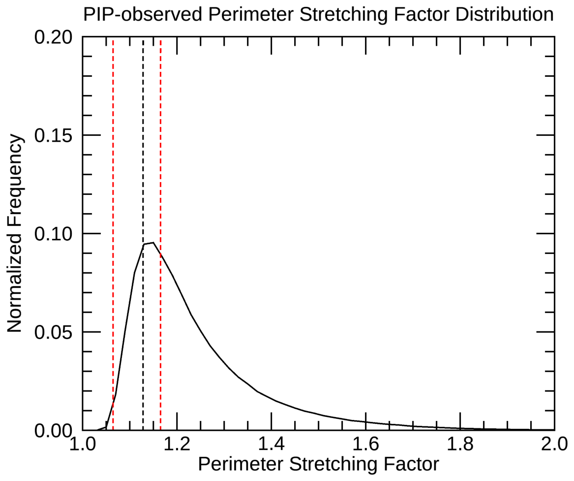
Figure 7 Distribution of perimeter stretching factors computed from PIP observations collected during the 7–8 March 2018 snow event. The two vertical dashed red lines indicate the perimeter stretching factor corresponding to an aspect ratio of 0.6 for (left dashed red line) a PIP-fitted ellipse and (right dashed red line) a PIP-fitted rectangle. The vertical dashed black line indicates the smallest perimeter stretching factor that will permit a physically meaningful rectangle fit. Only particles with an area of at least 0.5 mm² are included in the histogram.

5.2 2DVD and PIP bounding-box measurements

Because the 2DVD does not instantaneously capture full images of a particle, a “long-dimension versus short-dimension” aspect ratio is not computed by the instrument. Instead, 2DVD reports the “oblateness” of a particle, defined as the aspect ratio of the horizontal width of a particle versus its vertical height. For each camera, the oblateness is computed as the bounding-box height divided by the bounding-box width. An overall oblateness is then computed from the two single-camera oblateness values by their geometric mean. Here we will focus on the measurements of the bounding-box height and width rather than the oblateness itself.

Both PIP and 2DVD record measurements of the horizontal and vertical extent of a particle in the form of bounding-box measurements, computed as the horizontal distance between the left-most and right-most particle pixels and the vertical distance between the bottom-most and top-most particle pixels. Because PIP takes measurements using two-dimensional images, the accuracy of the PIP bounding-box measurements is directly tied to camera resolution, motion blurring effects, and image compression effects. 2DVD, however, uses a line-scan camera, and, as such, the 2DVD bounding-box measurements are derived quantities. The bounding-box height is derived from the time required for the particle to pass through the sampling region, while the bounding-box width is computed by compositing the individual line scans to rebuild the particle. As discussed in Sect. 3.3, 2DVD uses an unskewing algorithm to correct the bounding-box-width measurements for horizontal particle motion. As the actual 2DVD unskewing algorithm is part of a proprietary software package, we use a conceptually similar unskewing algorithm, described in Sect. 4.2.

The vertical sampling frequency of the emulated 2DVD images is usually much higher than that of the underlying PIP images due to the high temporal sampling frequency of 2DVD. In order for the vertical sampling frequency of the emulated 2DVD images to be lower than that of the underlying PIP images, the precipitation particle would need to have a fall speed greater than ∼68.2 m s⁻¹, which is unrealistic for any of the particles of interest. Because of this, we would expect the emulated 2DVD bounding-box height to almost exactly match the PIP-measured bounding-box height, and this expectation is borne out: the mean absolute difference between the PIP and 2DVD bounding-box heights (not shown) is only 0.016 mm (a mean absolute fractional difference of 0.013).

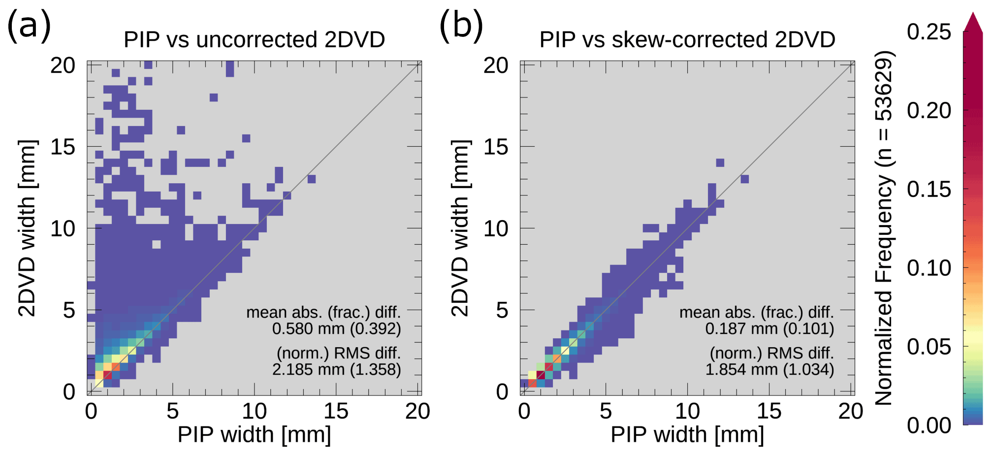
Figure 8 Two-dimensional histograms comparing the PIP bounding-box width to the emulated (a) uncorrected and (b) skew-corrected 2DVD bounding-box width. The mean absolute difference and root-mean-square difference for each pair of measurements are indicated in each panel, with the mean absolute fractional difference and normalized root-mean-square difference in parentheses. Only particles with a PIP-measured area of at least 0.5 mm² are included in the plots. Note that a logarithmic color table has been used to highlight the frequency distribution at lower values.

Of greater interest is how well the emulated 2DVD bounding-box-width measurements perform, especially after we apply our approximation of the 2DVD unskewing algorithm. Figure 8a compares the uncorrected emulated 2DVD bounding-box width with the PIP-measured bounding-box width. Unsurprisingly, the uncorrected 2DVD measurements tend to greatly overestimate the width of the bounding box due to the skewing introduced by any horizontal motion of the particle. One point of interest, however, is that the uncorrected 2DVD measurements can sometimes underestimate the bounding-box width. This can occur when a particle of sufficiently low aspect ratio is moving in the opposite direction of the tilt of the top of the particle (e.g., a needle crystal whose top is to the left of the particle centroid moving towards the right); this will result in the particle being compressed in the horizontal because the particle is scanned from the bottom upwards as it falls through the plane of the line-scan camera.

Despite the complex shapes attributed to snowflakes, the emulated 2DVD measurements of bounding-box width are surprisingly accurate once our approximation of the 2DVD unskewing algorithm is applied (Fig. 8b). Quantitatively, the unskewing algorithm produces a reduction in mean absolute difference from 0.58 to 0.187 mm. After the correction, the overestimation of bounding-box width is considerably reduced compared to the uncorrected emulated 2DVD measurements. The underestimation of bounding-box width that was present with the uncorrected measurements, however, is more common after the correction. The increase in underestimation is due to the assumption that the top-most and bottom-most pixels of the 2DVD-imaged particle are supposed to be vertically aligned with one another. This assumption is frequently broken by snow particles, leaving the 2DVD measurements of snowflake horizontal extent potentially unreliable in comparison to PIP. An example of this assumption resulting in a very minor underestimation of bounding-box width can be seen in Fig. 2.

6 Discussion

Previous studies have examined a number of error sources that impact the accuracy of optical disdrometer measurements. To better understand the magnitude of the differences examined in the present study, it is worth a brief comparison to the findings of past studies.

Simulating two-dimensional observations of three-dimensional particles for the SVI (the predecessor of PIP) and 2DVD, Wood et al. (2013) found that, under reasonable conditions, using a two-dimensional projected long-dimension length would result in the observed long dimension being approximately 82 % of the actual particle long dimension, thereby underestimating reflectivity by 3.2 dB. Using three-dimensional snowflake replicas, Leinonen et al. (2021) determined that the two-dimensional measurements of particle long dimension made by MASC have a normalized root-mean-square error of ∼6 % relative to the actual particle long dimension. Leinonen et al. (2021) only examined measurements of snowflakes with a long dimension between 3 and 5 mm, and the study used the largest long dimension measured among the three MASC cameras rather than using a single-camera measurement. By comparison, we found the normalized root-mean-square difference between the long dimension of the tensor-fitted ellipse and the PIP-fitted ellipse, PIP-fitted rectangle, and MASC-fitted ellipse to be ∼26 %, ∼17 %, and ∼7 %, respectively, and these numbers do not change by much when only particles with a tensor-fitted ellipse long dimension between 3 and 5 mm are included in the calculation. This suggests that the PIP shape-fitting issues have a much greater impact on the determination of the particle long dimension than the loss of information caused by projecting a three-dimensional snowflake into a two-dimensional view does. Interestingly, it also suggests that differences between the MASC-fitted ellipse and tensor-fitted ellipse are slightly larger than the error introduced using the two-dimensional projection of the particle to measure long-dimension length, although this could be due to Leinonen et al. (2021) using the maximum long dimension from among the three MASC cameras rather than just using a single camera.

7 Conclusions

The present study set out to evaluate the measurement techniques used by PIP, MASC, and 2DVD to characterize the shape of snowflakes in terms of their aspect ratio, which is computed as the ratio of the particle short-dimension length to the particle long-dimension length. This was accomplished using imagery collected by a PIP instrument during the ICE-POP 2018 field campaign to emulate the relevant measurements made by MASC and 2DVD. More specifically, a comparison was made between the ellipse- and rectangle-fitting algorithms used by PIP and the ellipse-fitting algorithm used by MASC; a tensor-based ellipse-fitting algorithm was also evaluated alongside the PIP and MASC shape-fitting algorithms. Additionally, measurements of the bounding-box width and height made by PIP were compared to the emulated 2DVD width and height measurement in order to evaluate the performance of 2DVD when measuring snow particles. The key findings of our comparative evaluation are listed below.

• The MASC ellipse-fitting algorithm produces reasonable ellipse fits of the particles and, as such, produces reliable aspect ratios (Sect. 5.1).

• The PIP shape-fitting algorithms do not perform well due to their reliance on only the area and perimeter of a particle, leading to a tendency towards overestimating the long dimension and underestimating the short dimension (Sect. 5.1).

• The aspect ratios of the PIP-fitted shapes are highly sensitive to small deviations from the smooth-edged fitted shape, such as pixelation effects or any underlying non-sphericity of the particles (Sect. 5.1).

• The tensor method performed comparably to the MASC ellipse-fitting algorithm (Sect. 5.1).

• Our implementation of the 2DVD unskewing algorithm, designed to remove the effects of horizontal motion from the 2DVD bounding-box-width measurements, performed surprisingly well with snow particles considering the instrument was designed to measure raindrops. That said, the corrected bounding-box-width measurements are still prone to error due to the motion skewing effects. We expect that the actual, proprietary implementation of this algorithm would have a similar level of performance (Sect. 5.2).

These results suggest that all three instruments have potential applications for studying snow, albeit with differing degrees of effectiveness. The MASC and PIP cameras, which capture two-dimensional images directly, are better suited for measuring snowflake shape than the line-scan cameras used by 2DVD as the MASC and PIP cameras are not susceptible to the image skewing produced by the horizontal motion of a particle that is experienced by 2DVD. That said, the 2DVD skew correction was able to correct most of the skewing introduced by horizontal motion.

PIP suffers from the issue that the shape-fitting routines do not perform well on frozen precipitation particles, and, as a result, the PIP-fitted- ellipse- and rectangle-dimension (and, therefore, aspect ratio) measurements are unreliable. Worth noting, however, is that the PIP shape-fitting issues only impact four variables: “Ellip_Maj”, “Ellip_Min”, “Rec_BS”, and “Rec_SS”; the other PIP-reported measures of particle size (e.g., particle bounding-box dimensions, area, and equivalent diameter) remain reliable. As such, any products that use a non-shape-fitting measure of particle size (e.g., Pettersen et al., 2020) remain unaffected by the shape-fitting issue. As the present study has demonstrated, the PIP imagery can be reprocessed, and reliable measurements of the long dimension and aspect ratio can be made via the application of an alternative ellipse-fitting algorithm, such as the MASC or tensor-based algorithms. While not demonstrated here, it may be possible to also implement a shape-fitting algorithm for 2DVD using the reconstructed images captured by the line-scan camera, although the reliability of the resulting shape measurements from such an algorithm would need further investigation to test the impacts of the image skewing.

Appendix A: Derivation of shape-fitting equations for PIP

According to the IMAQ Vision Concepts manual (National Instruments, 2000), the equations to fit either an ellipse or a rectangle can be derived from the equations for area and perimeter. The area and perimeter equations for a rectangle are, respectively,

$$\begin{array}{}\text{(A1)}& {\displaystyle }A=ab\mathrm{and}\text{(A2)}& {\displaystyle }P=\mathrm{2}\left(a+b\right),\end{array}$$

where A is the actual particle area, P is the actual particle perimeter, and a and b are the lengths of the long and short sides of the fitted rectangle. For an ellipse, PIP uses the following equations for area and perimeter, respectively:

$$\begin{array}{}\text{(A3)}& {\displaystyle }A=\mathit{\pi }ab\mathrm{and}\text{(A4)}& {\displaystyle }P=\mathit{\pi }\sqrt{\mathrm{2}\left(a^{\mathrm{2}}+b^{\mathrm{2}}\right)},\end{array}$$

where the major axis length is equal to 2a, and the minor axis length is equal to 2b. Note that the equation that PIP uses for the perimeter of an ellipse is actually an upper bound on the perimeter of an ellipse rather than an actual estimate of the perimeter (Jameson, 2014).

The derivation for the equations used to compute the dimensions of both the PIP-fitted ellipse and rectangle proceed similarly: solving the area equation for either a or b and substituting the result into the perimeter equation. This substitution is followed by putting the resulting equation into the standard form for a quadratic equation for the rectangle and a quartic equation for the ellipse. The standard-form quadratic equation for the rectangle fit is

$$\begin{array}{}\text{(A5)}& \mathrm{0}=-x^{\mathrm{2}}+{\displaystyle \frac{P}{\mathrm{2}}}x-A,\end{array}$$

where x is either a or b depending on the variable for which the area equation was solved. Similarly, the standard-form quartic equation for the ellipse fit is

$$\begin{array}{}\text{(A6)}& \mathrm{0}=-{\mathit{\pi }}^{\mathrm{2}}{x}^{\mathrm{4}}+{\displaystyle \frac{P^{\mathrm{2}}}{\mathrm{2}}}{x}^{\mathrm{2}}-A^{\mathrm{2}}.\end{array}$$

Note that the IMAQ Vision Concepts manual incorrectly records the standard-form equation for the ellipse fit as being identical to that of the rectangle fit.

The standard-form equations for both the rectangle and ellipse fits can then be solved for their roots. As the ellipse-fit equation is a biquadratic special case of a quartic equation, it can be solved using the same method as a quadratic equation by substituting z=x², determining the roots, and then substituting $x=\pm \sqrt{z}$ into those roots. Solving both equations via the these methods gives roots of

$$\begin{array}{}\text{(A7)}& x={\displaystyle \frac{P}{\mathrm{4}}}\pm {\displaystyle \frac{\sqrt{\frac{P^{\mathrm{2}}}{\mathrm{4}}-\mathrm{4}A}}{\mathrm{2}}}\end{array}$$

for the PIP-fitted rectangle and

$$\begin{array}{}\text{(A8)}& x=\pm \sqrt{{\displaystyle \frac{P^{\mathrm{2}}}{\mathrm{4}{\mathit{\pi }}^{\mathrm{2}}}}\pm {\displaystyle \frac{\sqrt{\frac{P^{\mathrm{4}}}{\mathrm{4}}-\mathrm{4}{\mathit{\pi }}^{\mathrm{2}}{A}^{\mathrm{2}}}}{\mathrm{2}{\mathit{\pi }}^{\mathrm{2}}}}}\end{array}$$

for the PIP-fitted ellipse. The only physically meaningful roots will be the positive roots. In the case of the quartic ellipse equation, one of the positive roots will give the value of a, and the other will give the value of b. The other dimension for the rectangle fit can be computed by plugging the positive root into the equation for area and solving for the unknown dimension length (either a or b).

Appendix B: PIP video file processing

The following builds on Sect. 4 by further discussing the steps taken to reprocess the PIP video files in order to produce the emulated MASC and tensor method fits as well as the emulated 2DVD measurements. Reprocessing the PIP video files for the alternative fits requires four sets of files: the AVI video files, the _a_p.dat particle table files, the _a_v_1.dat velocity table files, and the _a_v_2.dat velocity table files. The two velocity table files cover different sets of particles: the _a_v_1.dat files contain data for particles that were only observed in two consecutive frames, while the _a_v_2.dat files contain data for all particles that were observed in three or more consecutive frames. Using both files maximizes the number of particles that we can use to make emulated 2DVD measurements. Each AVI file corresponds to one of each of the `.dat' files, although the “.dat” files typically cover a much greater period of time than what is depicted in the AVI files. The key “.dat” file variables for the reprocessing algorithm are listed in Table B1.

Table B1 List of relevant variables within PIP data files for reprocessing the PIP AVI video files.

The PIP AVI videos include both the PIP view as well as a header that indicates which PIP unit recorded the observations, the time stamp, a combined “Q_R” frame index, and the number of frames within the AVI video file (Fig. B1). The key to matching a single frame of the AVI file to the data contained within the `.dat' files is matching the single-number Q_R frame index depicted in the video to the two-number “Q” and “R” frame index listed in the _a_p.dat files; Q_R can be computed as Q times 32767 plus R. To obtain the Q_R frame index from the video image, we constructed a simple image matching algorithm. The image matching algorithm compares, via subtraction, the image of each digit of the Q_R frame index to a set of images of individual digits that were previously cropped from PIP AVI videos. A matched digit should result in a difference of zero, although we selected the digit that produces the smallest difference and allowed for a difference of up to 100, noting that the Q_R frame index can be between one and six digits long and that each additional digit shifts the position of all the numbers in the frame by several pixels.

Figure B1 Snapshot taken from a PIP AVI video file collected by the PIP located at the MHS site during ICE-POP. The header can be decoded as follows: “PIP003 at KO2” indicates which PIP recorded the file, “2018-03-07T12:04:00Z” is the time stamp, “90635” is the Q_R frame index within the current 10 min period, and “251” is the frame number within this specific AVI file. Note that the black mark in the top-left corner is a digital tag that can be used to link the quicklook image in the AVI file back to the raw data file.

Once the Q_R frame index is determined from the video file and it has been matched to the Q and R frame index in the _a_p.dat file, the record number (“recnum”) in the _a_p.dat file can be matched to the record number in the _a_v_1.dat and _a_v_2.dat velocity table files. Note that only a subset of particles listed in the _a_p.dat file will have matching entries in the velocity table files. Following the above method, we should now have the centroid location and fall speed of each particle in a given frame of the PIP AVI video file. The centroid is used to identify all pixels within a particle, as described in Sect. 4, and the fall speed is used to emulate the 2DVD measurements, as described in Sect. 4.2.