the Creative Commons Attribution 4.0 License.
the Creative Commons Attribution 4.0 License.
 | 09 Feb 2022
Evaluating the PurpleAir monitor as an aerosol light scattering instrument
James R. Ouimette
William C. Malm
Bret A. Schichtel
Patrick J. Sheridan
Elisabeth Andrews
John A. Ogren
W. Patrick Arnott
The Plantower PMS5003 sensors (PMS) used in the PurpleAir monitor PA-II-SD configuration (PA-PMS) are equivalent to cell-reciprocal nephelometers using a 657 nm perpendicularly polarized light source that integrates light scattering from 18 to 166∘. Yearlong field data at the National Oceanic and Atmospheric Administration's (NOAA) Mauna Loa Observatory (MLO) and Boulder Table Mountain (BOS) sites show that the 1 h average of the PA-PMS first size channel, labeled “> 0.3 µm” (“CH1”), is highly correlated with submicrometer aerosol scattering coefficients at the 550 and 700 nm wavelengths measured by the TSI 3563 integrating nephelometer, from 0.4 to 500 Mm−1. This corresponds to an hourly average submicrometer aerosol mass concentration of approximately 0.2 to 200 µg m−3. A physical–optical model of the PMS is developed to estimate light intensity on the photodiode, accounting for angular truncation of the volume scattering function as a function of particle size. The model predicts that the PMS response to particles > 0.3 µm decreases relative to an ideal nephelometer by about 75 % for particle diameters ≥ 1.0 µm. This is a result of using a laser that is polarized, the angular truncation of the scattered light, and particle losses (e.g., due to aspiration) before reaching the laser. It is shown that CH1 is linearly proportional to the model-predicted intensity of the light scattered by particles in the PMS laser to its photodiode over 4 orders of magnitude. This is consistent with CH1 being a measure of the scattering coefficient and not the particle number concentration or particulate matter concentration. The model predictions are consistent with data from published laboratory studies which evaluated the PMS against a variety of aerosols. Predictions are then compared with yearlong fine aerosol size distribution and scattering coefficient field data at the BOS site. Field data at BOS confirm the model prediction that the ratio of CH1 to the scattering coefficient would be highest for aerosols with median scattering diameters < 0.3 µm. The PMS detects aerosols smaller than 0.3 µm diameter in proportion to their contribution to the scattering coefficient. The results of this study indicate that the PMS is not an optical particle counter and that its six size fractions are not a meaningful representation of particle size distribution. The relationship between the PMS 1 h average CH1 and bsp1, the scattering coefficient in Mm−1 due to particles below 1 µm aerodynamic diameter, at wavelength 550 nm, is found to be bsp1 = 0.015 ± 2.07 × 10⁻⁵ × CH1, for relative humidity below 40 %. The coefficient of determination r2 is 0.97. This suggests that the low-cost and widely used PA monitors can be used to measure and predict the submicron aerosol light scattering coefficient in the mid-visible nearly as well as integrating nephelometers. The effectiveness of the PA-PMS to serve as a PM2.5 mass concentration monitor is due to both the sensor behaving like an imperfect integrating nephelometer and the mass scattering efficiency of ambient PM2.5 aerosols being roughly constant.
- Article
(1822 KB) - Full-text XML
-
Supplement
(3135 KB) - BibTeX
- EndNote


Currently there are tens of thousands of low-cost aerosol monitors used by atmospheric research groups, air quality monitoring and regulatory organizations, and individual citizen scientists around the world. The recent explosion in the number of these sensors (see, for example, Tsai et al., 2020, and papers therein) is a result of the increased research, regulatory, and citizen interest over the past few years. For example, there are over 9000 active PurpleAir (PA-PMS) aerosol monitors (PurpleAir LLC, Draper, UT), with sampling locations on almost every continent. The large geographic coverage of this array of low-cost sensors presents enormous potential for obtaining valuable information on atmospheric aerosol properties and transport processes.
The majority of these low-cost aerosol sensors are used to monitor the mass concentration of particles with aerodynamic diameters < 2.5 µm (PM2.5) (Kelly et al., 2017; Gupta et al., 2018; Zheng et al., 2018; Sayahi et al., 2019; Barkjohn et al., 2021; Holder et al., 2020; Jayaratne et al., 2020; Malings et al., 2020; Mehadi et al., 2020). However, these sensors do not actually measure aerosol mass concentrations but light scattered by the aerosols and thus are dependent on the aerosol particle size distribution, morphology, and composition. Recently, Hagan and Kroll (2020) developed a framework and computer model to estimate the effects of relative humidity (RH) and aerosol refractive index on PM2.5 estimated by a number of low-cost sensors. Their model assumed that the low-cost sensor lasers were not polarized and could be modeled with Mie theory. The Plantower PMS5003 (PMS) was included in their classification scheme as an example of a sensor that behaved more like a nephelometer than an optical particle counter.
Three recent laboratory studies showed that the PMS response decreases with particle size. He et al. (2020) measured the PMS response to monodisperse ammonium sulfate aerosol particles having diameters of 0.1, 0.3, 0.5, and 0.7 µm. The PMS was able to detect 0.1 µm particles. They derived a transfer function that showed that the PMS > 0.3 µm channel (CH1) response was maximum at particle diameter 0.26 µm but decreased significantly below this size. They concluded that the PMS behaved more like a nephelometer than an optical particle counter. Kuula et al. (2020) generated monodisperse dioctyl sebacate oil droplets from 0.5 to 20 µm and measured the PMS CH1 response versus particle diameter using an aerosol particle sizer (APS). Their data showed that the PMS relative response decreased for particles > 0.5 µm diameter. Tryner et al. (2020) evaluated three low-cost particulate matter sensors, including the PMS, by exposing them to five different types of aerosols in the laboratory. They found that the ratios of PMS-reported to filter-derived PM2.5 mass concentrations were inversely proportional to mass median diameter (MMD). Wood smoke had the smallest MMD, 0.42 µm; its PMS PM2.5 averaged 2.5 times the filter-derived PM2.5. Conversely, oil mist had the largest MMD, 2.9 µm; its PMS PM2.5 averaged only 0.23 times the filter-derived PM2.5.
Climate modeling requires a robust set of models and atmospheric measurements for predicting anthropogenic aerosol radiative forcing. Currently, there are uncertainties in the modeling results, due in part to the sparseness of ground-based data used to evaluate and refine the models (e.g., Gliß et al., 2021). Satellite observations provide global coverage that can be used for model evaluation, but satellite data require further assessment, particularly when trying to provide information about surface aerosol properties. The Surface Particulate Matter Network (SPARTAN) (https://www.spartan-network.org/, last access: 31 January 2022; Snider et al., 2015) was specifically designed to assess and improve algorithms to relate satellite retrievals to surface aerosols. SPARTAN operates collocated filter-based PM2.5, aerosol scattering coefficient via nephelometer, and aerosol optical depth (AOD) measurements at approximately 20 sites around the world. Model and satellite uncertainties can be reduced using a distributed set of low-cost sensors that can provide aerosol light scattering estimates at a higher spatial and temporal resolution than is possible using nephelometers alone. Low-cost sensors are increasingly being used along with satellite data to estimate global aerosol impacts (Gupta et al., 2018).
There is ongoing scientific debate about the accuracy and precision of these low-cost sensors and their limitations (Morawska et al., 2018; Jayaratne et al., 2020). Many of the recent papers discuss performance evaluations or “calibrations” of these low-cost sensors by comparing their measurements with traditional research-grade aerosol measurements (Papapostolou et al., 2017; Barkjohn et al., 2021). The concerns over data quality, stemming largely from inexpensive components, lack of transparency of signal processing, and inadequate quality control and testing at the factory, must be weighed against the advantages of low cost and wide spatial coverage.
The actual measurement in the PA-PMS monitor with its two PMS5003 sensors, and in many other low-cost aerosol monitors, is of light scattered by particles integrated over a wide range of angles (Kelly et al., 2017), which has traditionally been done in atmospheric research and aerosol monitoring programs using integrating nephelometers. Aerosol light scattering and extinction measurements are useful in many applications, including determination of the radiative forcing effects of aerosols on climate change, atmospheric visibility, wildfire smoke impacts, and validation of model outputs and satellite retrievals (e.g., Malm et al., 1994; Sherman et al., 2015; Snider et al., 2015; Gliß et al., 2021). Even though most low-cost aerosol sensors use light scattering as the basis of their operation, almost none have been evaluated as a low-cost nephelometer to estimate atmospheric light scattering. Markowicz and Chilinski (2020) conducted a 3-year evaluation of two low-cost sensors versus the Aurora 4000 polar integrating nephelometer at a site in southeastern Poland. They found that the mass concentrations of particles with aerodynamic diameters < 10 µm (PM10) from the DfRobot SEN0177 and the Alphasense OPC-N2 were highly correlated (r2 > 0.89) with the aerosol scattering coefficient measured by the nephelometer. They were able to estimate the 1 h average aerosol scattering coefficient from the low-cost sensors with a root mean square error (RMSE) of 20 Mm−1, corresponding to 27 % of the mean aerosol scattering coefficient.
Unfortunately, due to cost, availability, and the expertise required to run them, integrating nephelometers are not operated in great numbers around the world. A recent analysis by Laj et al. (2020) showed 56 long-term monitoring stations reporting their nephelometer data to the World Meteorological Organization (WMO) Global Atmosphere Watch (GAW) World Data Centre for Aerosols. This count includes nephelometers operated in several monitoring networks, including the National Oceanic and Atmospheric Administration's (NOAA) Federated Aerosol Network (NFAN, Andrews et al., 2019), the Aerosols, Clouds and Trace Gases Research Infrastructure (ACTRIS) network (e.g., Pandolfi et al., 2018), and the Interagency Monitoring of Protected Visual Environments (IMPROVE) network (Malm et al., 1994). While there are more nephelometers in use around the world for short-term field and laboratory studies, the number almost certainly does not exceed a few hundred. This is small compared with the number of low-cost aerosol monitors in use globally.
This paper presents an evaluation of the performance characteristics of the low-cost PA-PMS monitor to measure the integrated aerosol light scattering coefficient. It is shown that the PMS sensor configuration is similar to a cell-reciprocal nephelometer. A physical–optical model based on Mie theory and the PMS geometry is created and predicts scattered light intensity on the PMS photodiode and aerosol forward and backward light scattering truncation. PA-PMS measurements are compared to yearlong measured aerosol light scattering coefficients at NOAA's Mauna Loa Observatory (MLO) in Hawaii and to measured and modeled aerosol light scattering coefficients and aerosol size distribution at the Boulder Table Mountain (BOS) site in Colorado. Finally, an empirical relationship is developed to estimate the submicron light scattering coefficient and its uncertainty from the PA-PMS data.
With a better understanding of what the PA-PMS measures, how it works, and its uncertainties, the large network of PA-PMSs could be used to estimate the submicrometer aerosol scattering coefficient at visible wavelengths throughout the world. These data could then be used to improve chemical transport and general circulation models, advance climate change predictions, and provide for better air quality forecasts.
In this section, we first describe the physical and optical characteristics of the PA-PMS to place it in the context of nephelometry. We then provide a brief overview of integrating nephelometers, which are instruments designed specifically to measure light scattering.
2.1 PA-PMS nomenclature
The PMS sensor outputs 14 fields that are processed and reported by the PA-PMS. Each of these fields will be referred to as a channel. For instance, the PA-PMS-reported number concentration of particles > 0.3 µm is referred to as CH1 in the remainder of this paper, number concentrations > 0.5 µm as channel two (CH2), and so forth. Furthermore, the two PMS sensors embedded in the PA-PMS will be referred to as either sensor A or sensor B. Therefore, the number concentration of particles > 0.3 µm derived from sensor A will be referred to as CH1A and those from sensor B as CH1B. The average of CH1A and CH1B will be referred to as CH1avg. The PMS reports the CH1 units as “#/dl”, which is the number of particles having diameters > 0.3 µm per deciliter. In this paper, the PMS units for CH1 are not used.
2.2 Description of the PA-PMS
The PA-PMS monitor integrates two PMS sensors, a Bosch BME280 pressure, temperature, and RH sensor and an ESP 8266 chip (https://www2.purpleair.com/pages/technology, last access: 31 January 2022). The PA-PMS-reported temperature and RH are based on the sensor attached to the circuit board and do not necessarily represent ambient conditions. The available specifications of the PMS are incomplete, and the processing algorithms are unknown (He et al., 2020). The following is based on available information and, where needed, professional judgment. Each PMS includes a small laser, a photodiode, a small fan to draw air across the laser beam, a microprocessor control unit (MCU), and probably an operational amplifier. The MCU processes the signal from the photodiode and outputs the following data fields approximately once per second: > 0.3, > 0.5, > 1.0, > 2.5, > 5, > 10 µm, PM1, PM2.5, and PM10. The PMS denotes the first six data fields as particle number concentrations above the designated cutpoint and the last three data fields as mass concentrations of particles below the designated cutpoints; the PM data fields are reported for two different conditions: “standard particles” and “under atmospheric environment”. The PA-PMS ESP8266 chip calculates 2 min averages of the PMS and BME280 signals. It transmits them wirelessly and writes them as a .csv file on a micro SD card.
2.2.1 Airflow and particle losses
The recommended orientation of the PA-PMS results in aerosol being drawn upward by a small fan through four 3 mm diameter entrance holes in each PMS. The aerosol then enters a 9.4 cm3 chamber (Fig. S1a in the Supplement) and flows upward, parallel to and exposed to the circuit board as shown in Fig. S1b. Particles then make a 180∘ turn through three exit holes at the top of the chamber to emerge on the other side of the circuit board and flow downhill through a 1.1 cm3 channel that is illuminated by the laser. The total PMS volume is estimated to be 9.4 + 1.1 = 10.5 cm3. The PMS volumetric flow rate is estimated to be 1.5 cm3 s−1 (∼ 0.090 L min−1) based on measurements described in Sect. S1 in the Supplement. The estimated inlet velocity through the entrance holes is estimated to be 5.3 cm s−1.
The PA-PMS inlet orientation 90∘ to the wind, upward flow, and the low inlet velocity through the sampling holes can result in significant aspiration losses of larger particles (Hangal and Willeke, 1990). Aspiration losses are greater at higher wind speeds because it is more difficult for the larger particles to follow the streamlines into the low-velocity PMS inlet. This can result in a lower concentration of larger particles entering the PMS than are in the ambient air. Particle aspiration losses are proportional to the particle Stokes number and the ratio of the wind velocity to the inlet face velocity (Hangal and Willeke, 1990). More details are provided in Sect. S1.
At typical wind velocities of 1–3 m s−1, the ratio of PMS inlet face velocity to wind speed is only 0.02 to 0.05, much lower than typical sampling ratios of 0.5 to 6.0 (Brockman, 2011). Pawar and Sinha (2020) addressed this problem for the Laser Egg low-cost sensor by putting it in a box and adding a 40 L min−1 fan to increase the inlet-to-wind velocity ratio and to direct the airflow upward to the Laser Egg inlet. During calm winds, large particle aspiration losses may occur by particle gravitational settling, acting against the PA-PMS upward flow (Grinshpun et al., 1993). The actual wind conditions in the ambient air and in the PA-PMS near the PMS sample inlet are turbulent. Hangal and Willeke (1990) found in their wind tunnel experiments that turbulence intensity had a negligible effect on aspiration efficiency. Calculations using Eq. (S1) (see Fig. S2) predict that at a wind speed of 1 m s−1, the PMS aspiration losses for particles > 2 µm may be significant. However, it must be cautioned that the literature does not include data for the very low 5.3 cm s−1 PMS face velocity, and actual measurements of the PMS aspiration efficiencies were not made. They may be significantly different from these calculated efficiencies.
Inside the PMS 9.4 cm3 chamber, the air has an average velocity of 0.57 cm s−1 and Reynolds number of 6.1, resulting in an average residence time of 6.3 s. The average air velocity in the chamber is equal to the sedimentation velocity of a spherical 10 µm diameter particle with a density of 2 g cm−3 in air at STP (standard temperature and pressure; values used in this analysis are 273.15 K and 1013.25 hPa, respectively). This suggests that some 2 g cm−3 density particles with diameters > 10 µm that enter the PMS would settle out in the chamber and not make it to the three exit holes at the top of the chamber. Ultrafine particles can also be lost to the walls of the chamber and the printed circuit board due to convective diffusion. Calculations using the equation for diffusional losses (Friedlander, 1977) show that less than 1 % of the 0.01 µm diameter aerosols would be lost in the chamber due to convective diffusion, with even smaller diffusional losses for larger particles.
Loss of particles due to inertial impaction on the wall opposite the three holes (Fig. S1b) was estimated by the local air flow Reynolds number near the three holes and the aerosol Stokes number. The local Reynolds number is calculated to be 23, and the Stokes number for 10 µm particles is 8.2 × 10⁻⁴. At these low numbers, the calculated loss to impaction is less than 1 % for all particles less than 10 µm diameter (Hering, 1995).
The average flow velocity through the laser beam is approximately 3.0 cm s−1. By the time the air flows through the laser beam, it has lost most of the particles over 10 µm diameter. Further particle losses due to gravitational settling over the photodiode would be very small, since the gravitational force is parallel to the photodiode.
In summary, it is likely that the laser in the PMS is sampling a lower concentration of particles > 2 µm diameter than in the ambient air. Based on the literature and calculations, the dominant coarse aerosol loss mechanism may be aspiration, not internal losses. However, further measurements are needed to assess the various aerosol loss mechanisms.
2.2.2 Laser
The wavelength and power of three PMS diode lasers were measured using an Ocean Optics Red Tide USB650 spectrometer and Melles Griot Universal Optical Power Meter, respectively. The wavelength averaged 657 ± 1 nm, and the power averaged 2.36 ± 0.04 mW. The laser is polarized parallel to the plane of the photodiode detector. This results in the aerosol-scattered light being polarized perpendicular to the plane of incidence. Figure S3 shows that perpendicular polarization results in significantly greater scattering intensity from 0.3 µm particles compared to natural or parallel polarization. It is probable that many low-cost PM sensors have lasers that are polarized. Polarization will affect how the sensors respond to various size particles and needs to be considered when modeling sensor behavior.
The PMS laser beam profile is not a simple plane wave but complex in shape. The laser has a 3 mm diameter lens that focuses the laser over the photodiode. The beam profile evolves significantly as it goes through the focal region (Naqwi and Durst, 1990). The laser beam diameter in the laser sensing region over the photodiode was not measured. It was estimated by eye to be 0.5 to 1.0 mm, with significant uncertainty. The PMS MCU turns the laser on and off every 800 ms or 2.5 s, depending on aerosol concentration. The laser pulses are 600–900 ms, with the laser power on continuously during this time. We hypothesize that the PMS MCU gathers data during laser on, processes them during laser off, and uses the difference of the photodiode output during these stages to obtain and subtract any electronic or stray light (other than the laser) background signal to the photodiode.
2.2.3 Photodiode detector
The actual photodiode model in the PMS is unknown. The photodiode appearance is similar to the BPW34 silicon PIN photodiode. In this paper, the specifications of the BPW34 are used to estimate the likely properties of the detector in the PMS. It has a very large dynamic range when operated with reverse bias. The dependence of the photodiode current on the light intensity is very linear over 6 or more orders of magnitude, e.g., in a range from a few nanowatts to tens of milliwatts. Silicon PIN photodiodes have low dark current, a 20 ns rise time, and good wavelength sensitivity between roughly 400 and 1000 nm. (https://www.rp-photonics.com/photodiodes.html, last access: 31 January 2022). At a wavelength of 657 nm, the BPW34 produces approximately 0.4 µA current per microwatt of incident radiant power (https://www.fiberoptics4sale.com/blogs/archive-posts/95046662-pin-photodetector-characteristics-for-optical-fiber-communication, last access: 31 January 2022). The PMS does not have any optical elements to capture and focus the aerosol-scattered light on its photodiode.
The photodiode does not have a cosine corrector in front and is probably not a true cosine detector. However, the relative spectral sensitivity is advertised to be a cosine response by the manufacturers (https://www.osram.com/ecat/DIL%20BPW%2034%20B/com/en/class_pim_web_catalog_103489/prd_pim_device_2219537/, last access: 31 January 2022, and https://www.vishay.com/docs/81521/bpw34.pdf, last access: 31 January 2022).
2.2.4 Laser and photodiode geometry
The PMS geometry is very similar to a cell-reciprocal nephelometer. Figure 1 shows the PMS laser and photodiode geometry. The measurements were made with a Brown & Sharpe micrometer. The distance from the laser exit hole to the photodiode is 2.5 mm; the perpendicular distance from the center of the laser beam to the photodiode is 1.8 mm; the diameter of the exposed photodiode area is 3.0 mm; the thickness of the base mask over the photodiode is 0.46 mm; and the distance from the edge of the photodiode to the end of the laser sensing volume is 4.5 mm. θ1 is the lower angular scattering limit, and θ2 is the upper angular scattering limit for a particle in the laser.
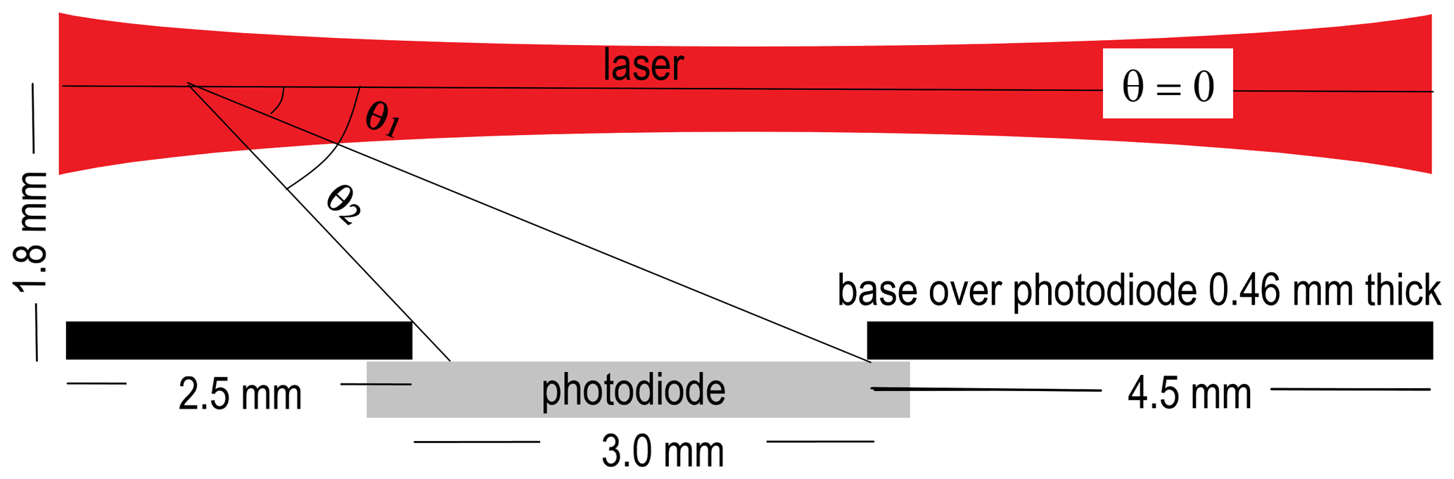
Figure 1PMS sensor geometry highlighting the dimensions of laser beam (red) and photodiode (gray) and the various relevant distances between the two.
Due to the PMS geometry, the upper and lower angular scattering limits for θ depend on the location, x, of a particle in the laser. This can be seen in Fig. S4. For example, at x = 0 mm, at the laser exit, the upper and lower scattering limits for θ are 18–38∘. At x = 4.0 mm, over the center of the photodiode, the angular integration limits are 50–130∘. The PMS photodiode is not capable of detecting light scattered from particles at less than 18∘.
Figures S5–S9 provide more detail about the PMS dimensions and geometry.
2.2.5 PMS5003 sensing volume
The sensing volume is the volume in which the aerosol is irradiated by the laser. The sensing volume extends the length of the laser where the aerosol flows through it, approximately 10 mm. The sensing volume is shown in Fig. S9. The average residence time of a particle in the laser beam is approximately 30 ms. Some of the scattered light is detected by the photodiode and creates a voltage pulse approximately 30 ms wide. It appears that the photodiode is detecting either a cloud of particles from the sensing volume or individual pulses, depending on the concentration. At low concentrations, the aerosol concentration within the sensing volume is unlikely to be uniform, resulting in large relative changes in output per second.
2.2.6 Signal processing and electronics
It is not reported how the PMS MCU differentiates and processes the photodiode signals. The PMS MCU sends the PA-PMS a signal approximately every second in the form of a digital sequence of unsigned 16 bit binary data words, and CH1 is thought to be proportional to the photodiode current. The photodiode current was not measured in this study. The PA creates 80 s (firmware version 3) or 120 s (firmware version 4 and higher) averages and writes them to its micro SD card. We measured an average percentage difference of 0.3 % between the 2 min averages reported by the PA and the 2 min averages calculated from the 1 s values from the PA-PMS. The results are shown in Fig. S10. It is apparent that the processing done by the PA-PMS to calculate its reported 2 min averages does not bias the results.
2.2.7 PA-PMS CH1 variability in sampling filtered air
We found significant variability in PMS response to filtered air. We exposed 21 PA-PMss containing 42 PMS sensors to filtered air for 2 to 94 h. The results are summarized in Table S1. Hourly average CH1 ranged from 0.10 to 377. Overall, 11 PA-PMSs had both CH1A and CH1B averages below 2, while seven PA-PMSs had at least one CH1 average over 26. We recommend that before deployment the PA-PMSs sample filtered air for at least 4 h to identify and eliminate PA-PMSs with CH1 hourly averages over 2 in filtered air. Removing PA-PMSs with high CH1 offsets in filtered air reduces uncertainty and improves precision, particularly in cleaner ambient air.
2.2.8 PA-PMS CH1 unresponsive to CO2 and Suva®
Filtered air, CO2, and Suva® (DuPont™ Suva® 134a refrigerant) are often used to calibrate integrating nephelometers (Anderson et al., 1996). The Rayleigh scattering coefficients of filtered air, CO2, and Suva at 657 nm and at STP (0 ∘C and 1013.25 hPa) are 5.5, 13.3, and 46.2 Mm−1, respectively. We found that the PMS was unresponsive to 100 % CO2 (Fig. S11) and Suva. The CH1 for each gas was the same as filtered air. These results indicate that the PMS signal processing zeroes out a constant scattering signal and cannot be used to measure the scattering coefficient of gases that are commonly used in calibrating nephelometers. Furthermore, the method used by the PMS to subtract light scattering by air molecules in the sampling volume is unknown.
2.2.9 PA-PMS CH1 and CH1avg precision
The PA-PMS CH1 precision was measured by collocating 10 PA-PMS monitors on the roof of the NOAA building in Boulder, Colorado, between 22 January and 1 February 2021. These monitors were not checked with filtered air before deployment. It was found that two of the PMS sensors had large offsets and two had moderate offsets at low CH1 values. One PMS sensor was found to produce errant data and was removed from the analysis, resulting in valid data from 19 CH1A and CH1B sensors in the 10 PA-PMSs.
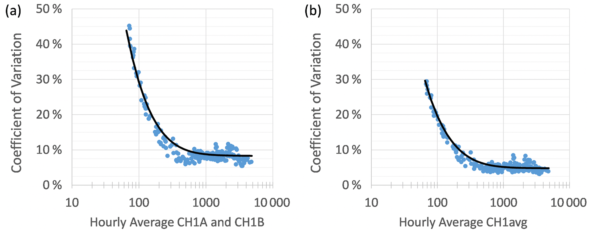
Figure 2Precision estimated as the coefficient of variation of the hourly CH1A and CH1B (a) and CH1avg values (b) for the 19 collocated sensors and 9 PA-PMSs.
The precisions for the hourly data from the CH1A and CH1B sensors and their average (CH1avg) were estimated as the coefficient of variation for each of the 19 CH1A and CH1B values and the 9 CH1avg values for each hour, which are plotted against the average CH1 values in Fig. 2. As shown, above CH1 values of 500, the precision is relatively constant with an average of 8 % and 4.8 % for CH1A–CH1B and CH1avg, respectively. Below CH1 values of 500, the uncertainties increase rapidly with decreasing CH1 values.
There are two mechanisms that may contribute to the rapid uncertainty increase for CH1 < 100. First, it is likely that some of the increased uncertainty in CH1 below values of 100 is inherent to sampling low concentrations, as is the case for any instrument. Second, the geometry of the laser sensing volume in the PMS can contribute to uncertainty in the CH1 at low concentrations, specifically if particles are not distributed uniformly within the laser beam.
The data in Fig. 2 can be modeled by the sum of squares of an additive (Unadd) and multiplicative uncertainty (Unmult) (Currie, 1968; Hyslop and White, 2008, 2009; JCGM100:GUM, 2008):
Equation (1) was fitted to the precision data in Fig. 2 where the Unmult was set to the average precision at high CH1 values, and Unadd was set to 28 and 19 for the A and B sensors and CH1avg, respectively, to fit the highest variances (Table S2). The Unadd is the precision of CH1 as CH1 approaches zero and is assumed to be equivalent to the uncertainty in values below the instrument minimum detection limit (MDL) or that of blanks (Currie, 1968), which were 0.08 and 0.048 for the A and B sensors and CH1avg, respectively. The coefficient of determination in the model fit for both sets of data was r2 = 0.96. Defining the MDL as the 99 % confidence interval of the Unadd (Code of Federal Regulations, 40 CFR 136, https://ecfr.io/Title-40/Part-136, last access: 31 January 2022), MDLs for the individual CH1 sensors and CH1avg were 65 and 44, respectively.
As shown in Sect. S3, the Unmult and Unadd are highly dependent on the systematic biases between the individual CH1 sensors and CH1avg and the four CH1 sensors with data offsets as the CH1 approaches zero (Fig. S12). Removing these four sensors and normalizing the data for each CH1 sensor by their average reduced the Unadd and Unmult to 9 % and 3 %, respectively, for the CH1 sensors and 6 % and 1.9 %, respectively, for the CH1avg data. These results correspond to an MDL of 21 and 14 for the normalized CH1 sensor and CH1avg data, respectively. Based on these results, an “off-the-shelf” PA-PMS will have a CH1avg MDL of about 44 and precision of less than 4.3 %, but the careful selection of a PA-PMS without an offset and that has relatively low noise will have an MDL of 14 and precision of less than 1.9 %.
2.3 Overview of cell-direct and cell-reciprocal nephelometers
The integrating nephelometer was invented during World War II (Beuttell and Brewer, 1949). It provides a direct measure of aerosol light scattering integrated over a large angular range, the “aerosol light scattering coefficient”. This measure requires no assumptions about aerosol composition, size distribution, refractive index, or shape. The most common nephelometer configurations are the “cell-direct” and “cell-reciprocal” ones. Figure 3 presents schematics of the two types of nephelometers. The geometrical relationship between the laser and the photodetector in the PMS resembles a cell-reciprocal nephelometer (Fig. 3b).
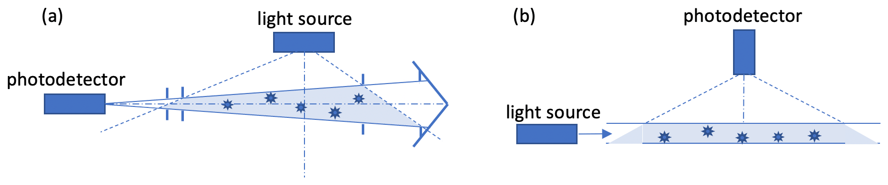
Middleton (1952) was the first to show that the cell-direct nephelometer with a Lambertian (cosine-adjusted diffuser) light source directly measures the aerosol light scattering coefficient. Anderson et al. (1996), following the derivation in Butcher and Charlson (1972), added geometrical diagrams to make Middleton's derivation much clearer. Mulholland and Bryner (1994) proved that the cell-reciprocal nephelometer with a Lambertian diffuser followed by a photodiode placed at the center of the cell-reciprocal nephelometer also directly measures the aerosol scattering coefficient. This put both the cell-direct and cell-reciprocal nephelometers on equal theoretical footing.
There are a number of cell-direct nephelometers in use today. They include the TSI 3563 (St. Paul, MN, USA; Anderson et al., 1996), the Ecotech Aurora models 3000 and 4000 (Knoxfield, Australia; Müller et al., 2011), the Radiance Research M903 (Seattle, WA, USA; Heintzenberg et al., 2006), and the Optec NG-2 (Lowell, MI, USA; Molenar, 1997). In contrast, cell-reciprocal nephelometers have more limited commercial availability. The photoacoustic extinctiometer (PAX; Droplet Measurement Technologies, Inc., Longmont, CO, USA) and the three-wavelength photoacoustic soot spectrometer (PASS-3) use a cell-reciprocal nephelometer to measure the aerosol light scattering coefficient (Arnott et al., 2006). A cosine corrector followed by a photomultiplier tube is placed at the center of the cell-reciprocal nephelometer (Abu-Rahmah et al., 2006; Nakayama et al., 2015).
A “perfect nephelometer” is one in which the nephelometer is able to see the scattered light over the entire angular range from 0 to 180∘. In practice, this cannot be achieved for the cell-direct and cell-reciprocal nephelometers. Both the forward and backward scattering angles are truncated. For example, the TSI 3563 nephelometer has measured angular truncation below about 7∘ in the forward direction and above 170∘ in the backward direction (Anderson et al., 1996; Heintzenberg and Charlson, 1996). For the PASS-3, Nakayama et al. (2015) found that both the large effective truncation angle (21∘) as well as the perpendicular polarization of the 532 nm laser relative to the scattering plane contribute to the large particle size dependence of measured scattering. Light scattering from ammonium sulfate particles of 0.71 µm diameter was reduced by 50 % relative to a perfect nephelometer. Angular truncation generally results in nephelometers underestimating the contribution of particles larger than approximately 1 µm diameter to the scattering coefficient, although corrections have been developed to account for angular non-idealities (e.g., Anderson and Ogren, 1998; Müller et al., 2011).
To gain insight into how the PMS responds to ambient aerosol properties, a model was developed to estimate the intensity of scattered light impinging on the PMS photodiode. The primary purpose of the model was to predict how the PMS performance compares to other instruments designed to measure the aerosol scattering coefficient, such as integrating nephelometers. The model makes simplifying assumptions about the laser that allow the application of Mie theory to the light scattered from particles in the laser. Details of the model are presented in the Appendix.
The equation describing the intensity of light scattered from a particle in the laser is (Middleton, 1952; Anderson et al., 1996)
where I(θ) is the intensity of light at angle θ scattered from a particle in the volume element dv (with units of W sr−1); βp(θ) is the volume scattering function (m−1 sr−1); Fdv is the incident laser flux density (W m−2) impinging on the volume element dv; and dv is the volume element within the laser.
The volume scattering function for a single particle in the laser beam is a function of aerosol diameter Dp, complex refractive index m, laser wavelength λ, and scattering angle θ:
where is the Mie scattering intensity function for laser light polarized parallel to the photodiode surface and perpendicular to the plane of incidence (Bohren and Huffman, 1983).
The scattered light intensity from a single particle in the laser beam to a narrow strip across the middle of the photodiode and from all positions in the scattering volume is integrated to predict the total power received by the photodiode as a function of particle diameter Dp and refractive index m:
Due to the PMS geometry, the upper and lower angular scattering limits for θ depend on the location, x, of a particle in the laser. Details are provided in the Appendix. This approach can be used to estimate the amount of scattered energy detected from mixtures of particles of varying diameters and indices of refraction, as shown in Eq. (5):
3.1 Model predictions – deviation from a perfect cosine response
As discussed above, the PMS has a photodetector that is about 1.8 mm below the laser, resulting in forward scattering and backscattering truncation angles of 18 and 166∘, respectively. Furthermore, the photodetector is recessed 0.46 mm below the scattering chamber base. Equation (4) is used to explore the deviation from a perfect cosine response resulting from the truncated scattering volume and recessed detector. It is shown in Fig. 4. For these calculations, is set equal to 1, which corresponds to isotropic scattering or a volume scattering function that is constant over all scattering angles. It is assumed that the detector has a Lambertian response; i.e., the light detected is independent of the direction of the incident energy, which results in a detector cosine response. Figure 4 shows a perfect cosine response in yellow, while the red line shows the deviation from a perfect cosine response due to angular truncation. The blue line shows the effect of both angular truncation and an inset detector that is 0.46 mm below the chamber base. All curves have been normalized to one at 90∘.
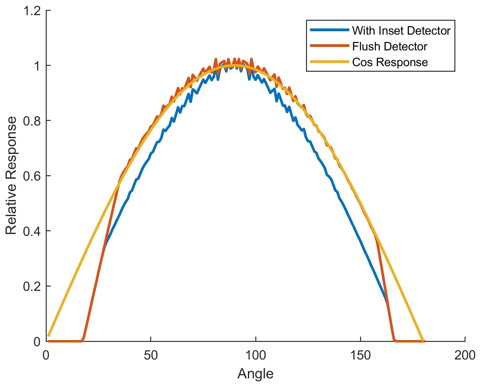
Figure 4Relative response of the photodetector resulting from truncated scattering angles and a recessed photodetector. See the explanation of the different curves in the text.
3.2 Model predictions – intensity versus position on the detector
Figure 5 provides an example of the energy distribution on the photodiode as a function of position in the laser and on the diode resulting from scattering from particles represented by a log-normally distributed aerosol volume size distribution with a volume mean diameter of 0.33 µm and geometric standard deviation of 1.7. Figure 5 shows model predictions of the relative intensity of scattered light, where the values are proportional to energy flux impinging on the detector.
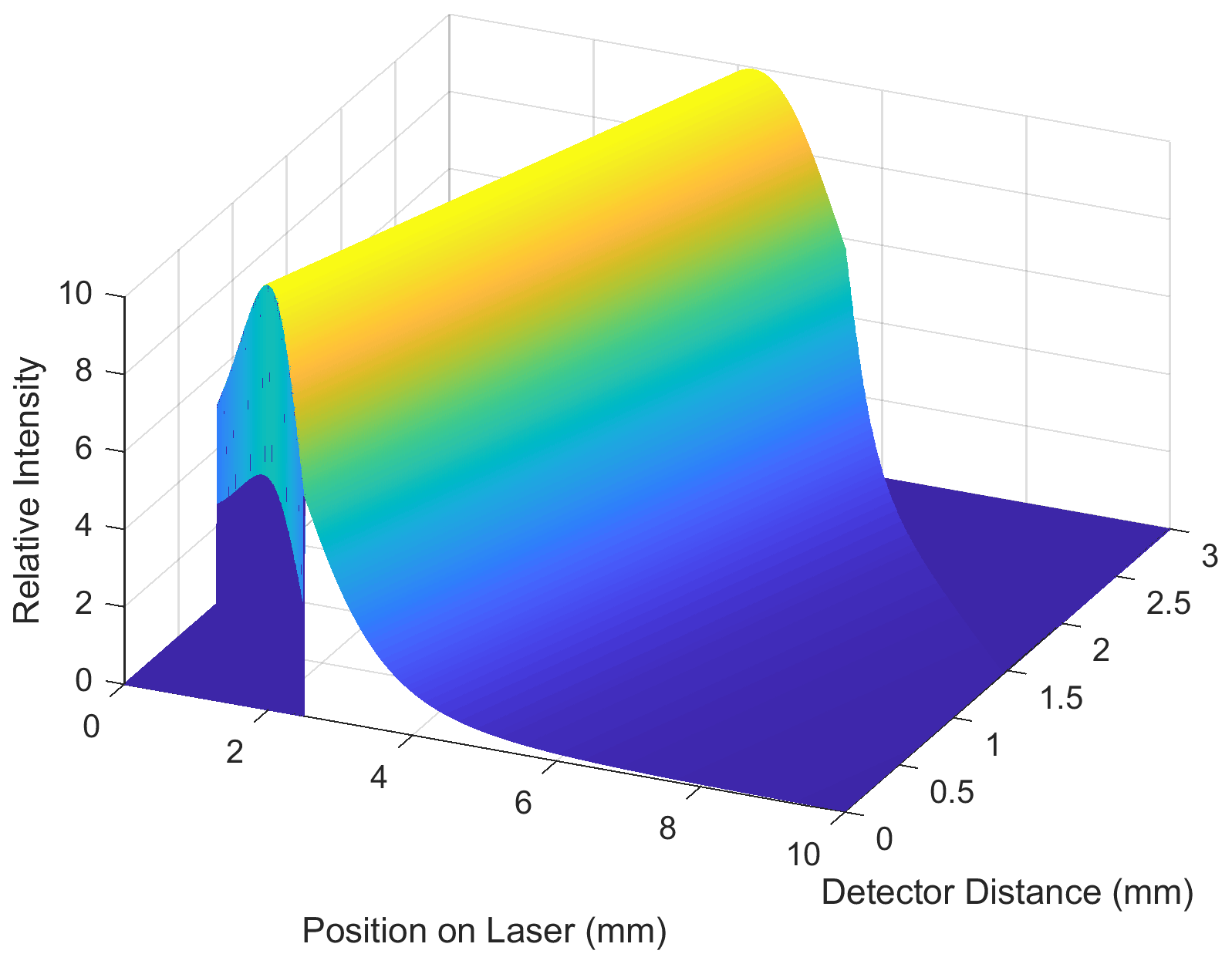
Figure 5Relative intensity of radiant energy scattered by a log-normally distributed aerosol volume size distribution with a volume mean diameter of 0.33 µm and geometric standard deviation of 1.7 as a function of location of scattering event in the laser and as a function of position on the photodiode. Assumed laser wavelength was 650 nm, and the particle index of refraction was assumed to be 1.53. Positions in the laser and detector are from left to right as in Fig. 1 and are in units of millimeters.
The masking resulting from a recessed detector truncates the scattering both in the most forward and most backward scattering angles. This masking is shown as the triangular area corresponding to distance down the laser and detector of 0.0–2.5 and 0.0–0.78 mm, respectively, for the forward scattering angles, and 5.6–10 and 1.44–3.0 mm, respectively, for backscattering. Because the laser is parallel to the photodetector, which is assumed to have a cos (90−θ) response, the maximum energy scattered to the detector is approximately at θ = 90∘. However, more energy is scattered to the detector for scattering angles less than 90∘, which corresponds to forward scattering, and very little energy is detected by the photodiode for particles in the laser that are greater than about 8 mm down the laser beam, even though the detector is exposed to particles in the laser that are 10 mm away from the laser exit hole. These distances down the laser correspond to backscattering. The total energy detected by the photodiode is the sum or integral across both the detector surface and position in the laser and corresponds to the volume under the curve depicted in Fig. 5.
3.3 Model predictions – predicted photodiode response as a function of particle diameter
The PMS differs from a perfect nephelometer in at least five important ways:
-
The laser is polarized, whereas the nephelometer light source is unpolarized.
-
The laser beam profile is not a simple plane wave but complex in shape. The laser beam profile evolves significantly as it is focused over the photodiode.
-
The photodiode likely does not have a perfect cosine response.
-
The PMS geometry limits the photodiode to receiving scattered light between approximately 18 and 166∘, whereas a perfect nephelometer measures all energy scattered between 0 and 180∘.
-
The unknown PMS signal processing removes the light scattering signal from CO2, Suva, and filtered air. These gases are used to calibrate nephelometers but cannot be used to calibrate the PMS.
The effects of these differences can be seen in Fig. 6, which shows predicted photodiode response as a function of particle diameter. The perfect nephelometer response is in blue, and the PMS response is in yellow. The red line predicts PMS response if the laser were not polarized. Relative intensities have been normalized to an ideal nephelometer measurement of a 0.1 µm diameter particle, which is akin to adjusting the laser power such that the scattered power at a diameter equal to 0.1 µm is the same for all configurations. Scattering as a function of particle diameter is nearly the same for all three configurations from 0.1 to about 0.3 µm. At about 0.8 to 1.0 µm, the response of a PMS with an unpolarized laser is about half that of an ideal nephelometer, and the use of a polarized laser reduces its response to about 30 % to that of an ideal nephelometer. For particles above 2 µm in diameter, the PMS response compared to an ideal nephelometer is decreased by about 75 %. Additionally, the PMS manual (Zhou, 2016) quotes a lower detection limit diameter of 0.3 µm. The model predicts that particles smaller than 0.3 µm in diameter would be detected by the PMS, in direct proportion to their contribution to the scattering coefficient.
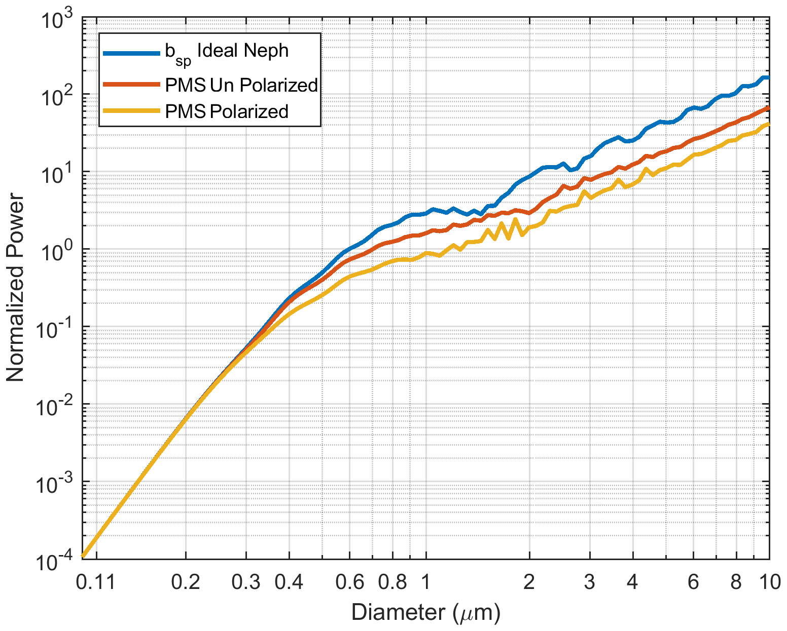
Figure 6Normalized power detected by an ideal integrating nephelometer, a PMS with an unpolarized light source, and a PMS with a perpendicularly polarized light source plotted as a function of particle diameter. Modeled light source wavelength is 657 nm, and the particle index of refraction is 1.53. See the explanation of the different curves in the text.
These differences in geometry and optics from an ideal nephelometer are further highlighted in Fig. 7. To highlight the effect of polarization, the blue line shows the ratio of an ideal nephelometer with a laser light source that is perpendicularly polarized to an ideal nephelometer with an unpolarized light source while the red line shows just the effect of PMS geometry relative to an ideal nephelometer. The yellow line shows the effects that polarization and PMS geometry have on the measured scattering signal. Again, all hypothetical instrument responses have been normalized to a particle diameter of 0.1 µm. Relative to scattering for a 0.1 µm particle, the polarization alone reduces the scattering signal of an ideal nephelometer by 40 % for particles with diameters in the 0.8–1.5 µm size range. The additional effect of PMS scattering geometry reduces the scattering signal at 0.8–1.0 µm by about another 30 % relative to an ideal nephelometer.
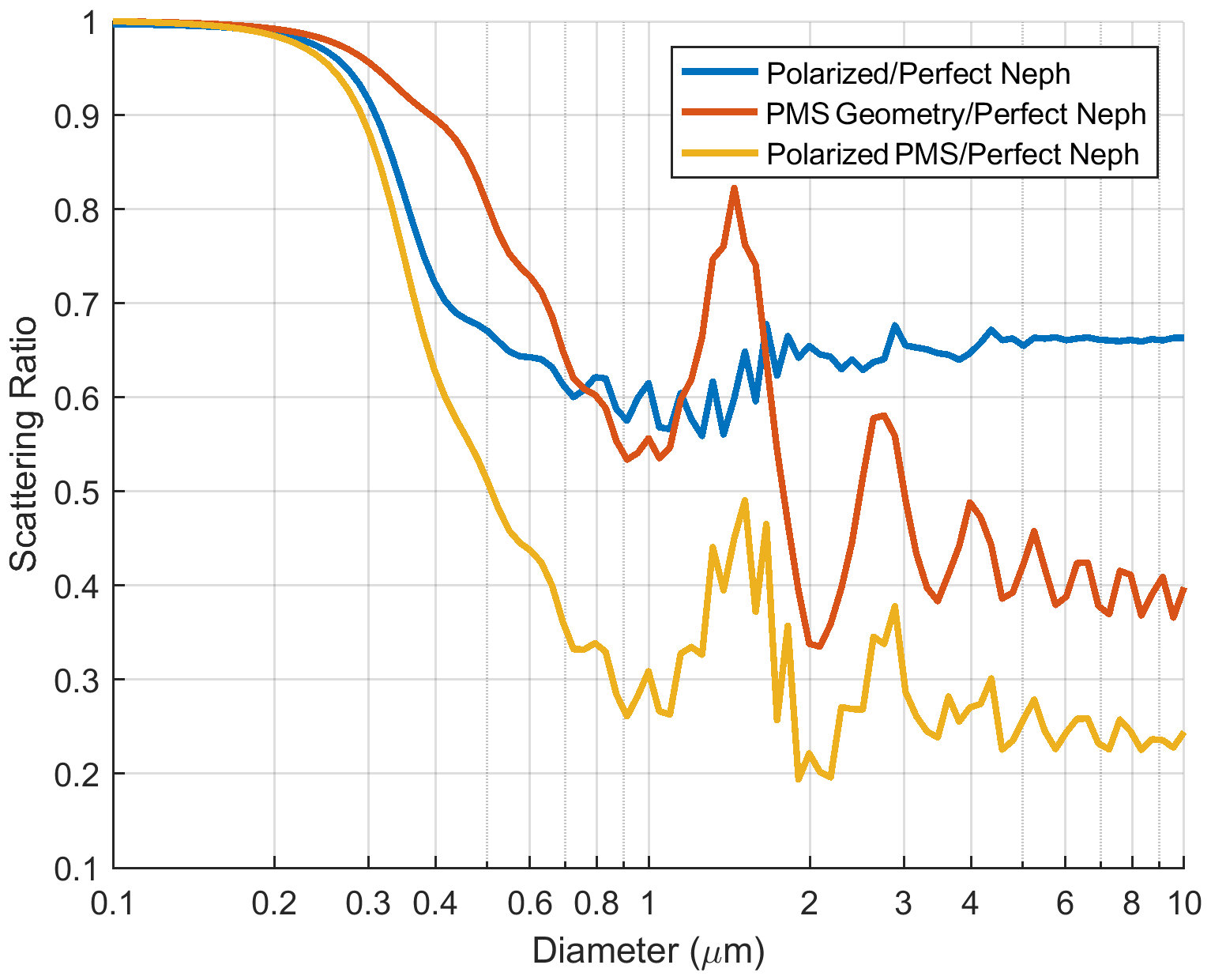
Figure 7Ratio of scattering of a “perfect” nephelometer to a nephelometer with a light source that is perpendicularly polarized (blue) and to a PMS with an unpolarized light source (red). The yellow line shows the effect of a perpendicularly polarized light source and PMS geometry. All three curves are plotted as a function of particle diameter.
As noted in Sect. 2.2.3, the specifications of the BPW34 are used to estimate the likely properties of the detector in the PMS. Our model assumes two ideal properties of the photodiode. The first is area uniformity – that a photon impinging any part of the photodiode would generate the same current as the same photon impinging on another part of the photodiode. The second ideal assumption is that the dependence of the photodiode current on the light intensity is very linear over 4 or more orders of magnitude. If these assumptions do not hold, then the yellow curve in Fig. 7 will change.
The variance in the PMS physical and optical geometry and errors in the measurements are not known but likely small. To evaluate the sensitivity of the modeled PA-PMS scattering to errors in these measurements, the model was exercised with large deviations of ±25 % and ±50 % in these inputs. As shown in Table S3, the errors tend to increase with particle size. The modeled PA-PMS scattering to a perfect nephelometer is most sensitive to errors in the distance from the laser to the photodiode. For particle diameters of 0.5 µm, +25 % and +50 % changes in this distance resulted in maximum differences of 10 % and 20 %, respectively. Based on these results and the fact that the errors in the physical dimensions are less than 25 %, these errors are thought to have a small contribution to the overall modeled PA-PMS scattering error and were not directly accounted for in the analysis. This analysis does not attempt to account for the possibility that the laser beam profile is not a simple plane wave or that the laser beam profile may evolve significantly as it is focused over the photodiode, and the standard plane-wave Mie calculations would no longer apply.
3.4 Model predictions – differentiating by particle size
The irradiance received by the PMS photodiode from a particle of a given diameter and refractive index depends on the particle's location in the laser beam. The model predicts that particles of different sizes may contribute the same irradiance to the photodiode, depending on their location in the beam, or conversely, light scattered by a particle of a given size can vary by more than an order of magnitude.
As an example, the model predicts that all of the particles in Fig. 8 contribute the same irradiance to the PMS photodiode. The smaller particles contribute the same irradiance by scattering in the more effective forward scattering regime. The larger particles contribute the same irradiance by scattering in the less effective backscattering regime. The photodiode and its associated electronics would not be able to differentiate between them. As a result, the model predicts that the values reported in the six PMS particle size channels from > 0.3 to > 10 µm cannot correctly represent the aerosol size distribution.

Figure 8The model predicts that different size particles can generate the same irradiance on the photodiode, depending on their location in the laser beam. In this example, each of the particles would create 1.7 × 10⁻² pW of scattered irradiance on the photodiode.
Field experiments were conducted at two of the NFAN aerosol monitoring stations: the Mauna Loa Baseline Observatory in Hawaii and the Table Mountain Test Facility in Colorado. Both sites have large suites of aerosol instrumentation and daily access for scientists and technicians to inspect, calibrate, and maintain the instruments. These sites also have integrating nephelometers (TSI 3563, St. Paul, MN, USA) against which to evaluate the PA-PMS monitors.
4.1 Description of the Mauna Loa site
The Mauna Loa Baseline Observatory (MLO) is located on the north flank of the Mauna Loa volcano, on the Big Island of Hawaii (19.536∘ N, 155.576∘ W; 3397 m a.s.l.). The observatory is a premier atmospheric research facility that has been continuously monitoring and collecting data on global background conditions and atmospheric change since the 1950s (https://www.esrl.noaa.gov/gmd/obop/mlo/, last access: 31 January 2022). Continuous aerosol measurements at MLO began in the mid-1970s with the installation of condensation particle counters and an integrating nephelometer (Bodhaine and Mendonca, 1974; Bodhaine et al., 1981). MLO lies above the strong marine temperature inversion layer present in the region, which separates the more-polluted lower portions of the island atmosphere in the marine boundary layer from the much cleaner free troposphere. MLO experiences a diurnal wind pattern (Ryan, 1997) that is strongly influenced by the daily heating and nighttime cooling of the dark volcanic lava rock that makes up the mountain. This “radiation wind” brings air up from lower elevations during the daytime, when atmospheric measurements reflect the local mountain environment. In contrast, during the nighttime, downslope winds develop, and the measurements at MLO are typically dominated by clean, free-tropospheric conditions (Chambers et al., 2013). At these times, the aerosol measurements at MLO often reflect some of the cleanest conditions at any station in the Northern Hemisphere. It has long been known, however, that episodic long-range transport of Asian pollution and dust aerosols occurs, most frequently in the springtime (Shaw, 1980; Miller, 1981; Harris and Kahl, 1990), and these aerosol events can influence both the daytime and nighttime measurements at MLO. Consequently, the aerosol levels at MLO vary over a large range, from extremely low to at times mildly elevated. Here, we use observations from the MLO integrating nephelometer to evaluate the PMS sensor.
4.2 Description of the Boulder Table Mountain site
The Table Mountain Test Facility (BOS) is a large restricted-access federal complex located 14 km north of Boulder, Colorado (40.125∘ N, 105.237∘ W; 1689 m a.s.l.). NOAA conducts atmospheric research at this site, and in addition to its NFAN station, it is one of the Global Monitoring Laboratory's seven US Surface Radiation Network (SURFRAD) sites (https://www.esrl.noaa.gov/gmd/grad/surfrad/tablemt.html, last access: 31 January 2022). Many instruments for measuring surface and column aerosol properties are maintained at this location and used for long-term monitoring of the atmosphere.
The BOS site lies just east of the Front Range foothills of the Rocky Mountains and is typical of a semi-arid, high plains environment. It is a high mesa of predominantly grassland with some desert scrub vegetation. The location is well suited for sampling of wildfire smoke plumes during the fire season in the western United States (summer and autumn), dust events at any time of the year, and occasional urban pollution episodes. The NFAN station at BOS (https://www.esrl.noaa.gov/gmd/aero/net/bos.html, last access: 31 January 2022) was completed in September 2019. BOS operates an integrating nephelometer and a differential mobility particle spectrometer (DMPS). Both provided useful data for evaluating some of the predictions from the physical–optical model we developed for the PMS sensor.
4.3 PA-PMS monitors
PA-PMS monitors were installed on the aerosol towers at the MLO and BOS stations, just below the main aerosol inlets. MLO had two PA-PMS monitors, one gently heated and one unheated, whereas BOS had one gently heated PA-PMS monitor. Prior to deployment, the monitors were tested in a filtered air chamber for 4 h to ensure that the 1 h average CH1 values were less than 1 when no particles were present. One of the PMS sensors in the unheated MLO PA-PMS had 1 h average CH1 values of 27 when no particles were present. The heated monitors were wrapped with heating tape and powered by small DC power supplies. All the monitors were covered with stainless-steel flashing 5 cm below the bottom to prevent rain and snow from entering the inlet (Fig. S13).
The PA-PMS monitors were warmed in an effort to reduce the sample RH to be closer to that of the nephelometer, which is unavoidably heated to above-ambient temperatures by the warmth of the laboratory and by the nephelometer's halogen lamp. Because of this warming, the RH inside the nephelometers rarely exceeded 40 %. Both MLO and BOS are low-RH environments under normal conditions, although occasionally moist air masses are encountered. The heating of the monitors increased the sample temperatures by 5–8 ∘C, which helped to lower the sample RH. While the PA-PMS heating was not controlled to achieve an RH match with the nephelometer, it brought the sample RH of the two measurements closer together. The gentle warming of the heated PA-PMS to only a few degrees above ambient is unlikely to cause the PVC to off-gas or melt. Heating from direct sunlight may have had a larger impact.
Due to internet protocols at both sites, the PA-PMS wireless data transmission feature was not used, and the data were stored on the internal micro SD card. At approximately 1-month intervals, the data were downloaded from the micro SD cards, and the PA-PMSs were returned to service. Outputs from the two PMS sensors were then compared at these intervals to determine if the PA-PMSs were still functioning properly. In this study, the 80 s or 2 min averages were used to create 1 h averages to compare the PA-PMS observations to those of the nephelometer and the DMPS.
4.4 Integrating nephelometer
The integrating nephelometer (TSI Inc., model 3563) measures the aerosol light scattering coefficient at three wavelengths (450, 550, and 700 nm). At both sites, the sample flow path is switched every 6 min between 1 and 10 µm aerodynamic diameter, multi-jet, Berner-type impactors. Here, the scattering coefficients at 550 nm for both the PM1 and PM10 size fractions are used for comparison with the PA-PMS measurements. These are referred to as bsp1 and bsp10, respectively.
There are two quality checks of the nephelometer operation made in the field. First, the nephelometer automatically samples filtered air once per hour. This provides a record of the stability of the instrument background measurement. Second, the nephelometer calibration is manually checked on a monthly basis using CO2 and filtered air (Anderson et al., 1996). The 1 h average bsp1 in filtered air is 0.01 Mm−1 with a standard deviation of 0.12 Mm−1, based on 125 h of sampling filtered air.
The nephelometer measurements were corrected for angular truncation (Anderson and Ogren, 1998) and reported at STP. Weekly data review provides quality assurance of the nephelometer data. Scattering coefficient data were averaged to 1 min resolution for logging and were further averaged to hourly resolution for comparison with the PA-PMS data. The 1 h average bsp1 uncertainties of the nephelometer measurements are ∼ 0.13 Mm−1 for scattering coefficients less than 1.0 Mm−1 and ∼ 10 % for scattering coefficients greater than 1 Mm−1 (Sherman et al., 2015).
4.5 Differential mobility particle spectrometer (DMPS)
The DMPS was provided by the Institute for Atmospheric and Earth System Research, University of Helsinki, Finland. It was checked and calibrated by the World Calibration Centre for Aerosol Physics (WCCAP) at Leibniz Institute for Tropospheric Research (IfT), Leipzig, Germany, just prior to deployment at NOAA's Table Mountain site. After shipment from IfT to NOAA, the DMPS was again checked by aerosolizing polystyrene latex spheres and confirming that the peaks occurred in the correct size bins. The DMPS was housed inside the same building as the nephelometer at BOS and sampled aerosols through the same inlet, although the DMPS flow did not pass through the aerosol impactors.
The DMPS provides 40 channels of particle concentration versus size, ranging from mobility diameters of 0.01 to 0.8 µm. The 0.1 to 0.8 µm channels of the DMPS were used to calculate hourly average fine aerosol scattering coefficient distributions and the total fine aerosol scattering coefficient, assuming spherical particles (Mie theory) with a refractive index of 1.53+0.017i. The hourly average, DMPS-calculated fine aerosol scattering coefficients were compared to the nephelometer-measured fine aerosol scattering coefficients to check operational consistency (Fig. S14). No operational changes were made to the DMPS during this field study. This study did not measure coarse aerosol size distributions. The DMPS hourly average fine aerosol scattering coefficient distributions were used with the PMS physical–optical model to predict total 1 h average scattered irradiance on the photodiode.
This section describes our evaluation of the PA-PMS using field data from MLO and BOS. First, we provide an overview of the observational data. We then assess how well the model described in Sect. 3 is able to represent the observed data and show consistency with results previously reported in the literature. Next, we present results showing the potential of the PA-PMS to perform as a nephelometer. Finally, we note how the size information output by the PA-PMS is not correct due to the PA-PMS's primary measurement being a scattering measurement. For the results presented below, data from the PA-PMS, nephelometer, and DMPS were averaged to hourly frequency and merged prior to analysis.
5.1 Field data overview
Heated PA-PMS monitors were deployed at the MLO and BOS observatories for 15 and 11 months, respectively (Table 1). At both sites, weather had no impact on the operation of the PA-PMS instrument, and downtime only occurred during data downloading.
Table 1Summary of PA-PMS, TSI nephelometer, and DMPS data coverage. NA – not available.
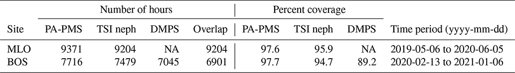
Table 2Summary of PA-PMS and nephelometer hourly observations at MLO and BOS.
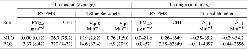
These two deployments provide an excellent dataset for assessing PA-PMS performance in both a clean location (MLO) and in an environment with more elevated particle concentration (BOS). As shown in Table 2, during the field study at MLO, the median CH1 was 26.7. The median bsp1 was 0.76 Mm−1 at 550 nm, which is approximately 10 % of Rayleigh scattering at the MLO altitude. The reported PM2.5 mass concentration from the PA-PMS was zero for most of the MLO deployment. The CH1 and bsp1 are adjusted to STP in Table 2. The air quality at BOS was less pristine than at MLO and is more representative of nonurban continental air quality. The very high maximum CH1 and bsp1 at BOS reported in Table 2 occurred during smoke events in the summer and autumn of 2020. One of the BOS PMS sensors experienced approximately 10 % degradation in sensitivity after 1 year in the field (Fig. S15).
5.2 Relationship between model predictions and field data
The PMS sensor is described by the manufacturer as a particle counter that measures particles between 0.3 and 10 µm in six size bins. Based on the theoretical characterization of the PMS sensor described in Sect. 3, the sensor is more akin to a polarized, reciprocal integrating nephelometer than a particle counter. Below, the field data and theoretical model are used to demonstrate that the raw PMS CH1 sensor signal is an integrated scattering measurement that is sensitive to particles smaller than 0.3 µm but relatively insensitive to particles larger than 1.0 µm.
5.2.1 Predicted photodiode irradiance versus CH1 field data at BOS
Our model, described in Sect. 3 and the Appendix, predicts a value proportional to the scattered irradiance impinging on the PMS photodiode as a function of particle diameter and concentration. This was done using the DMPS size distribution data from BOS. The modeled PMS photodiode output is plotted against the PA-PMS CH1 output (Fig. 9). The predicted photodiode output is linearly correlated with the ordinary least squares (OLS) regression (r2=0.90, normalized root mean square error (NRMSE) ∼ 25 %) with CH1 over 4 orders of magnitude. The RMSE contains contributions of errors from the model-predicted radiant power, the measured scanning mobility particle sizer (SMPS) data the model is based on, as well as in the CH1 measurements. This strong correlation and low RMSE are convincing evidence that the model and SMPS data describe the PMS response quite well.

Figure 9The 1 h average CH1 reported values plotted against model-predicted radiant power (or energy) in µW on the photodiode. Both the CH1 and DMPS data were adjusted to STP conditions. The ordinary least squares regression line is also shown. The plot is based on 6839 1 h averages at BOS.
The linear relationship between CH1 and modeled photodiode response suggests the likelihood that the CH1 output is directly related to what the photodiode is sensing (i.e., scattering from all particles in the scattering volume). The PA-PMS reported values, such as concentrations of particle numbers in various size ranges or PM concentrations, are quantities derived from the scattering signal and the use of an undescribed algorithm.
5.2.2 Predicted aerosol size truncation versus published laboratory data
The PMS physical–optical model described in Sect. 3 predicts that if CH1 is proportional to the photodiode power, then its signal will be reduced relative to a perfect nephelometer. Thus, the ratio of CH1 bsp should decrease as median scattering diameter increases. To test this prediction, data were obtained from published laboratory studies evaluating the PMS against aerosols of varying composition and size distribution reported by Tryner et al. (2019, 2020) and He et al. (2020). These reported aerosol size distributions were used here to calculate the aerosol scattering coefficient distributions from 0.1 to 10 µm for the various aerosols and refractive indices at a wavelength of 657 nm. The median scattering diameter (MSD) was calculated for each test. The MSD is the aerosol diameter at which approximately half of the light scattering coefficient is due to particles smaller than the MSD and the other half to particles larger than the MSD. The MSD was then compared to the ratio of the measured CH1 and bsp10 values, i.e., CH1avg bsp10, for each of the tests reported in Tryner et al. (2020) and He et al. (2020). Figure 10 summarizes the results for CH1 bsp10 versus MSD.
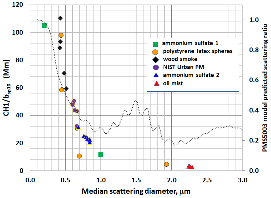
Figure 10Laboratory measurements of CH1 bsp10 versus median scattering diameter from Tryner et al. (2020) and He et al. (2020). Results are compared with PMS physical–optical model prediction of the scattering ratio (yellow line in Fig. 7). The maximum value of 1.0 of the model-predicted scattering ratio is arbitrarily set at a CH1 bsp10 value of 110 Mm. Ammonium sulfate 1 data are from He et al. (2020); all other data are from Tryner et al. (2019, 2020).
The controlled laboratory results are in general agreement with the PMS physical–optical model, showing substantial reduction in CH1avg bsp10 as a function of increasing particle diameter from 0.2 to 1 µm. The laboratory results show an even greater reduction in CH1avg bsp10 than the model predicts at diameters larger than 1 µm. This suggests the possibility of supermicron aerosol loss before laser detection, perhaps due to aspiration, as discussed in Sect. 2.2.1.
5.2.3 CH1avg bsp1 as a function of median scattering diameter
Although ambient aerosols may vary considerably in composition and morphology and cannot be as simply characterized as laboratory aerosols, it is instructive to evaluate if PMS angular truncation can be observed using field data. The DMPS data from BOS were used to calculate hourly average aerosol scattering coefficient distributions for diameters between 0.1 and 0.8 µm. A wavelength of 657 nm and a particle refractive index of 1.53+0.0i were used for the calculations. The median scattering diameter was calculated for each hour. The MSD was then compared to the ratio of the measured CH1 and bsp1 values, i.e., CH1avg bsp1, for each of these hours. The results are shown in Fig. 11 as a box-and-whisker plot of the CH1avg bsp1 values found in each MSD bin. The center MSD value for each bin is based on a logarithmic scale of MSD values where the upper and lower bin values are selected as MSDi + MSD and MSDi − MSD and i refers to the ith bin. The thin black horizontal lines correspond to the number of observations in each bin and the scale is shown on the right-hand axis. There are less than 20 values in the 0.22, 0.63, 0.71, and 0.79 µm bins. Approximately 67 % of the MSDs observed at BOS were between 0.29 and 0.36 µm, and 98 % of MSDs were between 0.26 and 0.46 µm. The overall average CH1avg bsp1 ratio, based on 6777 observations, is 65 Mm.
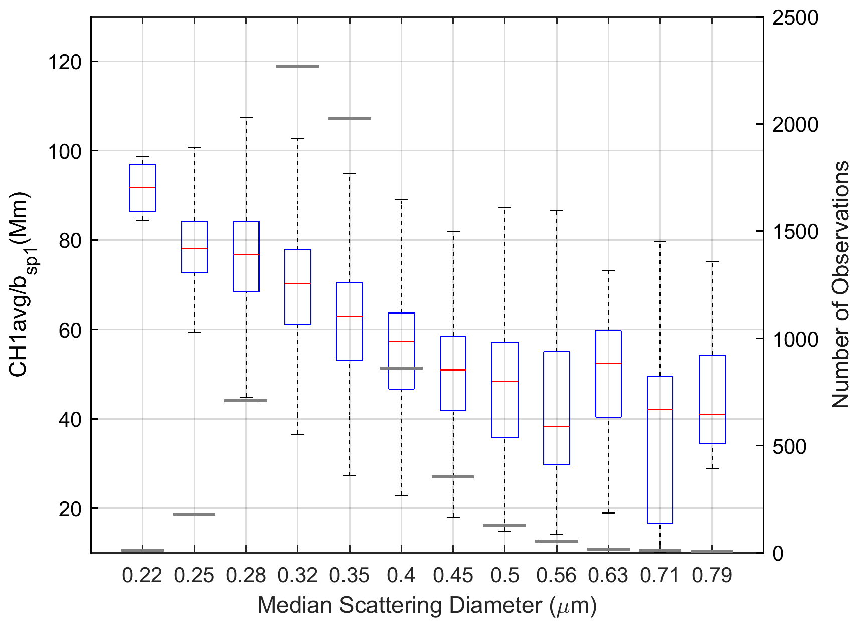
Figure 11Observed decrease in CH1avg bsp1 ratio as a function of MSD values. MSD values were selected based on a log scale but plotted equally spaced from each other to maintain uniformity in the dimensions of the box-and-whisker symbol. The red line represents the median value, and the bottom and top of each box are the first and third quartile values. Extremes shown on each box are the 2nd and 98th percentiles. Black horizontal lines for each MSD value are the number of observations in the respective MSD bins.
Figure 11 is consistent with the PMS physical–optical model. The highest CH1avg bsp1 ratios tend to occur for aerosols with the lowest MSD and decrease as MSD increases. Additionally, the results show, as suggested above, that the PMS can detect particles below 0.3 µm in diameter in proportion to their contribution to the scattering coefficient.
5.2.4 Estimating the scattering coefficient minimum detection limit of the PA-PMS
The precision analysis in Sect. 2 indicates that the PA-PMS monitors used in this study estimated 1 h average CH1 and CH1avg MDLs of approximately 21 and 14, respectively. The estimated 1 h average MDL bsp1 of the TSI 3563 nephelometer is approximately 0.20 Mm−1, based on filtered air tests. Further analysis of the relationship between CH1 and bsp1 at low levels was performed by plotting the ratio, CH1avg bsp1, for the combined MLO and BOS dataset, as a function of bsp1. This relationship is shown graphically in Fig. 12. The data values were first averaged over 6 h because hourly bsp1 values near zero included many small negative bsp1 values due to the very clean conditions occasionally observed at MLO. The averaging eliminated all but five negative bsp1 values, which were removed from the dataset. The CH1avg bsp1 and bsp1 values were further averaged over six data points after sorting the data on bsp1 levels to more clearly show the relationship between CH1avg and bsp1. At bsp1 > 5 Mm−1, the CH1avg bsp1 ratio is relatively constant at 67 Mm (the yellow line in Fig. 12). The yellow line is the slope of CH1avg versus bsp1 at bsp1 values greater than 5 Mm−1. The CH1avg bsp1 ratio systematically decreases from its highest values to about 35 Mm, the slope of CH1avg versus bsp1 at bsp1 = 0.4 Mm−1. For bsp1 < 0.4 Mm−1, the CH1avg bsp1 ratio then increases significantly as bsp1 decreases, consistent with CH1avg values staying approximately constant below 0.4 Mm−1. Both the CH1avg and bsp1 are below MDL for bsp1 < 0.2 Mm−1. A CH1avg bsp1 ratio of approximately 35 Mm at bsp1 = 0.4 Mm−1 and a CH1avg value of about 14 ± 5 is consistent with the estimated CH1avg MDL of 14.
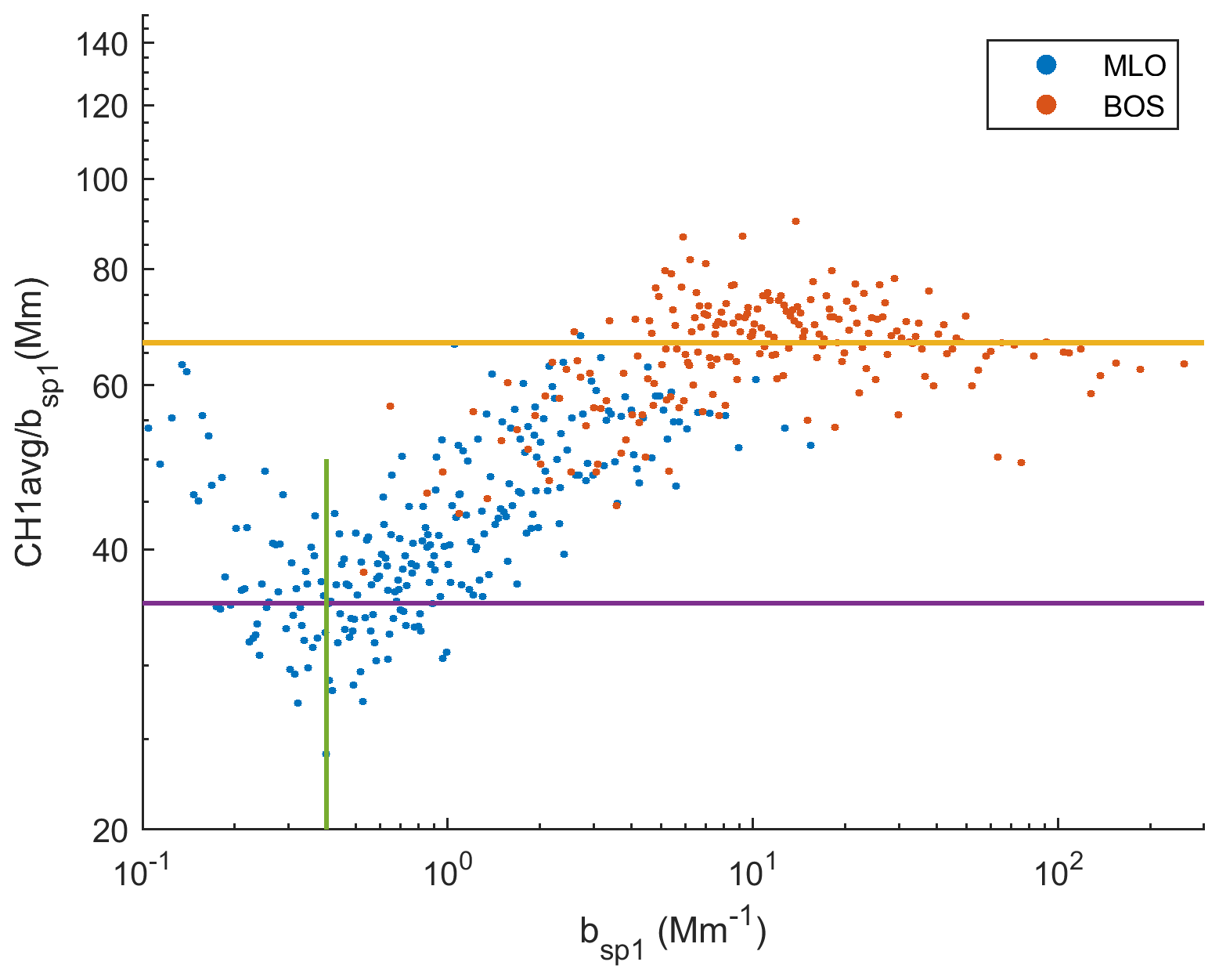
Figure 12Ratios of CH1avg and measured scattering, bsp1, as a function of measured bsp1 for MLO and BOS. The green line corresponds to 0.4 Mm−1, while the purple line, a ratio of 35 Mm, corresponds to the additive uncertainty of 14. The yellow line corresponds to a CH1avg bsp1 ratio of approximately 67 Mm, the slope of CH1avg vs. bsp1 above about 5 Mm−1.
Based on these results, the 1 h average CH1 sensor MDL for hourly data in units of scattering is approximately 0.4 Mm−1 at MLO. Laboratory tests challenging the PA-PMSs with known low-level, spiked aerosol concentrations and defined size distributions are needed to further refine the estimated MDL.
5.2.5 Evaluating the use of the PA-PMS as an integrating nephelometer
The MLO and BOS hourly average CH1avg are plotted against bsp1, measured at 550 nm, in Fig. 13. Also shown in Fig. 13 is an OLS regression line with the intercept set equal to zero using the BOS and MLO combined dataset but with values associated with bsp1 less than 0.4 Mm−1 and greater than 500 Mm−1 removed. Results of the regression for the combined datasets as well as for the individual BOS and MLO datasets are presented in Table 3. There is good agreement for both datasets (Table 3) with an r2 of 0.97 and 0.85 for the BOS and MLO datasets, respectively, and 0.97 for the combined datasets. The relationship deviates somewhat from linear with increasing slopes and scatter at lower values of atmospheric scattering coefficient, particularly for the MLO data. The slopes (in Mm−1) for all data, MLO, and BOS, are 0.015 ± 2.07 × 10⁻⁵, 0.017 ± 5.72 × 10⁻⁵, and 0.015 ± 2.68 × 10⁻⁵, respectively. In the following analysis, a PA-PMS-derived atmospheric scattering (bsp1,PA, Mm−1) for both MLO and BOS is estimated using bsp1,CH1 = 0.015 × CH1avg at a wavelength of 550 nm. The best-fit value of 0.015 Mm−1 corresponds to the yellow horizontal line in Fig. 12 of 67.0 () and corresponds to a median scattering diameter of about 0.33 µm (Fig. 11).
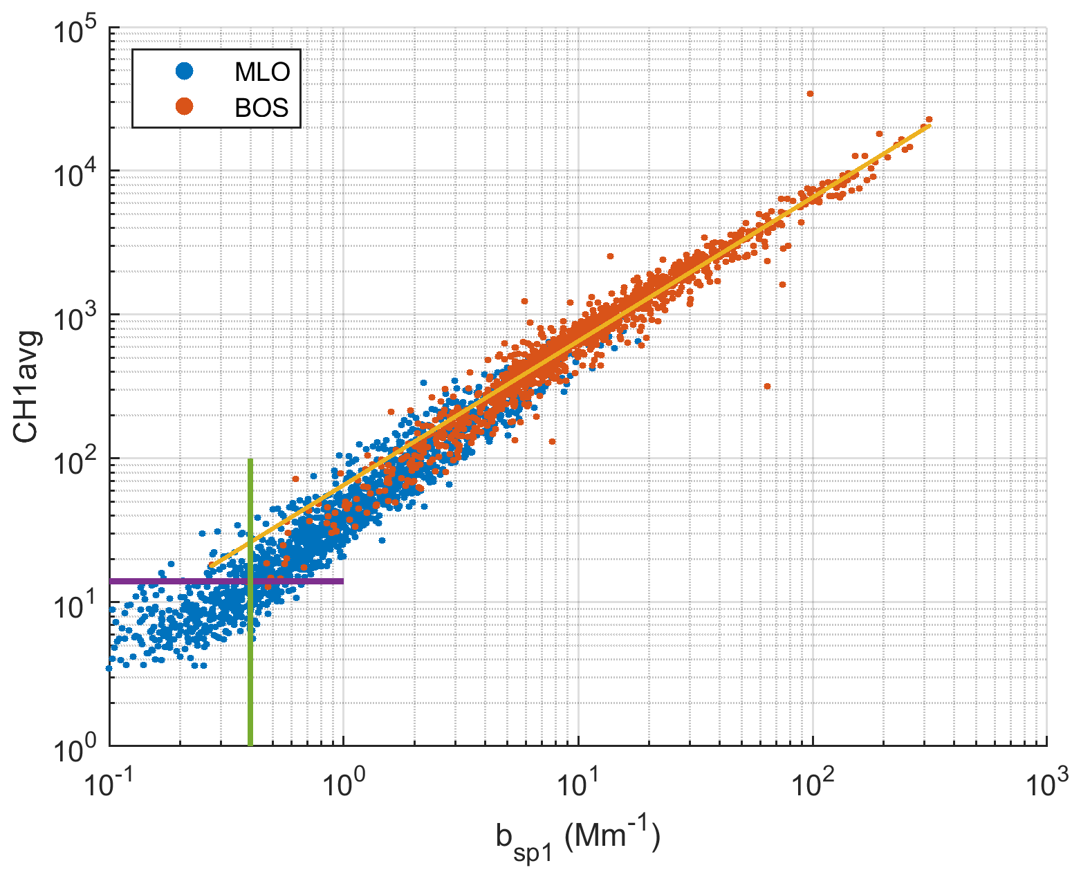
Figure 13Fine aerosol scattering coefficient from TSI nephelometer vs. CH1avg value from PA-PMS. Yellow line represents the fit to all data. The purple line shows the additive uncertainty of 14, while bsp1 values lower than the green line were removed for the regression analysis.
Table 3Ordinary least squares regression coefficients with a zero intercept and standard error for bsp1 and CH1 as the dependent and independent variables, respectively, for the BOS, MLO, and combined datasets. CH1 and bsp1 reported at STP. Also shown are the respective coefficients of determination, r2.
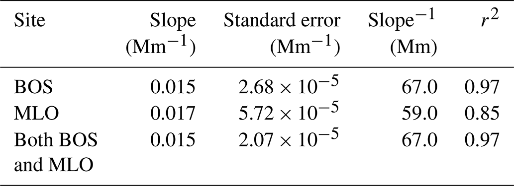
Figure S16 shows that the submicron aerosol scattering coefficients at 550 and 700 nm are highly correlated, with the 700 nm scattering coefficient averaging 52 % of the 550 nm scattering coefficient. This results in bsp1,CH1 = 0.0078 × CH1avg at a wavelength of 700 nm.
As discussed above, the regression coefficient between bsp1 and CH1 for the combined dataset of 0.015 Mm−1 is used to estimate the bsp1,PA derived from the CH1 channel. The data for each dataset and the combined dataset were binned into 10 bins based on measured bsp1 levels that ranged from 0.4 to 500 Mm−1. Values of bsp1 above 500 Mm−1 were removed from the dataset. For each bin, the NRMSE between bsp1,PA and measured bsp1 was calculated. The NRMSE values as a function of the bsp1 bins are plotted in Fig. 14 for the combined dataset represented as the gray bars and BOS and MLO represented by blue and orange bars, respectively.
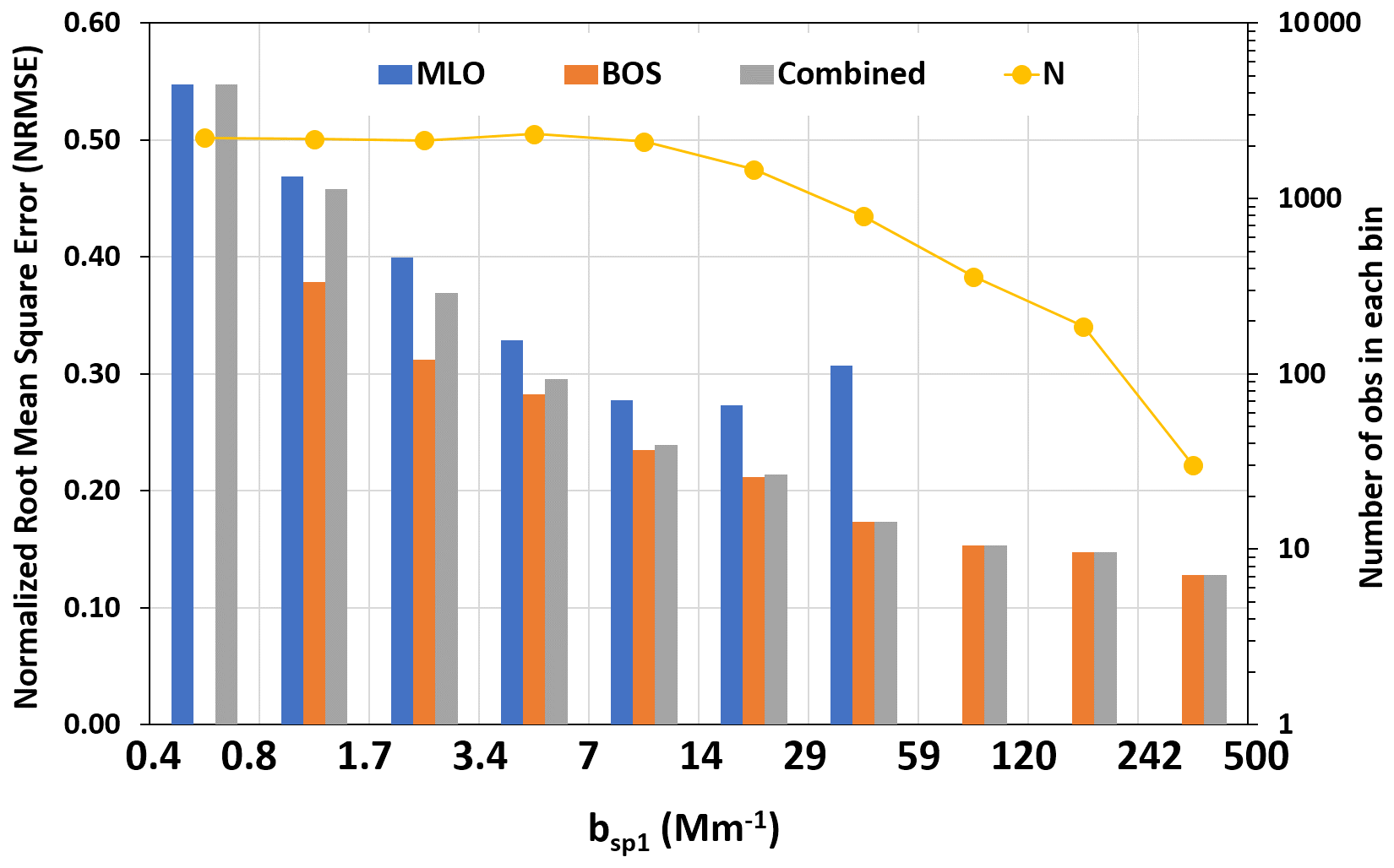
Figure 14Normalized root mean square error between measured and estimated scattering from CH1 values plotted as a function of binned bsp1 for the BOS, MLO, and combined datasets. The yellow line is referenced to the right axis to provide the number of observations in each bin. Numbers on the x axis represent the lower and upper levels of each scattering bin.
For bsp1 levels less than 0.8 Mm−1, the NRMSE is 45 %–55 %, and for bsp1 levels greater than 10 Mm−1, the NRMSE is about 25 % or less. For bsp1 levels greater than 60 Mm−1, the NRMSE approaches 15 %.
As discussed in Sect. 2.2.9, the uncertainty for high CH1avg values is small (1.9 % to 4.8 %). The precision of the TSI 3563 nephelometer is also similarly high, and together they account for about 10 % NRMSE at high bsp1 values.
The overall normalized error is likely due to a variety of sources, primarily the variability in the CH1 values due to using a polarized light source and truncation errors due to the geometry of the PA-PMS sensors. Also, the variability in aerosol characteristics such as size distribution, refractive index, and shape may be important. At extremely low levels, uncertainty may also be due to a nonuniform distribution of particles in the PMS laser beam.
There are two reasons why the PA-PMS MDL and RMSE values reported in our study are surprisingly low. The TSI 3563 nephelometer has an extremely low detection limit of 0.20 Mm−1, which is approximately 1 % of Rayleigh scattering. Second, the PA-PMS has very low noise at zero aerosol concentration. If the PA-PMS in our study had been collocated with a nephelometer that was not as sensitive as the TSI 3563 in a location having an average fine aerosol coefficient of, say, 30 Mm−1, then the PA-PMS 1 h average MDL could have been significantly higher than the 0.4 Mm−1 we obtained in our study.
5.2.6 PA-PMS size distributions
The aerosol number concentrations from the six PMS size channels are unrealistic. The BOS field data showed that the concentration of particles larger than 0.3 µm diameter calculated from the DMPS averaged 10 times higher than CH1 (Fig. S17). The other PMS size channels are so highly correlated with CH1 that they provide no additional information (Table S4). Furthermore, it appears that the PMS creates an approximately invariant normalized aerosol number distribution across a wide range of sites (Table S5, Fig. S18). Although the overall CH1 concentration can vary over 6 orders of magnitude (column 3 in Table S5), the shape of the PMS size distribution remains fairly constant.
In our study, we found that the ambient aerosol size distributions measured with the SMPS varied considerably at Table Mountain, as seen in Fig. 11, while the PA-PMS normalized reported size distribution changed very little. Invariant PA-PMS size distributions were also observed during controlled laboratory studies (He et al., 2020; Kuula et al., 2020; Tryner et al., 2020). This suggests that the values in the channels above CH1 are software generated and indicates that the most relevant output from the PMS is from the CH1 channel. The bottom row of Table S5 shows that the PMS bin fractions above 1 µm increased by only a factor of 2–5 in a high-PM2.5 windblown dust episode at Keeler, California. This is consistent with the PMS model prediction that PMS coarse aerosol response is small relative to a perfect nephelometer.
The results above indicate that CH1 is the primary source of aerosol information from the PMS sensor. Additionally, consistent with the sensor behaving like a cell-reciprocal nephelometer, it was found that CH1 was proportional to the aerosol scattering coefficient, not the number concentration of particles having diameters greater than 0.3 µm. CH1 was approximately a factor of 10 lower than the DMPS number concentration for a similar size range.
5.2.7 Relationship between CH1 and PM2.5
The PM2.5 mass concentration was not measured by Federal Reference Method (FRM) or Federal Equivalent Method (FEM) instruments at MLO and BOS during this study. Consequently, the PA-PMS PM2.5 or CH1 results cannot be compared with PM2.5 concentrations, but they can be compared with measured scattering coefficients and discussed in the context of mass scattering efficiency, which ties scattering coefficient to mass concentration.
Figure S19 shows that the PA-PMS PM2.5 channel is reasonably well correlated with bsp1 for values greater than about 10–20 µg m−3, typical of many moderately polluted locations, with a calculated mass scattering efficiency of approximately 2.5 m2 g−1. This value of the mass scattering efficiency is at the low end of the range of values reported by Hand and Malm (2007), which could reflect the nature of the observed aerosols or an error of the PA-PMS PM2.5 mass concentration. This suggests that the effectiveness of the PA-PMS to serve as a PM2.5 mass concentration monitor is due both to the sensor behaving like an imperfect integrating nephelometer and to the mass scattering efficiency of ambient PM2.5 aerosols being roughly constant with values in the 2–4 m2 g−1 range. However, it is likely that the PA-PMS underestimates PM2.5 for very clean areas where bsp1 is often less than 10 Mm−1. For example, the PA-PMS PM2.5 was zero for 1099 of the hours in this study when bsp1 was greater than 1 Mm−1.
One may obtain a lower bound estimate of the PA-PMS RMSE 1 h average mass concentration from the study results. Figure 14 shows the PA-PMS scattering coefficient RMSE as a function of the measured scattering coefficient. For example, the PA-PMS NRMSE is 20 % for a fine aerosol scattering coefficient of 25 Mm−1. For an aerosol having a mass scattering efficiency of 2–3 m2 g−1, this is approximately 10 µg m−3. Thus, the PA-PMS 1 h average RMSE is roughly 2 µg m−3. This is somewhat lower than the reported mean absolute error of ∼ 4 µg m−3 for hourly average PM2.5 in Pittsburgh (Malings et al., 2020). This error assumes that the mass scattering efficiency is fixed and known. This is generally not the case, and the actual error in the mass concentrations will be larger.
The mean 1 h average fine aerosol scattering coefficient bsp1 at MLO during our yearlong study was 1.50 Mm−1. From Fig. 14, PA-PMS had a RMSE of 0.60 Mm−1. For an aerosol having a mass scattering efficiency of 2–3 m2 g−1, this corresponds to a 1 h average RMSE of roughly 0.2–0.3 µg m−3. This is well below the advertised 1 h average MDL of commercial PM2.5 monitors. For example, the BAM 1020 specifies a typical hourly detection limit of 3.6 µg m−3.
We have demonstrated that the PMS sensor inside the PA monitor (PA-PMS) appears to behave as an imperfect reciprocal integrating nephelometer. As a scattering sensor, the PMS cannot directly count nor size particles in the air stream. The PMS uses an unknown algorithm to convert the scattering signal to a near-constant normalized number distribution from which PM concentrations are derived.
The scattering coefficient that is measured by an ideal integrating nephelometer does not need correction for any aerosol attributes such as shape, chemical composition, refractive index, or diameter. It is a valuable measure for visibility and global climate monitoring. Simple low-cost sensors such as the PA-PMS can play a role in estimating aerosol scattering coefficients and improving global coverage. Yearlong field data at NOAA's Mauna Loa Observatory and Boulder Table Mountain sites show that the 1 h average of the PA-PMS CH1 is highly correlated with a nephelometer-measured fine aerosol scattering coefficient at 550 nm, bsp1, over a wide scattering coefficient range of 0.4 to 500 Mm−1. The relationship between CH1 and bsp1 at 550 nm is found to be bsp1 (Mm−1) = 0.015 × CH1 when both quantities are adjusted to the same temperature and pressure.
The physical–optical model developed in this paper for the PMS and the general consistency with both published laboratory data for a variety of fine aerosols and ambient field data may motivate users of other low-cost sensors to develop similar models. It is possible that some of the other low-cost sensors also use polarized lasers in a cell-reciprocal configuration like the PMS. Such models would improve the understanding of sensor operation and help users better recognize the opportunities and limitations of other low-cost sensors in applications such as monitoring the scattering coefficient.
The strong relationship between bsp1 and CH1 and the general agreement between the model and published laboratory data support characterizing the PMS as an imperfect truncated cell-reciprocal nephelometer. The results demonstrate that it is possible to use the PMS to estimate the 1 h average fine aerosol scattering coefficient across a wide range of aerosol scattering concentrations, provided the aerosol median scattering diameter is between 0.26 and 0.46 µm. The CH1 and bsp1 relationship is dependent on the size distribution, and it is expected to change for locations and times where the particle size shifts to larger or smaller sizes than those measured at BOS and MLO.
We found that the PMS has important limitations compared to integrating nephelometers. It measures the light scattering over a smaller angular range, causing a significant truncation of the scattering signal in the forward and backward directions. Additionally, the PMS uses a polarized light source; the sensor most likely does not have a cosine response; the laser beam profile is not a simple plane wave; and the inlet and sensor geometry creates a broad uncertain particle size cut point. Nephelometers calibrate their scattering coefficient with CO2 or Suva, but the PMS is unresponsive to these gases. As a result, there is currently no convenient way to calibrate the PMS to ensure its accuracy. Neither PurpleAir, LLC nor Plantower provide technical support. Quality assurance and control are not as robust as one encounters for regulatory and scientific monitoring instruments. For this reason, it is useful to test the PMS sensors in filtered air before using them and to limit field use to those sensors that have 1 h average CH1 values less than 2. While sampling, it is necessary to compare 1 h averages from the two PMS sensors in each PA-PMS monitor to become aware of any changes and, if needed, to replace them in a timely fashion.
This study limited its findings to low-RH air, because both the PA-PMS monitors and the nephelometers were heated to reduce RH. Since RH plays such an important role in water uptake by hygroscopic aerosols and the concomitant increase in the scattering coefficient, future work is planned to compare unheated PA-PMS monitors with an unheated nephelometer that does not reduce RH before sampling. Our model predicts that the PMS may not be as responsive to hygroscopic growth as an unheated nephelometer. This is a topic of current study.
The PA-PMS reports a mass concentration of PM2.5 particles, and many papers have been written to compare the PA-PMS values with reference instruments and explain the observed differences. The modest agreement that has been reported is the direct result of two factors generally overlooked in those publications: the PA-PMS behaves like an imperfect integrating nephelometer that provides a representative value of the light scattering coefficient, and the mass scattering efficiency of PM2.5 aerosols is roughly constant, with values in the 2–4 m2 g−1 range.
The PMS physical–optical model makes some simplifying assumptions. The actual PMS laser beam profile is not a simple plane wave but complex in shape. The model assumes the laser is a plane wave with a constant laser beam irradiance profile. This allows the use of Mie theory to predict the light scattered by particles in the laser. Secondly, the model calculates the light scattered to a narrow strip across the middle instead of the entire photodiode. It assumes that the irradiance received by the narrow strip is representative of the entire photodiode.
The intensity of light scattered from a particle in the laser is
where I(θ) is the intensity of light at angle θ scattered from a particle in the volume element dv (with units of W sr−1); β(θ) is the volume scattering function (m−1 sr−1); Fdv is the incident laser flux density (W m−2) impinging on the volume element dv; and dv is the volume element within the laser.
The volume scattering function for a monodisperse aerosol having a diameter Dp and number concentration N(Dp) in the PMS laser is
where is the perpendicular scattering intensity function; λ is the laser wavelength; m is the particle complex refractive index; θ is the scattering angle; and Dp is the aerosol diameter. Note that θ = 0 in the direction of the laser, and θ = 90∘ perpendicular to the laser and photodiode.
For one particle of size Dp in the volume element dv, N(Dp) .
The incremental power dP (watt) scattered from a particle in the volume element dv across a solid angle dΩ subtended on the surface of a sphere at distance r from the particle, and normal to r, is
dΩ = dA0 r2, where dA0 is the incremental area on the sphere at distance r from the particle and normal to r. dP is then
For the PMS model, dA0 is a small rectangle with width w and height rdθ, where w is the width of the strip on the photodiode, and dθ is the differential scattering angle.
dA0 = rdθ × w, where w is the width of the strip on the photodiode. From Fig. A1, , where b is the distance from the laser to the photodiode.
The incremental power across the solid angle dΩ normal to r is then
Substituting for I(θ),
Equation (A7) can be further simplified by combining the constants into , where K has units of watts:
The power received by the photodiode from a particle of diameter Dp in the volume element at x is obtained by numerically integrating across θ on the photodiode:
Due to the PMS geometry, the upper and lower angular scattering integration limits for θ depend on the location x. This can be seen in Fig. S4. For example, at x = 0 mm, the upper and lower integration limits for θ are 18 to 38∘. At x = 4.0 mm, over the center of the photodiode, the angular integration limits are 50 to 130∘.
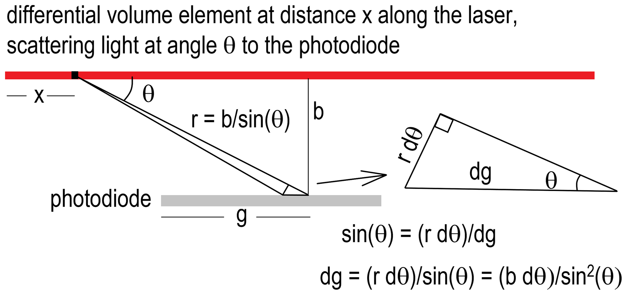
The total power P in Watts received by the photodiode from the light scattered by all the particles of diameter Dp in the laser is obtained by carrying out the numerical integration in Eq. (A9) for all x from 0 to 10 mm:
The result for carrying out this calculation for the power per particle of size Dp is in Table S6 for wavelength 657 nm and particle refractive index 1.53+0.015i. The total power received at the photodiode by a distribution of particles is obtained by summing up the power per particle of size Dp times the number of particles N(Dp,m) in the size interval Dp to Dp+dDp.
Figure A1 shows the PMS geometry. The distance along the laser is the variable x, which ranges from 0 to 10 mm. The distance along the photodiode is the variable g, which ranges from 0 to 3.0 mm. The distance between the photodiode and the laser is b, approximately 1.8 mm.
Datasets are available at http://zenodo.org (last access: 31 January 2022). The dataset is available at https://doi.org/10.5281/zenodo.5764982 (Ouimette et al., 2021). The data were published on 15 December 2021. In our analysis, we also made use of a dataset published by Tryner et al. (2019, https://doi.org/10.25675/10217/195445).
The supplement related to this article is available online at: https://doi.org/10.5194/amt-15-655-2022-supplement.
PJS and JRO designed the field study. PJS provided measurement data from the MLO and BOS sites. BAS performed the uncertainty and precision analyses. WCM led the physical–optical model development with BAS and JRO. JRO and WCM performed analysis of laboratory and field data for model evaluation. WPA provided insight regarding the laser behavior and instrument electronics. JAO and WCM independently performed the statistical analyses of the TSI nephelometer and PA-PMS data. JAO and JRO performed measurements and tests to characterize the PMS5003. EA led the manuscript submission and review process. All authors read and commented on the article.
The contact author has declared that neither they nor their co-authors have any competing interests.
The assumptions, findings, conclusions, judgments, and views presented herein are those of the authors and should not be interpreted as necessarily representing NOAA or National Park Service policies. Reference to any companies or specific commercial products does not constitute endorsement by NOAA or the National Park Service.
Publisher’s note: Copernicus Publications remains neutral with regard to jurisdictional claims in published maps and institutional affiliations.
The authors acknowledge the following for their contributions: Jim Wendell, NOAA, for engineering support, Marty Martinsen, NOAA, for MLO field support, Derek Hageman, CIRES, University of Colorado, for data acquisition and processing support, and Helene Bennett, CIRA, Colorado State University, for technical editing support.
This research has been supported by the National Park Service (grant no. P17AC00971).
This paper was edited by Darin Toohey and reviewed by R. Subramanian and one anonymous referee.
Abu-Rahmah, A., Arnott, W. P., and Moosmuller, H.: Integrating nephelometer with a low truncation angle and an extended calibration scheme, Meas. Sci. Technol. 17, 1723–1732, https://doi.org/10.1088/0957-0233/17/7/010, 2006.
Anderson, T. L. and Ogren, J. A.: Determining aerosol radiative properties using the TSI 3563 integrating nephelometer, Aerosol Sci. Technol., 29, 57–69, https://doi.org/10.1080/02786829808965551, 1998.
Anderson, T. L., Covert, D. S., Marshall, S. F., Laucks, M. L., Charlson, R. J., Waggoner, A. P., Ogren, J. A., Caldow, R., Holm, R. L., Quant, F. R., Sem, G. J., Wiedensohler, A., Ahlquist, N. A., and Bates, T. S.: Performance characteristics of a high-sensitivity, three-wavelength, total scatter/backscatter nephelometer, J. Atmos. Ocean. Technol., 13, 967–986, https://doi.org/10.1175/1520-0426(1996)013<0967:Pcoahs>2.0.Co;2, 1996.
Andrews, E., Sheridan, P. J., Ogren, J. A., Hageman, D., Jefferson, A., Wendell, J., Alastuey, A., Alados-Arboledas, L., Bergin, M., Ealo, M., Hallar, A. G., Hoffer, A., Kalapov, I., Keywood, M., Kim, J., Kim, S. W., Kolonjari, F., Labuschagne, C., Lin, N. H., Macdonald, A., Mayol-Bracero, O. L., McCubbin, I. B., Pandolfi, M., Reisen, F., Sharma, S., Sherman, J. P., Sorribas, M., and Sun, J. Y.: Overview of the NOAA/ESRL Federated Aerosol Network, Bull. Am. Meteorol. Soc., 100, 123–135, https://doi.org/10.1175/bams-d-17-0175.1, 2019.
Arnott, W. P., Walker, J. W., Moosmuller, H., Elleman, R. A., Jonsson, H. H., Buzorius, G., Conant, W. C., Flagan, R. C., and Seinfeld, J. H.: Photoacoustic insight for aerosol light absorption aloft from meteorological aircraft and comparison with particle soot absorption photometer measurements: DOE Southern Great Plains climate research facility and the coastal stratocumulus imposed perturbation experiments, J. Geophys. Res.-Atmos., 111, D05S02, https://doi.org/10.1029/2005jd005964, 2006.
Barkjohn, K. K., Gantt, B., and Clements, A. L.: Development and application of a United States-wide correction for PM2.5 data collected with the PurpleAir sensor, Atmos. Meas. Tech., 14, 4617–4637, https://doi.org/10.5194/amt-14-4617-2021, 2021.
Beuttell, R. G. and Brewer, A. W.: Instruments for the measurement of the visual range, J. Sci. Instr. Phys. Ind., 26, 357–359, https://doi.org/10.1088/0950-7671/26/11/302, 1949.
Bodhaine, B. A. and Mendonca, B. G.: Preliminary four wavelength nephelometer measurements at Mauna Loa Observatory, Geophys. Res. Lett., 1, 119–122, https://doi.org/10.1029/GL001i003p00119, 1974.
Bodhaine, B. A., Mendonca, B. G., Harris, J. M., and Miller, J. M.: Seasonal variations in aerosols and atmospheric transmission at Mauna Loa Observatory, J. Geophys. Res.-Oceans, 86, 7395–7398, https://doi.org/10.1029/JC086iC08p07395, 1981.
Bohren, C. F. and Huffman, D. R.: Absorption and Scattering of Light by Small Particles, John Wiley & Sons, Inc., New York, ISBN 0471057772X, 1983.
Brockman, J. E.: Aerosol transport in lines and inlets – Sample extraction section 6.2, in: Aerosol Measurement: Principles, Techniques and Applications, 3rd edn., edited by: Kulkarni, P., Baron, P., and Willeke, K., John Wiley and Sons, ISBN 978-0-1033 470-38741-2, 2011.
Butcher, S. S. and Charlson, R. J.: An Introduction to Air Chemistry, Academic Press, https://doi.org/10.1016/B978-0-12-148250-3.X5001-X, 1972.
Chambers, S. D., Zahorowski, W., Williams, A. G., Crawford, J., and Griffiths, A. D.: Identifying tropospheric baseline air masses at Mauna Loa Observatory between 2004 and 2010 using Radon-222 and back trajectories, J. Geophys. Res.-Atmos., 118, 992–1004, https://doi.org/10.1029/2012jd018212, 2013.
Currie, L. A.: Limits for qualitative detection and quantitative determination – Application to radiochemistry, Anal. Chem., 40, 586–593, https://doi.org/10.1021/ac60259a007, 1968.
Friedlander, S. K.: Smoke, Dust and Haze: Fundamentals of Aerosol Behavior, Wiley, New York, 333 pp., ISBN 9780471014683, 1977.
Gliß, J., Mortier, A., Schulz, M., Andrews, E., Balkanski, Y., Bauer, S. E., Benedictow, A. M. K., Bian, H., Checa-Garcia, R., Chin, M., Ginoux, P., Griesfeller, J. J., Heckel, A., Kipling, Z., Kirkevåg, A., Kokkola, H., Laj, P., Le Sager, P., Lund, M. T., Lund Myhre, C., Matsui, H., Myhre, G., Neubauer, D., van Noije, T., North, P., Olivié, D. J. L., Rémy, S., Sogacheva, L., Takemura, T., Tsigaridis, K., and Tsyro, S. G.: AeroCom phase III multi-model evaluation of the aerosol life cycle and optical properties using ground- and space-based remote sensing as well as surface in situ observations, Atmos. Chem. Phys., 21, 87–128, https://doi.org/10.5194/acp-21-87-2021, 2021.
Grinshpun, S., Willeke, K., and Kalatoor, S.: A general equation for aerosol aspiration by thin-walled sampling probes in calm and moving air, Atmos. Environ. A-Gen., 27, 1459–1470, https://doi.org/10.1016/0960-1686(93)90132-i, 1993.
Gupta, P., Doraiswamy, P., Levy, R., Pikelnaya, O., Maibach, J., Feenstra, B., Polidori, A., Kiros, F., and Mills, K. C.: Impact of California fires on local and regional air quality: The role of a low-cost sensor network and satellite observations, Geohealth, 2, 172–181, https://doi.org/10.1029/2018gh000136, 2018.
Hagan, D. H. and Kroll, J. H.: Assessing the accuracy of low-cost optical particle sensors using a physics-based approach, Atmos. Meas. Tech., 13, 6343–6355, https://doi.org/10.5194/amt-13-6343-2020, 2020.
Hand, J. L. and Malm, W. C.: Review of aerosol mass scattering efficiencies from ground-based measurements since 1990, J. Geophys. Res., 112, D16203, https://doi.org/10.1029/2007JD008484, 2007.
Hangal, S. and Willeke, K.: Aspiration efficiency – Unified model for all forward sampling angles, Environ. Sci. Technol., 24, 688–691, https://doi.org/10.1021/es00075a012, 1990.
Harris, J. M. and Kahl, J. D.: A descriptive atmospheric transport climatology for the Mauna Loa Observatory, using clustered trajectories, J. Geophys. Res.-Atmos., 95, 13651–13667, https://doi.org/10.1029/JD095iD09p13651, 1990.
He, M. L., Kuerbanjiang, N., and Dhaniyala, S.: Performance characteristics of the low-cost Plantower PMS optical sensor, Aerosol Sci. Technol., 54, 232–241, https://doi.org/10.1080/02786826.2019.1696015, 2020.
Heintzenberg, J. and Charlson, R. J.: Design and applications of the integrating nephelometer: A review, J. Atmos. Ocean. Technol., 13, 987–1000, https://doi.org/10.1175/1520-0426(1996)013<0987:Daaoti>2.0.Co;2, 1996.
Heintzenberg, J., Wiedensohler, A., Tuch, T. M., Covert, D. S., Sheridan, P., Ogren, J. A., Gras, J., Nessler, R., Kleefeld, C., Kalivitis, N., Aaltonen, V., Wilhelm, R. T., and Havlicek, M.: Intercomparisons and aerosol calibrations of 12 commercial integrating nephelometers of three manufacturers, J. Atmos. Ocean. Technol., 23, 902–914, https://doi.org/10.1175/jtech1892.1, 2006.
Hering, S. V.: Impactors, cyclones, and other inertial and gravitational collectors, in: Air Sampling Instruments for Evaluation of Atmospheric Contaminants, edited by: Cohen, B. S. and Hering, S. V., American Conference of Governmental Industrial Hygienists, Cincinnati, 279–289, ISBN 9781882417087, available at: http://calliope.dem.uniud.it/CLASS/DES-IND-PLA1/impactorscyclonesch14p1.pdf (last access: 31 January 2022), 1995.
Holder, A. L., Mebust, A. K., Maghran, L. A., McGown, M. R., Stewart, K. E., Vallano, D. M., Elleman, R. A., and Baker, K. R.: Field evaluation of low-cost particulate matter sensors for measuring wildfire smoke, Sensors, 20, 4796, https://doi.org/10.3390/s20174796, 2020.
Hyslop, N. P. and White, W. H.: An empirical approach to estimating detection limits using collocated data, Environ. Sci. Technol., 42, 5235–5240, https://doi.org/10.1021/es7025196, 2008.
Hyslop, N. P. and White, W. H.: Estimating precision using duplicate measurements, J. Air Waste Manage. Assoc., 59, 1032–1039, https://doi.org/10.3155/1047-3289.59.9.1032, 2009.
Jayaratne, R., Liu, X. T., Ahn, K. H., Asumadu-Sakyi, A., Fisher, G., Gao, J., Mabon, A., Mazaheri, M., Mullins, B., Nyaku, M., Ristovski, Z., Scorgie, Y., Thai, P., Dunbabin, M., and Morawska, L.: Low-cost PM2.5 sensors: An assessment of their suitability for various applications, Aerosol Air Qual. Res., 20, 520–532, https://doi.org/10.4209/aaqr.2018.10.0390, 2020.
JCGM100:GUM: Evaluation of measurement data – Guide to the Expression of Uncertainty in Measurement, International Standardization Organization, Geneva, available at: https://www.bipm.org/en/publications/guides/gum.html (last access: 22 March 2021), 2008.
Kelly, K. E., Whitaker, J., Petty, A., Widmer, C., Dybwad, A., Sleeth, D., Martin, R., and Butterfield, A.: Ambient and laboratory evaluation of a low-cost particulate matter sensor, Environ. Pollut., 221, 491–500, https://doi.org/10.1016/j.envpol.2016.12.039, 2017.
Kuula, J., Mäkelä, T., Aurela, M., Teinilä, K., Varjonen, S., González, Ó., and Timonen, H.: Laboratory evaluation of particle-size selectivity of optical low-cost particulate matter sensors, Atmos. Meas. Tech., 13, 2413–2423, https://doi.org/10.5194/amt-13-2413-2020, 2020.
Laj, P., Bigi, A., Rose, C., Andrews, E., Lund Myhre, C., Collaud Coen, M., Lin, Y., Wiedensohler, A., Schulz, M., Ogren, J. A., Fiebig, M., Gliß, J., Mortier, A., Pandolfi, M., Petäja, T., Kim, S.-W., Aas, W., Putaud, J.-P., Mayol-Bracero, O., Keywood, M., Labrador, L., Aalto, P., Ahlberg, E., Alados Arboledas, L., Alastuey, A., Andrade, M., Artíñano, B., Ausmeel, S., Arsov, T., Asmi, E., Backman, J., Baltensperger, U., Bastian, S., Bath, O., Beukes, J. P., Brem, B. T., Bukowiecki, N., Conil, S., Couret, C., Day, D., Dayantolis, W., Degorska, A., Eleftheriadis, K., Fetfatzis, P., Favez, O., Flentje, H., Gini, M. I., Gregorič, A., Gysel-Beer, M., Hallar, A. G., Hand, J., Hoffer, A., Hueglin, C., Hooda, R. K., Hyvärinen, A., Kalapov, I., Kalivitis, N., Kasper-Giebl, A., Kim, J. E., Kouvarakis, G., Kranjc, I., Krejci, R., Kulmala, M., Labuschagne, C., Lee, H.-J., Lihavainen, H., Lin, N.-H., Löschau, G., Luoma, K., Marinoni, A., Martins Dos Santos, S., Meinhardt, F., Merkel, M., Metzger, J.-M., Mihalopoulos, N., Nguyen, N. A., Ondracek, J., Pérez, N., Perrone, M. R., Petit, J.-E., Picard, D., Pichon, J.-M., Pont, V., Prats, N., Prenni, A., Reisen, F., Romano, S., Sellegri, K., Sharma, S., Schauer, G., Sheridan, P., Sherman, J. P., Schütze, M., Schwerin, A., Sohmer, R., Sorribas, M., Steinbacher, M., Sun, J., Titos, G., Toczko, B., Tuch, T., Tulet, P., Tunved, P., Vakkari, V., Velarde, F., Velasquez, P., Villani, P., Vratolis, S., Wang, S.-H., Weinhold, K., Weller, R., Yela, M., Yus-Diez, J., Zdimal, V., Zieger, P., and Zikova, N.: A global analysis of climate-relevant aerosol properties retrieved from the network of Global Atmosphere Watch (GAW) near-surface observatories, Atmos. Meas. Tech., 13, 4353–4392, https://doi.org/10.5194/amt-13-4353-2020, 2020.
Malings, C., Tanzer, R., Hauryliuk, A., Saha, P. K., Robinson, A. L., Presto, A. A., and Subramanian, R.: Fine particle mass monitoring with low-cost sensors: Corrections and long-term performance evaluation, Aerosol Sci. Technol., 54, 160–174, https://doi.org/10.1080/02786826.2019.1623863, 2020.
Malm, W. C., Sisler, J. F., Huffman, D., Eldred, R. A., and Cahill, T. A.: Spatial and seasonal trends in particle concentration and optical extinction in the United States, J. Geophys. Res., 99, 1347–1370, https://doi.org/10.1029/93JD02916, 1994.
Markowicz, K. M. and Chilinski, M. T.: Evaluation of two low-cost optical particle counters for the measurement of ambient aerosol scattering coefficient and Ångstrom exponent, Sensors, 20, 2617, https://doi.org/10.3390/s20092617, 2020.
Mehadi, A., Moosmueller, H., Campbell, D. E., Ham, W., Schweizer, D., Tarnay, L., and Hunter, J.: Laboratory and field evaluation of real-time and near real-time PM2.5 smoke monitors, J. Air Waste Manage. Assoc., 70, 158–179, https://doi.org/10.1080/10962247.2019.1654036, 2020.
Middleton, W. E. K.: Vision Through the Atmosphere, University of Toronto Press, Toronto, 250 pp., ISBN 9781487587109, 1952.
Miller, J. M.: A 5-year climatology of back trajectories from the Mauna Loa Observatory, Hawaii, Atmos. Environ., 15, 1553–1558, https://doi.org/10.1016/0004-6981(81)90138-4, 1981.
Molenar, J. V.: Analysis of the real world performance of the Optec NGN-2 ambient nephelometer, presented at the Air & Waste Management Association confererence on Visual Air Quality: Aerosols and Global Radiation Balance, 9–12 September 1997, Bartlett, New Hampshire, USA, 243–265, available at: https://www.optecinc.com/visibility/pdf/ngn_2_analysis_real_world.pdf (last access: 31 January 2022), 1997.
Morawska, L., Thai, P. K., Liu, X. T., Asumadu-Sakyi, A., Ayoko, G., Bartonova, A., Bedini, A., Chai, F. H., Christensen, B., Dunbabin, M., Gao, J., Hagler, G. S. W., Jayaratne, R., Kumar, P., Lau, A. K. H., Louie, P. K. K., Mazaheri, M., Ning, Z., Motta, N., Mullins, B., Rahman, M. M., Ristovski, Z., Shafiei, M., Tjondronegoro, D., Westerdahl, D., and Williams, R.: Applications of low-cost sensing technologies for air quality monitoring and exposure assessment: How far have they gone?, Environ. Int., 116, 286–299, https://doi.org/10.1016/j.envint.2018.04.018, 2018.
Mulholland, G. W. and Bryner, N. P.: Radiometric model of the transmission cell-reciprocal nephelomeeter, Atmos. Environ., 28, 873–887, https://doi.org/10.1016/1352-2310(94)90246-1, 1994.
Müller, T., Laborde, M., Kassell, G., and Wiedensohler, A.: Design and performance of a three-wavelength LED-based total scatter and backscatter integrating nephelometer, Atmos. Meas. Tech., 4, 1291–1303, https://doi.org/10.5194/amt-4-1291-2011, 2011.
Nakayama, T., Suzuki, H., Kagamitani, S., Ikeda, Y., Uchiyama, A., and Matsumi, Y.: Characterization of a three wavelength Photoacoustic Soot Spectrometer (PASS-3) and a Photoacoustic Extinctiometer (PAX), J. Meteorol. Soc. Jpn., 93, 285–308, https://doi.org/10.2151/jmsj.2015-016, 2015.
Naqwi, A. and Durst, F.: Focusing of diode laser beams - A simple mathematical model, Appl. Optics, 29, 1780–1785, https://doi.org/10.1364/ao.29.001780, 1990.
Ouimette, J., Malm, W., Schichtel, B., Sheridan, P., Andrews, E., Ogren, J. A., and Arnott, W. P.: Datasets for paper “Evaluating the PurpleAir monitor as an aerosol light scattering instrument” (1.0_20211215), Zenodo [data set], https://doi.org/10.5281/zenodo.5764982, 2021.
Pandolfi, M., Alados-Arboledas, L., Alastuey, A., Andrade, M., Angelov, C., Artiñano, B., Backman, J., Baltensperger, U., Bonasoni, P., Bukowiecki, N., Collaud Coen, M., Conil, S., Coz, E., Crenn, V., Dudoitis, V., Ealo, M., Eleftheriadis, K., Favez, O., Fetfatzis, P., Fiebig, M., Flentje, H., Ginot, P., Gysel, M., Henzing, B., Hoffer, A., Holubova Smejkalova, A., Kalapov, I., Kalivitis, N., Kouvarakis, G., Kristensson, A., Kulmala, M., Lihavainen, H., Lunder, C., Luoma, K., Lyamani, H., Marinoni, A., Mihalopoulos, N., Moerman, M., Nicolas, J., O'Dowd, C., Petäjä, T., Petit, J.-E., Pichon, J. M., Prokopciuk, N., Putaud, J.-P., Rodríguez, S., Sciare, J., Sellegri, K., Swietlicki, E., Titos, G., Tuch, T., Tunved, P., Ulevicius, V., Vaishya, A., Vana, M., Virkkula, A., Vratolis, S., Weingartner, E., Wiedensohler, A., and Laj, P.: A European aerosol phenomenology – 6: scattering properties of atmospheric aerosol particles from 28 ACTRIS sites, Atmos. Chem. Phys., 18, 7877–7911, https://doi.org/10.5194/acp-18-7877-2018, 2018.
Papapostolou, V., Zhang, H., Feenstra, B. J., and Polidori, A.: Development of an environmental chamber for evaluating the performance of low-cost air quality sensors under controlled conditions, Atmos. Environ., 171, 82–90, https://doi.org/10.1016/j.atmosenv.2017.10.003, 2017.
Pawar, H. and Sinha, B.: Humidity, density, and inlet aspiration efficiency correction improve accuracy of a low-cost sensor during field calibration at a suburban site in the North-Western Indo-Gangetic plain (NW-IGP), Aerosol Sci. Technol., 54, 685–703, https://doi.org/10.1080/02786826.2020.1719971, 2020.
Ryan, S.: The wind field around Mauna Loa derived from surface and balloon observations, J. Geophys. Res.-Atmos., 102, 10711–10725, https://doi.org/10.1029/97jd00646, 1997.
Sayahi, T., Butterfield, A., and Kelly, K. E.: Long-term field evaluation of the Plantower PMS low-cost particulate matter sensors, Environ. Pollut., 245, 932–940, https://doi.org/10.1016/j.envpol.2018.11.065, 2019.
Shaw, G. E.: Transport of Asian desert aerosol to the Hawaiian Islands, J. Appl. Meteorol., 19, 1254–1259, https://doi.org/10.1175/1520-0450(1980)019<1254:Toadat>2.0.Co;2, 1980.
Sherman, J. P., Sheridan, P. J., Ogren, J. A., Andrews, E., Hageman, D., Schmeisser, L., Jefferson, A., and Sharma, S.: A multi-year study of lower tropospheric aerosol variability and systematic relationships from four North American regions, Atmos. Chem. Phys., 15, 12487–12517, https://doi.org/10.5194/acp-15-12487-2015, 2015.
Snider, G., Weagle, C. L., Martin, R. V., van Donkelaar, A., Conrad, K., Cunningham, D., Gordon, C., Zwicker, M., Akoshile, C., Artaxo, P., Anh, N. X., Brook, J., Dong, J., Garland, R. M., Greenwald, R., Griffith, D., He, K., Holben, B. N., Kahn, R., Koren, I., Lagrosas, N., Lestari, P., Ma, Z., Vanderlei Martins, J., Quel, E. J., Rudich, Y., Salam, A., Tripathi, S. N., Yu, C., Zhang, Q., Zhang, Y., Brauer, M., Cohen, A., Gibson, M. D., and Liu, Y.: SPARTAN: a global network to evaluate and enhance satellite-based estimates of ground-level particulate matter for global health applications, Atmos. Meas. Tech., 8, 505–521, https://doi.org/10.5194/amt-8-505-2015, 2015.
Tryner, J., L’Orange, C., Mehaffy, J., Miller-Lionberg, D., Hofstetter, J. C., Wilson, A., and Volckens, J.: Dataset associated with “Laboratory evaluation of low-cost PurpleAir PM monitors and in-field correction using co-located portable filter samplers”, Colorado State University [data set], https://doi.org/10.25675/10217/195445, 2019.
Tryner, J., Mehaffy, J., Miller-Lionberg, D., and Volckens, J.: Effects of aerosol type and simulated aging on performance of low-cost PM sensors, J. Aerosol Sci., 150, 105654, https://doi.org/10.1016/j.jaerosci.2020.105654, 2020.
Tsai, C.-J., Nair, U., and Hafner, H. (Eds.): Low-cost Sensors for Air Quality Monitoring, Aerosol Air Qual. Res., 20, https://aaqr.org/articles/20/2 (last access: 31 January 2022), 2020.
Zheng, T., Bergin, M. H., Johnson, K. K., Tripathi, S. N., Shirodkar, S., Landis, M. S., Sutaria, R., and Carlson, D. E.: Field evaluation of low-cost particulate matter sensors in high- and low-concentration environments, Atmos. Meas. Tech., 11, 4823–4846, https://doi.org/10.5194/amt-11-4823-2018, 2018.
Zhou, Y.: Product data manual of PLANTOWER – PMS5003 series, Adafruit Industries LLC, available at: https://www.aqmd.gov/docs/default-source/aq-spec/resources-page/plantower-pms5003-manual_v2-3.pdf (last access: 15 March 2021), 2016.
- Abstract
- Introduction
- Instrument description
- A physical–optical model of the PMS5003
- Experimental – field studies
- Results
- Summary, discussion, and future work
- Appendix A
- Data availability
- Author contributions
- Competing interests
- Disclaimer
- Acknowledgements
- Financial support
- Review statement
- References
- Supplement