Latent heating profiles from GOES-16 and its impacts on precipitation forecasts

Latent heating (LH) is an important factor in both weather forecasting and climate analysis, being the essential factor affecting both the intensity and structure of convective systems. Yet, inferring LH rates from our current observing systems is challenging at best. For climate studies, LH has been retrieved from the precipitation radar on the Tropical Rainfall Measuring Mission (TRMM) using model simulations in a lookup table (LUT) that relates instantaneous radar data to corresponding heating profiles. These radars, first on TRMM and then the Global Precipitation Measurement Mission (GPM), provide a continuous record of LH. However, the temporal resolution is too coarse to have significant impacts on forecast models. In operational forecast models such as High-Resolution Rapid Refresh (HRRR), convection is initiated from LH derived from ground-based radars. Despite the high spatial and temporal resolution of ground-based radars, their data are only available over well-observed land areas. This study develops a method to derive LH from the Geostationary Operational Environmental Satellite-16 (GOES-16) in near-real time. Even though the visible and infrared channels on the Advanced Baseline Imager (ABI) provide mostly cloud top information, rapid changes in cloud top visible and infrared properties, when formulated as an LUT similar to those used by the TRMM and GPM radars, can successfully be used to derive LH profiles for convective regions based on model simulations with a convective classification scheme and channel 14 (11.2 µm) brightness temperatures. Convective regions detected by GOES-16 are assigned LH profiles from a predefined LUT, and they are compared with LH used by the HRRR model and one of the dual-frequency precipitation radar (DPR) products, the Goddard convective–stratiform heating (CSH). LH obtained from GOES-16 shows similar magnitude to LH derived from the Next Generation Weather Radar (NEXRAD) and CSH, and the vertical distribution of LH is also very similar with CSH. A three-month analysis of total LH from convective clouds from GOES-16 and NEXRAD shows good correlation between the two products. Finally, LH profiles from GOES-16 and NEXRAD are applied to WRF simulations for convective initiation, and their results are compared to investigate their impacts on precipitation forecasts. Results show that LH from GOES-16 has similar impacts to NEXRAD in terms of improving the forecast. While only a proof of concept, this study demonstrates the potential of using LH derived from GOES-16 for convective initialization.

1 Introduction

As the spatial resolution of numerical weather prediction (NWP) models becomes finer and as operational models are run at convection permitting resolutions of a few kilometers, data assimilation must also be adapted to deal with these finer resolutions (Gustafsson et al., 2018). Along with the data assimilation, initializing cloud and precipitation at the right location is an important procedure in short-term forecasts (Geer et al., 2018), and modelers seek to use observation data that will create a favorable convective environment at this fine resolution. If the model environment is not favorable for convection, updrafts and clouds will not develop in the right place. Latent heating (LH) can be added in the model data assimilation cycle to help correctly initiate convection in operational regional models, where both accuracy and speed are important. Adding LH induces lower-level convergence and upper-level divergence, thereby initiating convection, and it has become an important procedure that many operational models use for the initialization of convective events (Weygandt and Benjamin, 2007; Gustafsson et al., 2018). Once the convection is initiated, LH further contributes to the intensification of convection.

The National Oceanic and Atmospheric Administration (NOAA)'s operational models, the Rapid Refresh (RAP) and High-Resolution Rapid Refresh (HRRR), both use observed latent heating, but in different ways, to drive convection (Benjamin et al., 2016). RAP uses a digital-filter initialization (Peckham et al., 2016), while HRRR replaces the modeled temperature tendency with the observed LH (Benjamin et al., 2016) from the Next Generation Weather Radar (NEXRAD), which is a ground-based radar network over the United States. For the operational model, LH data must be available continuously in near-real time. Therefore, ground-based radars which have high spatial and temporal resolutions similar to HRRR's resolution are used to calculate LH from NEXRAD reflectivity. While suitable for the HRRR region over the contiguous United States (CONUS), the method is not applicable to regions beyond radar coverage, such as the Gulf of Mexico and in some mountainous areas.

Satellite data are used to infer the climatology of LH over the globe. CloudSat, which carries a W-band radar that is sensitive to light precipitation but experiences attenuation with heavy precipitation, is used to derive LH for shallow precipitating regions (Huaman and Schumacher, 2018). Nelson et al. (2016) and Nelson and L'Ecuyer (2018) created an a priori database using model simulations from the Regional Atmospheric Modeling System (RAMS) and used a Bayesian Monte Carlo algorithm to find the most appropriate LH profiles from the database for shallow convective clouds. For deeper convection, satellites that carry instruments with lower frequencies – such as Tropical Rainfall Measuring Mission (TRMM) and Global Precipitation Measurement Mission (GPM) satellites – are more appropriate to retrieve LH. The Precipitation Radar (PR) on TRMM was the first meteorological radar in space, designed to provide vertical distributions of precipitation over the tropics (Kummerow et al., 1998). Vertical profiles of LH have been retrieved from its three-dimensional hydrometeor observations. There are several retrieval algorithms using PR: the Goddard convective–stratiform heating algorithm (CSH; Tao et al., 1993), the spectral latent heating algorithm (SLH; Shige et al., 2004), the hydrometeor heating algorithm (HH; Yang and Smith, 1999), and the precipitation radar heating algorithm (PRH; Satoh et al., 2001). Among these algorithms, CSH and SLH are the two most widely used products. Most recent versions of monthly gridded CSH and SLH products have spatial resolutions of 0.25^∘ × 0.25^∘ and 0.5^∘ × 0.5^∘, respectively, with 80 vertical layers, and they have been used to provide valuable insights into heat budgets and atmospheric dynamics over the tropics (Schumacher et al., 2004; Chan and Nigam, 2009; Zhang et al., 2010; Liu et al., 2015; Huaman and Takahashi, 2016). The CSH and SLH algorithms have improved since their first development, and both algorithms are also applied to the dual-frequency precipitation radar (DPR) data on GPM, the successor of TRMM, to continue the climate record of LH and to expand the regions of interest to mid latitudes.

CSH and SLH both rely on a lookup table (LUT) based on cloud-resolving model simulations. Inputs that are used to look for LH profiles in these LUT are different, but their common inputs to the LUT are echo top height and surface rainfall rate as well as a convective–stratiform flag. Echo top height is important in determining the vertical depth of heating, and surface rainfall rate is a good indicator of the intensity of maximum heating. Even though the methods use different model simulations to create the LUT and differ in other details, they seem to exhibit similar distributions when they are averaged spatially or temporally (Tao et al., 2016).

Although these products have been useful for keeping climate records and for understanding the impacts of LH on long-lasting systems like tropical cyclones, their temporal resolutions are too coarse to be used in weather forecasting, especially compared to 2 min observations available from ground-based radars. The current generation of geostationary observing systems (e.g., GOES-16 and 17, Himawari, GEO-KOMPSAT-2) are required to achieve sampling rates comparable to ground-based radars. The visible (VIS) and infrared (IR) sensors on geostationary satellites, unfortunately, cannot provide as much vertical information as active sensors do in the presence of thick clouds. Nonetheless, the rapid refresh provides important information about a cloud's convective nature. Since the RAP model already uses cloud top information from geostationary data in its forecast (Benjamin et al., 2016) and since the HRRR model uses the RAP model outputs as initial and lateral boundary conditions, LH profiles derived from cloud top temperature would be consistent with both the RAP and HRRR model cloud fields.

This study examines if cloud top information from the Geostationary Operational-Environmental Satellite-16 (GOES-16) Advanced Baseline Imager (ABI) coupled with convective cloud identification can be sufficient to approximate NEXRAD-derived LH. Following the lead of spaceborne radar LH algorithms, an LUT is created using model simulations. Once convective clouds are identified by using 10 consecutive one-minute ABI images, LH profiles for convective cloud are found in the LUT based on the cloud top temperature of the convective cloud. In mesoscale sectors of interest, ABI data are provided at a one-minute resolution, making the LH product comparable to NEXRAD's product. LH from GOES-16 can be beneficial over the regions without radar coverage, such as oceans or mountainous regions, where beam blockage degrades the quality of radar data.

Detailed descriptions of CSH and SLH products from the GPM satellite and how NEXRAD converts reflectivity to LH are provided in Sect. 2, followed by a description of the LH retrieval from GOES-16 ABI in Sect. 3. Section 4 uses a case study to compare vertical profiles of LH from GOES-16 with other radar products as well as to compare statistical results over a three-month period to evaluate whether total convective heating rates from GOES-16 are comparable to the ones from NEXRAD. Lastly, in Sect. 5, a weather research and forecasting (WRF) simulation using LH from GOES-16 and NEXRAD is presented to compare the impacts of LH assimilation from the two datasets in convective initialization. Results are discussed in Sect. 5.

2 Existing LH retrieval methods

2.1 Radiosonde networks

LH is not easily measured, as it is almost impossible to single out temperature changes by means of phase changes from the total observed temperature changes. However, heat and moisture budget studies have been conducted using sounding networks in field campaigns, where apparent heat sources (Q₁) and apparent moisture sinks (Q₂) from the budget study can be expressed as a function of LH (Yanai et al., 1973; Johnson, 1984; Demott, 1996). LH can then be calculated using a diagnostic heat budget method, which was first presented by Yanai et al. (1973) (Tao et al., 2006). Over a certain horizontal area, Q₁ can be expressed through the equation below, which includes LH (Tao et al., 2006):

$$\begin{array}{}\text{(1)}& \begin{array}{rl}{Q}_{\mathrm{1}}-Q_{\mathrm{R}}& =\stackrel{\mathrm{‾}}{\mathit{\pi }}\left[-{\displaystyle \frac{\mathrm{1}}{\stackrel{\mathrm{‾}}{\mathit{\rho }}}}\stackrel{\mathrm{‾}}{\left({\displaystyle \frac{\partial \stackrel{\mathrm{‾}}{\mathit{\rho }}{w}^{\prime }\mathit{\theta }}{\partial z}}\right)}-\stackrel{\mathrm{‾}}{\mathrm{\nabla }•V^{\prime }{\mathit{\theta }}^{\prime }}\right]\\ & +{\displaystyle \frac{\mathrm{1}}{c_{\mathrm{p}}}}\left[L_{\mathrm{v}}\left(c-e\right)+L_{\mathrm{f}}\left(f-m\right)+L_{\mathrm{s}}(d-s)\right],\end{array}\end{array}$$

where prime denotes deviations from horizontal averages, which are denoted by an upper bar. Q_R is the radiative heating rate; θ is the potential temperature; π is the non-dimensional pressure; ρ is the air density; c_p is the specific heat at constant pressure; and R is the gas constant for dry air. L_v, L_f, and L_s represent the latent heats of condensation, freezing, and sublimation, while c, e, f, m, d, and s represent each microphysical process of condensation, evaporation, freezing, melting, deposition, and sublimation, respectively. The last six terms on the right-hand side of Eq. (1) represent the processes responsible for LH. Since Q₁ can be obtained using vertical profiles of temperature, moisture, and wind data measured during field campaigns (Tao et al., 2006), the observed Q₁ is used to indirectly validate GPM LH products that are retrieved together with Q₁.

2.2 CSH and SLH from GPM DPR

LH is fundamentally a temperature change resulting from the phase change of water in the atmosphere. Given the difficulties associated with measuring temperature change where condensation is occurring, further attributing those temperature changes to phase changes is not possible on a regular basis. Instead, many methods rely on the detection of hydrometeors, generally from microwave sensors, and then inferring LH from the hydrometeors. Precipitation observed from microwave sensors and latent heating are closely related, but since hydrometeors are created through condensation, LH derived from a microwave sensor is actually LH that is released at an earlier location before the observation time. Nonetheless, because LH products from ground- or space-based radars and radiometers can be routinely generated over broad scales, the advantages outweigh some of the time and space mismatches.

The DPR has two operational LH algorithms: CSH and SLH. In the GPM products, LH is provided along with additional variables: Q₁–Q_R and Q₂ in SLH and Q₁–Q_R-LH, Q_R, and Q₂ in CSH as well as the rain type (Tao et al., 2019). These algorithms were first developed for TRMM data but have been adapted to GPM data. Both algorithms use cloud-resolving model simulations to create LUTs relating hydrometeor profiles to modeled heating rates. Although there is no direct measurement for LH to validate the results, retrieved Q₁ and Q₂ are compared with sounding data from various field campaigns through the method mentioned in Sect. 2.1. The evolution of these products is well summarized in (Levizzani et al., 2020), but each algorithm is briefly explained here for completeness.

The CSH algorithm was first introduced by Tao et al. (1993). The initial algorithm by Tao et al. (1993) used surface rainfall rate and amount of stratiform rain as inputs to an LUT that was generated from a number of representative cloud model simulations. This LUT has since been improved by increasing the number of simulations, using finer resolutions in simulations, and adding new variables such as echo top heights and low-level vertical reflectivity gradients (Tao et al., 2019). For high-latitude regions observed by the GPM satellite, new LUTs have been created with simulations from the NASA Unified Weather Research and Forecasting model, which is known to be suitable for high-latitude weather systems (Levizzani et al., 2020). This new LUT uses surface rainfall rate, maximum reflectivity height, freezing level height, echo top height, decreasing flag (whether or not reflectivity values drop by more than 10 dBZ toward the surface), and maximum reflectivity intensity (Tao et al., 2019) to select the appropriate LH profile.

The SLH algorithm is based on the work of Shige et al. (2004, 2007). For tropical regions, the LUT is created from cloud-resolving model simulations for three different rain types: convective, shallow stratiform, and anvil (or deep stratiform) clouds. Inputs to the LUT are precipitation top height (PTH), precipitation rate at the surface (P_s), precipitation rate at the level that separates upper-level heating and lower-level heating (P_f), and precipitation at the melting level (P_m). Once non-convective rain is separated into either shallow stratiform or anvil types, a vertical profile for an anvil cloud is chosen based on P_m, and the magnitudes of upper-level heating and lower-level cooling are normalized by P_m and (P_m–P_s), respectively. For convective and shallow stratiform clouds, a vertical profile corresponding to the PTH is chosen, and then upper-level heating and lower-level heating are normalized by P_f and P_s, respectively. The DPR uses a new LUT created for mid and higher latitudes to account for expanded latitudinal coverage by GPM. Cloud in higher latitude regions is classified into six precipitation types: convective, shallow stratiform, three types of deep stratiform, and other. This creates six LUTs that provide LH as a function of precipitation type, PTH, precipitation bottom height, maximum precipitation, and P_s.

Figure 1 shows monthly gridded products from these two algorithms over CONUS for July of 2020 at three different heights as well as their vertically integrated heating rates. The overall horizontal patterns of the two products look similar, but there is a difference in the vertical distributions. At 2 or 5 km, CSH tends to show higher heating rates than SLH, while at 10 km, SLH shows higher heating rates than CSH. In addition, SLH tends to have larger cooling rates throughout. If integrated over the whole of the vertical layers, CSH tends to show higher heating rates in general. These discrepancies can be attributed to different configuration setups, such as the microphysical scheme used to run simulations for the LUT. The results demonstrate that the vertical profiles of LH are highly dependent on the simulations that generate the LUT as well as on different inputs to the LUTs.

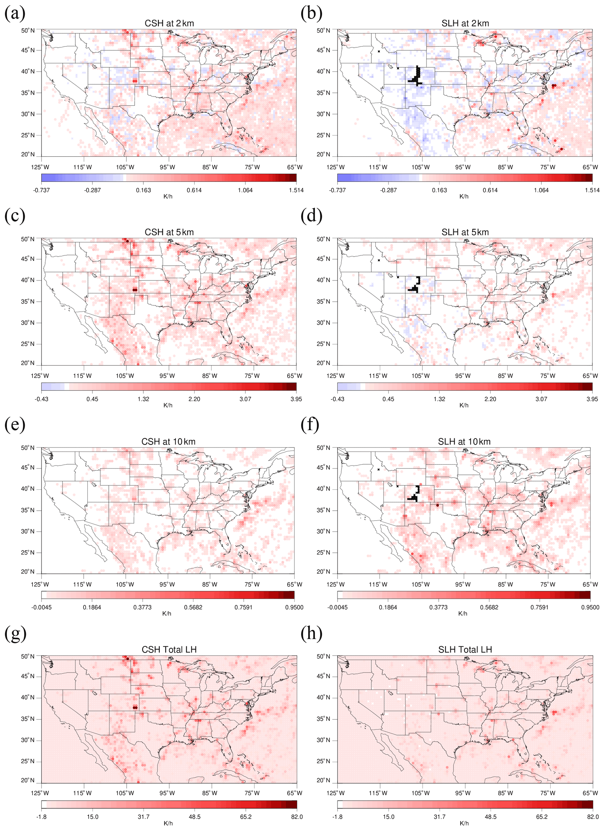
Figure 1 Monthly gridded LH from CSH at (a) 2 km, (c) 5 km, and (e) 10 km; (g) vertically integrated LH from CSH and LH from SLH at (b) 2 km, (d) 5 km, and (f) 10 km; (h) vertically integrated LH from SLH.

Orbital data for these products are provided at the pixel scale (5 km), and although results may be interpreted as “instantaneous” LH, the temporal resolution from low-Earth orbit is too coarse to have much impact on regional forecast models that are initialized hourly if not more frequently.

2.3 LH from NEXRAD

In the operational HRRR model, LH profiles retrieved using radar reflectivity replace modeled LH profiles, which helps initiate convection at the appropriate locations. LH profiles in this case are constructed using a simple empirical formula that converts radar reflectivity to LH. In Eq. (2), reflectivity is converted to potential temperature tendency using a model pressure field. This equation is only applied when radar reflectivity exceeds 28 dBZ. The threshold of 28 dBZ was chosen based on the effectiveness of adding heating from reflectivity in HRRR (Bytheway et al., 2017).

$$\begin{array}{}\text{(2)}& \begin{array}{rl}{T}_{\mathrm{ten}}& ={{\displaystyle \frac{\mathrm{1000}}{p}}}^{R_{\mathrm{d}}/c_{\mathrm{pd}}}{\displaystyle \frac{(L_{\mathrm{v}}+L_{\mathrm{f}})Q_{\mathrm{s}}}{n•c_{\mathrm{pd}}}}\mathrm{where}{Q}_{\mathrm{s}}\\ & =\mathrm{1.5}\times {\displaystyle \frac{{\mathrm{10}}^{z/\mathrm{17.8}}}{\mathrm{264083}}}\end{array},\end{array}$$

where z is the grid radar and lightning proxy reflectivity; T_ten is the temperature tendency; p is the background pressure (hPa); R_d is the specific gas constant for dry air; c_pd is the specific heat of dry air at constant pressure; L_v is the latent heat of vaporization at 0 ^∘C; L_f is the latent heat of fusion at 0 ^∘C; and n is the number of forward-integration steps of digital filter initialization. T_ten in Eq. (2) is produced in K s⁻¹ to meet the needs during the short-term forecast. Although heating rate is not a general output of the forecast model, it is calculated at every time step by dividing the temperature change from the microphysical scheme by the time step, which is usually on the order of few tens of seconds. Therefore, this empirical formula is developed to produce LH consistent with the model framework so that added LH does not produce computational instabilities when ingested.

3 LH profiles from GOES-16

The current operational geostationary satellite, GOES-16, carries the ABI, an instrument with 16 VIS and IR channels. Mesoscale sectors, which are manually selected to observe important weather events, provide data in one-minute intervals. Such high temporal-resolution data have helped observe cloud development in more detail. Using this high temporal-resolution ABI data, convective clouds are detected, and LH profiles for the detected clouds are assigned from an LUT. The LUT is created by running weather research and forecasting (WRF) model simulations. While the CSH and SLH algorithms look for LH profiles in a model-based LUT according to precipitation type and precipitation top height, the LUT for GOES-16 ABI is created for convective clouds that appear bright and bubbling from ABI according to brightness temperature (T_b) at channel 14 (11.2 µm), which is a good indicator of cloud top temperature. LH is not assigned for stratiform clouds from GOES-16, as LH from stratiform clouds is not usually used to initiate convection in the forecast model. Once convective clouds are detected using temporal changes in reflectance and T_b, the LH profile corresponding to the T_b of the detected cloud is assigned from the LUT.

3.1 Definition of convection in model simulations and GOES-16 ABI

In order to make an LUT for LH profiles of convective clouds, convective grid points need to be defined in the model simulation. Convection can be defined in several different ways depending on the variables available, but the most direct and accurate way of defining it is to use vertical velocity (Zipser and Lutz, 1994; LeMone and Zipser, 1980; Xu and Randall, 2001; Houze, 1997; Steiner et al., 1995; Del Genio et al., 2012; Wu et al., 2009). Steiner et al. (1995) and Houze (1997) suggested that convective regions tend to have vertical velocity greater than 1 ms⁻¹, and many previous studies that used vertical velocity to define convection used a threshold of 1 ms⁻¹ (LeMone and Zipser, 1980; Xu and Randall, 2001; Wu et al., 2009). Similarly, this study uses a vertical velocity threshold to define the convective core, as it is one of the prognostic variables in the model simulations. However, in this study, a vertical velocity threshold is defined at the layer of maximum hydrometeor contents. This is intended to exclude potentially high values of negative vertical velocity that can occur at high levels in the cloud if evaporative cooling is present.

To establish the vertical velocity threshold in this study, several values are tested in order to match the convective fraction seen in the GOES-16 convection detection algorithm (described in Lee et al., 2021). The vertical velocity threshold whose convective fractions compared best to GOES-16 is chosen. The GOES-16 convection detection algorithm uses mesoscale sector data with one-minute intervals to detect convective regions from ABI imagery. Two separate detection methods are proposed: one for vertically growing clouds in their early stages, and one for mature convective clouds that move rather horizontally once they reach the tropopause and that often have overshooting tops. A detailed description of the methods can be found in Lee et al. (2021), but it is briefly explained here. The method for vertically growing clouds focuses on T_b decreases over 10 min for two water vapor channels. If the decrease is greater than the designated threshold (−0.5 K min⁻¹ for channel 8 and −1.0 K min⁻¹ for channel 10), it classifies the pixel as convective. For mature convective clouds, the method looks for grid points that have continuously high reflectance (reflectance greater than 0.8), low T_b (T_b less than 250 K), and lumpy cloud top (horizontal gradient values between 0.4 and 0.9) over 10 min. Lumpiness of the cloud top is calculated using the Sobel operator, which is commonly used for edge detection. These thresholds are chosen based on one month of data compared to “PrecipFlag” from the Multi-Radar Multi-Sensor System (MRMS), which classifies precipitation types by combining data from ground-based radar and rain gauge observations. Combining the two methods yielded false alarm rates of 14.4 % and a probability of detection of 45.3 % against the ground-based radar product, but 96.4 % of the false alarm cases were at least raining. Combining the two methods provides results comparable to the radar product, and these methods are rather simple and fast. These methods detect any type of convective region, and therefore, the analysis is conducted without distinguishing different types of convective clouds.

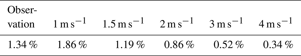
Table 1 shows convective fractions using the GOES-16 convection detecting algorithm and using different vertical velocity thresholds in the model outputs. Using higher thresholds can eliminate non-convective grid points, but at the same time, it will only include the strongest parts of the convective regions. Using a 1.5 m s⁻¹ threshold shows a fractional area closest to the observed fraction; therefore, 1.5 m s⁻¹ is used to define convection in the model output. This number is similar to values used in some previous modeling studies (1 m s⁻¹ in LeMone and Zipser, 1980; Xu and Randall 2001; Wu et al., 2009) and in a satellite-based study (2–4 m s⁻¹ in Luo et al., 2014).

Table 1 Fraction of convective area from observations and using different vertical velocity thresholds in the model output.

3.2 Model simulations used to create a lookup table

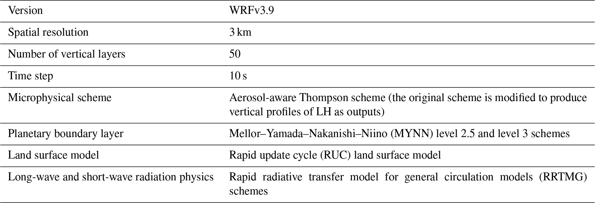
Eleven convective cases are simulated using WRF to obtain enough samples to populate each cloud top temperature bin. The convective cases were chosen over CONUS within the NEXRAD network during May to August in 2017 and 2018. All simulations use the same configuration, shown in Table 2, and HRRR analysis data are used for initial and boundary conditions. All the convective cases are run from the start of any convective activity in the scene for at least several hours, depending on the longevity of convection in each case, and model outputs are collected every 10 min so that the LUT includes LH profiles at all stages and types of convection. However, the LUT is not divided into different types of convection, as it is hard to distinguish convective types from observations. One thing to note is that the magnitude of LH can vary depending on the model configuration, such as spatial resolution, time step, and microphysical scheme. This study uses the same model configuration as the HRRR model for all simulations, which avoids discrepancies in magnitude between the modeled LH and the derived LH that will be inserted into the forecast models. T_bs at 11.2 µm are calculated using the Community Radiative Transfer Model (CRTM). In each scene, convective grid points are defined by the threshold established in the previous section (1.5 m s⁻¹), and LH profiles from the convective grid points with the same T_b from channel 14 are averaged to produce mean profiles for each T_b bin of the LUT. LH profiles included in the LUT are provided in K s⁻¹, as for NEXRAD.

Table 2 Table for WRF simulation setup.

3.3 Mean LH profiles according to cloud top temperature

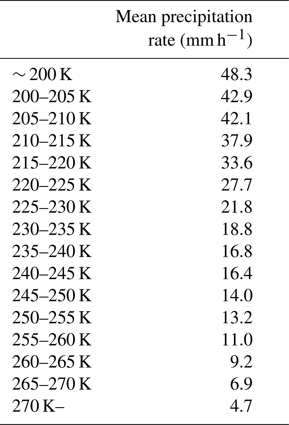
LH profiles of convective clouds from 11 WRF simulations are sorted into 16 bins based on the cloud top temperature at 11.2 µm. The 16 bins range from below 200 K to above 270 K, with a bin size of 5 K. Figure 2 shows the mean vertical profiles of LH in each bin. All profiles exhibit slightly negative LH near the ground due to evaporation, but positive LH is shown at most layers. It is also clear in the figure that, as the T_bs decreases, the profile stretches up in the vertical. Interestingly though, the maximum heating rate is not perfectly proportional to T_b. Considering the maximum LH that is allowed in the HRRR model, which is 0.01 K s⁻¹, these values seem quite reasonable. Table 3 shows the mean surface precipitation rate for each bin. The precipitation rate is inversely proportional to T_b in Table 3. This is expected, as deeper and higher clouds tend to precipitate more. This provides more evidence that mean LH profiles for each bin can reasonably be obtained from GOES-16.

Figure 2 Mean vertical profiles for each cloud top temperature bin.

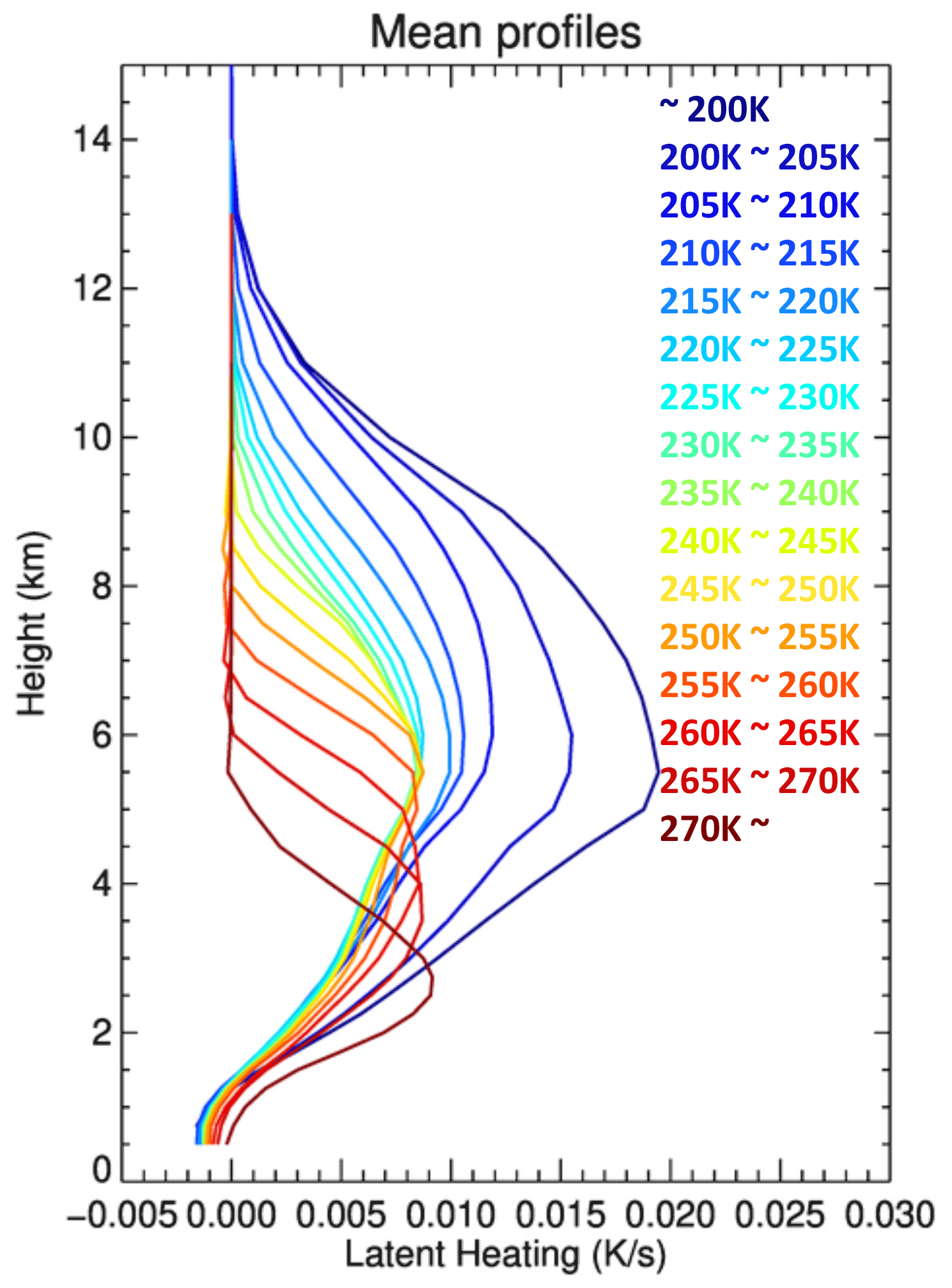
Table 3 Table of mean precipitation rate for each cloud top temperature bin.

The LUT in Fig. 2 is used throughout the later sections, but it can be further divided with additional inputs. A decrease in the brightness temperature is one of the options, but it is not considered in this study for several reasons. Since clouds move over time, cloud advection adds uncertainty to the change in brightness temperature if calculated per pixel. To measure a robust brightness temperature decrease, the decrease can be calculated per cloud and not per pixel. However, LH profiles would have to be assigned for each cloud, and the assigned profile would be inconsistent with the observed cloud top temperature for each pixel. Therefore, using brightness temperature decreases as additional inputs to the LUT is not included in this study, and it remains a topic of inquiry for future studies. Instead, each cloud top temperature bin can be further divided according to composite radar reflectivity, and the additional LUT is presented in Appendix A. Composite reflectivity, if available, can be used to adjust the maximum intensity of LH profiles, as the SLH algorithm adjusts the amplitude by multiplying P_s and P_f. Although it is challenging to get the full vertical profile of radar reflectivity from GOES-16 data, there are algorithms developed to estimate composite reflectivity from GOES-16, such as GOES Radar Estimation via Machine Learning to Inform NWP (GREMLIN; Hilburn et al., 2021). Therefore, this additional LUT could be used along with such an estimator to assign LH profiles in more detail, but it is not used further in this study.

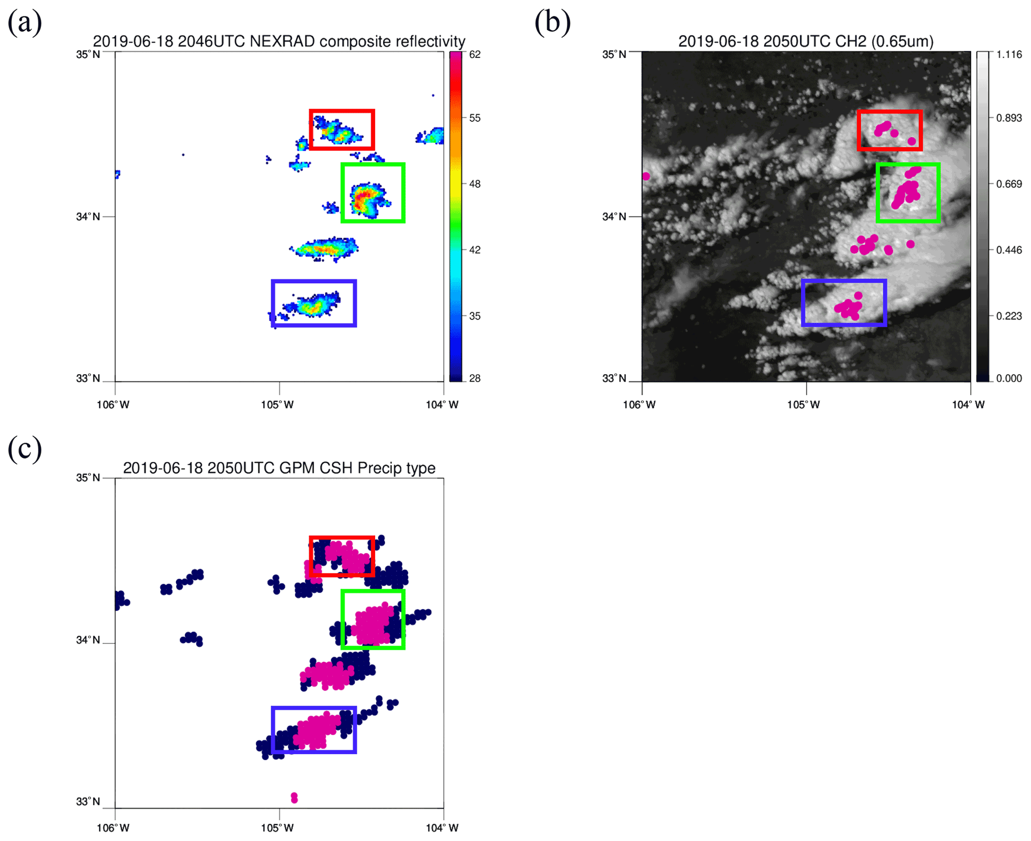
Figure 3 A scene on 18 June 2019. (a) NEXRAD composite reflectivity; only the regions with reflectivity greater than 28 dBZ are shown in colors; color bar is in dBZ. (b) Convective regions detected by GOES-16 are colored in pink on top of GOES-16 visible imagery of channel 2 (0.65 µm) reflectance. (c) Precipitation type defined by CSH; convective regions are colored in pink, while stratiform regions are colored in navy.

4 Comparisons of LH profiles between GPR DPR, NEXRAD, and GOES-16 ABI

4.1 A case study on 18 June 2019

LH from three different instruments – GOES-16 ABI, NEXRAD, and GPM DPR – are examined in this section. Methods using GOES-16 and DPR products are similar in the sense that they use cloud top height or PTH to look for mean profiles in the LUT created with model simulations, although DPR has additional parameters such as surface rain rate, which is used to vary the magnitude of the heating rate. In contrast, NEXRAD uses an empirical formula to convert radar reflectivity to LH regardless of PTH. They are all instantaneous heating but are provided in different units. LH from GOES-16 and NEXRAD are in K s⁻¹ to easily match with modeled heating rate, while DPR products are in K h⁻¹. Therefore, LH in K h⁻¹ from DPR products are converted to K s⁻¹ for comparison.

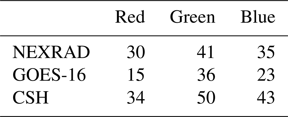
A scene from 18 June 2019 is shown in Fig. 3 to compare the precipitation types (convective or stratiform) of the three products, as this is one of the major factors in estimating LH profiles. The regions with reflectivity greater than 28dBZ in Fig. 3a are regions where LH is estimated from NEXRAD reflectivity to be used in HRRR but not necessarily convective regions. Pink regions on top of the visible image at channel 2 (0.65 µm) in Fig. 3b are convective regions detected by GOES-16, and they represent the smallest convective areas relative to the other two methods. The number of convective grid points from each product after interpolating into the 3km-resolution WRF grid is presented in Table 4 for a quantitative comparison. Even though areal coverage differs by the methods, the locations of the convective cores matches well between the products.

Table 4 Total number of grid points from NEXRAD, GOES-16, and CSH in the red, green, and blue box regions after interpolating into the same 3 km WRF grid.

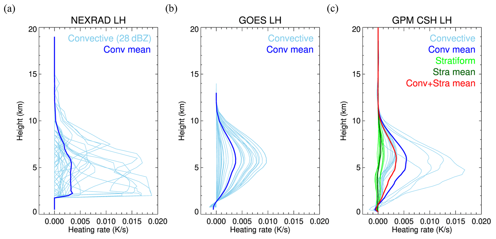
Clouds in the colored boxes in Fig. 3 are all convective clouds but in different evolutional stages. Clouds in red, green, and blue boxes have high, low, and mid-level cloud top temperature, respectively. Since the three products have different spatial resolutions, LH profiles from NEXRAD, GOES-16, and CSH for these clouds are interpolated into the same WRF grid with a 3 km resolution for a direct comparison in Figs. 4, 5, and 6. CSH provides LH for both convective and stratiform regions; thus, the different colors of the lines in Figs. 4c, 5c, and 6c represent different cloud types. Lines with a light blue color are LH profiles of convective grid points, while the blue line is the mean of these profiles. Similarly, LH profiles of each stratiform gird point are in light green, while the mean of these profiles is in dark green. The mean of all LH profiles is colored in red. Convective LH profiles from CSH show heating throughout the vertical layers, as expected, except near the surface due to evaporation at lower levels. LH profiles in stratiform regions show cooling at low levels below a melting level and heating at levels above. LH profiles from GOES-16 (GOES LH) corresponding to the three convective clouds are shown in Figs. 4b, 5b, and 6b. When GOES LH and CSH are compared, the mean profile of convective LH from CSH (Figs. 4c, 5c, and 6c) is similar to GOES LH in blue (Figs. 4b, 5b, and 6b), both in terms of the magnitude and the vertical shape.

In contrast, LH from NEXRAD (NEXRAD LH) shows a different vertical profile than GOES LH and CSH, which both use the LUT consisting of model simulations. GOES LH and CSH peak around the middle of the atmosphere, while the NEXRAD LH in the convective core tends to peak at low levels where radar reflectivity is high (Figs. 4a, 5a, and 6a). At low levels where model simulations have cooling, NEXRAD LH does not show cooling due to Eq. (2), which is designed to only produce positive values. This heating at lower levels induces convergence in the lower atmosphere and divergence in the upper atmosphere, and thus, convection can be effectively initiated from the added heating.

Although their vertical shapes are different, the magnitude of the NEXRAD LH is similar to the other products. Overall values of the mean convective LH profiles from NEXRAD in blue are slightly smaller than the mean convective profile of GOES LH and CSH (blue line) but are closer to the total mean profile of CSH (red line), which indicates that the 28dBZ threshold might include some stratiform regions as well. The smaller mean of the NEXRAD LH is mainly attributed to anvil regions where reflectivity is greater than 28 dBZ, which only exist at a few vertical layers, with reflectivity being equal to 0 dBZ elsewhere.

Even though the mean NEXRAD LH is smaller, the total LH for the region can be similar when it is summed up over the region due to the broader area determined by the threshold of 28 dBZ in Fig. 3a relative to that of GOES-16 (Fig. 3b). Therefore, the total LH of each cloud is again compared between the three products (Table 5). Here, “total LH” is defined as the vertically and horizontally integrated LH over each convective cloud. This comparison is intended to account for differences in the area and for convective definitions that make direct comparison between vertical levels difficult. In addition, comparing combined values will be meaningful, as those are the values that will be used to initiate each convective cloud. Table 5 shows that the total LH from CSH tends to be higher than that from the other two products, while the total LH is shown to be similar between NEXRAD and GOES-16, although GOES LH is slightly larger. Despite the smaller mean of NEXRAD LH that was shown in Figs. 4, 5, and 6, it shows a good agreement with GOES LH in total heating.

4.2 Three-month analysis against NEXRAD LH

The case study from Sect. 4.1 is presented to show how the vertical structure of GOES LH compares to other radar products. In this section, three months of data from May, June, and July of 2020 are used to compare total LH for convective clouds between GOES-16 and NEXRAD. Total LH used in this section is, again, vertically and horizontally integrated over each convective cloud. Both GOES-16 brightness temperature and NEXRAD reflectivity are resampled to the 3 km HRRR grid for a direct comparison and are compared under several conditions that the HRRR model uses to avoid disruption in the existing model physics. During the convective initiation step in the HRRR model, LH is calculated from NEXRAD radar reflectivity following Eq. (2) if the layer is cloudy, is under the GOES cloud top (using level 2 cloud top pressure data), is above the planetary boundary layer, and has a temperature less than 277.15 K. Additionally, LH is calculated for temperatures greater than 277.15 K only if the corresponding reflectivity exceeds 28 dBZ.

GOES LH is calculated with the same criteria described above, except for the additional 28 dBZ categorization. Adjacent convective grid points by the detection algorithm are clustered to define a convective cloud. In order to minimize errors coming from different definitions of convection in GOES and NEXRAD, total LH is compared only in clouds where both NEXRAD and GOES detect convection. Since the area defined as convective cloud tends to be wider in NEXRAD than in GOES-16 and since one convective cloud from NEXRAD tends to include multiple convective cloud systems defined by GOES, the comparison is done by combining all convective clouds from GOES-16 that overlap with each convective cloud by NEXRAD. Regions with low radar quality, as indicated by the radar quality flag, are excluded in the analysis.

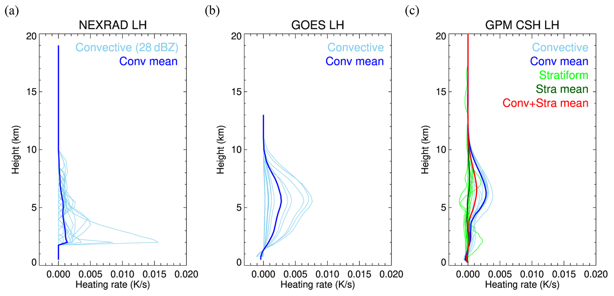
Figure 4 LH profiles from (a) NEXRAD, (b) GOES-16, and (c) CSH for the red box region. Light blue lines are each the LH profile for individual convective grid points, and the darker blue line is a mean profile of the light blue lines. In (c), the LH profile for each stratiform grid point is colored in light green, and its mean profile is colored in dark green. The mean of all (convective and stratiform) LH profiles for CSH is colored in red.

Figure 5 Same as Fig. 4 but for the green box region.

Figure 6 Same as Fig. 4 but for the blue box region.

Among the 4045 convective clouds collected during the three months of the analysis, only 2660 convective clouds are within reasonable range of each other in both GOES-16 and NEXRAD. Here, we define “reasonable range” as follows: the number of convective grid points from GOES-16 does not exceed 5 times that of NEXRAD, and vice versa. A total of 2660 clouds are selected, and the total LH for these clouds from both GOES-16 and NEXRAD is fitted to a linear regression model. Figure 7 shows a scatter plot of NEXRAD LH and GOES LH for each convective cloud using log–log space. A decent correlation coefficient of 0.83 is obtained between NEXRAD LH and GOES LH in Fig. 7. In most cases, large discrepancies in total LH seem to be caused by a corresponding discrepancy in the number of convective grid points, which is inevitable, but overall, the total LH values seem to agree well if the number of convective grid points is similar.

Table 5 Total LH (K s⁻¹) from NEXRAD, GOES-16, and CSH in the red, green, and blue box regions.

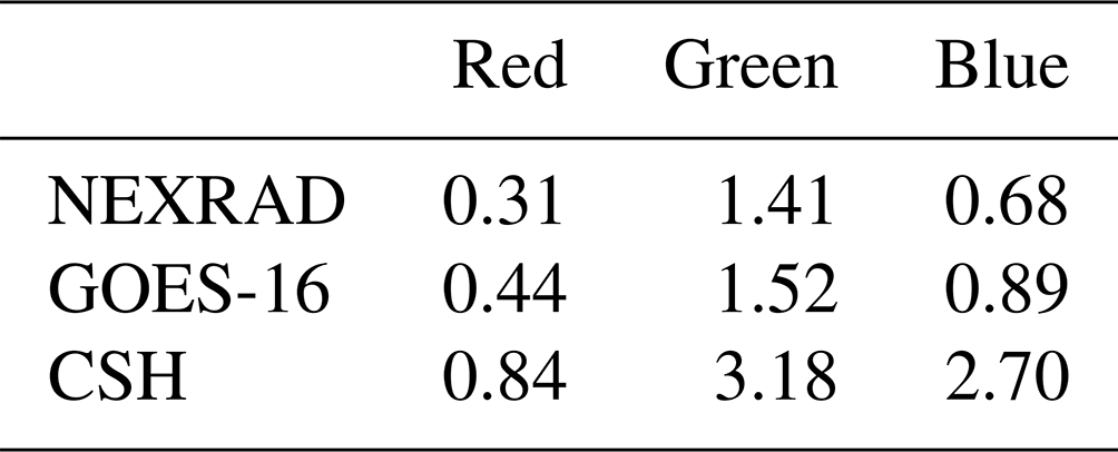
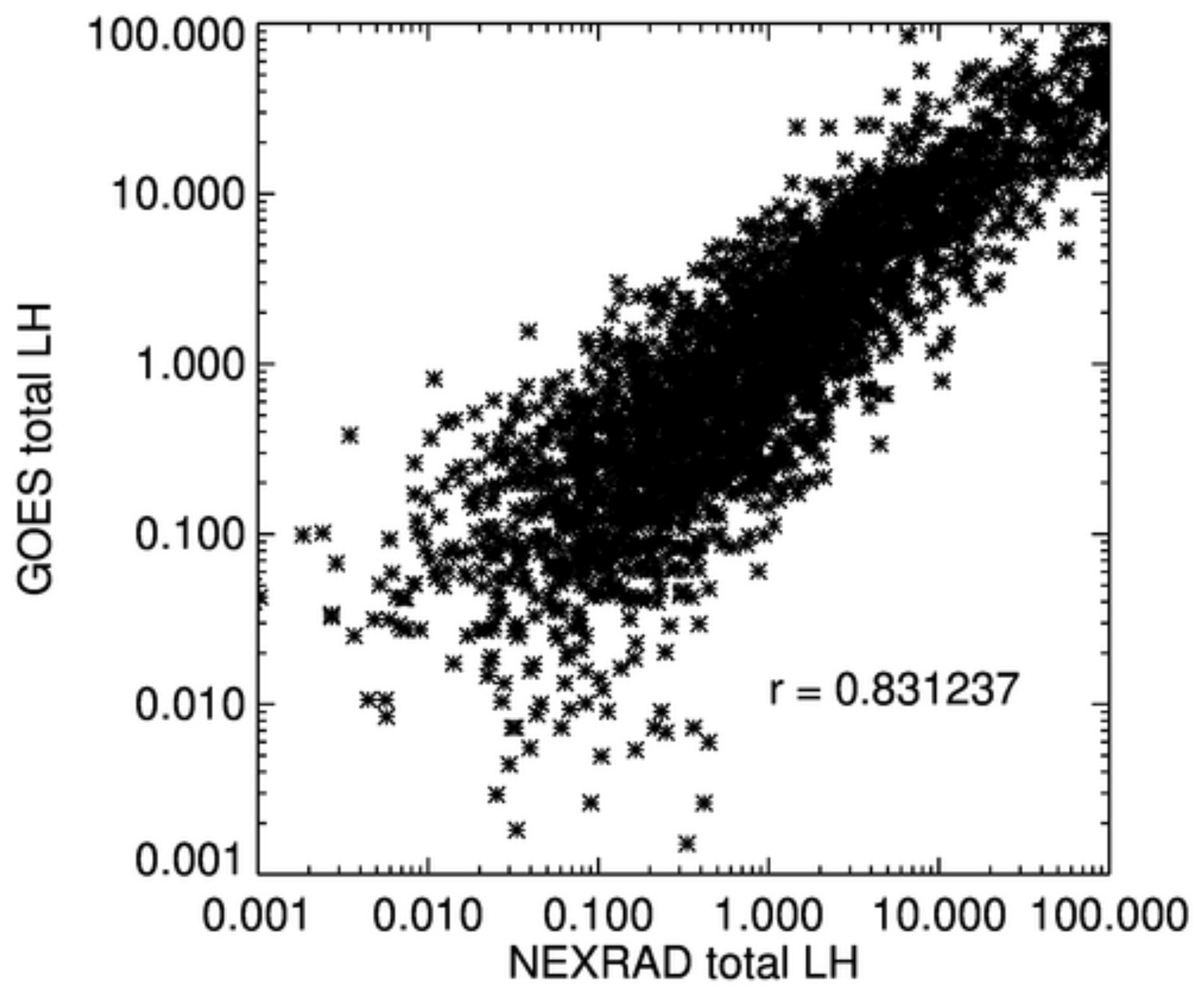
Figure 7 Scatter plot of NEXRAD total LH and GOES total LH in K s⁻¹. It is plotted in log–log axes.

5 Impacts of NEXRAD LH and GOES LH on precipitation forecast

The WRF model was run for one convective case on 10 July 2019 to compare the impacts of GOES LH and NEXRAD LH on precipitation forecasts. HRRR data are used as initial and boundary conditions, and the same configuration is used as when making the LUT. GOES-16 visible data are only available for initialization from 15:00 to 22:00 UTC, so results are compared after one hour of running freely, from 17:00 to 00:00 UTC. In order to initiate convection in the same manner as HRRR does with NEXRAD, modeled LH profiles are replaced with the observed LH profiles at every time step during the one hour of the pre-forecast period. Observed LH profiles at 45, 30, 15, 0 min before the start of the free run are used for their respective 15 min period before the start of the free run. After the pre-forecast run, the model is run freely for an hour, and after the one-hour free run, the one-hour accumulated rainfall rate results are compared. One-hour rain accumulation from simulations without using any observed LH (CTL), using NEXRAD LH (NL), and using GOES LH (GL) are validated against gauge bias-corrected quantitative precipitation estimation (QPE; one-hour accumulation) from MRMS.

Figure 8 shows one simulation where observed LH is applied from 15:00 to 16:00 UTC, after which the model is freely run for an hour until 17:00 UTC. The CTL run (Fig. 8a) misses many convective regions, and precipitation is markedly less than MRMS observations in Fig. 8b. Both the NL and GL runs initiated convection in the right place and enhance precipitation. In the light green box region where the CTL run totally misses convection, NL and GL runs both produce precipitation, although there is an overestimation of precipitation in the NL run and an underestimation in the GL run. In the dark green box region where convection is weak in the CTL run, the NL and GL runs increased precipitation amounts closer to the observations. The NL run correctly initiates convection in the yellow box region but not in the red box region, while the GL run correctly initiates convection in the red box but not in the yellow box.

Figure 8 One-hour rain accumulation at 17:00 UTC on 10 July 2019 from (a) a simulation without any LH observation, (b) MRMS gauge-corrected quantitative precipitation estimation (QPE), (c) a simulation using NEXRAD LH, and (d) a simulation using GOES LH.

These results can be further explained by looking at Fig. 9, which presents maps of vertically integrated NEXRAD LH and GOES LH that are applied to the model at 16:00 UTC (the last time that observed LH profiles are applied during the 15:00–16:00 UTC period). As seen in the enlarged two green box regions in Fig. 9, NEXRAD shows very high total LH (up to 0.35 K s⁻¹) in a few grid points and small LH in surrounding areas, while most of the GOES LH values in the two green boxes are at or below 0.2 K s⁻¹. The reason why there was an overestimation of precipitation in the NL run (Fig. 8c) could be due to this extremely high NEXRAD LH. Interestingly, in the red box region, both NEXRAD and GOES have similar total LH values, but only the GL run produced precipitation (in Fig. 8d). Lastly, it makes sense that the GL run did not initiate convection in the yellow box region (Fig. 8d), because no LH is applied due to missed convection by the GOES convection detection algorithm (Fig. 9b). Overall, both NEXRAD LH and GOES LH have positive impacts on the precipitation forecast, and their forecast results appear to have similar skills.

Figure 9 Vertically integrated LH at 16:00 UTC on 10 July 2019 from (a) NEXRAD and (b) GOES-16. Two green box regions are enlarged for better comparison.

For a quantitative evaluation, fraction skill scores (FSS) are calculated for the eight simulations that added LH for different one-hour time periods (LH is added for an hour during 15:00–16:00 UTC, 16:00–17:00 UTC..., 22:00–23:00 UTC, and FSS are calculated after the one-hour free run at 17:00, 18:00,..., 00:00 UTC). FSS is one of the neighborhood-based precipitation verification metrics introduced by Roberts and Lean (2008), and it is calculated using Eq. (3):

$$\begin{array}{}\text{(3)}& {\mathrm{FSS}}_{\left(n\right)}=\mathrm{1}-{\displaystyle \frac{\frac{\mathrm{1}}{N_x{N}_y}\sum _{i=\mathrm{1}}^{N_x}\sum _{j=\mathrm{1}}^{N_y}{\left[O_{i,j}-P_{i,j}\right]}^{\mathrm{2}}}{\frac{\mathrm{1}}{N_x{N}_y}\left[\sum _{i=\mathrm{1}}^{N_x}\sum _{j=\mathrm{1}}^{N_y}{O}_{i,j}^{\mathrm{2}}+\sum _{i=\mathrm{1}}^{N_x}\sum _{j=\mathrm{1}}^{N_y}{P}_{i,j}^{\mathrm{2}}\right]}},\end{array}$$

where N_x and N_y are the number of columns and rows, and O_i,j and P_i,j are, respectively, an observed and model forecast fraction calculated over a small n×n domain. It calculates a fraction that passes a threshold value over an n×n domain, and the fraction over the small domain is compared rather than individual grid points. In this study, a 15 km × 15 km domain is used to calculate FSS for the six one-hour accumulated precipitation thresholds of 0.254, 2.54, 6.35, 12.7, 25.4, and 50.8 mm h⁻¹ (0.01, 0.1, 0.25, 0.5, 1, and 2 inch h⁻¹).

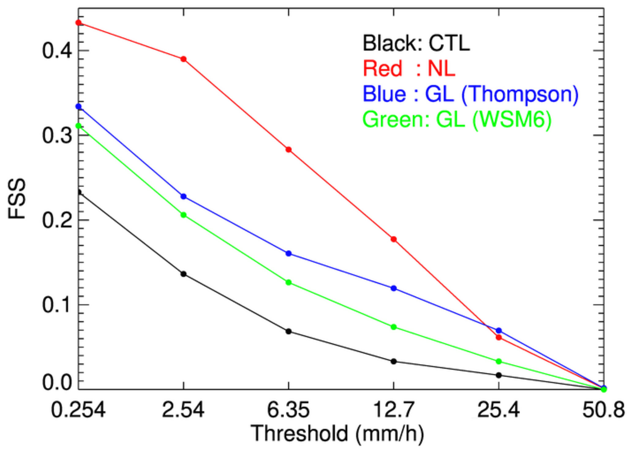
Figure 10 Fraction skill score (FSS) using thresholds of 0.254, 2.54, 6.35, 12.7, 25.4, and 50.8 mm h⁻¹ (0.01, 0.1, 0.25, 0.5, 1, and 2 inch h⁻¹) for CTL (black), NL (red), GL with the Thompson scheme (blue), and GL with WSM6 scheme (green) runs.

The overall FSS for the four simulations is shown in Fig. 10. Black, red, blue, and green lines represent CTL, NL, GL with the Thompson scheme, and GL with the WSM6 scheme, respectively. Compared to the CTL, both the NL and GL runs show significant improvements in FSS for all thresholds. Although the NL run outperforms GL at smaller thresholds, the GL run shows better results at higher thresholds of 25.4 and 50.8 mm h⁻¹. This can be because GOES LH tends to have maximum heating in the middle atmosphere, which can develop deeper clouds, but further investigation is needed to study the sensitivity of different vertical profiles to precipitation forecasts. An additional GL run, using the different microphysical scheme of WSM6, is provided to briefly show the impacts of different microphysical schemes. It has less positive impacts, indicating that maintaining consistency in the microphysical scheme could be critical. Nonetheless, it shows that LH from GOES-16 presented in this study can be useful for improving precipitation forecasts, especially in the regions where ground-based radar data are not available.

6 Conclusions

A method to obtain vertical profiles of LH from GOES-16 ABI data was described. Convective clouds are first detected using temporal changes in reflectance and T_b, and then LH profiles for the detected cloud are found by searching for an LUT created using WRF model simulations. The LUT contains LH profiles of convective clouds that are defined by a threshold of 1.5 m s⁻¹ for the modeled vertical velocity, and these convective LH profiles are sorted according to T_b at 11.2 µm, which is a good indicator of cloud top height. Mean profiles that represent each T_b bin show good correlation with cloud top temperature, with lower T_b bins having deeper LH profiles. Precipitation rates corresponding to each bin are also well correlated to T_b. Even though the LUT in Fig. 2 uses one infrared channel to estimate LH profiles, it is actually more than just one brightness temperature value. The GOES-16 convection detection algorithm uses 10 time steps of channel 2 reflectance and channel 8 and 10 brightness temperature data to find active convective regions with a bubbling cloud top and brightness temperature decrease; thus the overall algorithm uses more information than just one brightness temperature value. In addition, LH values in the LUT are well within the range that is allowed in the HRRR model to initiate convection using NEXRAD.

To investigate how LH from GOES-16 differs from other radar products, LH from GOES-16, NEXRAD, and CSH are compared in three convective clouds with different cloud top heights. Vertical profiles of convective LH from GOES-16 are very similar to those from CSH that use model simulations in the LUT. Their vertical profiles show heating throughout the vertical layers, except near the surface, where evaporation occurs, and heating peaks around the middle of the atmosphere. This vertical pattern differs from that of the empirical formulation used with by HRRR the radar reflectivity. Vertical profiles of LH from NEXRAD depend strongly on the vertical profiles of reflectivity, which typically peaks near the surface in convective regions. This leads the NEXRAD maximum LH to be at lower levels, not often simulated in the models.

Even though vertical profiles of LH from the various methods differ, the total LH, which is calculated by integrating the horizontal and vertical LH for each convective cloud, is shown to be similar between GOES-16 and NEXRAD. A three-month analysis shows good correlations overall between GOES-16 and NEXRAD if the detected convection areas are similar. Besides the limitation in convection detection by GOES-16, GOES LH estimates can have large errors in the case of multi-layer clouds or in clouds with sheared structure, as it is based on the cloud top.

In order to examine the impacts of GOES LH compared to NEXRAD LH in precipitation forecast, one case study is presented. Applying LH derived from GOES-16 to model initialization allows for correct initiation of convection in the scene, and the simulation result looks similar to the one derived from applying NEXRAD LH. Although the GOES convection detection algorithm is not perfect and misses some convection, and even though GOES LH is somewhat restricted to cloud top information, these results prove that LH obtained from GOES-16 have reasonable values and can be used to improve precipitation forecasts over the region where ground-based radar data are not available.

This work is a proof-of-concept study to show the potential of using infrared data in initializing convection, and there is room for improvement. The LUT can be improved by adding more input variables, such as cloud top cooling rate. In the case of using cloud top cooling rates as inputs, additional wind products will be needed to remove model and observational errors coming from cloud advection. Aside from changing input variables, other microphysical schemes can be tested for the LUT to compare intensities or vertical structures of the derived LH profiles using different microphysical schemes. Further investigation will also be needed to analyze the impacts of the different vertical structures of LH in convective initiation.

Appendix A

An additional LUT using composite reflectivity along with cloud top temperature is provided here. This LUT can be used with NEXRAD composite reflectivity or with other synthetic radar reflectivity simulators that use GOES-16 data, such as GREMLIN. This LUT includes vertical profiles of mean reflectivity for each cloud top temperature and composite reflectivity bin (Fig. A1) as well as vertical profiles of LH (Fig. A2). Radar reflectivity profiles retrieved using this LUT can be used directly in the model initialization step in the same way as ground-based radar reflectivity profiles are used in the HRRR model, or LH profiles in this LUT can be used with some modifications in the model initialization step, as in this study. Each plot shows the mean profiles for each cloud top temperature bin, while different colors in the plot represent each composite reflectivity bin. Note that, for higher cloud top temperature bins, high composite reflectivity bins (red or brown lines) are not shown, because clouds with warmer cloud tops do not generally show high composite reflectivity. For lower cloud top temperature bins, low composite reflectivity bins (blue lines) are not shown, because deep convective clouds tend to have high composite reflectivity.

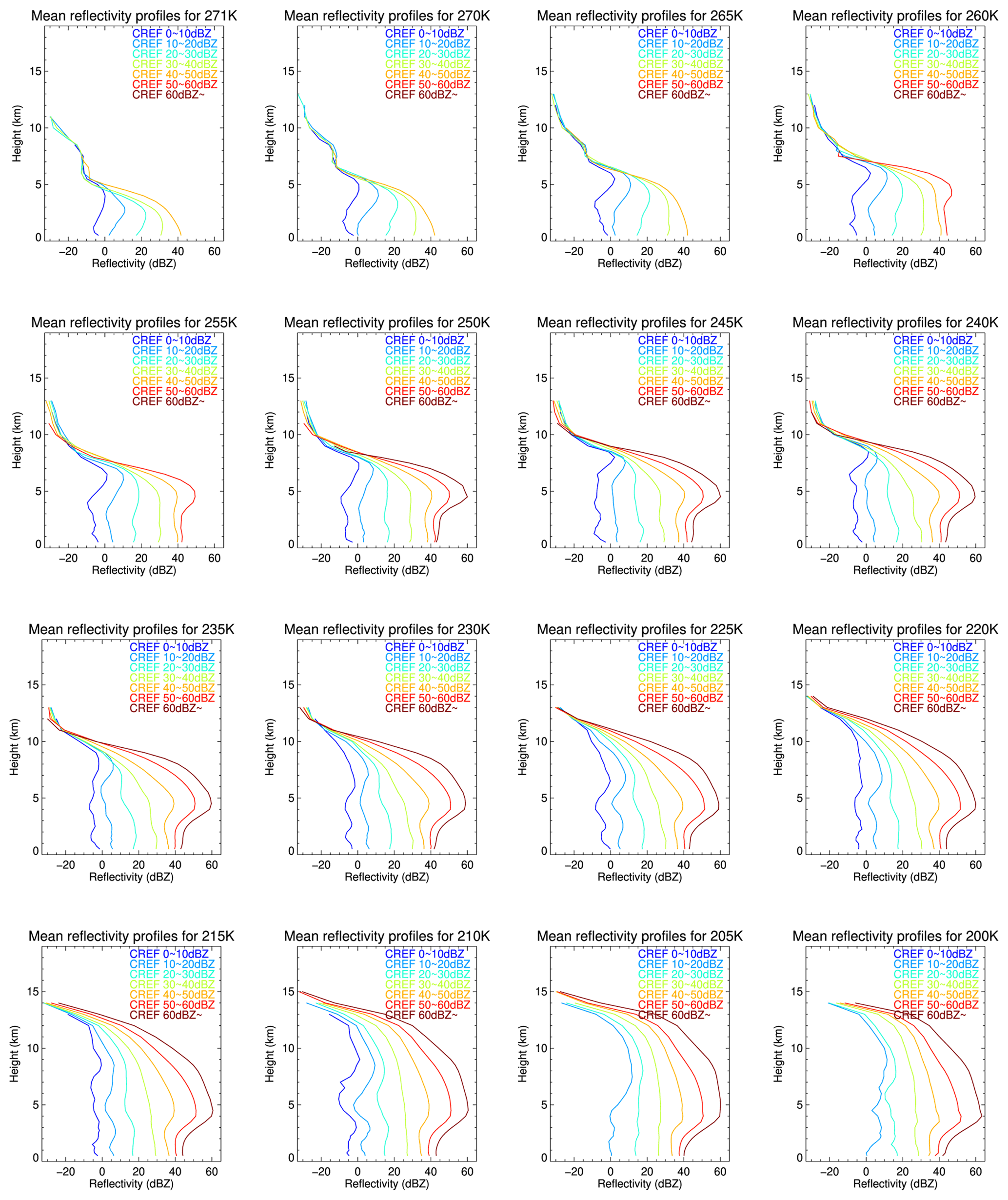
Figure A1 Mean reflectivity profiles for 16 cloud top temperature bins and 7 composite reflectivity bins. Each plot corresponds to each cloud top temperature bin, and different colors in the plot represent each composite reflectivity bin.

Figure A2 Mean LH profiles for 16 cloud top temperature bins and 7 composite reflectivity bins. Each plot corresponds to each cloud top temperature bin, and different colors in the plot represent each composite reflectivity bin.