In situ particle sampling relationships to surface and turbulent fluxes using large eddy simulations with Lagrangian particles

Source functions for mechanically driven coarse-mode sea spray and dust aerosol particles span orders of magnitude owing to a combination of physical sensitivity in the system and large measurement uncertainty. Outside special idealized settings (such as wind tunnels), aerosol particle fluxes are largely inferred from a host of methods, including local eddy correlation, gradient methods, and dry deposition methods. In all of these methods, it is difficult to relate point measurements from towers, ships, or aircraft to a general representative flux of aerosol particles. This difficulty is from the particles' inhomogeneous distribution due to multiple spatiotemporal scales of an evolving marine environment. We hypothesize that the current representation of a point in situ measurement of sea spray or dust particles is a likely contributor to the unrealistic range of flux and concentration outcomes in the literature. This paper aims to help the interpretation of field data: we conduct a series of high-resolution, cloud-free large eddy simulations (LESs) with Lagrangian particles to better understand the temporal evolution and volumetric variability of coarse- to giant-mode marine aerosol particles and their relationship to turbulent transport. The study begins by describing the Lagrangian LES model framework and simulates flux measurements that were made using numerical analogs to field practices such as the eddy covariance method. Using these methods, turbulent flux sampling is quantified based on key features such as coherent structures within the marine atmospheric boundary layer (MABL) and aerosol particle size. We show that for an unstable atmospheric stability, the MABL exhibits large coherent eddy structures, and as a consequence, the flux measurement outcome becomes strongly tied to spatial length scales and relative sampling of crosswise and streamwise sampling. For example, through the use of ogive curves, a given sampling duration of a fixed numerical sampling instrument is found to capture 80 % of the aerosol flux given a sampling rate of $zf/w_{\ast }\sim$ 0.2, whereas a spanwise moving instrument results in a 95 % capture. These coherent structures and other canonical features contribute to the lack of convergence to the true aerosol vertical flux at any height. As expected, sampling all of the flow features results in a statistically robust flux signal. Analysis of a neutral boundary layer configuration results in a lower predictive range due to weak or no vertical roll structures compared to the unstable boundary layer setting. Finally, we take the results of each approach and compare their surface flux variability: a baseline metric used in regional and global aerosol models.

1 Introduction

Aerosol particles in the atmosphere contribute to environmental processes related to cloud physics, radiative forcing, and geochemical cycles. Coarse- and giant-mode sea salt and sea spray particles affect the mass, momentum, and energy exchange between the atmosphere and ocean (Lewis and Schwartz, 2004; Veron, 2015) based on their diameter, total mass, and composition. Sea spray can be equally as important as fine-mode aerosol particles for indirect effects (Jensen and Lee, 2008), can perturb radiation budgets in the visible and infrared (Hulst and van de Hulst, 1981), and can even impact latent heat transport within the marine boundary layer (Fairall et al., 1994; Andreas et al., 2015). These aerosol particles may also contribute to air pollution through new particle formation (Lee et al., 2019; Wu et al., 2021) and inhibit lightning frequency (Pan et al., 2022). Despite their importance and extensive study, sea salt and spray physics remain poorly quantified, as a large range of uncertainty in their spatiotemporal distribution continues to be observed in models and field observations (Bian et al., 2019; Watson-Parris et al., 2019); similar large uncertainty extends to any mechanically generated coarse- or giant-mode aerosol species, such as dust. These large uncertainties are due to the strong physical sensitivities of mechanically generated aerosol particles to their surface and surface layer turbulent properties as well as large length scale and timescale histories of atmospheric turbulence that local measurements do not necessarily capture.

The beginning of the primary marine aerosol (PMA) life cycle process is particle generation by the entrainment of air into water from breaking waves, the formation of bubble rafts, and subsequent bubble bursting with the formation of film and jet drops (Monahan et al., 1986; de Leeuw et al., 2011; Lewis and Schwartz, 2004; Veron, 2015). Larger droplets, known as spume, can also be torn from breaking waves. Known as the sea spray generation function (SSGF), the rate of aerosol loading into the atmosphere has persisted with high uncertainty, especially for large droplets and aerosols. Thus, the SSGF is an active area of research, as breaking waves (Toba and Chaen, 1973; Wu, 1992) and surface–bubble dynamics (Keene et al., 2017; Deike et al., 2018) are examples of the large number of air–sea processes that challenge an accurate SSGF quantification (Sutherland and Melville, 2015). Indeed, large differences persist between measurement datasets (e.g., Andreas, 1998; Lewis and Schwartz, 2004; Reid et al., 2006; Grythe et al., 2014). Fundamental measurements have also been questioned with the use of different instrumentation (stationary flux towers, airborne measurements, lidars, ships, differing in situ probe and/or measurement types), which have led to persistently uncertain concentrations and/or size-dependent profiles within field observational studies (Blanchard et al., 1984; Porter and Clarke, 1997; Reid et al., 2006). Even the methods of flux calculations themselves are highly varied, ranging from local correlations and vertical profiles to box model approaches and eddy correlation – each with their advantages and disadvantages (see, e.g., the review by Lewis and Schwartz, 2004). When these flux deductions are then applied in models, the models might then propagate incorrect forecasting and prediction of their spatiotemporal distribution. Thus, a biased SSGF (or any other aerosol source function) may improve or diminish model skill independent of the flux parameter's true skill (see, e.g., the discussion in Sessions et al., 2015). There are numerous factors that are hypothesized and still debated as to SSGF dependencies that may account for some of the differences in the literature and with ongoing field research, including wave state, sea surface temperature, atmospheric stability, and biological activity including diurnal effects (e.g., Irwin and Binkowski, 1981; Kapustin et al., 2012; Grythe et al., 2014; Keene et al., 2017; Srivastava and Sharan, 2017).

As a case in point, the NASA Cloud, Aerosol, Monsoon Processes Philippines Experiment (CAMP2Ex) P3 aircraft and Office of Naval Research Propagation of Intraseasonal Oscillations (PISTON) R/V Sally Ride tried to quantify both turbulence and aerosol properties over the Sulu Sea and subtropical western Pacific (WESTPAC) within the Maritime Continent's boreal summertime southwest monsoon. Like many other field-based studies (Lauros et al., 2011; Li et al., 2017), these platforms have obtained the vertical distribution of aerosol particles in the marine atmospheric boundary layer (MABL) (Blanchard et al., 1984; de Leeuw, 1986; Gong et al., 1997; Reid et al., 2001). Both the P3 and the R/V Sally Ride made point or curtain measurements of atmospheric aerosol and turbulence properties from which aspects of the aerosol life cycle are hoped to be inferred, including source functions and particle lifetimes. However, such measurements represent a small set of parcels that have both local and long-range aerosol influences: from individual gust fronts to as far away as the Indian Ocean (Reid et al., 2013, 2015). Sea salt data in particular are difficult to interpret due to both measurement shortcomings and the nature of MABL flows (e.g., Reid et al., 2006). Therefore, when the P3 or Sally Ride makes a measurement of sea salt it is often difficult to know what that measurement actually represents.

CAMP2Ex found that the monsoonal MABL is quite heterogeneous, with features such as convergence lines, land breezes, cold pools, and detainment features within a large littoral environment. The observations led this study to hypothesize that MABL heterogeneity is a further complication of SSGF quantification that may also help explain the differences between flux measurements that are likewise overwhelmingly littoral. That is, high volumetric variability and strong gradients within the MABL, ranging from changes in wind along a sampled trajectory over hundreds to thousands of kilometers to scales of the order of 1 km, can lead to further diversity between individual flux measurements. Flux measurement methods assume some form of atmospheric steady state and spatial homogeneity. For example, eddy correlation or vertical profile methods measure the local net flux, which is often assumed to be the total production flux; however, when there are high winds upstream of the measurement point, that may result in a net downward flux even if active but less production is being taken place. Box model methods, whereby upstream and downstream states are measured, likewise measure a net flux, but if regions and conditions are chosen properly, uncertainty in the downward and dry deposition flux can be sequestered (e.g., Reid et al., 2001; Kapustin et al., 2012). Even so, in these, knowledge of the air mass history and an invariant atmospheric structure are assumed. In all cases one must be cognizant of uncertainties associated with high-resolution atmospheric features and their association with the sea spray aerosol distribution, including the state of the surface layer, the presence of MABL roll features and diurnal (i.e., nonstationary) turbulence (e.g., LeMone, 1973; Wurman and Winslow, 1998; Kapustin et al., 2012; Monaldo et al., 2014; de Szoeke et al., 2021; Prajapati et al., 2021), or the prevalence of cold pools (Reid et al., 2015, 2016; de Szoeke et al., 2017).

Examples of a simple and common MABL feature observed as surface winds speeds increase to whitecapping levels are MABL roll structures. During the CAMP2Ex field campaign, the Sentinel-1 synthetic aperture radar (SAR) obtained 20 m resolution imagery over the Sulu Sea on 1 September 2019, as shown in Fig. 1. The Sentinel-1 normalized cross section values were converted to 250 m sampled ocean surface wind speeds using the CMOD4 geophysical model function and wind directions obtained from the Global Forecast System (Monaldo et al., 2013). On this day were typical southwest monsoon conditions with surface wind features ranging from ∼ 5 to 9 m s⁻¹ over an approximately 30 km × 30 km area (see black box in Fig. 1 for scale reference). As mean winds reach 7 m s⁻¹ within a small sector, the surface wind speed minimum and maximum organize along lines ∼ 2 km apart, parallel to the direction of the wind as provided by the ERA5 reanalysis (model summary in Hersbach et al., 2020). The configuration represents the formation of coherent roll structures and vortices in the MABL. In comparison, the ERA5 reanalysis wind speeds (not shown) provide a smooth wind analysis ranging from 5 m s⁻¹ in the lower left corner to 6 m s⁻¹ in the upper right, below the threshold for whitecaps (Monahan et al., 1986; Wu, 1992). This SAR wind imagery demonstrates some of the challenges facing field campaigns: the MABL is not uniform and exhibits horizontal and vertical structure of ranging wind speeds. Instantaneous snapshots by ship or aircraft lead to questions regarding the local representativeness of in situ concentration and fluxes made by ships or aircraft. How does a regional SSGF relate to in situ ship or aircraft measurements? How much sampling (temporally or spatially) is required to achieve convergence between the measurement and regional flux? What are the potential measurement sensitivities to unresolved upstream sea spray production? Are there measurement practices that can aid in the measurement of turbulent aerosol fluxes?

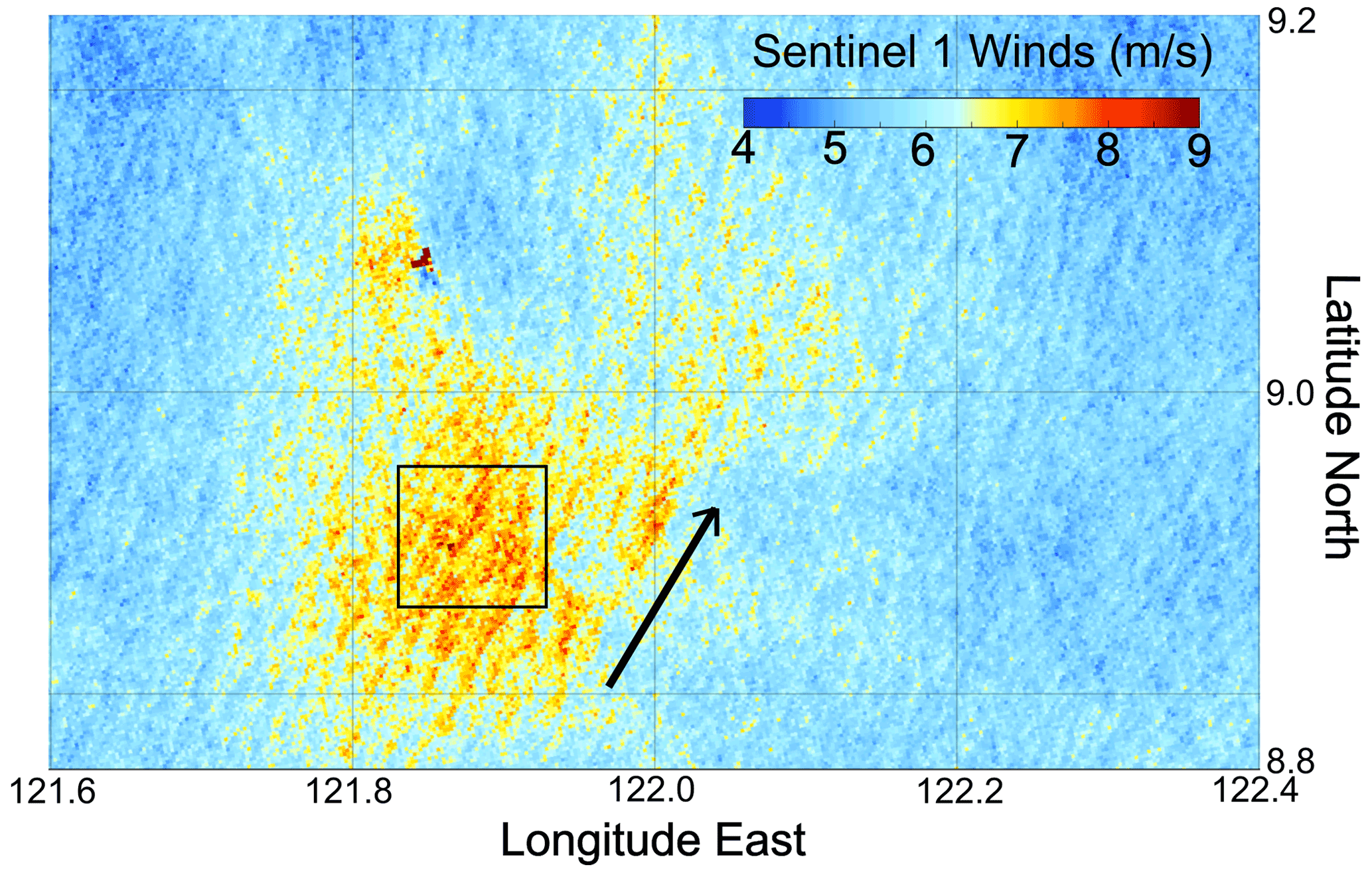
Figure 1 A 250 m resolution image taken from the Sentinel-1 synthetic aperture radar (SAR), post-processed to show surface winds at the Sulu Sea on 1 September 2019. For scale reference, the black box represents a square distance of 11 km in each cardinal direction. The black arrow represents the orientation of the wind direction as given by the ERA5 reanalysis.

To assist in hypothesis evaluation and establishing a predictive range of retrieved SSGFs in field settings, numerical models can be used to help understand volumetric evolution of the MABL from which flux measurements can in turn be simulated (Chen et al., 2018; Eaton and Fessler, 1994; Li et al., 2016; Wei et al., 2018). In this study we examine the effect of turbulence aerosol particle transport through large eddy simulations (LESs) (Moeng, 1984; Sullivan and Patton, 2011) combined with Lagrangian point particles, representing a simple cloud-free marine atmospheric boundary layer with prescribed aerosol particle sources. From this numerical model, uncertainties in simulated aerosol particle flux measurements can be quantified in full 3-D spatiotemporal detail from which flux disaggregation can be achieved in an idealized manner. We study the relation between sampling methodologies, such as stationary and airborne data acquisition; this approach has been previously used to record turbulence statistics in LES-generated settings (Scipión et al., 2008; Wainwright et al., 2015). Here we expand upon previous work with additional features of boundary layer dynamics – turbulent coherent structures and aerosol particle size, as well as their effect on the surface flux of aerosol particles. Finally, we use one-dimensional column models (Kind, 1992; Freire et al., 2016; Nissanka et al., 2018) to estimate net surface emissions and measure their performance against the stationary and airborne data acquisition. Combined, we show the effect of factors which affect the surface flux, including directionality with respect to roll features, aerosol particle size, and height in the boundary layer, and compare how sampling methodologies determine the rate of convergence of the net aerosol flux. These insights aim to assist in both interpretation of field observations of aerosol flux and experimental design.

2 Methodology

2.1 Large eddy simulations with Lagrangian particles

This study uses the National Center for Atmospheric Research (NCAR) large eddy simulation (LES) model (Moeng, 1984) that is combined with Lagrangian particles (NTLP model, see Park et al., 2020; Richter et al., 2021). The Eulerian fields of mass, momentum, and energy are solved using the filtered Navier–Stokes equations with the Boussinesq approximation:

$$\begin{array}{}\text{(1)}& {\displaystyle \frac{\partial {\stackrel{\mathrm{̃}}{u}}_i}{\partial x_i}}=\mathrm{0},\text{(2)}& {\displaystyle }\begin{array}{rl}{\displaystyle \frac{\partial {\stackrel{\mathrm{̃}}{u}}_i}{\partial t}}=& -{\displaystyle \frac{\partial {\stackrel{\mathrm{̃}}{u}}_i{\stackrel{\mathrm{̃}}{u}}_j}{\partial x_j}}-{\displaystyle \frac{\partial {\mathit{\tau }}_{ij}}{\partial x_j}}+{\displaystyle \frac{g{\mathit{\delta }}_{i\mathrm{3}}}{T_{\mathrm{0}}}}\stackrel{\mathrm{̃}}{\mathit{\theta }}-{\displaystyle \frac{\mathrm{1}}{{\mathit{\rho }}_{\mathrm{0}}}}{\displaystyle \frac{\partial \stackrel{\mathrm{̃}}{p}}{\partial x_i}}\\ & +f{\stackrel{\mathrm{̃}}{u}}_{\mathrm{2}}{\mathit{\delta }}_{i\mathrm{1}}+f(U_{\mathrm{g}}-{\stackrel{\mathrm{̃}}{u}}_{\mathrm{1}}){\mathit{\delta }}_{i\mathrm{2}},\end{array}\text{(3)}& {\displaystyle \frac{\partial \stackrel{\mathrm{̃}}{\mathit{\theta }}}{\partial t}}=-\stackrel{\mathrm{̃}}{u_i}{\displaystyle \frac{\partial \stackrel{\mathrm{̃}}{\mathit{\theta }}}{\partial x_i}}-{\displaystyle \frac{\partial {\mathit{\tau }}_{\mathit{\theta }i}}{\partial x_i}},\end{array}$$

where ${\stackrel{\mathrm{̃}}{u}}_i$ is the resolved velocity, $\stackrel{\mathrm{̃}}{\mathit{\theta }}$ is the resolved potential temperature, τ_ij is the subgrid stress, f is the Coriolis parameter, τ_θi is the subgrid turbulent flux of potential temperature, and $\stackrel{\mathrm{̃}}{p}$ is the resolved dynamic pressure containing both hydrostatic and normal forces, which are used to satisfy the divergence-free condition. The Eulerian subgrid-scale turbulent fluxes are parameterized with a prognostic equation that solves for the subgrid-scale turbulent kinetic energy, which is then used to define a mixing length (Deardorff, 1980).

We drive the flow by imposing a constant, unidirectional geostrophic wind U_g. The Eulerian field is assumed periodic in the horizontal (x and y) directions and resolved using a uniform grid in all three directions. At the start of the simulation, an inversion is imposed at the midpoint of the vertical extent (z_inv≈ 510 m), with a radiation condition at the top of the domain (Klemp and Durran, 1983). A pseudo-spectral discretization is used for spatial gradients in the horizontal directions, while a second-order finite-difference scheme is used in the vertical direction. Time integration is done using a third-order Runge–Kutta method, and a divergence-free filtered velocity field is achieved via a fractional step method. The lower boundary condition is prescribed by a rough-wall Monin–Obukhov similarity relation, and the surface is assumed flat with a constant aerodynamic roughness that is representative of the open ocean (z₀ = 0.001 m). Further details of the LES model can be found in Moeng (1984) or Sullivan et al. (1996).

In addition to the integration of the filtered Navier–Stokes equations for boundary layer turbulence, airborne aerosol particles are represented as Lagrangian point particles – a computational method which assumes that the particles are smaller than the smallest resolved scales of the flow (Balachandar and Eaton, 2010) and which allows for straightforward treatment of gravitational settling, inertia, and thermodynamic effects (the latter two are not considered here). As opposed to an Eulerian framework, the Lagrangian approach allows for a natural approach of sampling discrete particles as opposed to a concentration field, given that average concentration and flux profiles remain the same. The Lagrangian point particles are governed by the following equations for their position and velocity.

$$\begin{array}{}\text{(4)}& {\displaystyle }\begin{array}{rl}{x}_{\mathrm{p}}(t+\mathrm{\Delta }t)=& x_{\mathrm{p}}\left(t\right)+v_{\mathrm{p}}\mathrm{\Delta }t+\mathit{\eta }\sqrt{\mathrm{2}\stackrel{\mathrm{‾}}{K}\left(x_{\mathrm{p}}\right)\mathrm{\Delta }t}\\ & +{\displaystyle \frac{\partial \stackrel{\mathrm{‾}}{K}\left(x_{\mathrm{p}}\right)}{\partial z}}\mathrm{\Delta }t\end{array}\text{(5)}& {\displaystyle }{v}_{\mathrm{p}}={\stackrel{\mathrm{̃}}{u}}_{\mathrm{f}}-w_{\mathrm{s}}{\mathit{\delta }}_{i\mathrm{3}}\end{array}$$

Here x_p is the position of particle p, v_p is the particle's velocity, u_f is the resolved fluid velocity interpolated to the particle position using sixth-order Lagrange interpolation, and w_s=τ_pg is the terminal settling velocity of the particle, where τ_p is the Stokes timescale (Wang and Maxey, 1993). In Eq. (4), the final two terms on the right-hand side account for particle transport done by unresolved, subgrid scales. The parameter η is an independent and identically distributed random value from a normal distribution, while $\stackrel{\mathrm{‾}}{K}\left(x_{\mathrm{p}}\right)$ is the average subgrid momentum diffusivity obtained from the LES model interpolated using trilinear interpolating from the surrounding grid points. Overbars refer to averaging in the horizontal directions. The fourth and final term, ${\partial }_z\stackrel{\mathrm{‾}}{K}\left(x_{\mathrm{p}}\right)\mathrm{\Delta }t$, takes into account the vertical transport that is caused by spatial gradients of the mean subgrid diffusivity, which is required to conserve the well-mixed condition that would otherwise be artificially violated (Delay et al., 2005).

Lagrangian–LESs are computationally expensive for sufficient aerosol flux statistics, and some simplifying assumptions need to be made. The simulated Lagrangian sea spray aerosol particles maintain a constant size, meaning that condensation–evaporation or aerosol swell are not considered (Winkler, 1988). Likewise we are not allowing condensation or cloud formation – a topic of ongoing research. We also ignore the momentum and energy exchange between the aerosol particles and the air; that is, we neglect the two-way coupling of droplets within the surface or cloud layers (Peng and Richter, 2019; Mellado, 2017). Lastly, as mentioned above, the LES assumes a flat surface with a prescribed aerodynamic roughness length, although in the open ocean the moving surface waves may play a substantial role in the transport of sea spray aerosol particles in the wave boundary layer (Richter et al., 2019). These simplifications do not impact our primary goal of this study, which is to investigate sampling strategies and statistical convergence of the aerosol source function, and not necessarily the thermodynamic evolution and subsequent turbulence of the fully coupled system. This study is also dependent on the realism of the LES, including the limited domain extent and periodic horizontal boundary conditions; however, we can represent features such as those shown in Fig. 1 and subsequently discuss the importance of fine-scale structure to interpreting field data.

2.2 Simulation configuration

The domain size and number of grid points are held fixed at 10 km × 5 km × 1 km ($x\times y\times z$) and 320 × 320 × 320, respectively. This corresponds to 30 m streamwise × 15 m spanwise horizontal resolution, and roughly 3 m vertical is similar or finer in resolution compared to other convective atmospheric boundary layer studies (Moeng and Sullivan, 1994; Sullivan and Patton, 2011). We define our inversion height z_inv as the location where the planar average of the potential temperature gradient is at its maximum. The inversion height allows us to define a largest eddy timescale as $T_{\text{eddy}}=z_{\text{inv}}/w_{\ast }$, where $w_{\ast }=[\frac{g}{T_{\mathrm{0}}}{Q}_{\ast }{z}_{\text{inv}}{]}^{\mathrm{1}/\mathrm{3}}$ is the convective velocity scale which is a function of the surface heat flux Q_∗, the inversion height z_inv, and a reference temperature T₀ (Deardorff, 1972). The time step is set to 0.5 s with an initial temperature inversion of 0.15 K m⁻¹ beginning at approximately 510 m. The use of such a strong inversion is to limit entrainment and boundary layer growth in order to provide nearly statistically stationary conditions. The minimal growth also maintains a relatively constant (< 5 % difference) value of T_eddy∼ 700 s. The total time of the simulations is 15 000 s, or $t/T_{\text{eddy}}\sim$ 21.5.

We emphasize that our goal is not to literally reproduce real meteorological phenomena, as in Fig. 1, but to obtain a setup that displays a heterogeneous distribution of turbulence and investigate how this affects the transport and subsequent sampling of aerosol particles. This said, general environmental parameters used as boundary conditions of the model do represent the basic features of the wind speed enhancement in Fig. 1. A unidirectional geostrophic wind ($U_{\mathrm{g}}=\mathrm{10}\mathrm{m}{\mathrm{s}}^{-\mathrm{1}}$) and a surface heat flux Q_∗ of 0.02 K m s⁻¹ are applied to force the MABL dynamics (resulting in ∼ 6 m s⁻¹ mean surface wind), representing a typical unstable convective boundary layer corresponding to an air–sea temperature difference of roughly 1.5 K, with a sea surface temperature ${\stackrel{\mathrm{‾}}{\mathit{\theta }}}_{\mathrm{s}}$ of 283 K. We note here that the simulation setup is similar to that of Moeng and Sullivan (1994). The friction velocity u_∗ is around 0.35 m s⁻¹. After running the simulation for 1 h for turbulence spin-up, particles sampled from a monodisperse distribution are generated randomly along an x–y plane at the surface (z = 0 m). Simulations are conducted for two particle sizes with diameters of 10 µm and 50 µm. The 10 µm size is chosen as it largely accounts for the sea salt coarse mode (Reid et al., 2006) and has an appreciably small settling velocity relative to the mixing velocity of turbulence (w_s < 0.3 cm s⁻¹). Likewise, 50 µm is also chosen as the settling velocities become appreciable (w_s∼ 7 cm s⁻¹) and is a common ending size for wing-mounted probes, such as the forward-scattering spectrometer probe (FSSP). Bubble-bursted film or jet droplets can be in this range (Lewis and Schwartz, 2004), as can other sources of “giant” aerosols where production is the most uncertain (Ryder et al., 2019; Jensen and Lee, 2008). The source flux is set to Φ_ss = 0.0002 ${\mathrm{m}}^{-\mathrm{2}}{\mathrm{s}}^{-\mathrm{1}}$, or 10 000 Lagrangian particles over the whole domain per time step for the 10 µm, and it is against this known source flux that the estimates are compared. Sensitivity tests are conducted for 50 000 and 100 0000 Lagrangian particles per second, and although turbulent statistics and concentration profiles remain relatively insensitive to injection rate, the distributions of particle concentration for the simulated instrumentation (explained in Sect. 3.3) are unaltered for the 50 µm sizes at Φ_ss = 50 000 particles per second. If the Lagrangian particles fall below the surface ($x_{\mathrm{p},\mathrm{3}}<\mathrm{0}$), the particle is removed from the simulation, representing dry deposition.

3 Results

3.1 Particle-laden flow characteristics

We first examine the evolution of the aerosol particle concentration in time with the goal of understanding the accuracy of surface flux estimates using common measurement strategies. The normalized vertical concentration profiles are shown in Fig. 2 for 10 and 50 µm diameter particles at multiple times $t_{\text{gen}}/T_{\text{eddy}}$, where ${\stackrel{\mathrm{‾}}{C}}_{\mathrm{r}}$ is the reference concentration, defined to be the concentration at the first grid point (z = 1.6 m); t_gen represents the time since the first generation of particles; and T_eddy is the largest eddy timescale, being around 12 min for the current setup. As expected, the maximum aerosol concentration is located within the surface layer (z≲0.1z_inv) at all times, consistent with results observed in the field (Blanchard et al., 1984; Bian et al., 2019; Schlosser et al., 2020). Above the surface layer, the concentration becomes more uniform, meaning that there is little average variation in height over much of the central portion of the simulation domain. Then, for times $t_{\text{gen}}/T_{\text{eddy}}\gtrsim \mathrm{2}$, the concentration rapidly drops at the inversion, where detrainment is inhibited by the strong inversion and weakened turbulence. In the context of in situ measurements, for $z/z_{\text{inv}}>\mathrm{0.2}$ (or 100 m for a z_inv of 500 m), $\stackrel{\mathrm{‾}}{C}/\stackrel{\mathrm{‾}}{C_{\mathrm{r}}}$ is nearly constant. Yet, 100 m is the minimum altitude at which the NASA P3 and many other research aircraft fly. Under some circumstances, the minimum altitude can be 30 to 50 m, but not under high wind conditions. Therefore, more common in situ ship, tower, or aircraft measurements are at the maximum and minimum values of the concentration profile; observations between the two require special technology such as towed instruments (Yamaguchi et al., 2022) or unmanned aerial vehicle measurements (Kemppinen et al., 2020; Mehta et al., 2021).

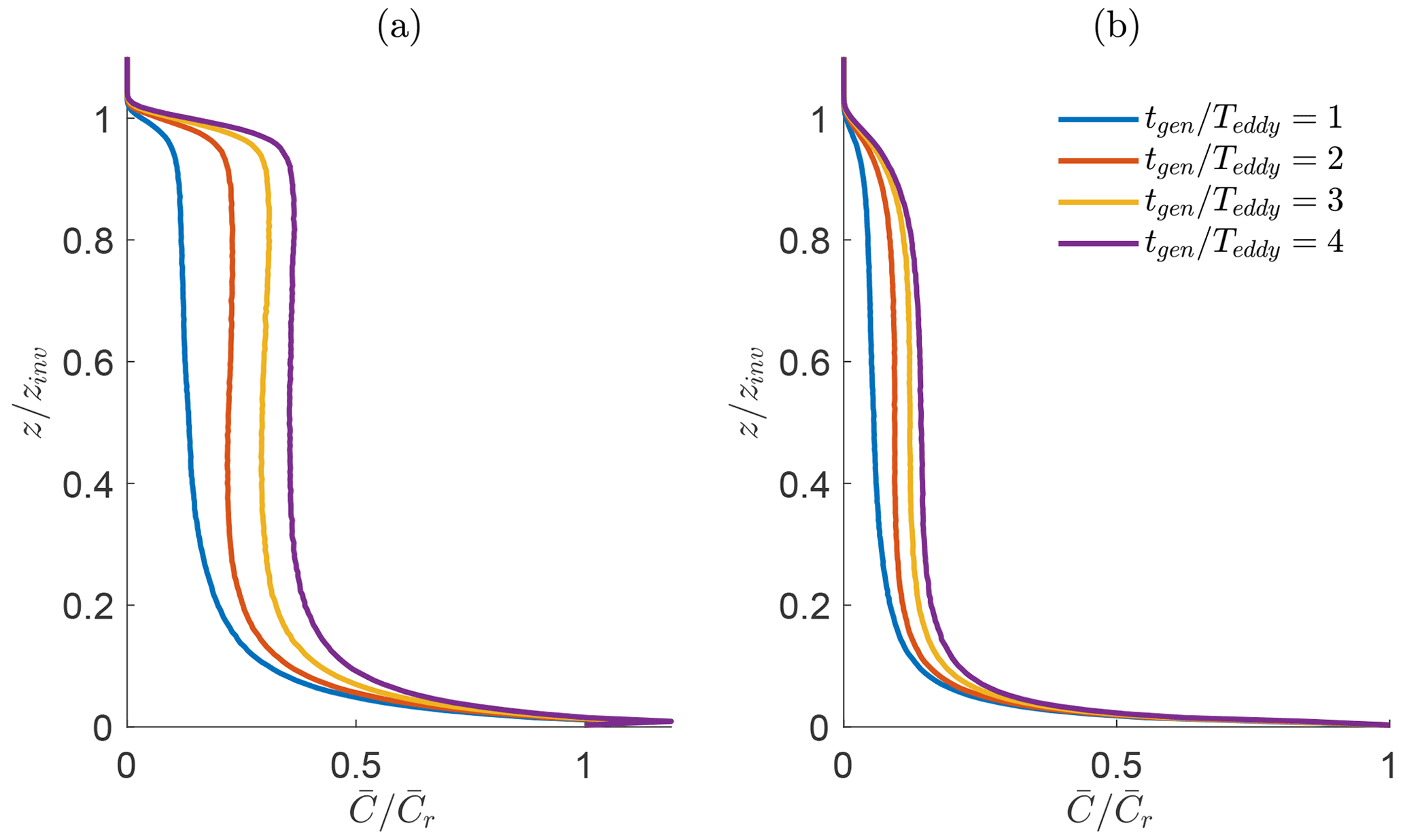
Figure 2 Normalized concentration profiles for (a) 10 µm and (b) 50 µm diameter aerosols at intervals of $t_{\text{gen}}/T_{\text{eddy}}$. The term t_gen is the time since the initiation of surface aerosol generation; T_eddy is the largest eddy timescale, a function of the inversion height and convective velocity scale: it is approximately 12 min.

Although the mass concentration profile is steadily increasing in time, the fluxes (both resolved and subgrid) are expected to approach statistical stationarity soon after particles are introduced. This rapid approach to stationarity of the fluxes and other turbulence statistics, despite the continued growth of aerosol concentration, has been shown in other LES studies (Freire et al., 2016; Nissanka et al., 2018). For simplicity, we remove the effects of initial transients by performing all analysis after $t_{\text{gen}}/T_{\text{eddy}}=\mathrm{2}$. To obtain a baseline quantity to compare against all future turbulent flux measurements, we calculate the net aerosol flux Φ(z) by recording the net number of aerosol particles that have traversed through a plane z = constant at each time step, then divide by the time step and horizontal extent of the domain; these fluxes are calculated at the same Eulerian grid heights (in z) where the flow information is stored. The net aerosol flux is the combination between the turbulent flux against the gravitational settling flux.

Based on the bottom-up diffusion concept for a conservative scalar in a convective planetary boundary layer (Wyngaard and Brost, 1984), we expect the 10 µm aerosol particles (and likewise any smaller particles) to behave largely like passive scalars and therefore exhibit a linear flux with height. This is verified in Fig. 3a, which shows the time-averaged net turbulent flux in blue. The translucent profiles in the background are instantaneous snapshots of the net turbulent flux at the start, middle, and end times of the averaging (only for 10 µm), illustrating that the flux statistics are stationary despite the concentration increasing in time. Although the 50 µm diameter particles (in red) exhibit the same endpoint values, a slight curvature in the flux profile is observed. This is due to the additional presence of a non-negligible settling flux $w_{\mathrm{s}}\stackrel{\mathrm{‾}}{C}$ that modifies the balance for a typical conserved scalar (Nissanka et al., 2018).

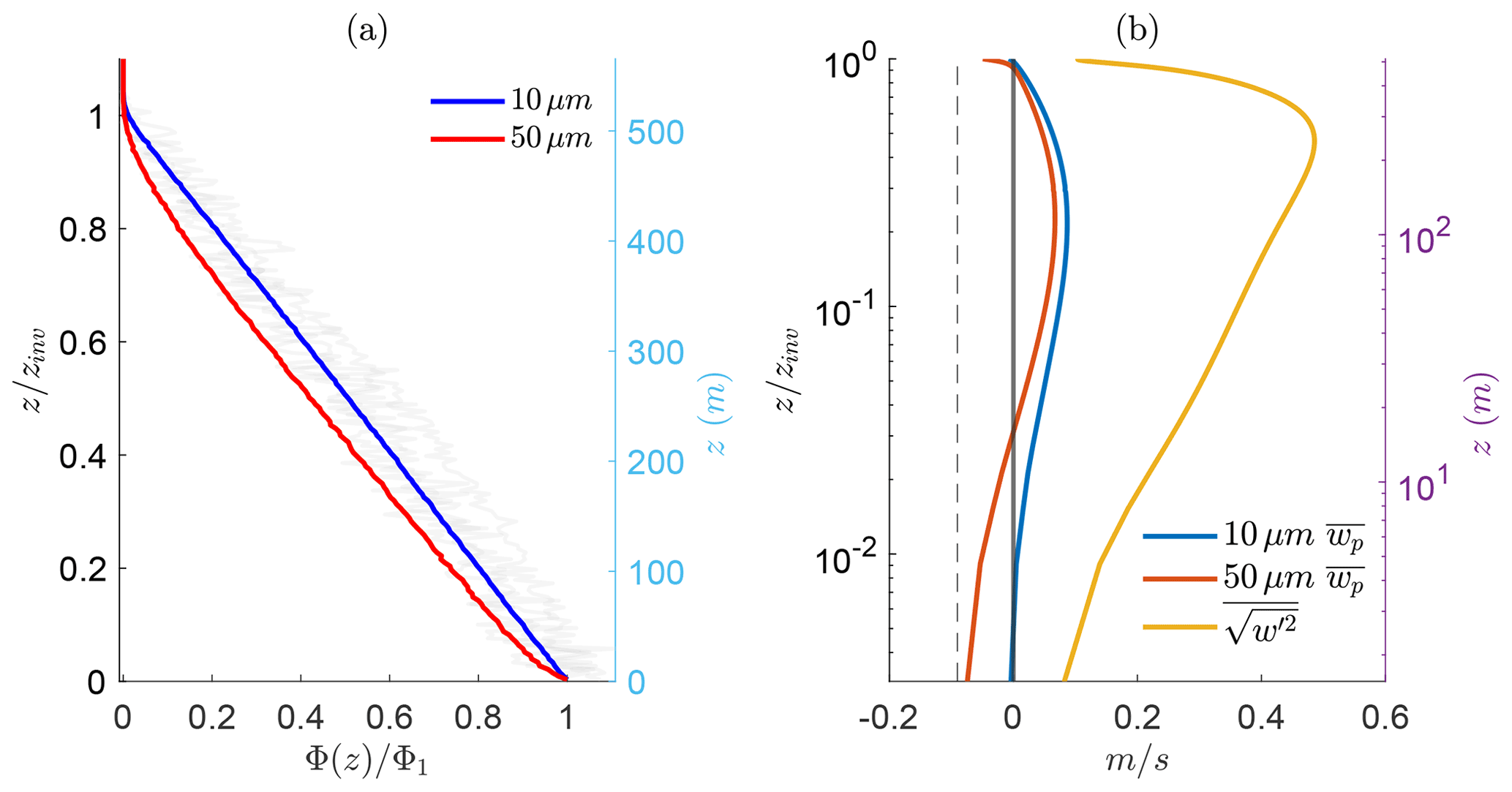
Figure 3 (a) Vertical flux profile for 10 and 50 µm particles normalized by the respective flux at the first grid point (Φ₁). The three faded profiles are the instantaneous net fluxes at the start, middle, and end of the averaging time for 10 µm particles. (b) Comparison of mean particle velocity for both sizes and the standard deviation of the flow vertical velocity at different heights (the left vertical axis is scaled by the inversion height, and the right side is the dimensional height). The dashed line is the gravitational settling velocity for 50 µm particles.

To further investigate the influence of particle size on the flux profiles, we also consider the mean aerosol particle vertical velocity; this can be used as an indicator of gravitational transport over turbulent advection on the aerosol particles. Figure 3b shows the average vertical velocity of the particles at each height ($\stackrel{\mathrm{‾}}{w_{\mathrm{p}}}$) and the fluid vertical velocity variance ($\stackrel{\mathrm{‾}}{\sqrt{w^{\prime \mathrm{2}}}}$). For the 10 µm particles (and smaller), the negligible settling velocity throughout the boundary layer suggests a small deposition rate (thus a long lifetime), for which negative average velocities are reported only up to 1.6 m (the first grid point). On the other hand, heavy 50 µm particles have a negative mean velocity up to 20 m from the surface. This negative mean velocity will lead to an overall deposition of particles this size. The presence of the lower surface and the strong inversion at the top of the boundary layer cause $\stackrel{\mathrm{‾}}{\sqrt{w^{\prime \mathrm{2}}}}$ (in yellow) to be at its weakest in these regions. As a result, the mean vertical velocities of both 10 and 50 µm aerosol particle sizes approach their respective gravitational settling velocities w_s, since this would be the mean velocity in the absence of the surrounding flow (the vertical dashed line indicates the value of w_s for the 50 µm diameter particles).

To provide a more qualitative view of the boundary layer turbulence, Fig. 4 shows instantaneous contours of turbulent vertical velocity in multiple planes cut through the domain. The combined influence of shear- and buoyancy-generated turbulence creates coherent streaks at low levels that are a part of convective roll structures at higher levels; this interaction and the resulting roll structures are well documented in both observations (LeMone, 1973; Grossman, 1982; Weckwerth et al., 1997) and numerical simulations (Moeng and Sullivan, 1994; Khanna and Brasseur, 1998; Salesky and Anderson, 2018).

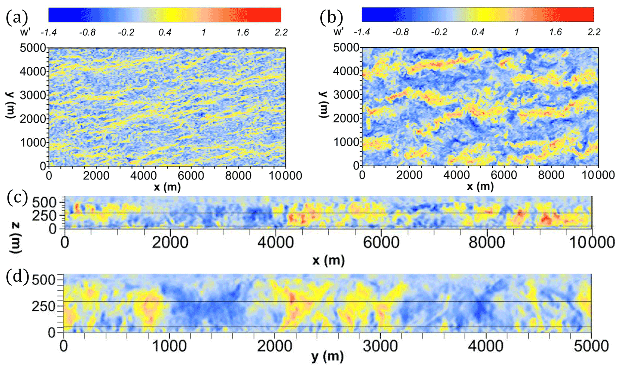
Figure 4 Image of instantaneous vertical velocity contours for an x–y top-down view (a, b), x–z streamwise side view (c), and y–z spanwise side view (d). The x–y top-down views are in panel (a) $z/z_{\text{inv}}=\mathrm{0.083}$ (or 50 m) and in panel (b) $z/z_{\text{inv}}=\mathrm{0.525}$ (or 300 m). x is the streamwise direction of the flow. The solid black lines across (c, d) are the heights of panel (a) and panel (b) plane visualizations.

Considering Fig. 4a, an x–y plane near the upper portion of the surface layer at 50 m ($z/z_{\text{inv}}=\mathrm{0.083}$) exhibits elongated streaks of positive vertical velocities in the streamwise direction. As gravitational settling becomes stronger (e.g., 50 µm), particles require persistent upward velocities to counteract their settling tendency; hence, these streaks are critical for the vertical flux of heavy particles. In Fig. 4b, the assumed “well-mixed” region at z = 300 m ($z/z_{\text{inv}}=\mathrm{0.525}$) exhibits streaks that have grown in spanwise width, with updrafts and downdrafts at their peak values; this height is associated with the highest vertical velocity variance in Fig. 3. From an observational perspective, this horizontal heterogeneity means that if sampling were restricted to only within one of these streaks, then the measured turbulent flux of aerosol would be biased as an overprediction (and vice versa). These boundary layer structures necessitate strategies for achieving full statistical representation. Figure 4c and d show the same velocity contours but for spanwise and streamwise planes (the solid black lines across the x–z and y–z planes are the heights of the x–y plane visualizations in Fig. 4a and b). The surface layer is characterized by a short spatial periodicity of vertical velocity and vice versa in the well-mixed layer.

To further quantify the turbulent coherent structures, we compute their two-point spatial correlations of the vertical velocity in both streamwise and spanwise directions. As noted above, we perform this calculation only after waiting for statistical stationarity, which develops beyond T_eddy∼ 2. These are plotted in Fig. 5 at the same two heights in Fig. 4. Figure 5a is the two-point spatial correlation in the streamwise direction. Near the center of the convective boundary layer (red), the streamwise vertical velocity correlation is strong at multiple inversion heights, while it is significantly weaker in the upper regions of the surface layer (blue). Figure 4b visualizes this effect, whereby instantaneous turbulent structures at 300 m exhibit prominent streamwise coherence compared to 50 m.

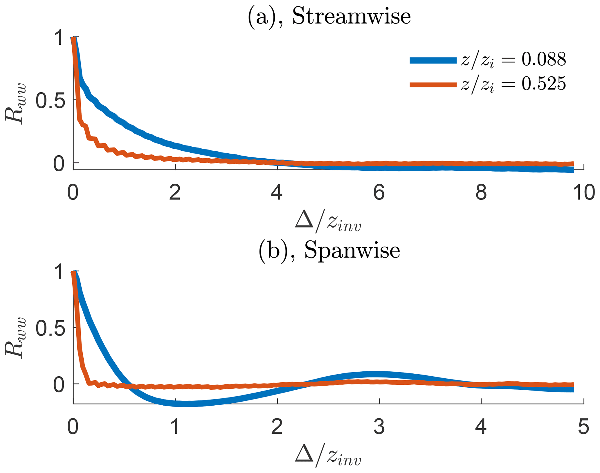
Figure 5 Two-point correlation of vertical velocity variance R_ww in the (a) streamwise and (b) spanwise direction for $z/z_{\text{inv}}=\mathrm{0.088}$ (red) and $z/z_{\text{inv}}=\mathrm{0.525}$ (blue). Δ is the spatial distance dependent on the coordinate direction, nondimensionalized by the inversion height, z_inv.

Figure 5b shows the two-point correlation in the spanwise direction. Near the top of the surface layer (blue), the correlation is again quickly reduced to zero, while the mixed layer exhibits oscillations which are characteristic of alternating streaks of high and low vertical velocity; this can be seen in Fig. 4d where the vertical velocities alternate with distance y. Later, we will show that sampling along these structures causes substantial underprediction or overprediction when estimating a representative aerosol flux.

3.2 Idealized direct flux measurements

Now that the overall LES has been described, we introduce idealized sampling studies to establish a baseline uncertainty of sampled concentration fluxes. To start, we calculate idealized, “true” direct flux measurements from the simulation data as a function of sampling area. Once these direct flux measurements are obtained in height, we will use them to estimate an emission flux and compare it with the known surface flux prescribed in the simulations. That is, to provide an estimate of how representative a limited domain is for a given time span, we systematically decreased the sample domain and compared it to the entire LES to determine the spatial sampling to convergence. While these statistics are not representative of any measurement technology, they are illustrative of the spatial and temporal scales that must be considered when interpreting flux data. Later, these measurements will be used in comparison to the simulated instrumentation and indirect estimate results, tying the analysis to real-world applications and providing a theoretical best-case scenario for computing and evaluating concentration fluxes.

We begin by exploring the effect of limiting the spatial extent of the sampling regions. This is done by directly calculating the net concentration flux in multiple subregions of size 3.1 km², or $\mathrm{1}/\mathrm{16}$ of the horizontal domain. This $\mathrm{1}/\mathrm{16}$ unit area is represented by dark blue in Fig. 6a. We denote this as A_f, where f is the number of these 3.1 km² equal-area rectangles used to create a larger subregion of the total area. In Fig. 6a, the red area, for example, would be denoted as A₄ and uses $\mathrm{1}/\mathrm{4}$ of the total horizontal area to subsample, while the green area would be denoted as A₉. A₁₆ would represent the total area of the domain. While there is no measurement analog for area sampling, this sort of flux disaggregation approach has proved useful in previous numerical studies (Hutjes et al., 2010; Sühring et al., 2019) to conceptualize and compare the subsampled net fluxes ${\mathrm{\Phi }}_{A_{\mathrm{f}}}\left(z\right)$ with the domain-integrated value Φ(z).

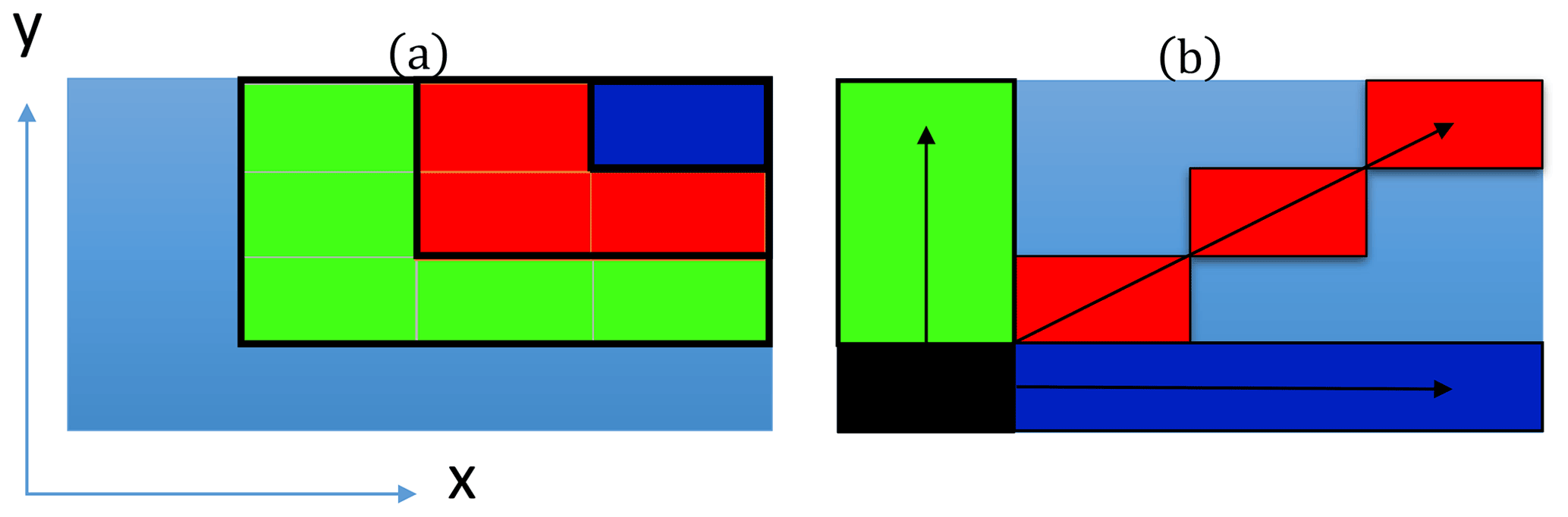
Figure 6 Illustration of the wall-normal plane decomposed into 16 equal-sized rectangles. Panel (a) shows how the sampling region is varied by size; the dark blue rectangle is an example of A₁, the red rectangle is for A₄, and green shows A₉. Panel (b) illustrates the varying directional coverage with a fixed area A₄. The minimum rectangular unit covers 3.1 km², or $\mathrm{1}/\mathrm{16}$ of the horizontal domain area.

We employ these subregions in two ways: first to examine how quickly the subsampled flux ${\mathrm{\Phi }}_{A_{\mathrm{1}}}\left(z\right)$ approaches Φ(z) as a rectangular subsampled area approaches the full domain and second as the same subsampled area A₄ is configured into various directional patterns. The directional-based sampling of the net flux will be susceptible to variability based on the area's alignment with coherent boundary layer structures. With periodic boundary conditions in both horizontal directions and allowing partial overlap of the subregions, there are 16 possible configurations for the rectangular regions of Fig. 6a; the spanwise and streamwise sampling has only four possible configurations, and the diagonal sampling has eight configurations.

We first calculate the flux ${\mathrm{\Phi }}_{A_{\mathrm{1}}}\left(z\right)$, which occurs over each time step of Δt = 0.5 s, after statistical stationarity has been achieved for all 16 regions. These are presented in Fig. 7 as a probability distribution function. Each panel corresponds to a different height, and the sampled particle flux is normalized by the true, domain-wide Φ(z) for the same aerosol particle size. The blue bars represent the probability of 10 µm, and the red represents the 50 µm aerosol particles. In all figures, the expected value is shown by the vertical dashed–dotted line at ${\mathrm{\Phi }}_{A_{\mathrm{1}}}/\mathrm{\Phi }\left(z\right)$ = 1, meaning that the average of the sampled fractional areas converges to Φ(z).

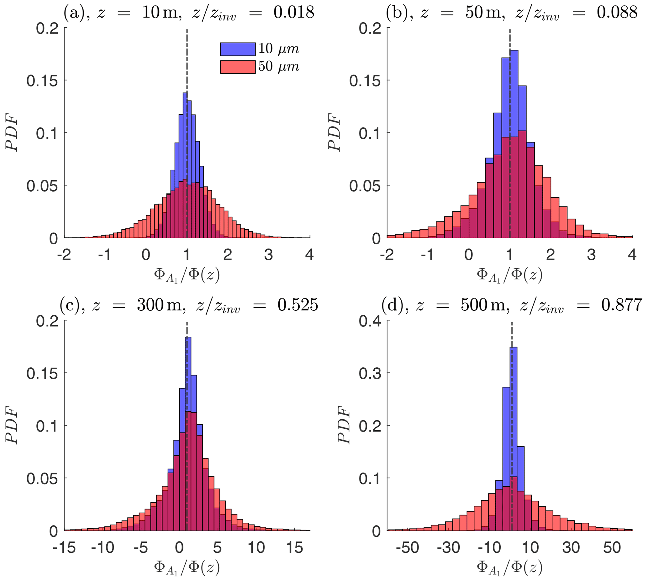
Figure 7 Probability density function of 10 µm (red) and 50 µm (blue) aerosol particle fluxes at z=10 m (a), z=50 m (b), z=300 m (c), and z=500 m (d) for A₁. The pink probabilities signify the overlap of fluxes between the two sizes.

Due to uniform particle sourcing at the surface, Fig. 7a shows that ${\mathrm{\Phi }}_{A_{\mathrm{1}}}$ exhibits the narrowest range of flux for both particle sizes near the bottom of the domain. The heavy 50 µm aerosol particles exhibit a wider variation based on A₁ due to their gravitational settling and their stronger reliance on higher fluid velocities for upward transport. The small 10 µm flux distribution is nearly all a net positive at z = 10 m, but then exhibits negative turbulent fluxes in Fig. 7b, as the turbulent flux broadens for both aerosol particle sizes. The subsequent panels show that aerosol particles that reach higher altitudes will have a larger net flux range for ${\mathrm{\Phi }}_{A_{\mathrm{1}}}$ all the way to the inversion height (note the x-scale change as one considers higher altitudes).

Given this initial analysis, we now quantify in Fig. 8 the range of fluxes recorded at each height for the various subsampled areas (A₁, A₄, and A₉). We take a sample time relevant to field observations (Geever et al., 2005; Norris et al., 2008, 2012): 12 min, or ∼1T_eddy.

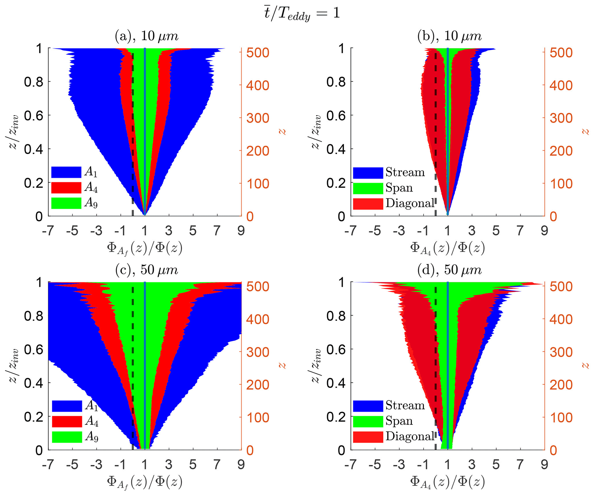
Figure 8 Vertical profiles of flux ranges in sampled (a, b) 10 µm and (c, d) 50 µm aerosol particle fluxes for a time-averaged duration of 1T_eddy. The directional sampling (b, d) is for a sampling area of A₄. Colors from Fig. 6 correspond to those in the current figure. The dashed black line is the zero value reference of net flux, while the solid black line is the reference value for the sampled aerosol particle flux equal to the true, domain-wide LES aerosol particle flux.

For both 10 and 50 µm particles, the ranges between the minimum and maximum net fluxes are shown in Fig. 8. Figure 8a and c are the rectangular configurations, while Fig. 8b and d are for directional-based configurations. The dashed black line in all panels represents the zero flux value (which distinguishes an overall upward or downward net flux), while the blue vertical line represents the mean net flux. The multiple colors in each panel correspond to the subregions of sampling previously described in Fig. 6.

For any rectangular configuration (regardless of size) in Fig. 8a and c, the range in the subsampled net flux increases with height, centered about the mean value of 1. This result can be attributed to the increasing fluid length scales of the turbulent coherent structures as one approaches the center of the mixed layer, as quantitatively shown in Fig. 5 and qualitatively in Fig. 4. The coloring past the zero value line (from a reference point of ${\mathrm{\Phi }}_{A_{\mathrm{f}}}\left(z\right)/\mathrm{\Phi }\left(z\right)=\mathrm{1}$) shows the heights at which a sampled aerosol flux can erroneously report a net downward flux. As expected, sampling from a larger subregion (green being the largest) results in a reduction of the variability in the measured value ${\mathrm{\Phi }}_{A_{\mathrm{f}}}\left(z\right)$.

In Fig. 8b, we quantify the effect of flux sampling based on the directional alignment described in Fig. 6. Again, sampled net fluxes become less representative of Φ(z) with height; either underprediction or overprediction can be sampled from the spread. The streamwise sampling has the largest net flux variability and is attributed to the persistent turbulent structures of high vertical velocity seen in Fig. 4. The diagonal subsampling and streamwise subsampling exhibit similar levels in aerosol net flux variability. Finally, the spanwise sampling (green) in the crosswind direction provides the least variability for the 1T_eddy sampling time considered. These variations in net fluxes, although considering the same subregion A₄, are due to the coherent turbulent structures present in the boundary layer.

Shifting the focus to large 50 µm aerosol particles using the same methodology, Fig. 8c exhibits many of the same features as the 10 µm particles. However, the significant gravitational settling provides a few key differences in the results. The predictive range for both subsampling strategies is nearly doubled compared to the 10 µm counterparts: for example, there is roughly a 100 % increase in predictive range given ${\mathrm{\Phi }}_{A_{\mathrm{1}}}$ at $z/z_{\text{inv}}=\mathrm{0.80}$ and a 300 % increase given the streamwise sampling at $z/z_{\text{inv}}=\mathrm{0.60}$. Since Φ(z) decreases to zero at the top of the boundary layer, this means fewer particles reach that height, resulting in large underpredictions or overpredictions of turbulent flux: this effect is shown in all panels. A net downward flux is more probable when considering the larger range of prediction to the left of the zero reference line. When considering the directional sampling combinations for the 50 µm sizes in Fig. 8d, the same conclusions are made with respect to the 10 µm aerosol particles, namely that the spanwise subsampling provides the fastest convergence towards the true flux, although the flux range increases substantially at the top of the boundary layer.

The disaggregation technique employed here (similar to Sühring et al., 2019, and Hutjes et al., 2010) demonstrates the importance of areal coverage and directional sampling when calculating aerosol mass flux; even in an idealized numerical setting, there is a large range of possible flux values when only sampling a subregion of the turbulent boundary layer. In all cases, this highlights the fact that even if a perfect measurement of flux were to be made at various limited-area heights in the MABL, there is a high likelihood of this measurement not capturing the true surface flux below – in many cases it may even get the sign incorrect. Due to the coherent turbulent structures, the directional sampling causes substantial differences in the net flux, and perhaps intuitively, sampling the domain across the spanwise direction exhibits the fastest convergence towards the true horizontal mean.

While the analysis above discusses the accuracy of sampled fluxes at specific heights under various subsampling strategies, it is often surface aerosol fluxes which are of interest, however, and not necessarily those at some elevated point within the boundary layer. We now use the results above to investigate how this sampling range propagates into inferred surface fluxes.

In the limit of negligible gravitational settling, the aerosol concentration behaves as a conserved scalar and its flux exhibits a linear shape with height; gravity causes this to deviate (see Fig. 3). Regardless of size, however, we fit a linear profile to each profile Φ(z), then extrapolate to the surface to retrieve an inferred surface flux Φ_s,z:

$$\begin{array}{}\text{(6)}& {\displaystyle }m\left(z\right)& {\displaystyle }={\displaystyle \frac{-{\mathrm{\Phi }}_{A_{\mathrm{f}}}\left(z\right)}{z_{\text{inv}}-z}},\text{(7)}& {\displaystyle }{\mathrm{\Phi }}_{\text{s,z}}& {\displaystyle }=-z_{\text{inv}}m\left(z\right),\end{array}$$

where we assume the zero flux at the inversion, Φ(z_inv)=0. We perform this extrapolation from each height by considering the largest overprediction or underprediction of fluxes, similar to the analysis of Fig. 8. Figure 9 shows the inferred effective surface flux Φ_s,z, which is normalized by the time-averaged true surface flux Φ_s at the first grid point. Figure 9a and b represent the 10 µm aerosol particles, and Fig. 9c and d represent the 50 µm aerosol particles. For 10 µm aerosol particles, much of the profile is very similar to Fig. 8a and b, which is to be expected owing to the linearity of the flux Φ(z) of these particles in Fig. 3a. For heavy aerosol particles, however, not only do they have a larger range of ${\mathrm{\Phi }}_{A_{\mathrm{f}}}$ based on subsampling, but the downward bend of the overall turbulent flux (Fig. 3a) also violates the assumption of a linearly decreasing flux profile. This violation causes the curvature in the surface flux profile, with maximum uncertainty at the upper boundary layer heights at $z/z_{\text{inv}}\sim$ 0.7. Thus, for 50 µm aerosol particles, Φ_s,z shows an even wider range of possible values due to the compounding effect of significant settling, leading to a departure of an assumed linear flux profile with height. Note that it is possible to incorporate gravitational settling into the particle flux balance (Nissanka et al., 2018), and this is considered below in Sect. 3.4.

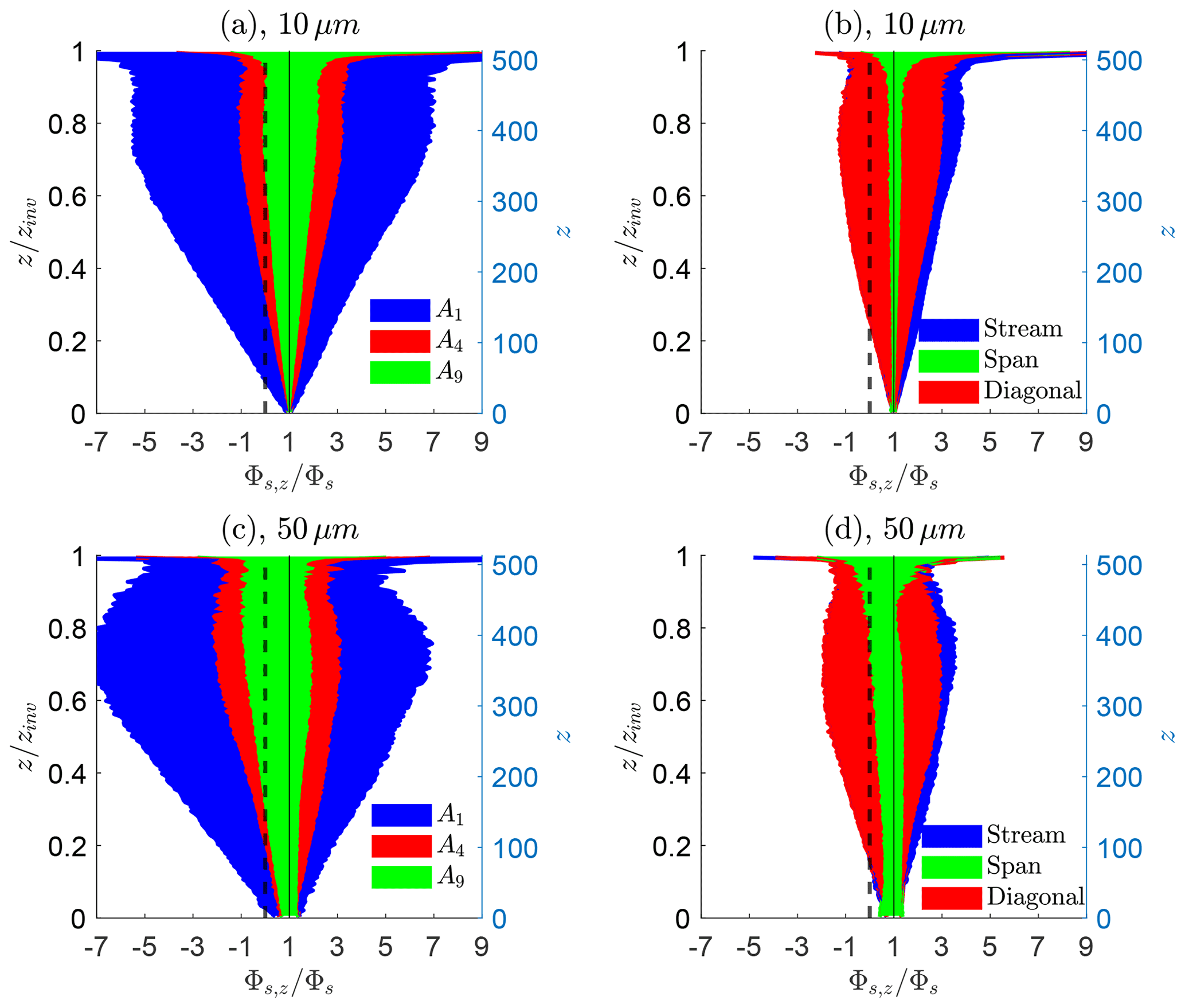
Figure 9 Inferred effective surface fluxes Φ_s,z normalized by the true effective surface flux Φ_s as a function of sampling height for 10 µm (a, b) and 50 µm (c, d) aerosol particles. Elevated fluxes are used to infer surface fluxes via linear extrapolation. The left panels (a, c) illustrate variability due to area coverage, and the right panels (b, d) illustrate directional sampling for the same total area A₄.

Overall, the inferred surface fluxes demonstrate the same level of predictive range as the subsampled net fluxes of Fig. 8. The resulting flux range is amplified when extrapolating to obtain a surface flux – a quantity that is required in regional and global aerosol models. In the next section, we use a similar framework using constraints analogous to field observations.

3.3 Simulated instrumentation

Thus far, we have conducted geometrical subsampling to quantitatively determine the range of estimated net fluxes (both local in height ${\mathrm{\Phi }}_{A_{\mathrm{f}}}\left(z\right)$ and extrapolated to the surface, Φ_s,z) as it is influenced by sampling area. In the interest of better interpreting the observational constraints of field observations, we now turn our attention to simulated instrumentation. In particular, the previous section analyzed the predictive range when the true flux, as computed by the mass of particles crossing a horizontal plane, was calculated exactly. This kind of information, however, is unavailable in practice and only represents a best-case scenario of observations.

Therefore, we now introduce a virtual “probe” to obtain a time series of concentration C(t) and vertical velocity w(t), from which we compute an eddy covariance $\stackrel{\mathrm{‾}}{w^{\prime }{c}^{\prime }}$ within the local LES flow field – a technique more representative of field observations of aerosol fluxes (Norris et al., 2012). Sampling LES-generated fields through simulated instrumentation has been previously performed to evaluate in measurements and identify its potential biases and limitations (Wainwright et al., 2015; Sühring et al., 2019). The results of the eddy covariance for predicting the surface flux Φ_s,z are shown in Fig. 14 in comparison to the other turbulent flux methods.

As we have seen in the previous subsection, sampling across subregions of the flow results in a potentially large spread in estimates of ${\mathrm{\Phi }}_{A_{\mathrm{f}}}\left(z\right)$ and subsequently Φ_s,z due to the coherent turbulent structures and their spatial and temporal correlations. Therefore, it stands to reason that sampling in a manner that captures a representative distribution of the turbulence will result in less uncertainty of aerosol particle flux. To test this hypothesis, an ogive curve can be used to quantify the coherent turbulent structures' effect on the aerosol particle flux. A common technique in field measurements (Desjardins et al., 1989; Friehe, 1991; Norris et al., 2012), an ogive curve Og_wc(f₀) represents a running integral from the highest frequencies to a reference frequency of a co-spectrum:

$$\begin{array}{}\text{(8)}& {\mathrm{Og}}_{\mathrm{wc}}\left(f_{\mathrm{0}}\right)=\underset{\mathrm{\infty }}{\overset{f_{\mathrm{0}}}{\int }}{\mathrm{Co}}_{\mathrm{wc}}\left(f\right)\mathrm{d}f,\end{array}$$

where Co_wc is the co-spectrum of the net aerosol flux $\stackrel{\mathrm{‾}}{w^{\prime }{c}^{\prime }}$. In other words, ogive curves show the convergence rate of a net flux given a defined sampling time. If the reference frequency is set to the lowest possible value based on sampling time, the cumulative integral of the entire spectrum results in the covariance (i.e., the average net flux over that time interval).

To compute an ogive curve, we obtain C(t) and w(t) using two different sampling strategies. First, the virtual probe can be moving (mimicking an aircraft or moving ship) or stationary (say a tower or a stationary ship). Further, each probe has its own sampling volumes and constraints – far too many to simulate here and in fact unnecessary for the point that is being made in this study. For now, consider a probe that has perfect fidelity over a given sampling volume. For each time step (0.5 s), moving probes are translated at a user-defined speed of 50 m s⁻¹ (typical air speeds of a Twin Otter research aircraft) and record both vertical velocity and aerosol concentration over a spherical volume of approximately 1500 m³, or a fraction of 3 × 10⁻⁸ of the domain volume. At the same time, 10 stationary probes are uniformly spaced along the cross-flow direction within the domain, with rows being positioned at z = 50 m and z = 300 m (so 20 stationary probes total). These stationary probes have 9 times the sampling volume compared to the moving probes for statistical sampling convergence. A schematic of the moving and stationary probes in the field of turbulence is presented in Fig. 10b. We perform analysis for sampling durations of 1 T_eddy as done above. A single moving probe is recorded throughout the whole simulation, resulting in six segments of length 1 T_eddy, emulating a total distance of 35 km of aerosol particle sampling.

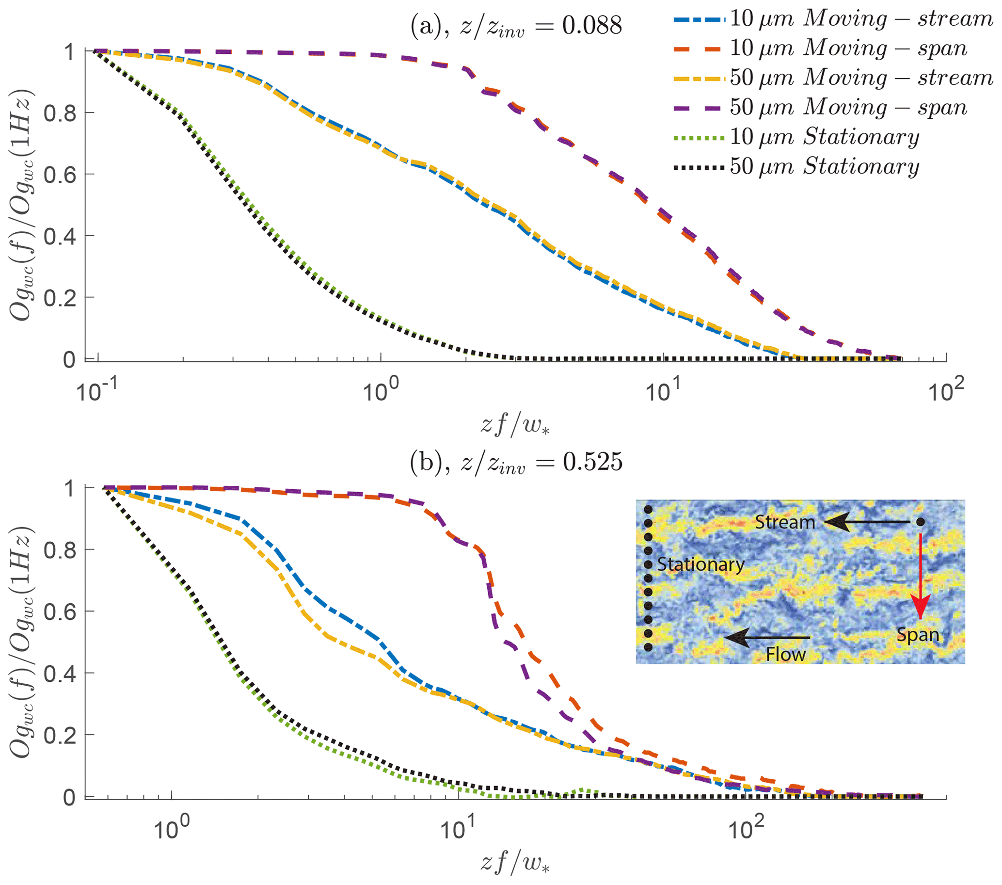
Figure 10 Calculated ogive curves of the net aerosol flux for simulated instrumentation. Moving instrumentation is shown in dashed and dash-dotted lines, while stationary instrumentation is shown in dotted lines at (a) $z/z_{\text{inv}}=\mathrm{0.083}$ and (b) $z/z_{\text{inv}}=\mathrm{0.525}$. Within the moving probe, streamwise (dash-dotted) and spanwise (dash–dash) are presented. Colors are subsequently used to distinguish the aerosol particle size difference. The sampling duration is 1T_eddy. A small schematic figure containing detail of the simulated instrumentation is provided: the left dots represent the spanwise-placed stationary probes, and the upper right dot represents the aircraft sampling in the specified direction.

The net flux convergence through the ogive curves is shown in Fig. 10 for all virtual probes. Consider reading any line in the top panel beginning from the right end of the abscissa to its left end. For any given frequency, the ogive curves accumulate the co-spectrum of the net flux beginning from the highest frequency until the lowest frequency point represents the covariance (normalized to 1). The top panel is from just above the surface layer ($z/z_{\text{inv}}=\mathrm{0.088}$ or z=50 m), and the bottom panel is from within the mixed layer ($z/z_{\text{inv}}=\mathrm{0.525}$ or z=300 m). Legends identify the particle size, moving or stationary, and the direction in which the moving sampling is retrieved. Averages are taken over all 1 T_eddy samples for each probe type and height. Each ogive curve is normalized by its calculated respective covariance value at 2 Hz (${\text{Og}}_{\text{wc},f=\mathrm{2}\mathrm{Hz}}$), while at the highest frequencies the value of Og_wc approaches zero by definition.

For Fig. 10a, there are negligible differences between the net fluxes of different aerosol sizes, as shown by the overlap in each respective virtual instrument. When comparing different instrumentation, however, the convergence rates of the net flux are not the same. For stationary probes, an 80 % net flux convergence requires a lower normalized sampling rate of $zf/w_{\ast }\sim \mathrm{0.2}$, where higher frequencies ($zf/w_{\ast }>\mathrm{20}$) provide a negligible contribution to the total net flux. Since stationary probes (like buoys and flux towers) by definition sample in the streamwise flow direction, they are constrained to the periodicity of the coherent turbulent structures that drift in the spanwise direction over time. Thus, stationary probes require longer sampling times for the traversal of the full range of turbulent structures. Even so, the nonzero slope of the ogive curve at the lowest sampling rate suggests that stationary probes require additional lower frequencies to adequately capture all the scales of the net flux (Norris et al., 2008) (i.e., a sampling duration of 1 T_eddy is not sufficient for a stationary probe). That is, for a tower or stationary ship (often pointed into the wind), turbulent structures align with the flow and are preferentially sampled, thus requiring much longer to achieve convergence with area-average fluxes.

For completeness, we inspect the convergence rate of the net flux with respect to the moving speed by running additional simulations. By varying the moving speed of the probes 100 and 200 m s⁻¹, we consider only the spanwise direction and 10 µm particles at z=300 m for 1 T_eddy. The computed ogive curves (not shown) demonstrate a change in the convergence rate of net flux to shift toward higher normalized frequencies. In other words, probes that traverse faster throughout the boundary layer (given a fixed sampling frequency) require less evaluation time to adequately capture the total net flux of aerosol particles.

As we would expect in the presence of turbulent structures, the ogive behavior is different for streamwise and spanwise moving probes; the leveling-off at low frequencies is indicative of a fully resolved net flux. The same sampling rate of $zf/w_{\ast }\sim \mathrm{20}$ results in a 95 % net flux convergence for spanwise sampling probes. Sampling the coherent turbulent structures across the spanwise direction reduces the required total sampling time, since it captures the overall statistical distribution of the net flux as seen in the previous section. Streamwise sampling achieves around a 60 % net flux convergence for $zf/w_{\ast }\sim \mathrm{20}$. Finally, the nonzero contribution of net flux begins at different sampling frequencies for all simulated instrumentation, with the spanwise sampling beginning at the highest frequencies ($zf/w_{\ast }\sim \mathrm{60}$).

Figure 10b shows the net flux convergence within the mixed layer, where there are a few differences compared to eddy covariance sampling just above the surface layer. First, there are visible, albeit small, discrepancies between particle sizes. Larger particle sizes shift the net flux convergence to lower frequencies (i.e., longer sampling times are required to capture net flux for larger sizes). However, this effect is negligible for stationary probes, for which size again plays a negligible role in the convergence of the net flux compared to the long time required to achieve adequate statistical sampling of the background flow. Second, the start of a nonzero net flux covariance is roughly at the same normalized frequency for both directions of the moving probe, regardless of size.

Overall, the frequencies determining the net flux convergence are unique for all moving and stationary measurements. The streamwise and spanwise sampling of the moving probe requires a shorter sampling time to capture all the necessary frequencies for a net flux convergence. This consideration is critical during the field observation planning of airborne and stationary instrumentation. How these results impact the estimation of Φ_s,z will be discussed below.

3.4 Theoretical flux profile method

Before fast-response sensors were available for eddy covariance measurements, indirect surface flux estimations were made through so-called flux–profile relationships that relate vertical profiles of mean particle concentration to its respective surface flux (Gillette et al., 1972; Gillies and Berkofsky, 2004). These equations are based on the Reynolds-averaged conservation of mass of monodisperse particles under horizontally homogeneous conditions, which (by neglecting molecular diffusivity and applying an eddy diffusivity closure) results in

$$\begin{array}{}\text{(9)}& -K_{\mathrm{C}}{\displaystyle \frac{\mathrm{d}\stackrel{\mathrm{‾}}{C}}{\mathrm{d}z}}-w_{\mathrm{s}}\stackrel{\mathrm{‾}}{C}={\mathrm{\Phi }}_{\mathrm{s}}-\mathit{\beta }z.\end{array}$$

In this equation, $\stackrel{\mathrm{‾}}{C}$ is the horizontal mean particle concentration, K_C is the eddy diffusivity, w_s = $d_{\mathrm{p}}^{\mathrm{2}}{\mathit{\rho }}_{\mathrm{p}}g/\mathrm{18}\mathrm{\mu }$ is the settling velocity (from Stokes' law for a spherical particle, where μ is the dynamic viscosity of air), and $\mathit{\beta }={\mathrm{\Phi }}_{\mathrm{s}}/z_{\text{inv}}$, the surface flux divided by the computed inversion height. Note that for now, in order to introduce and discuss the flux profile method in its ideal form, we use the full horizontally averaged concentration $\stackrel{\mathrm{‾}}{C}\left(z\right)$ known from the LES; however, as above, this true average is not a known quantity in the field. Below, the flux profile method will be subjected to the same types of sampling uncertainties as described in previous sections.

Equation (9) represents the vertical flux budget, combining the turbulent transport (first term) and the gravitational settling (second term on the left-hand side) into a total vertical flux which is assumed to decrease linearly from the effective surface flux Φ_s to zero at z_inv (right-hand side). While this assumption is clearly valid for small particles (see fluxes in Fig. 3a), it may lead to non-negligible error for the larger 50 µm particles.

When representing the surface layer, Eq. (9) can be further simplified by setting β=0, which corresponds to the constant-flux layer assumption (Wyngaard, 2010). In addition, Eq. (9) requires a closure for the eddy diffusivity parameter, which can be obtained by assuming K_C to be proportional to the eddy viscosity parameter (K_m) from the log law of the wall (Davidson, 2004), i.e., $K_{\mathrm{C}}=\mathit{\kappa }z{u}_{\ast }/{\mathrm{Sc}}_{\mathrm{t}}$ (where κ≈ 0.4 is the von Kármán constant and Sc_t = $K_{\mathrm{m}}/K_{\mathrm{C}}$ is the turbulent Schmidt number). Using these assumptions, Chamberlain (1967) and Kind (1992) obtained a general relationship between the effective surface flux and the mean concentration profile of particles, namely

$$\begin{array}{}\text{(10)}& {\displaystyle \frac{\stackrel{\mathrm{‾}}{C}}{{\stackrel{\mathrm{‾}}{C}}_{\mathrm{r}}}}=\left({\displaystyle \frac{{\mathrm{\Phi }}_{\mathrm{s}}}{{\stackrel{\mathrm{‾}}{C}}_{\mathrm{r}}{w}_{\mathrm{s}}}}+\mathrm{1}\right){\left({\displaystyle \frac{z}{z_{\mathrm{r}}}}\right)}^{-w_{\mathrm{s}}{\mathrm{Sc}}_{\mathrm{t}}/\mathit{\kappa }{u}_{\ast }}-\left({\displaystyle \frac{{\mathrm{\Phi }}_{\mathrm{s}}}{{\stackrel{\mathrm{‾}}{C}}_{\mathrm{r}}{w}_{\mathrm{s}}}}\right),\end{array}$$

where ${\stackrel{\mathrm{‾}}{C}}_{\mathrm{r}}$ is the mean concentration at a reference height z_r (note that Sc_t=1 in their original work). Freire et al. (2016) extended this result to include effects of atmospheric stability by using the Monin–Obukhov similarity theory's result $K_{\mathrm{C}}=\mathit{\kappa }z{u}_{\ast }/\mathit{\varphi }\left(\mathit{\zeta }\right){\mathrm{Sc}}_{\mathrm{t}}$, obtaining

$$\begin{array}{}\text{(11)}& \begin{array}{rl}{\displaystyle \frac{\stackrel{\mathrm{‾}}{C}}{{\stackrel{\mathrm{‾}}{C}}_{\mathrm{r}}}}=& \left({\displaystyle \frac{{\mathrm{\Phi }}_{\mathrm{s}}}{{\stackrel{\mathrm{‾}}{C}}_{\mathrm{r}}{w}_{\mathrm{s}}}}+\mathrm{1}\right){\left({\displaystyle \frac{z}{z_{\mathrm{r}}}}\right)}^{-w_{\mathrm{s}}{\mathrm{Sc}}_{\mathrm{t}}/\mathit{\kappa }{u}_{\ast }}\\ & \times \exp \left({\displaystyle \frac{w_{\mathrm{s}}{\mathrm{Sc}}_{\mathrm{t}}}{\mathit{\kappa }{u}_{\ast }}}\mathit{\psi }\left(\mathit{\zeta }\right)\right)-\left({\displaystyle \frac{{\mathrm{\Phi }}_{\mathrm{s}}}{{\stackrel{\mathrm{‾}}{C}}_{\mathrm{r}}{w}_{\mathrm{s}}}}\right),\end{array}\end{array}$$

where $\mathit{\zeta }=z/L$ is the stability parameter ($L=-u_{\ast }^{\mathrm{3}}{\stackrel{\mathrm{‾}}{\mathit{\theta }}}_{\mathrm{s}}/\left(\mathit{\kappa }g\stackrel{\mathrm{‾}}{w^{\prime }{\mathit{\theta }}_{\mathrm{s}}^{\prime }}\right)$ is the Obukhov length), ϕ(ζ) represents stability functions, and the terms in $\mathit{\psi }\left(\mathit{\zeta }\right)\equiv {\int }_{z_{\mathrm{r}}/L}^{z/L}\frac{\mathrm{1}-\mathit{\varphi }\left(x\right)}{x}\mathrm{d}x$ are defined as

$$\begin{array}{}\text{(12)}& \mathit{\psi }\left(\mathit{\zeta }\right)=\left\{\begin{array}{ll}\mathrm{2}\ln \left(\frac{\mathrm{1}+(\mathrm{1}-\mathrm{16}\mathit{\zeta }{)}^{\mathrm{1}/\mathrm{2}}}{\mathrm{1}+(\mathrm{1}-\mathrm{16}{\mathit{\zeta }}_{\mathrm{r}}{)}^{\mathrm{1}/\mathrm{2}}}\right),& \text{if}\mathit{\zeta }<\mathrm{0},\\ -\mathrm{5}\mathit{\zeta }+\mathrm{5}{\mathit{\zeta }}_{\mathrm{r}},& \text{if}\mathit{\zeta }>\mathrm{0},\\ \mathrm{0},& \text{if}\mathit{\zeta }=\mathrm{0}.\end{array}\right.\end{array}$$

Note that due to the assumptions adopted for the eddy diffusivity and β, these equations are expected to be valid in the surface layer only. In addition, Eq. (11) tends to Eq. (10) when stability goes to neutral (ζ→0). From both models, an analytical value of Φ_s can be obtained from two measurements of $\stackrel{\mathrm{‾}}{C}$ at different heights – hence, surface fluxes can be estimated from elevated mean concentrations.

In order to extend these results to the entire ABL, Nissanka et al. (2018) proposed the use of Eq. (9) with $\mathit{\beta }={\mathrm{\Phi }}_{\mathrm{s}}/z_{\text{inv}}$ and

$$\begin{array}{}\text{(13)}& K_{\mathrm{C}}\left(z\right)=\left\{\begin{array}{ll}{\displaystyle \frac{\mathit{\kappa }{u}_{\ast }z}{\mathit{\varphi }\left(\mathit{\zeta }\right){\mathrm{Sc}}_{\mathrm{t}}}},& \text{if}z<z_{\mathrm{b}},\\ a{\displaystyle \frac{\mathit{\kappa }{u}_{\ast }z}{\mathit{\varphi }\left(\mathit{\zeta }\right){\mathrm{Sc}}_{\mathrm{t}}}}{\left(\mathrm{1}-{\displaystyle \frac{z}{z_{\text{inv}}}}\right)}^{\mathrm{2}},& \text{if}z\ge z_{\mathrm{b}},\end{array}\right.\end{array}$$

where z_b is the surface layer height (taken as 0.1 z_inv) and $a=\mathrm{1}/(\mathrm{1}-z_{\mathrm{b}}/z_{\text{inv}}{)}^{\mathrm{2}}$, which creates a continuous transition between the two parts of Eq. (13). Although this model does not provide an analytic solution for Φ_s, it can be used to estimate Φ_s by numerically fitting the model to the data. Note that, for z<z_b, the difference between the Nissanka et al. (2018) and Freire et al. (2016) models comes from the β term only.

As in previous works, a value of Sc_t=1.3 was adopted to account for numerical differences in the diffusivity of particles and momentum in the simulation (Freire et al., 2016; Nissanka et al., 2018). Figure 11a compares the vertical concentration profiles from different theoretical approaches with the simulation result. It is clear that, in the case of non-neutral conditions, the effect of atmospheric stability on the theoretical profile is not negligible, as the Kind (1992) model does not represent the simulation results well. As expected, the Freire et al. (2016) model is similar to the simulation up to z∼0.15 z_inv, whereas the Nissanka et al. (2018) model accounts for the decrease in concentration at z∼z_inv due to the assumption of a linearly decreasing flux profile.

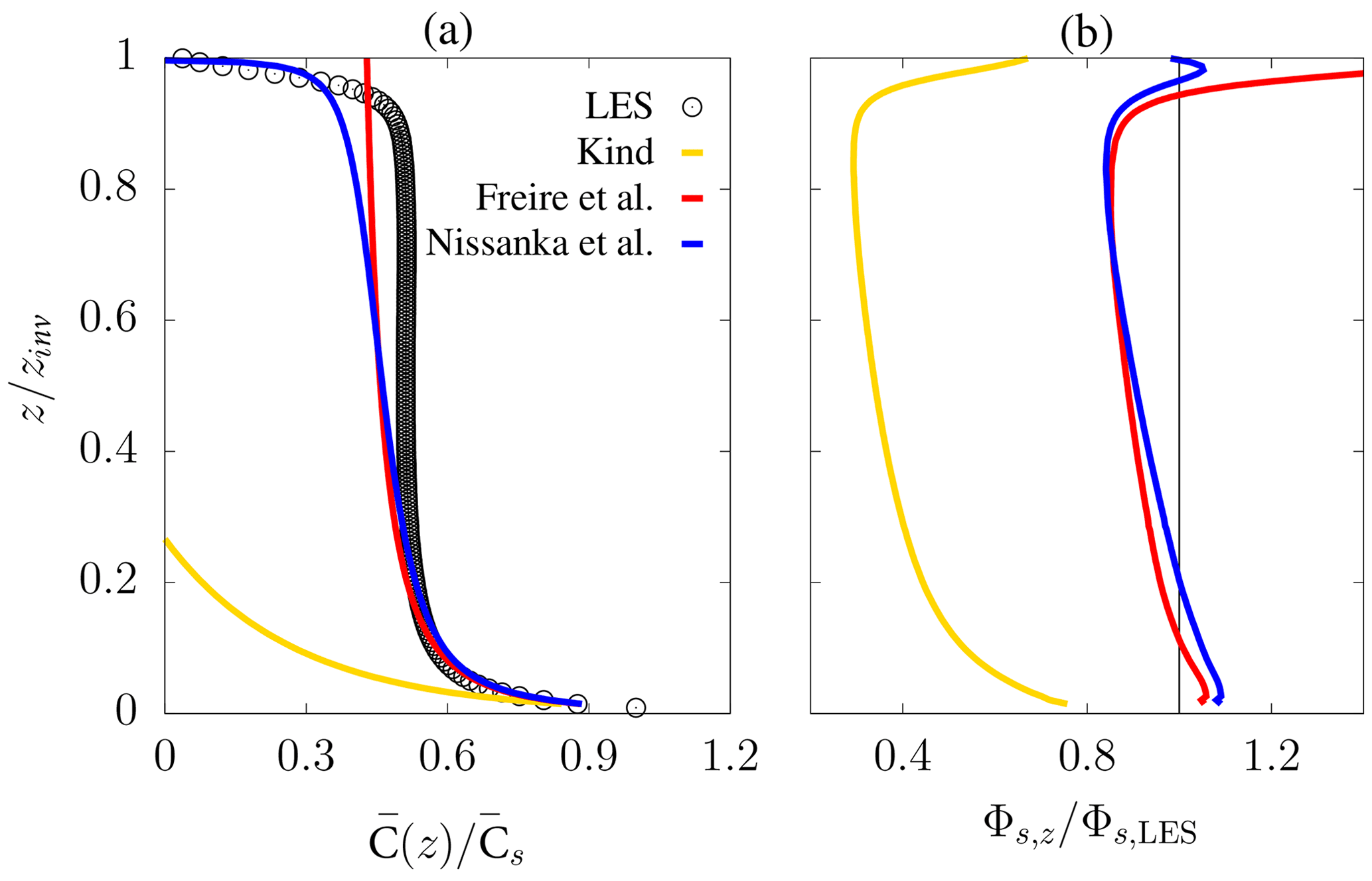
Figure 11 Vertical profiles of the (a) mean particle concentration normalized by its surface value and the (b) estimated surface flux from concentrations at z_r and z (Φ_s,z) normalized by the imposed surface flux in the LES for 10 µm diameter particles. Theoretical profiles from the Kind (1992) model (yellow lines), Freire et al. (2016) model (red lines), and Nissanka et al. (2018) model (blue lines), with LES results in circles. Concentration data were obtained from the time and horizontal average of $t/T_{\text{eddy}}\sim \mathrm{1}$.

By taking the reference concentration ${\stackrel{\mathrm{‾}}{C}}_{\mathrm{r}}$ and a second value at a different height $\stackrel{\mathrm{‾}}{C}\left(z\right)$, it is possible to estimate the effective surface flux Φ_s,z from the theoretical profiles at any height z, as it would be performed in the field if mean concentration values at two different heights were available. The result is presented in Fig. 11b for each height z where a value of $\stackrel{\mathrm{‾}}{C}\left(z\right)$ is available from the LES. From the Kind (1992) model, an underestimation between ∼ 20 % and 70 % is obtained depending on the height of the second concentration value, confirming that the Kind (1992) model is not appropriate for unstable conditions. On the other hand, the Freire et al. (2016) and Nissanka et al. (2018) models provide an error of less than 20 % for heights up to 0.9 z_inv, being similar when compared to each other. While the advantage of using the Freire et al. (2016) model is the analytic solution for Φ_s, the Nissanka et al. (2018) model provides an estimate of Φ_s with less than 10 % error for z∼z_inv. Note that, under neutral conditions, the Kind (1992) and Freire et al. (2016) models provide the exact same result.

We again emphasize that in this flux profile analysis, the calculation of $\stackrel{\mathrm{‾}}{C}$ was taken as a horizontal average over the entire domain. As in the previous section, the convergence of this mean to the true horizontal mean (the theory of Freire et al., 2016, and related flux–profile relationships assume horizontal homogeneity) will be heavily dependent on limited spatial or temporal sampling in much the same way that the fluxes were subject to the influence of the large coherent boundary layer structures. This uncertainty is discussed further in Sect. 4.1, where we use the concentration of the simulated instrumentation for the flux profile method rather than the domain horizontal average.

3.5 Neutral boundary layer

Up to this point we have analyzed the effect of turbulent coherent structures in a typical unstable boundary layer. As atmospheric conditions can widely vary, for completeness we perform additional analysis for a shear-driven, neutrally stratified boundary layer to identify the key differences and similarities. Consideration of a second atmospheric state serves as a helpful foundation for inferring the effects of different stabilities and the resulting sampled net flux. In the case of a neutral boundary layer, the wind shear is solely responsible for the mechanical generation of turbulence (Stull, 1988; Jacob and Anderson, 2017). We provide a briefer synopsis of this configuration, since much of the analysis follows the same patterns as the unstable boundary layer.

The neutral simulations use an identical grid configuration, boundary conditions (both Eulerian and Lagrangian), and geostrophic wind speed (details in Sect. 2.2), but now with $Q_{\ast }=\mathrm{0}$. As a result we define an alternative large eddy timescale which is denoted as $T_{\text{neut}}=z_{\text{inv}}/u_{\ast }$, where u_∗ is the friction velocity recorded at $t_{\text{gen}}/T_{\text{neut}}>\mathrm{2}$. This different large eddy timescale is found to be around 2.5 times longer than T_eddy: around 33 min. Due to the lack of nonlocal, buoyancy-driven transport, the time for turbulence to reach a well-mixed, quasi-steady state takes longer than its unstable counterpart (∼ 1.5 t_gen in Sect. 3.1). As a result, particle generation is initiated at t_gen,neut = 6 T_neut (Φ_ss = 10 000 s⁻¹), and time averaging is done over t_gen,neut + 2 T_neut.

In the neutral boundary layer, the lack of surface heat flux (and thus buoyant convection) results in a different and less organized turbulence structure. Figure 12a shows the contours of vertical velocity at $z/z_{\text{inv}}=\mathrm{0.525}$. The range of the vertical velocities is lower than the unstable boundary layer, leading to less vertical transport of particles throughout the mixed layer and hence the longer time to reach quasi-steady state. Although there are coherent structures visible in the horizontal u and v contours (not shown) qualitatively consistent with previous neutral boundary layer simulations (Jacob and Anderson, 2017), the vertical velocity exhibits a less structured distribution. The vertical velocity correlation lengths in Fig. 12b and c also demonstrate the short spatial coherence of the fluid turbulence relative to the unstable case. Both the streamwise and spanwise correlations drop to zero at the normalized distance $\mathrm{\Delta }/z_{\text{inv}}\sim$ 0.5 or Δ = 300 m, independent of boundary layer height. These differences in the spatial coherence lead to substantial differences in the particles fluxes shown in Fig. 12d, where the temporal and planar-averaged vertical profile of 10 µm (cyan) and 50 µm (green) aerosol particle flux is displayed. The same quantities shown in Fig. 3a are provided as dashed lines for reference. Contrary to the nearly linear profiles of Fig. 3, Φ(z) decreases more quickly from the surface; this effect is again a function of particle diameter. The lack of strongly coherent structures in the neutral boundary layer leads to a more disorganized and thus less efficient upwards transport of particles.

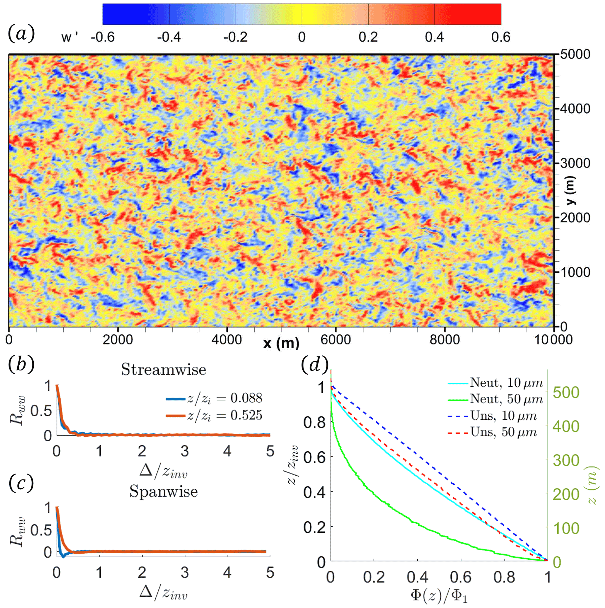
Figure 12 Characteristics of the simulated neutral boundary layer. The top panel (a) is the snapshot vertical velocity field at $z/z_{\text{inv}}=\mathrm{0.525}$. The bottom left panels are the spatial correlation at heights $z/z_{\text{inv}}=\mathrm{0.083}$ and $z/z_{\text{inv}}=\mathrm{0.525}$ for both streamwise (b) and spanwise (c) directions. The bottom right panel (d) is the planar-averaged vertical flux profile for 10 µm and 50 µm diameter aerosol particles. “Neut” stands for the neutral boundary layer configuration, while the dashed references represent the previous unstable boundary layer configuration (abbreviated as Uns).

We perform the same analysis as Sect. 3.2, namely by taking fractional areas A_f as well as directional sampling given A₄ and comparing them to the true Φ(z). Given an averaging time of $\stackrel{\mathrm{‾}}{t}/T_{\text{neut}}=\mathrm{1}$, Fig. 13 shows the results for 10 µm (Fig. 13a and b) and 50 µm (Fig. 13c and d) particles. Again, the left panels show the different A_f for both particle sizes, and the right panels use various directional subsampling.

Figure 13 Vertical profiles of predictive flux ranges for 10 µm (a, b) and 50 µm (c, d) aerosol particle sizes. Panels (a, c) are different subsampling sizes, and panels (b, d) represent directional subsampling given A₄. The panel layout and configurations are identical to Fig. 8.

As before, larger coverage areas provide less variation to Φ(z). For small 10 µm particles (Fig. 13a and b), any subsampling technique applied in this study (with the exception at the top of the inversion height) results in a non-negative net flux result, given the dashed black zero reference. The large oscillation of flux range at high boundary layer levels, especially for larger sizes, is attributed to low particle count due to weak vertical mixing: low counts lead to lacking statistical convergence. In the case of the neutral boundary layer, and in sharp contrast to the unstable boundary layer, Fig. 13b confirms that directional subsampling is inconsequential as a predictor of the net flux, as all three predictions are nearly identical to each other. This is because the lack of coherent boundary layer structure no longer affects the spatial distribution of flux sampling. For the 50 µm particles in Fig. 13c and d, the sampled net flux range is small near the center of the boundary layer when comparing with Fig. 8c and d. The direction again has a minimal difference in accuracy when comparing streamwise, spanwise, or diagonal flow.

Overall, subsampling areas, height in the boundary layer, and aerosol particle size still contribute to the accuracy of representative net fluxes, although the neutral boundary layer estimates of flux experience much less variation. The most significant difference is that directional-based sampling is negligible in predicting Φ(z), as the vertical velocity (associated with its correlation lengths) does not exhibit the same spatial coherence as found in the unstable boundary layer. This difference causes higher aerosol particle concentrations toward the surface layer and lower toward the inversion height. Practically speaking, the results here imply that flux measurements for neutral conditions are representative given a local sampling region: a stark difference to that of the coherent turbulent structures exhibited by an unstable boundary layer.

4 Discussion

Our results conclude that stability, sampling direction, height in the boundary layer, and aerosol particle size are all critical factors to consider when retrieving aerosol fluxes. For unstable conditions, the consideration of convective roll structures is paramount in achieving statistical convergence of net flux measurements. In the context of field observations, impacts of these large coherent structures under commonplace unstable conditions are shown through the unique convergence rates of single-point and moving point measurements (Sect. 3.3). The theoretical profiles in Sect. 3.4 were agnostic to these convective roll structures, but only because they were applied using the true horizontal average over the domain. Finally, a neutral boundary layer state removes the impact of directional sampling, as the vertical velocity roll structures are significantly less pronounced and prove to be inconsequential to aerosol flux measurements. For neutral conditions, measurement challenges and overall biases are greatly reduced. This simple observation from model data under different parameter spaces demonstrates how changes in sampling method can result in integer factor differences in the value of any given flux data point and may thus explain some of the extreme variance in sea salt flux reports in the literature. Nevertheless, in the interest of bridging the gap between all approaches, we compile and summarize the predictive range of Φ_s,z associated with each of the methods.

Summary of prediction ranges

The main purpose of this study is to create a baseline summary of sampled surface flux estimates from different numerical approaches. Doing so bounds the sampled surface flux in predictive range: a critical tool in constricting the order of magnitude variation in surface flux inferences shown in the sea salt literature, thereby informing field observation practices and improving field study design. Due to the large parameter space, we continue to limit our analysis at two heights and two aerosol particle sizes along with both stability cases. We compile the estimated surface flux ranges, including uncertainties from spatial sampling, (1) direct flux measurements, (2) simulated instrumentation which computes an eddy covariance, and (3) the theoretical model.

Before summarizing the prediction ranges of surface fluxes, we briefly mention a couple technical details: one regarding the eddy covariance method and one regarding the theoretical flux profile method. From the simulated instrumentation, we obtain a time series of concentration C(t) and vertical velocity w(t) to compute the net aerosol flux $\stackrel{\mathrm{‾}}{w^{\prime }{c}^{\prime }}$ for 1 T_eddy (recall the discussion of the ogive curves in Sect. 3.3). From this we repeat the procedure described in Sect. 3.2: fit a linear profile to $\stackrel{\mathrm{‾}}{w^{\prime }{c}^{\prime }}$ using a zero flux at the inversion height and extrapolate to the surface to retrieve an inferred surface flux Φ_s,z. We use the largest overprediction or underprediction of fluxes as the basis for the error bars in the following discussion. For the flux profile method, we use the same 1 T_eddy segments of concentration for the two specified heights along with the full horizontal surface concentration (at the first grid point) and apply the theoretical profile of Nissanka et al. (2018) (henceforth denoted as N18) to obtain a surface flux. Again, we use the largest variation of surface flux as the error bars.

The summarized information is presented in Fig. 14, where surface flux estimates are calculated from methods discussed in the previous sections: elevated, idealized flux measurements extrapolated to the surface; eddy covariance using either stationary or moving probes extrapolated to the surface; and the theoretical flux profile method based on the simulated instrumentation aloft combined with the reference surface concentration. Each panel shows both aerosol particle sizes, separated by the slightly transparent center black bar. The first legend item is the idealized direct flux measurement subject to the smallest sampling area. The legend items with EC are based on the numerical instrumentation using eddy covariance. The next legend items are the application of the theoretical profile from N18. Finally, for completeness, the last legend item represents the idealized direct flux measurements under a neutral stability condition for $\stackrel{\mathrm{‾}}{t}/T_{\text{neut}}=\mathrm{1}$. The dashed reference line represents ${\mathrm{\Phi }}_{\text{s,z}}/{\mathrm{\Phi }}_{\mathrm{s}}=\mathrm{1}$, where the estimated surface concentration fluxes match the true LES surface flux.

Figure 14 Summary of the various methods for inferring effective surface fluxes from (a) $z/z_{\text{inv}}=\mathrm{0.088}$ and (b) $z/z_{\text{inv}}=\mathrm{0.525}$. The left side of the abscissa in each plot is for 10 µm diameter aerosol particles, and the right side represents 50 µm sizes. The first legend entry corresponds to the subregion sampling analysis in Sect. 3.2. The second set of legend entries is eddy covariance (EC) and streamwise (as stream), spanwise (as span), and stationary (as stat), corresponding to the simulated instrumentation. The next set of legends corresponds to the Nissanka et al. (2018) model as N18, in which the elevated concentration is constrained by the simulated instrumentation. The last legend item is the surface flux variation from a neutral stability condition for $\stackrel{\mathrm{‾}}{t}/T_{\text{neut}}=\mathrm{1}$. Aside from the last legends, the data are based on an averaging time of 1T_eddy. The dashed reference line represents ${\mathrm{\Phi }}_{\text{s,z}}/{\mathrm{\Phi }}_{\mathrm{s}}=\mathrm{1}$, meaning that the inferred surface flux matches the LES surface flux.

When considering Fig. 14a for the 10 µm particles, the idealized flux measurements at z = 50 m confirm the surface flux variation as we have seen in Sect. 3.2. The eddy covariance results show that the spanwise moving probe provides the closest and most reliable retrieval of Φ_s,z out of any sampling method. In comparison, the large uncertainty shown by the stationary probe is in agreement with the ogive curve discussion in Sect. 3.3: an insufficient sampling time results in a large surface flux range. The N18 model fed with mean concentrations retrieved from simulated instrumentation exhibits a similar uncertainty range, regardless of whether the concentration is measured from a moving or stationary probe. The neutral stratification, subregional sampling shows near-zero variation: this low variation results from sufficiently sampling the turbulent transport of aerosol particles given the relative absence of large, coherent structures spanning the entire depth of the boundary layer.

For the 50 µm particles (right side of the center black bar), all measurements increase in uncertainty, with the stationary probe resulting in the largest overprediction of surface flux, while the N18 model exhibits the greatest negative prediction (or underprediction). From inspection of the concentration time series of the stationary probe for 1 T_eddy (figure not shown), the updrafts carrying aerosol particles cause large positive concentration fluctuations, thereby causing significant ranges of positive surface flux. On the other hand, the N18 results in large negative surface flux prediction (underprediction) due to the violation of the linearly decreasing flux at these large sizes (Fig. 3a). Lastly, the neutral stability of the boundary layer widens in surface flux range for 50 µm particles compared to their 10 µm counterparts, although it remains the most robust of the various estimates.

Near the center of the boundary layer (Fig. 14b), elongated turbulent coherent structures that exhibit the largest spatial correlation can lead to subsampling that is considerably worse in representing the overall surface flux for the unstable condition. Thus, the predictive range for any sampling method is greater when compared to the surface layer flux subsampling. Again, heavier 50 µm particles worsen the predictive range, as the range of estimated surface fluxes increases for all numerical sampling strategies. Given an averaging time of 1 T_eddy, heavier particles and sampling with this height may lead to predictions of a negative surface flux. For the neutral boundary layer, the lack of these turbulent coherent structures causes the variation of inferred surface fluxes to be inconsequential in height (with exception near the inversion), as seen in Fig. 13c and d.

5 Conclusions

This study investigates the fundamental problem of how well a point and/or moving in situ measurement of sea spray aerosol or dust particle can estimate or represent the true surface flux in a turbulent atmospheric boundary layer. The recent data acquisition of the CAMP2Ex field campaign (like Fig. 1) exemplifies the real-world challenges of sampling with regards to the local representativeness of concentration and fluxes obtained. Through the use of large eddy simulations combined with Lagrangian point particles, we simulate a configuration of coherent turbulent structures that analogously demonstrates the heterogeneous nature of aerosol particle transport.

These numerical simulations, which provide full 3-D spatiotemporal detail, are then used to measure aerosol particle surface fluxes through three approaches. The first approach was through a direct method whereby particles are counted crossing a horizontal boundary using multiple configurations of subregions to compare their net aerosol flux with the domain-integrated value. This approach results in a net flux range that is found to be sensitive to multiple parameters: aerosol particle size, spatial sampling strategy, and height in the boundary layer. Indeed, the spatial correlation of the roll structures is dependent on height (Fig. 4), causing differences in the predictive range of net aerosol flux. Gravitational settling based on size competes against turbulent transport that would otherwise lead to tracer-like behavior of aerosol particles (Fig. 3b). These aerosol fluxes were then used to estimate a surface flux which could be compared to the known emission flux, since surface fluxes are required in regional and global aerosol models for forecasting. The surface flux variability was found to be nearly monotonic in height (Fig. 9), with a nearly 50 % increase when considering 50 µm sizes from the small tracer particles. The directional subsampling (given a sampling subregion A₄) also supports this and offers the lowest predictive range in the spanwise subsampling direction.

Using simulated instrumentation similar to field practices as the second approach, moving airborne and stationary probes were used to sample the simulated LES fields in computing an eddy covariance. These were also presented in the form of ogive curves (Fig. 10), which suggest that the manner of observation (whether moving or stationary), directionality (streamwise or spanwise sampling for the moving probe), and aerosol particle size determine the important frequencies of the aerosol flux: our results suggest that, given a sampling duration of 1T_eddy, stationary probes require additional lower frequencies (meaning a longer sampling time) to adequately capture all of the scales of the turbulent flux. As expected, sampling in the spanwise direction provides the least amount of time required in sampling the true flux. The eddy covariance technique was then also used to estimate a surface flux. The results suggest that the method of aerosol particle sampling results in unique surface flux variability due to coherent roll structures with the marine atmospheric boundary layer. The sampling method for surface flux variability can result in integer factor differences in the value of any given flux data point and may thus explain some of the extreme variance in sea salt flux reports in the literature, especially for large particle sizes.

The third approach uses the flux profile method for surface flux extraction. This approach is used in two ways: one procedure, meant to provide a theoretical best-case prediction, uses horizontally averaged elevated concentrations to compare the accuracy of the theoretical flux profiles in calculating surface flux between Kind (1992), Freire et al. (2016), and Nissanka et al. (2018). The N18 model provides a small underestimation of less than 10 % for 10 µm aerosol particle sizes. The second procedure applies the N18 model using concentration segments provided by the simulated instrumentation for streamwise or spanwise moving and stationary probes. While the N18 model records small surface flux variability for 10 µm particles, substantial variability is found for 50 µm particles.

Although the direct flux approach is purely numerical, the approach suggests that potentially large uncertainty in measurements extrapolating the surface flux is inevitable, even with perfect sampling. Again, this result is attributed to the convective roll features. This attribution is further validated through the converse, in which the neutral boundary layer has a significantly lower range of surface flux variability based on lack of vertical coherence: the flow field demonstrates a more local distribution of turbulent transport. In the context of more realistic point or moving sampling strategies in the atmospheric boundary layer, these results suggest that in an unstable boundary layer, the recommended frequency and duration of sampling measurements are constrained to the manner of the observation.

We conclude that, given all the assumptions and constraints initially provided in the study (such as mesoscale and synoptic-scale negligence and a realistically based sampling duration), there is surface flux variability due to coherent turbulent structures that affect sampling across boundary layer height and aerosol particle size. To better constrain this flux variability, the heterogeneous patterns of turbulent flow due to the convective roll features must be taken into consideration. Although the focus of this study emphasizes sea spray aerosol particles over the open ocean, this analysis can in principle be applied to dust or any other kind of particle that is transported from the surface aloft. As this is the first of several studies to better interpret field data, this study acts as a foundation in bridging the gap between numerical simulations and in situ acquisition of aerosol particle transport information.