Volcanic cloud detection using Sentinel-3 satellite data by means of neural networks: the Raikoke 2019 eruption test case

Accurate automatic volcanic cloud detection by means of satellite data is a challenging task and is of great concern for both the scientific community and aviation stakeholders due to well-known issues generated by strong eruption events in relation to aviation safety and health impacts. In this context, machine learning techniques applied to satellite data acquired from recent spaceborne sensors have shown promising results in the last few years.

This work focuses on the application of a neural-network-based model to Sentinel-3 SLSTR (Sea and Land Surface Temperature Radiometer) daytime products in order to detect volcanic ash plumes generated by the 2019 Raikoke eruption. A classification of meteorological clouds and of other surfaces comprising the scene is also carried out. The neural network has been trained with MODIS (Moderate Resolution Imaging Spectroradiometer) daytime imagery collected during the 2010 Eyjafjallajökull eruption. The similar acquisition channels of SLSTR and MODIS sensors and the comparable latitudes of the eruptions permit an extension of the approach to SLSTR, thereby overcoming the lack in Sentinel-3 products collected in previous mid- to high-latitude eruptions. The results show that the neural network model is able to detect volcanic ash with good accuracy if compared to RGB visual inspection and BTD (brightness temperature difference) procedures. Moreover, the comparison between the ash cloud obtained by the neural network (NN) and a plume mask manually generated for the specific SLSTR images considered shows significant agreement, with an F-measure of around 0.7. Thus, the proposed approach allows for an automatic image classification during eruption events, and it is also considerably faster than time-consuming manual algorithms. Furthermore, the whole image classification indicates the overall reliability of the algorithm, particularly for recognition and discrimination between volcanic clouds and other objects.

1 Introduction

From the start of an eruptive event, volcanic emissions are composed of a broad distribution of ash particles, from very fine ash (particle diameters, d<30 µm) increasing in size to tephra (airborne pyroclastic material) with diameters in the range of 2–64 mm. Larger fragments, which fall out quickly, are also generated; these and ash with d>30 µm are not considered in this paper. The gaseous part of an eruptive event is made up mainly of water vapor (H₂O), carbon dioxide (CO₂), and sulfur dioxide (SO₂) gases (Oppenheimer et al., 2011; Shinohara, 2008); a liquid part consisting of sulfate aerosols is also present. Depending on the eruptive intensity, the volcanic cloud can reach different altitudes in the atmosphere, thus affecting the environment (Craig et al., 2016; Delmelle et al., 2002), climate (Bourassa et al., 2012; Haywood and Boucher, 2000; Solomon et al., 2011), human health (Delmelle et al., 2002; Horwell et al., 2013; Horwell and Baxter, 2006; Mather et al., 2003), and aircraft safety (Casadevall, 1994).

The detection procedure consists of identifying the presence of certain species in the atmosphere and distinguishing them from other species. Thus, volcanic ash detection is related to the determination of the areas (pixels in an image) which are affected by the presence of these particles. The first evidence regarding the possibility of detecting volcanic clouds by means of remote sensing data arose in the eighties (Prata, 1989a, b). The method used for the detection of volcanic ash particles relies on the ability to discriminate volcanic clouds from meteorological ice and liquid water clouds by exploiting the different spectral absorptions in the thermal infrared (TIR) spectral range (7–14 µm). In this interval, the absorption of ash particles with radiuses between 0.5 and 15 µm at a wavelength of 11 µm is larger than the absorption of ash particles at 12 µm. The opposite happens for meteorological clouds, which absorb more significantly at longer TIR wavelengths. Therefore, the brightness temperature difference (BTD) – i.e., the difference between the brightness temperatures (BTs) at 11 and 12 µm – turns out to be negative ($\mathrm{\Delta }{T}_{\mathrm{11}-\mathrm{12}\mathrm{\mu }\mathrm{m}}<\mathrm{0}$ ^∘C) for regions affected by volcanic clouds and positive ($\mathrm{\Delta }{T}_{\mathrm{11}-\mathrm{12}\mathrm{\mu }\mathrm{m}}>\mathrm{0}$ ^∘C) for regions affected by meteorological clouds.

The BTD approach is the most used method for volcanic cloud identification. It is effective and simple to apply, even if it can, in some cases, lead to false alarms, e.g., over clear surfaces during the night, on soils containing large amounts of quartz (such as deserts), on very cold or icy surfaces, or in the presence of high water vapor content (Prata et al., 2001). As already mentioned, the discrimination between volcanic and meteorological clouds is a challenging task, since the region of the overlap of the two shows mixed behaviors that are not easily recognizable. In these mixed scenarios, the BTD can be negative not only for volcanic clouds but also for meteorological clouds; thus, some false positive results may occur, as in the case of high meteorological clouds. False negative results may arise in the case of high atmospheric water vapor content: the water vapor contribution can hide and cancel out the effects of ash particles on the BTD, and then the ashy pixels cannot be revealed. In these cases, a correction procedure can be applied (Corradini et al., 2008, 2009; Prata and Grant, 2001). In addition to the described procedures, other algorithms have been developed (Francis et al., 2012; Pavolonis, 2010; Pavolonis and Sieglaff, 2012; Clarisse and Prata, 2016).

For these reasons, it seems appropriate to use advanced classification schemes to address the task of ash detection – e.g., using approaches which make use of machine learning techniques, avoiding the need to find for each product the best BTD threshold for manually creating the volcanic cloud mask, which can be a time-consuming process.

For aerosol and meteorological cloud detection, a neural network (NN)-based algorithm (Atkinson and Tatnall, 1997; Bishop, 1994; Di Noia and Hasekamp, 2018) allows for the solution of a classification problem. Starting from inputs containing spectral radiance values acquired in a specific wavelength band, the model generates a prediction as output by assigning to each pixel of the original image a predefined class. In previous research, neural networks have already shown significant effectiveness in terms of atmospheric parameter extraction (Gardner and Dorling, 1998), specifically for volcanic eruption scenarios (Gray and Bennartz, 2015; Picchiani et al., 2011, 2014; Piscini et al., 2014). A strong advantage of using an NN-based approach for volcanic cloud detection is that, once the model is trained on a statistically representative selection of test cases, new imagery acquired over new eruptions can be accurately (depending on the training phase) classified in near-real time, allowing for significant advantages in critical situations and in emergency management.

In this work, we developed an NN-based algorithm for volcanic cloud detection using Sentinel-3 SLSTR (Sea and Land Surface Temperature Radiometer) daytime data with a model trained on MODIS (Moderate Resolution Imaging Spectroradiometer) daytime images. This is possible due to the two sensors having similar spectral bands, and it represents an advantage, as there is currently limited use of SLSTR products for eruptive events. The use of MODIS as a proxy for SLSTR was already successfully tested in a previous work investigating the complex challenge of distinguishing between ice and meteorological clouds (also containing ice) using neural networks on SLSTR data (Picchiani et al., 2018). As a test case, the Raikoke 2019 eruption has been considered in this work.

2 Case study: the Raikoke 2019 eruption

The Raikoke volcano is located in the Kuril Island chain, near the Kamchatka Peninsula in Russia (48.3^∘ N, 153.2^∘ E). On 21 June 2019, at about 18:00 UTC, Raikoke started erupting and continued erupting until about 03:00 UTC on 22 June 2019. During this period, Raikoke released large amounts of ash and SO₂ into the stratosphere.

Figure 1 shows a time series of 11 µm brightness temperatures (BTs) determined by the Himawari-8 AHI (Advanced Himawari Imager) sensor at 10 min intervals for the first 18 h of the eruption. With the purpose of searching for high (cold), vertically ascending clouds resulting from an eruption and not of meteorological origin, discrete eruptions were identified by comparing AHI BTs near the vent with those some distance upwind from the vent. The Himawari-8 time series shows a sequence of eruptions (12 in all) and a sustained period of activity between 22:40 of 21 June and 02:10 of 22 June, when the majority of ash and gas was emitted. The estimated time of an eruption event was determined by examining animated images, and consequently, the times of the eruptions shown do not always coincide with the coldest cloud top. It is estimated from the AHI data that the June 2019 Raikoke eruption produced approximately 0.4–1.8 Tg of ash (Bruckert et al., 2022; Muser et al., 2020; Prata et al., 2022) and 1–2 Tg of SO₂ (Bruckert et al., 2022; Gorkavyi et al., 2021). The amount of water vapor emitted is unknown but would have been considerable, as is common in most volcanic eruptions (Glaze et al., 1997; McKee et al., 2021; Millán et al., 2022; Murcray et al., 1981; Xu et al., 2022). These emissions would have led to copious amounts of water and ice clouds being produced (McKee et al., 2021; Rose et al., 1995), making the composition of the transported clouds both complex and changing with time.

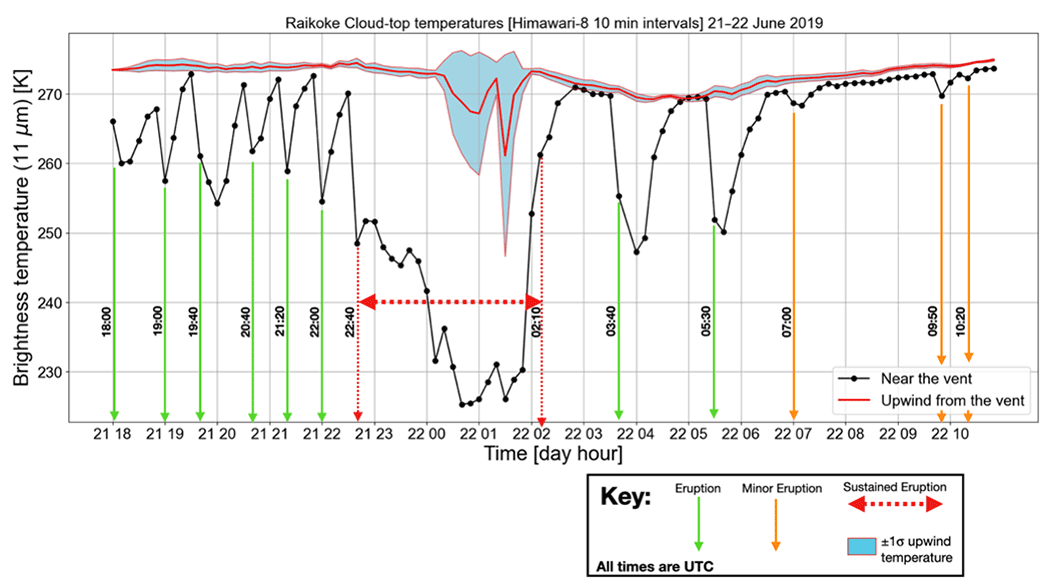
Figure 1 Time series of the eruptions from Raikoke during the first 18 h of activity. The times of the eruptions were estimated from the imagery and do not always coincide with the coldest cloud tops. The black line is the average within a box bounded by the latitude and longitude coordinates: 153.25–153.35^∘ E, 48.32–48.42^∘ N. The red line (upwind) is the average within a box bounded by: 153.10–153.20^∘ E, 48.32–48.42^∘ N.

3 Instruments

In this section, the specifications of the instruments that provide the products used to conduct the research are described. The MODIS sensor on board Terra and Aqua satellites has been used to set up the training dataset of an NN-based model. The SLSTR sensor on board Sentinel-3A and Sentinel-3B satellites has been used for the application of the aforementioned model.

3.1 MODIS instrument

MODIS aboard NASA Terra and Aqua polar orbit satellites is a multispectral instrument, with 36 channels from VIS to TIR, ranging from 0.4 to 14.4 µm, and with spatial resolutions of 0.25 km for bands 1–2, 0.5 km for bands 3–7, and 1 km for bands 8–36. The two spacecraft fly at a 705 km altitude in a sun-synchronous orbit, with a revisit cycle of about 1 or 2 d. The Terra spacecraft was launched in 1999, and its equatorial crossing time is 10:30 UTC (descending node), while Aqua was launched in 2002, and its equatorial crossing time is 13:30 UTC (ascending node).

In our work, we used several MODIS products from both Terra and Aqua platforms: Level-1A geolocation fields (MOD/MYD03) (see Nishihama et al., 1997, for details); Level-1B calibrated radiances (MOD/MYD021KM) (see Toller et al., 2017, for details), which has been used to generate the brightness temperatures (BTs); Level-2 surface reflectance (MOD/MYD09) (see Vermote and Vermeulen, 1999, for details); and Level-2 cloud product (MOD/MYD06_L2) (see Menzel et al., 2015, for details).

3.2 SLSTR instrument

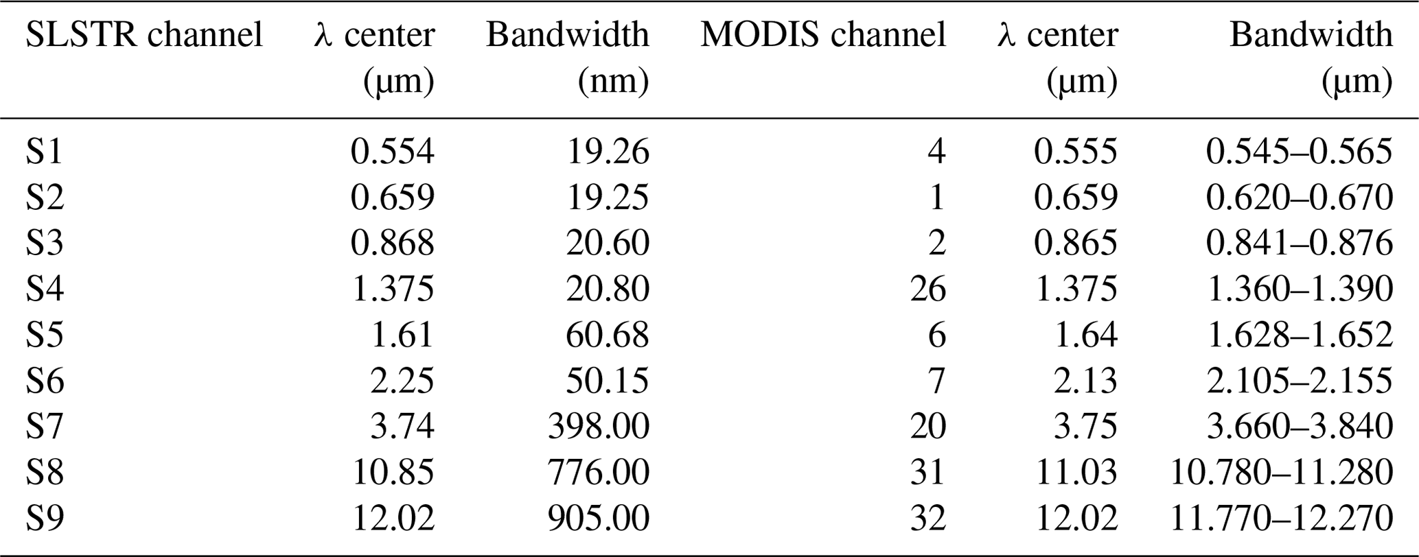
The Sea and Land Surface Temperature Radiometer (SLSTR) is one of the instruments on board the Sentinel-3A (S3A) and Sentinel-3B (S3B) polar satellites launched in 2016 and 2018, respectively. Sentinel-3 is designed for a sun-synchronous orbit at 814.5 km of altitude, with a local equatorial crossing time of 10:00 UTC. The revisit time is 0.9 d at the Equator for a two-operational spacecraft configuration. The orbits of the two satellites are equal, but S3B flies ±140^∘ out of phase with S3A. The basic SLSTR technique is inherited from the technique used by the series of conical scanning radiometers starting with the ATSR. The instrument includes the set of channels used by ATSR-2 and AATSR (0.555–0.865 µm for VIS channels, 1.61 µm for SWIR channel, 3.74–12 µm for MWIR/TIR channels), ensuring continuity of data, together with two new channels at wavelengths of 1.375 and 2.25 µm in support of cloud clearing for surface temperature retrieval. The SLSTR radiometer measures a nadir and an along-track scan, each of which also intersects the calibration black bodies and the visible calibration unit once per cycle (two successive scans). Each scan measures two along-track pixels of 1 km (4 or 8 pixels at 0.5 km resolution for VIS–NIR channels and SWIR channels, respectively) simultaneously. This configuration increases the swath width in both views and also provides a 0.5 km resolution in the solar channels. Our procedure makes use of the SLSTR Level-1 TOA (top-of-atmosphere) radiances and brightness temperature product from both platform S3A and S3B – see Cox et al. (2021) for details of SLSTR Level-1 product.

4 Methodology

In this section, the adopted methodology is described. The procedure has been developed in a MATLAB environment, and the source codes are available upon request, as explained in the Code Availability section. In particular, the MATLAB deep learning toolbox has been used to implement the NN.

A multilayer perceptron neural network (MLP NN) was trained with MODIS daytime data, and then it was applied to Sentinel-3 SLSTR daytime products in order to discriminate ashy pixels from others, following the scheme reported in Fig. 2.

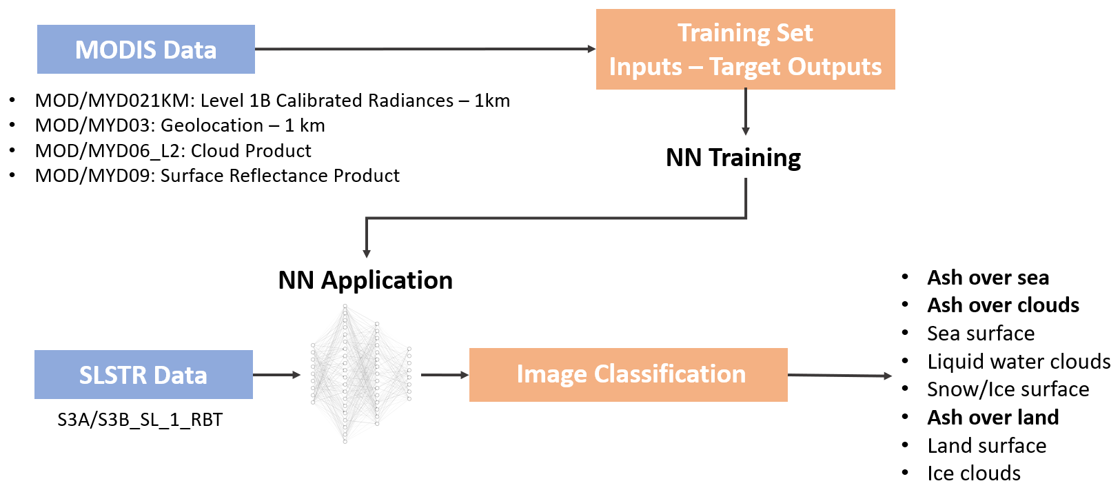
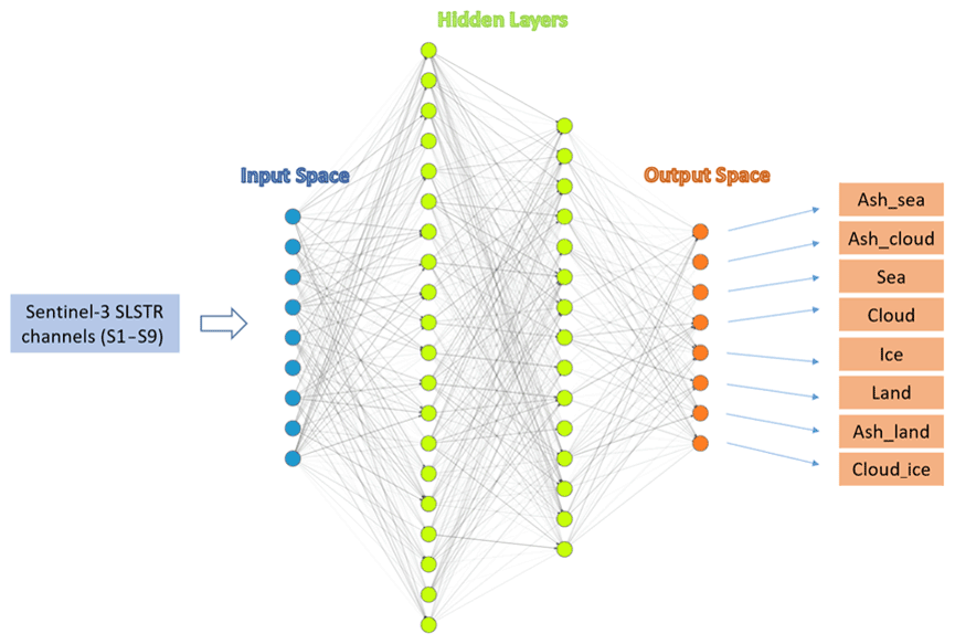
Figure 2 Overall diagram of the procedure followed for the classification process with NN model.

The MLP NN model (Atkinson and Tatnall, 1997; Gardner and Dorling, 1998) consists of a multilayer architecture with three types of layers. The first type of layer is the input layer, where the nodes represent the elements of a feature vector. The second type of layer is the hidden layer and consists of only processing units. The third type of layer is the output layer, and it represents the output data, which are the classes to be distinguished – these are set to 1 (that of the chosen class) or 0 (all other nodes) in image classification problems. All nodes (i.e., neurons) are interconnected, and a weight is associated to each connection. Each node in each layer passes the signal to the nodes in the next layer in a feed-forward way, and in this passage, the signal is modified by the weight. The receiving node sums the signals from all the nodes in the previous layer and elaborates them through an activation function before passing them to the next layer.

The output of the proposed model is the SLSTR image fully classified in eight different species: ash over sea, ash over cloud, ash over land, sea, land and ice surfaces, liquid water clouds, and ice clouds. This approach has been used because of the readily available time series of MODIS data, the quality of MODIS products (Picchiani et al., 2011, 2014; Piscini et al., 2014), and the spatial and spectral similarities between MODIS and SLSTR. The SLSTR and MODIS channels which are used in our research are shown in Table 1, along with the spectral characteristics of the two sensors.

Table 1 Correspondence between MODIS and SLSTR channels.

The first step of our procedure consists of generating the training patterns – that is, the ground truth to be passed to the NN model during the training phase. This step represents a crucial aspect in building an NN model, since the more the training dataset is accurate and representative of the problem we want to address, the more the NN would be efficient in solving that problem. For this scope, MODIS products have been used as inputs to a semi-automatic procedure for identifying the different classes to be discriminated by the NN model in the output image. Some of these classes do not exist as MODIS standard products (e.g., the ash classes and the ice surface class); for this reason, we derived them by means of different operations in our semi-automatic procedure developed in MATLAB. Other classes are, instead, already present as MODIS standard products (e.g., the land and sea mask).

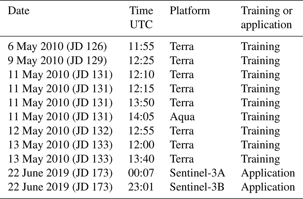
The training set from which we extracted the training patterns (i.e., identifying classification classes) consists of nine MODIS granules acquired over the Eyjafjallajökull volcano area during the 2010 eruption (from 6 to 13 May) for a total of about 5400 patterns for each class available for the training of the model. The single training pattern (i.e., training example) corresponds to a single pixel of a specific target class, as identified in MODIS images through the semi-automatic procedure aforementioned; this means that one class is represented by several patterns. In particular, not all the pixels of the MODIS images considered are contained in the training dataset (i.e., the ensemble of the training patterns), but rather, only a part of them are randomly included. The total number of patterns we collected has been divided into three subsets: 75 % training set, 20 % validation set, 5 % test set. An NN with two hidden layers was trained and then applied to Sentinel-3 SLSTR RBT (radiance and brightness temperature) Level 1 images collected during the Raikoke 2019 eruption. Table 2 shows the details of MODIS and SLSTR data used for this work.

Table 2 Training set (MODIS) from the Eyjafjallajökull 2010 eruption; Sentinel-3 SLSTR Raikoke 2019 classified products.

In order to build the NN training patterns, a semi-automatic procedure that exploits MODIS radiances and standard products has been developed. The MODIS products considered for the extraction of the training patterns are the following:

• MOD/MYD021KM, Level 1B calibrated radiances – 1 km, which gives the radiance values for each MODIS band;

• MOD/MYD03, geolocation – 1 km, which is used for creating the land and sea mask;

• MOD/MYD06_L2, cloud product, which contains cloud parameters used for creating the cloud mask;

• MOD/MYD09, surface reflectance product, which contains an estimate of the surface spectral reflectance measured at ground level; it is used for generating the ice mask.

It is noted that “MOD” and “MYD” stand for MODIS-Terra and MODIS-Aqua products, respectively.

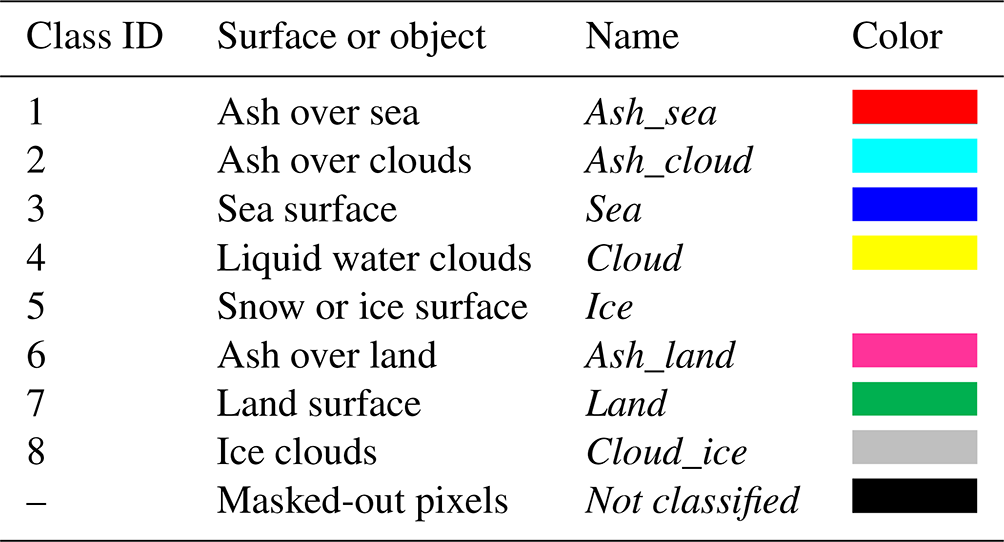
The semi-automatic procedure for the extraction of training patterns starting from MODIS data basically consists of using MODIS products to create binary “masks” identifying the different species and then replacing them with “classes”. For each element of the class, the radiance values (W (m² sr µm)⁻¹) are extracted from the MODIS product MOD/MYD021KM. In this way, each object is radiometrically characterized. The identification of the ashy pixel is pursued by creating a mask according to specific BTD thresholds (from 0.0 to −0.4 ^∘C) for each MODIS image. For this purpose, the MOD/MYD021KM product has been used to derive the brightness temperatures required to compute the BTD. The MODIS products used for training the model were acquired in near-nadir view only. The other species are identified using both MODIS Level 1 radiances and MODIS standard products. Once each object and surface has been defined, they are associated with the corresponding class. Then a set of input–output samples for the training phase is generated, where the input consists of the set of radiances measured for the given pixel and where the output is a binary vector with value 1 associated with the corresponding class and value 0 for the other classes. Table 3 shows the classification map legend for each classified product presented in this work, in which eight classes are discriminated, each one representing a surface or object.

Table 3 Classification map legend.

The NN final model consists of nine inputs, which are the radiances in the SLSTR selected channels, while the output space is composed of eight classes, which are the surfaces which the net has to classify. After doing several tests, the optimum topology of the NN turns out to be the combination of two hidden layers with 20 and 15 neurons, respectively. For each neuron, we set the hyperbolic tangent activation function (Vogl et al., 1988). The final neural network architecture used for ash detection in this work is shown in Fig. 3. The proposed algorithm includes a post-processing operation in order to avoid false positive results for land and sea classes. This a posteriori filter is applied to both the resulting NN land and sea classes. It allows for the masking out of the pixels which the NN classifies as land or sea which do not belong to the Sentinel-3 SLSTR land and sea mask standard product, which is always available and can thus be used to increase the precision of the algorithm. The filtered-out pixels have been inserted in a class named “not classified”, as reported in Table 3. For classification problems approached with machine learning algorithms, one of the most used accuracy metrics for the performance evaluation is the confusion matrix (Fawcett, 2006), where each predicted output class is compared to the corresponding ground truth considered in the validation dataset. An overall accuracy of 90.9 % was obtained at the end of the NN training phase for the proposed neural network model (see Fig. 4).

Figure 3 NN topology for ash detection.

Figure 4 Confusion matrix on validation set.

The target class represents the ground truth of each class, while the output class refers to the prediction of the NN. The diagonal shows that most of the total of the pixels have been correctly classified (green boxes). The number of pixels incorrectly classified are placed out of the diagonal. False positives (false detection) and false negatives (missed detection) are reported in the last gray column and row, respectively. The code of the procedure ran with a CPU i7-9850H (6 core, processor base frequency at 2.60 GHz): it takes less than 30 min to train the adopted model and a few seconds to apply it.

5 Results and discussion

The neural network algorithm previously described was applied to Sentinel-3 SLSTR daytime images acquired for Raikoke during the 2019 eruption. The Sentinel-3A SLSTR and Sentinel-3B SLSTR products collected on 22 June 2019 at 00:07 and 23:01 UTC, respectively, have been considered (see Table 2).

Figure 5a shows the RGB color composite of the S3A SLSTR image acquired for Raikoke for 22 June 2019 at 00:07 UTC. The RGB composite has been carried out by considering the SLSTR visible (VIS) channels S3 (868 nm), S2 (659 nm), and S1 (554 nm) for R, G, and B, respectively. In Fig. 5b, the BTD map – where red and blue pixels represent negative and positive BTD, respectively – is displayed. The BTD is computed by making the difference between the brightness temperature of the SLSTR thermal infrared channels S8 and S9 centered at 10.8 and 12 µm, respectively. The output of the NN classification is shown in Fig. 5c with the corresponding color legend, where each color represents the classified surface or object.

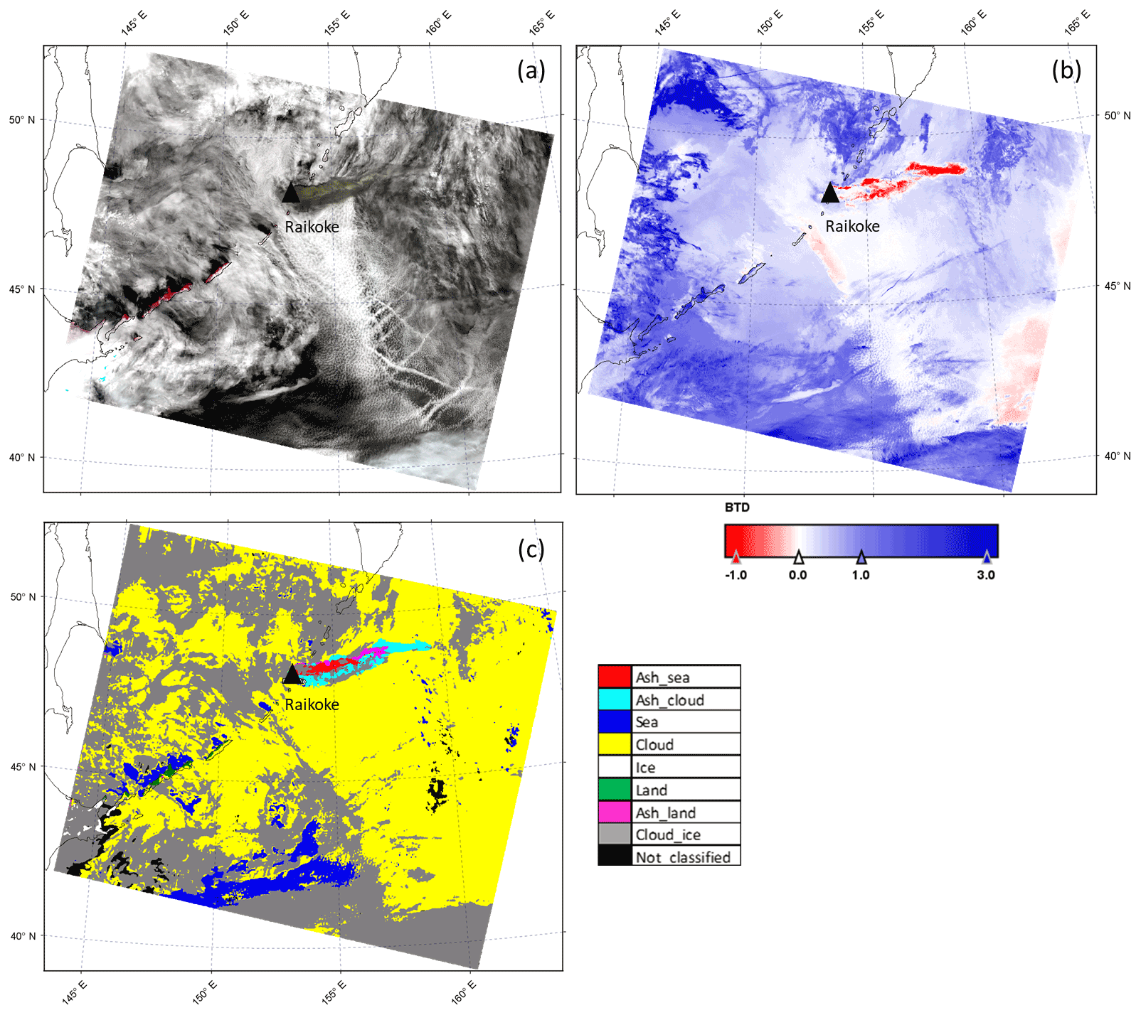
Figure 5 S3A SLSTR image collected for Raikoke on 22 June 2019 at 00:07 UTC, nadir view. (a) RGB; (b) BTD; (c) NN classification.

As Fig. 5a shows, the RGB composite shows the presence of a wide distribution of meteorological clouds and a significant signal derived from the volcanic cloud (brown pixels). The BTD (Fig. 5b), obtained with a threshold of 0 ^∘C, shows the presence of the volcanic cloud together with a significant number of false negatives (volcanic cloud pixels not identified near the vents) and false positives (pixels identified as volcanic cloud while, actually, they are not – see light red pixels below the volcanic cloud and along the right edge of the scene).

Despite the challenging scenario, the NN algorithm shows its ability to detect volcanic cloud and to classify the whole image by detecting with good accuracy meteorological clouds composed of water droplets (yellow) and ice (gray), sea (blue) and land (green) surfaces, and volcanic ash clouds, as reported in Fig. 5c. Looking at the cloud masks generated with the NN algorithm (yellow and gray) and by comparing them with the RGB natural color composite of the SLSTR product, a high degree of agreement in terms of spatial features can been observed. From the comparison between NN output classes and RGB composite, we can also observe that land (green) and sea (blue) pixels are properly detected in the areas where they actually lie.

From a qualitative comparison between the NN plume mask and the RGB composite, we can state that the NN correctly identifies the volcanic cloud class in the area where it seems actually present, even if some pixels are misclassified as ash over land (magenta pixels) instead of ash above meteorological cloud. As Fig. 5 shows, the NN algorithm is able to detect a wide volcanic cloud area and more ash, especially in the opaque regions, compared to the BTD approach. In particular, the difference found near the vents could be due to the complete opacity of the cloud. Here, the ash cloud optical thickness is so high that there is no spectral difference, and the BTD approach has no sensitivity.

Following the same visualization scheme as Fig. 5, the results derived from the application of the trained NN model to the S3B SLSTR image acquired on 22 June 2019 at 23:01 UTC are reported in Fig. 6. In this second image, all the ashy pixels are classified by the NN model as ash above meteorological clouds (cyan pixels). This seems reasonable, being the scenario mostly dominated by meteorological clouds, as we can also observe looking at the NN classification, which assigns the majority of the pixels to the liquid water cloud class (yellow) and to the ice cloud class (gray). The NN classification also shows the presence of sea pixels (blue), which are located in the same area identifiable using the RGB composite. In this case, from the RGB composite (Fig. 6a), unlike what is seen in the 00:07 UTC image, it is not straightforward to identify the volcanic plume by visual inspection. Indeed, this image was collected about 24 h later than the previous one, and thus, the plume has been transported through the atmosphere and dispersed. A qualitative comparison between the NN classification (Fig. 6c) and the BTD map (Fig. 6b) shows considerable differences between the two methods. The BTD, obtained with a threshold of 0 ^∘C, identifies a wider area (red pixels) affected by the volcanic cloud with respect to the NN ash mask (cyan pixels). We can notice that the BTD map includes some aircraft condensation trails (recognizable by the shape in the RGB composite) in the ash mask, which can be identified as false ash detections. The reasons for these misclassifications are not fully understood but may be due to multilayer cloud effects, pixel heterogeneity, or viewing angle.

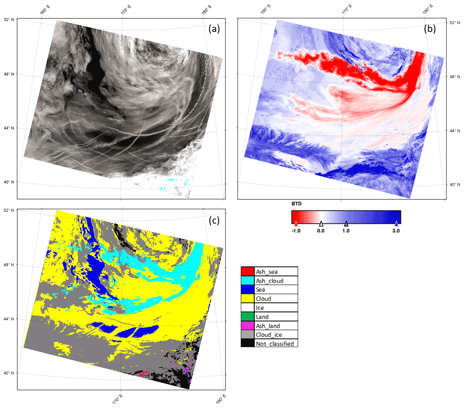
Figure 6 S3B SLSTR image collected for Raikoke on 22 June 2019 at 23:01 UTC, nadir view. (a) RGB, (b) BTD, (c) NN classification.

Our results suggest that the NN technique is robust and have shown that it is possible to transfer the NN model from one single eruption event to others occurring at similar latitudes. However, the complexity of the application suggests that the generalization of the methodology to all types of eruptions is not straightforward. For example, the change of latitude has an impact on the characteristics of the atmosphere. At the same time, different volcanoes emit different types of ash, affecting the variability of the radiance values detected by the sensors. A possible solution to give the proposed technique a broader applicability could be to train different NN models for specific latitude belts, which can then be defined to cover the whole globe.

Overall, we can summarize the main uncertainties and the limitations of the presented model in the following points:

1. Model transferability is significantly related to the spatial-temporal data availability for the generation of a training dataset which is statistically representative of all the possible scenarios.

2. The lack of standard ground truth data for training and validation phases requires that the BTD threshold be selected by an operator, which prevents the method from being fully objective.

Vicarious validation

The capability of the NN to correctly detect pixels containing ash was validated by making a pixel-per-pixel comparison with a manually generated reference plume mask (hereafter MPM) in order to obtain the most accurate ground truth as possible in each SLSTR product. The choice of taking the MPM as a reference is derived from the lack of ash standard products. For the image collected at 00:07 UTC, the MPM creation was performed by selecting a region around the volcanic cloud (clearly recognizable, as it is at the beginning of the eruption) and then considering only the pixels with 11 µm brightness temperature <270 K (see Fig. 1). In this case, the BTD alone is not very useful, as the high value of the ash optical thickness of the cloud (especially close to the vent) produces many pixels with BTD values near 0, not distinguishable from adjacent pixels characterized by meteorological clouds. For the image collected at 23:01 UTC, the identification of the volcanic cloud is much more difficult due to its larger spread and dilution; in this case, the MPM was obtained considering the pixels with BTD $<-\mathrm{0.25}$ ^∘C, even if this choice probably implies that some ashy pixels were discarded. On the other hand, using a higher BTD threshold will produce a lot of false positive pixels. In general, the creation of an accurate manual plume mask is time consuming and case sensitive and often requires the presence of an operator; considering this, the generation of a volcanic cloud mask with a fast, automatic, and case-independent procedure would be a rather significant improvement. Because the MPM does not distinguish between the different surfaces under the ash cloud, the validation is performed by considering the total of the ashy pixels detected from the NN (i.e., the sum between ash_land, ash_sea and ash_cloud).

Figure 7 shows the MPM, created as described above, and the comparison between the NN plume mask (hereafter NNPM) and the MPM for the S3A SLSTR image collected for Raikoke on 22 June 2019 at 00:07 UTC (Fig. 7a and b) and the S3B SLSTR image collected for Raikoke on 22 June 2019 at 23:01 UTC (Fig. 7c and d).

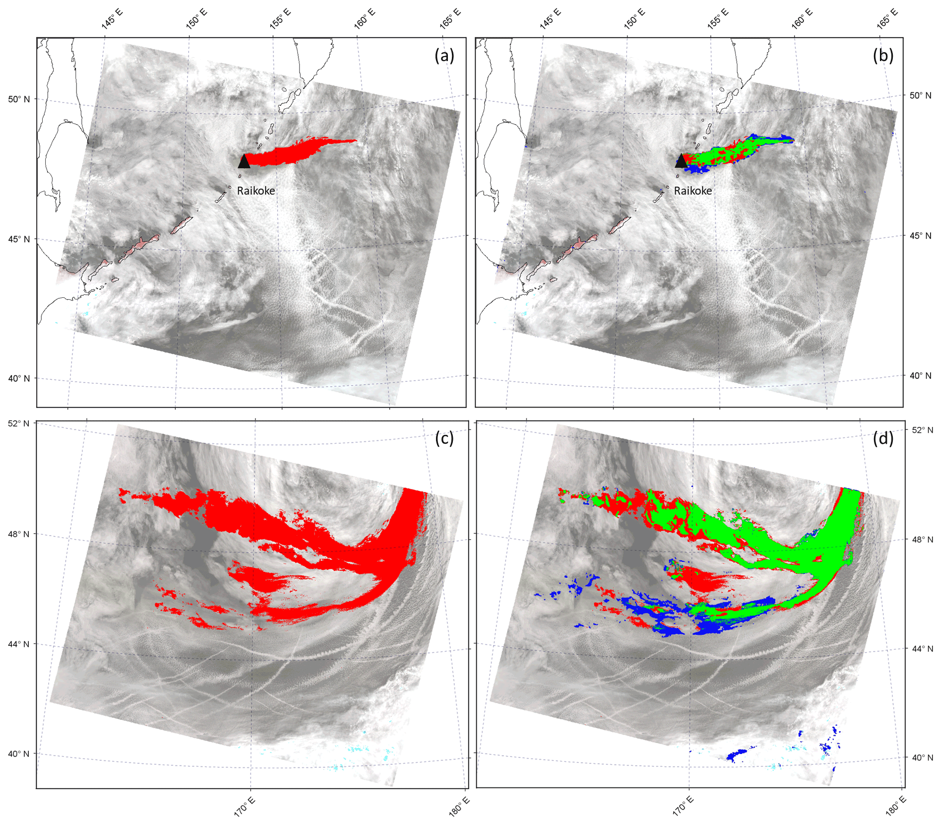
Figure 7 (a) Manual plume mask (MPM) obtained from the analysis of the S3A SLSTR image collected for Raikoke on 22 June 2019 at 00:07 UTC (nadir view) – red pixels identify the MPM; (b) comparison between volcanic ash detected by NN and MPM for the S3A SLSTR image collected for Raikoke on 22 June 2019 at 00:07 UTC (nadir view); (c) MPM obtained from the analysis of the S3B SLSTR image collected for Raikoke on 22 June 2019 at 23:01 UTC (nadir view) – red pixels identify the MPM; (d) comparison between volcanic ash detected by NN and MPM for the S3B SLSTR image collected for Raikoke on 22 June 2019 at 23:01 UTC (nadir view). (b, d) Green pixels indicate the areas for which both NN and MPM detect ashy pixels; red pixels indicate the areas for which only MPM detects ashy pixels; blue pixels indicate the areas for which only NN detects ashy pixels.

In relation to the images which display the comparison between NN output and MPM (Fig. 7b and d), green areas indicate the pixels for which both the MPM and NN ash masks detect the presence of volcanic cloud; red pixels represent the areas classified as ash only by the MPM; blue pixels are classified as ash only according to the NN model. We can observe that most of the volcanic cloud is displayed in green for both products (00:07 and 23:01 UTC), indicating good agreement between the two approaches. This is also confirmed by the scores in Table 4, which allow quantitative conclusions regarding the accuracy of the proposed NN model approach compared to the MPM considered as ground truth. The classification metrics considered are precision, recall, F-measure, and accuracy (Fawcett, 2006), which range from 0 to 1 (perfect classifier).

Table 4 NN and BTD volcanic cloud detection accuracies using classification metrics derived from the comparison between the plume mask obtained from the two approaches and the manual plume mask (MPM) for each SLSTR considered product, respectively.

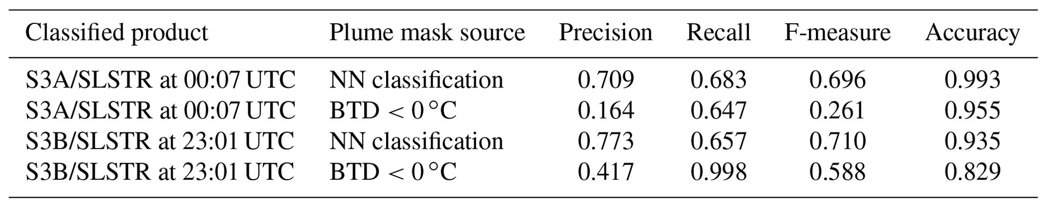
The score differences for the two classified products are mainly related to the significant higher number of correctly classified ashy pixels contained in the 23:01 UTC (136 435 pixels) with respect to 00:07 UTC (13 545 pixels) if compared to the total number of classified pixels in the images which are similar (1 614 405 pixels for the S3A SLSTR at 00:07 UTC image and 1 701 319 for the S3B SLSTR at 23:01 UTC image, respectively). However, the metrics are aligned for both classified data, with encouraging values for each index suggesting the reasonability of the results. In particular, the F-measure results are around 0.7 for both classifications. Moreover, using MPM as a benchmark, the comparison of the metrics obtained with the BTD <0 ^∘C approach with those derived with the NN model indicates that the neural network performs a more accurate volcanic cloud detection for both considered test cases.

Besides the NN plume mask validation, we also compared the pixels which the NN model classified as being affected by meteorological clouds (hereafter referred to as NNCM) with the SLSTR standard product for meteorological clouds. Among the cloud masks available in the SLSTR L1RBT product, the confidence_in_summary_cloud mask (hereafter CSCM) is considered. The CSCM is a cloud mask which discriminates cloud pixels (true) and cloud-free pixels (false); it is an ultimate cloud mask product derived from several separated cloud tests (Polehampton et al., 2021). As the CSCM does not distinguish between meteorological liquid water clouds and meteorological ice clouds while the NN algorithm does, the comparison is realized by considering the whole of the NN meteorological cloud classes (i.e., the sum between Cloud and Cloud_ice).

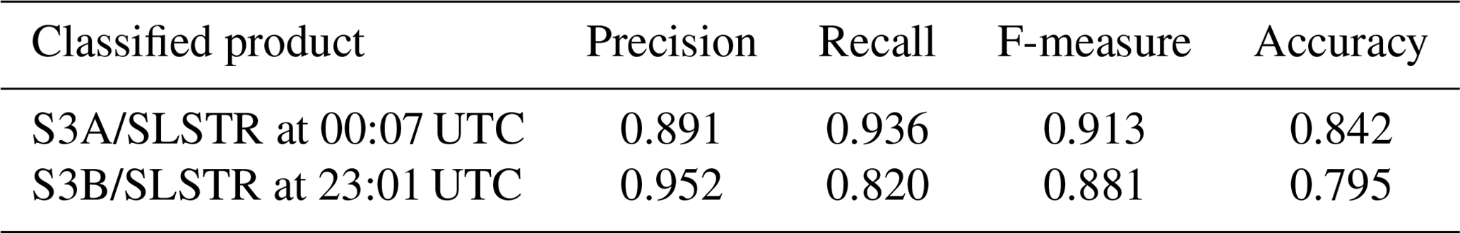
Figure 8 displays the RGB composite, in which the Sentinel-3 sun glint mask is highlighted (right part of the scene), and the comparison between NN cloud mask and S3 cloud mask for the S3A SLSTR image collected for Raikoke on 22 June 2019 at 00:07 UTC (Fig. 8a and b) and for the S3B SLSTR image collected for Raikoke on 22 June 2019 at 23:01 UTC (Fig. 8c and d). Also in this case, for the images displaying the comparison between the two types of cloud masks (Fig. 8b and d), green indicates the pixels classified as meteorological cloud for both procedures, while red and blue indicate the pixels classified as meteorological cloud only by the SLSTR standard product and NN, respectively. Pixels that are not colored are associated with a cloud-free condition for both the NN and the S3 cloud mask. Looking at the comparison, a very good agreement between the NN meteorological cloud mask and the SLSTR standard cloud mask can be observed. The metrics in Table 5 show very good performance, reaching an F-measure around 0.9. Moreover, looking at the red pixels in the 23:01 UTC image especially, it can be noted that the SLSTR cloud mask also includes the volcanic cloud.

Figure 8 (a) S3A SLSTR image collected for Raikoke on 22 June 2019 at 00:07 UTC (nadir view), RGB color composite; (b) comparison between cloud mask retrieved by NN and standard Sentinel-3 confidence-in-summary cloud mask (CSCM) for the S3A SLSTR image collected for Raikoke on 22 June 2019 at 00:07 UTC (nadir view); (c) S3B SLSTR image collected for Raikoke on 22 June 2019 at 23:01 UTC (nadir view), RGB color composite; (d) comparison between cloud mask retrieved by NN and standard CSCM for the S3B SLSTR image collected for Raikoke on 22 June 2019 at 23:01 UTC (nadir view). (b, d) Green pixels indicate the areas for which both NN and CSCM detect cloudy pixels; red pixels indicate the areas for which only CSCM detects cloudy pixels; blue pixels indicate the areas for which only NN detects cloudy pixels; white pixels indicate the areas for which neither NN nor CSCM detect cloudy pixels.

Table 5 NN meteorological cloud detection accuracy using classification metrics derived from the comparison between the NN cloud mask (NNCM) and the confidence-in-summary cloud mask (CSCM) for each SLSTR product considered which has been assumed as ground truth.

From the validation procedure we have carried out, a considerable point which has to be underlined is that, unlike adopting a time-consuming and case-specific approach like MPM, which also needs a manual operation by setting various thresholds for each case under examination, the NN model can be used to discriminate ash plumes in satellite images with good accuracy in a fast and automatic way. This saves a significant amount of time by eliminating the need for manual intervention.

6 Conclusions

In this work, the results of a new neural-network-based approach for volcanic cloud detection are described. The algorithm, developed to process Sentinel-3 SLSTR daytime images, exploits the use of MODIS daytime data as training. The procedure allows the full characterization of the SLSTR image by identifying, besides volcanic cloud, surfaces under the cloud itself, meteorological clouds (and phases), and land and sea surfaces. As test cases, the S3A-S3B SLSTR images collected over the Raikoke volcano area during the June 2019 eruption have been considered. The proposed neural-network-based approach for volcanic ash detection and image classification shows an overall good accuracy for the ash class, which is the main target of the algorithm, and for the meteorological cloud class. The strong effectiveness of the NN classification is indeed also related to the cloudy pixel recognition, with the ability to distinguish between two different types of meteorological clouds composed of water droplets and ice, respectively. It has to be remembered that the wide distribution of meteorological clouds in the scenario under consideration makes the ash detection task particularly complex.

A point to be underlined is the valuable advantage of the procedure with regard to the creation of products (the eight classes) that are not all currently available as SLSTR standard products; this fact represents a considerable step forward for the generation of novel types of S3 SLSTR products.

A post-processing has been applied to NN outputs by exploiting the land and sea mask available in the SLSTR standard products in order to mitigate the insurgence of NN land and sea failure. The comparison between the NN plume mask and a reference plume mask (MPM) taken as ground truth shows a good agreement between the two techniques (F-measure of around 0.7). This significant result lies in the fact that the overall good performance of the NN output is achieved in an automatic way and with a brief processing time compared to the plume mask specifically generated, which instead requires a longer time, is case specific, and requires the presence of an operator. The other considerable achievement of the NN procedure is that, once the NN model has been properly trained, it can be used to detect the ash plume for each SLSTR image related to the Raikoke eruption, while the creation of the MPM has to be made separately for each image. The comparison between the NN cloud mask and the cloud mask derived from SLSTR standard products has also been carried out, resulting in a high percentage of agreement between the two products.

A promising outcome is related to the ability of the NN model to generalize over different data in terms of spatio-temporal and geographical characteristics, being the NN model trained with data collected over the Iceland region in 2010 and then applied to data acquired over the Kamchatka Peninsula in Russia in 2019. Something under consideration for future improvements is to enhance the ability of the NN to generalize over various eruptive scenarios by integrating different training datasets (in terms of regions, type of eruption, time interval, etc). In fact, the current methodology has been applied to just a few test cases, and more validation is required in order to give the technique broader applicability. For example, the effects of varying moisture and atmospheric conditions has not been fully explored. On the other hand, the generation of an appropriate number of examples, which must be statistically representative of all the possible scenarios, to be included in the training dataset may represent a very difficult task. A possible approach could be the design of different neural networks, each associated with a specific scenario.

We also aim at further investigating some aspects in order to improve the classification accuracy, such as the introduction of other output classes – such as volcanic ice clouds – and the integration of other variables in the model – such as the sensor view angle.

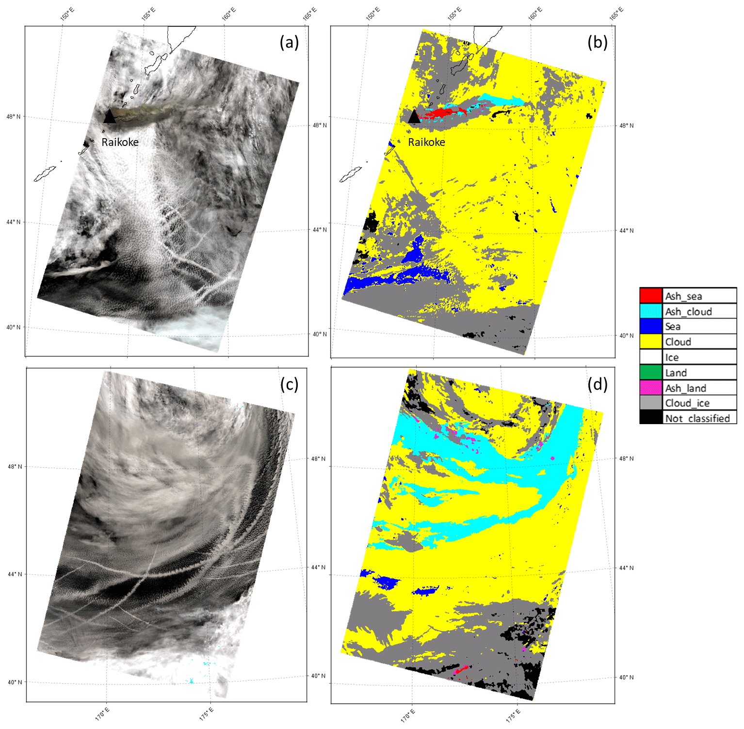
Figure 9 (a, b) S3A SLSTR image collected for Raikoke on 22 June 2019 at 00:07 UTC, oblique view; (c, d) S3B SLSTR image collected for Raikoke on 22 June 2019 at 23:01 UTC, oblique view. (a, c) RGB; (b, d) NN classification.

Moreover, a fully comprehensive study of the sensitivity of the NN detection on the observation angle could be another possible future development of the study. Here, we briefly addressed this point by applying the trained network to SLSTR oblique-view products, characterized by a view zenith angle of about 55^∘ (Polehampton et al., 2021). Figure 9 shows the RGB composite and the NN classification for the SLSTR oblique-view product collected on 22 June 2019 at 00:07 UTC (Fig. 9a and b) and 23:01 UTC (Fig. 9c and d), respectively. It is interesting, as a preliminary result, to show how the main features of the classification map obtained using a NN model trained only on near-nadir-view-acquired products and used for classifying oblique view data are mostly conserved, especially for the 23:01 UTC image, where the opacity of the volcanic cloud is lower. However, the complexity brought in by the difference in the slant optical depth, which may translate to a noticeable difference in top-of-atmosphere signal levels, needs to be investigated in a full, dedicated study. Finally, the possibility of using S3 SLSTR products to train a neural network that is able to detect volcanic clouds in Sentinel-3 SLSTR granules might improve the overall accuracy of the classification.