the Creative Commons Attribution 4.0 License.
the Creative Commons Attribution 4.0 License.
 | 20 Dec 2022
Quantification of primary and secondary organic aerosol sources by combined factor analysis of extractive electrospray ionisation and aerosol mass spectrometer measurements (EESI-TOF and AMS)
Yandong Tong
Lu Qi
Giulia Stefenelli
Dongyu Simon Wang
Francesco Canonaco
Urs Baltensperger
André Stephan Henry Prévôt
Jay Gates Slowik
Source apportionment studies have struggled to quantitatively link secondary organic aerosols (SOAs) to their precursor sources due largely to instrument limitations. For example, aerosol mass spectrometer (AMS) provides quantitative measurements of the total SOA fraction but lacks the chemical resolution to resolve most SOA sources. In contrast, instruments based on soft ionisation techniques, such as extractive electrospray ionisation mass spectrometry (EESI, e.g. the EESI time-of-flight mass spectrometer, EESI-TOF), have demonstrated the resolution to identify specific SOA sources but provide only a semi-quantitative apportionment due to uncertainties in the dependence of instrument sensitivity on molecular identity. We address this challenge by presenting a method for positive matrix factorisation (PMF) analysis on a single dataset which includes measurements from both AMS and EESI-TOF instruments, denoted “combined PMF” (cPMF). Because each factor profile includes both AMS and EESI-TOF components, the cPMF analysis maintains the source resolution capability of the EESI-TOF while also providing quantitative factor mass concentrations. Therefore, the bulk EESI-TOF sensitivity to each factor can also be directly determined from the analysis. We present metrics for ensuring that both instruments are well represented in the solution, a method for optionally constraining the profiles of factors that are detectable by one or both instruments, and a protocol for uncertainty analysis.
As a proof of concept, the cPMF analysis was applied to summer and winter measurements in Zurich, Switzerland. Factors related to biogenic and wood-burning-derived SOAs are quantified, as well as POA sources such as wood burning, cigarette smoke, cooking, and traffic. The retrieved EESI-TOF factor-dependent sensitivities are consistent with both laboratory measurements of SOA from model precursors and bulk sensitivity parameterisations based on ion chemical formulae. The cPMF analysis shows that, with the standalone EESI-TOF PMF, in which factor-dependent sensitivities are not accounted for, some factors are significantly under- or overestimated. For example, when factor-dependent sensitivities are not considered in the winter dataset, the SOA fraction is underestimated by ∼25 % due to the high EESI-TOF sensitivity to components of primary biomass burning such as levoglucosan. In the summer dataset, where both SOA and total OA are dominated by monoterpene oxidation products, the uncorrected EESI-TOF underestimates the fraction of daytime SOA relative to nighttime SOA (in which organonitrates and less oxygenated CxHyOz molecules are enhanced). Although applied here to an AMS and EESI-TOF pairing, cPMF is suitable for the general case of a multi-instrument dataset, thereby providing a framework for exploiting semi-quantitative, high-resolution instrumentation for quantitative source apportionment.
- Article
(6207 KB) - Full-text XML
-
Supplement
(9313 KB) - BibTeX
- EndNote


Atmospheric aerosols negatively affect visibility (Watson, 2002), human health (Pope et al., 2002; Laden et al., 2006; Beelen et al., 2014), and urban air quality (Fenger, 1999; Mayer, 1999) on local and regional scales. Aerosols also provide the largest uncertainties for global radiation balance and climate change (Lohmann and Feichter, 2005; Forster et al., 2007; Penner et al., 2011; Myhre et al., 2013). Therefore, to develop appropriate mitigation policies, it is of vital importance to understand aerosol chemical composition, sources, and evolution. Organic aerosols (OAs) are a major component of atmospheric aerosols and account for 20 % to 90 % of the submicron aerosol mass (Jimenez et al., 2009). OAs are typically classified as either primary organic aerosols (POAs), which are directly emitted to the atmosphere, or secondary organic aerosols (SOAs), which are produced by atmospheric reactions of emitted volatile organic compounds (VOCs). Both POAs and SOAs can exert serious health effects, including protein and DNA damage caused by reactive oxygen species (ROS), which can be either contained in the particles or induced by oxidation reactions following inhalation (Halliwell and Cross, 1994; Li et al., 2003; Reuter et al., 2010; Kelly and Fussell, 2012; Fuller et al., 2014). Recent studies indicate that the oxidation potential of SOAs is source dependent. Therefore, different sources likely carry different health risks, highlighting the importance of OA source identification and quantification (Zhou et al., 2018; Daellenbach et al., 2020). Previous studies have been relatively successful in quantitatively linking POAs to their sources. However, quantification of SOA sources and/or formation pathways is more challenging due to (1) the chemical complexity of SOA, which can consist of thousands of unique oxidation products, including highly oxygenated molecules and high molecular weight organic oligomers, and (2) the limitations of traditional instrumentation for characterising OA chemical composition, especially the SOA fraction. Therefore, the effects of individual SOA sources on health and climate remain poorly constrained.
Positive matrix factorisation (PMF) is a widely used source apportionment technique. PMF is a bilinear receptor model which represents the measured mass spectral time series as a linear combination of factor mass spectra and their corresponding time-dependent concentrations (Paatero and Tapper, 1994). These factors may then be related to emission sources and/or to atmospheric processes, depending on their chemical and temporal characteristics. PMF has been implemented in extensive online and offline studies worldwide to quantify OA sources. The Aerodyne aerosol mass spectrometer (AMS) is widely used in OA source apportionment studies, because it provides online, quantitative measurements of non-refractory PM1 or PM2.5 (particulate matter with an aerodynamic diameter smaller than 1 or 2.5 µm, respectively) chemical composition with high time resolution. Source apportionment studies using PMF based on AMS data have successfully separated and quantified POA sources based on different chemical signatures, e.g. hydrocarbon-like OA (HOA) (Ng et al., 2011b; Zhang et al., 2014; Elser et al., 2016; Sun et al., 2016a; Xu et al., 2019; Zhao et al., 2019), cooking-related OA (COA) (Mohr et al., 2012; Crippa et al., 2013b; Hu et al., 2016; Sun et al., 2016a, b; Xu et al., 2019; Zhao et al., 2019), biomass-burning OA (BBOA) (Alfarra et al., 2007; Lanz et al., 2007; Sun et al., 2011), and coal combustion OA (CCOA) (Zhang et al., 2008, 2014; Elser et al., 2016; Hu et al., 2016; Sun et al., 2016a). However, SOAs are typically reported as either a single SOA factor (denoted oxygenated organic aerosol, OOA) or as two factors distinguished by degree of oxygenation (i.e. less oxygenated OOA, LO-OOA, and more oxygenated OOA, MO-OOA) or by volatility (i.e. semi-volatile OOA, SV-OOA, and low-volatility OOA, LV-OOA) (Jimenez et al., 2009; Zhang et al., 2011; Crippa et al., 2013b; Sun et al., 2013; Elser et al., 2016; Sun et al., 2016a; Xu et al., 2019) rather than in terms of sources and/or formation processes. This limitation is due to the vaporisation and ionisation scheme in the AMS, which causes significant thermal decomposition and ionisation-induced fragmentation (DeCarlo et al., 2006). The corresponding decrease in chemical resolution, particularly for multifunctional and/or highly oxygenated SOA components (e.g. multifunctional acids, peroxides, organonitrates, organosulfates, oligomers), limits the resolution of SOA source apportionment.
The development of continuous or semi-continuous instruments with softer vaporisation and ionisation schemes has provided new insights into SOA composition and is thus of considerable interest for source apportionment. Recent examples include the (semi-continuous) Filter Inlet for Gases and AEROsols chemical ionisation time-of-flight mass spectrometer (FIGAERO-CIMS) (Lopez-Hilfiker et al., 2014) and the (continuous) extractive electrospray ionisation time-of-flight mass spectrometer (EESI-TOF) (Lopez-Hilfiker et al., 2019), which implement soft ionisation schemes at lower temperatures than the AMS, thereby reducing thermal decomposition and increasing chemical resolution (i.e. providing chemical formulae of molecular ions). A recent source apportionment study using a FIGAERO-CIMS at a rural site in the southeastern USA successfully resolved three SOA factors, characterised by isoprene-derived species such as carboxylic acids from aqueous phase processes, highlighting the chemistry of biogenic species (Chen et al., 2020). Another source apportionment study from Lee et al. (2020) using FIGAERO-CIMS spectra successfully distinguished ambient SOA formation and ageing pathways into two forested regions. Source apportionment studies in Zurich using an EESI-TOF identified SOA factors from monoterpene oxidation in summer (Stefenelli et al., 2019) and oxidation of biomass-burning emissions in winter (Qi et al., 2019). EESI-TOF measurements identified SOA factors related to solid fuel combustion and aqueous-phase processes in Beijing (Tong et al., 2021) and SOA factors with aromatic and biogenic origins in Delhi (Kumar et al., 2022). However, to date, the factor concentrations returned by PMF analyses using these instruments are not quantitative.
Quantification of the measurements by instruments such as EESI-TOF and CIMS is challenging, because the instrument sensitivity varies strongly with molecular identity. For CIMS, the sensitivity to different compounds is determined by the frequency of collisions between reagent ions and analytes, the ion–molecule reaction time, and the transmission efficiency of product ions to the detector, which depends on ion–molecule binding energy. Lopez-Hilfiker et al. (2016) developed methods to estimate the binding energy of iodide (I−) adduct ions of multifunctional organic compounds for species whose formation is collision limited, providing a lower limit to their mass concentrations. Another method to explore the sensitivity is to measure single-compound aerosols or SOAs generated from different precursors by an EESI-TOF and a scanning mobility particle sizer (SMPS) simultaneously to determine the mass concentration (Lopez-Hilfiker et al., 2016). Lopez-Hilfiker et al. (2019) explored EESI-TOF sensitivities to selected reference compounds with different functional groups (including saccharides, polyols, and carboxylic acids) and bulk SOAs generated from oxidation of a single precursor VOC. For pure compounds, relative sensitivities vary by 2 orders of magnitude, with some composition-dependent trends evident (e.g. increasing sensitivity of saccharides with decreasing molecular weight and high sensitivities for polyols relative to other functionalities). In addition, a trend of decreasing sensitivity with decreasing molecular weight of the precursors was found for bulk SOAs. While calibration with standard compounds is straightforward, the quantification of individual species within SOAs is extremely challenging due to their complex composition, the lack of chemical standards for most molecules, and the potential for structural isomers to have significantly different sensitivities. These issues were investigated recently for the EESI-TOF by generating SOAs in the presence of a variable seed surface area and comparing the difference in SOA ion concentrations measured by the EESI-TOF and the corresponding gas-phase concentrations measured by a Vocus proton transfer reaction mass spectrometer (Vocus-PTR-MS) (Wang et al., 2021). The observed sensitivities for different SOA components produced from the oxidation of limonene, o-cresol, or 1,3,5-trimethylbenzene ranged from 103 to 105 ion s−1 ppb−1. A regression model was developed that was able to predict the ion-by-ion sensitivities to within a factor of 5 of the experimental value when the precursor VOC is known a priori. However, the study also showed significantly different sensitivities (up to a factor of 20) for structural isomers derived from different VOC precursors. Similar isomer sensitivity differences for the I−-CIMS were also reported by Bi et al. (2021). The fact that these isomers cannot be distinguished by 1-D mass spectrometry represents a fundamental limitation of calibration- and parameterisation-based quantification and complicates interpretation of the binding energy-based approach (Lopez-Hilfiker et al., 2016), because ambient SOAs may derive from unknown or complex mixtures of VOCs. Therefore, for source apportionment purposes, source-based sensitivities are preferred and essential to quantify SOA sources and formation processes.
Here, we present a new approach for quantification of SOA sources retrieved from source apportionment. This is achieved by PMF analysis of a single input matrix consisting of data from both a quantitative instrument with a lower chemical resolution (i.e. AMS) and an instrument with a high chemical resolution and a linear but molecule-dependent response (i.e. EESI-TOF). This method is based on the combined PMF (cPMF) analysis previously performed on combined OA and VOC data from AMS and PTR-MS, respectively (Slowik et al., 2010; Crippa et al., 2013a) but utilises a more robust metric for ensuring adequate representation of both instruments in the model solution, optionally allows constraints to be placed on the factor profile contributions for one or both instruments, and provides a method for uncertainty analysis. The cPMF method is applied to AMS/EESI-TOF datasets collected during summer and winter campaigns in Zurich, Switzerland, for which single-instrument PMF analyses were previously reported (Qi et al., 2019; Stefenelli et al., 2019). The present study is the first application of cPMF to a joint EESI-TOF–AMS dataset and the first quantitative EESI-TOF-driven source apportionment.
2.1 The measurement site and field campaigns
Field campaigns were conducted at the Swiss National Air Pollution Monitoring Network (NABEL) station, an urban background site located in the Alte Kaserne, central Zurich (47∘22′ N, 8∘33′ E, 410 m above sea level), previously described in detail (Lanz et al., 2007; Canonaco et al., 2013). The measurements used in the current analysis are from 20 to 26 June 2016 and 25 January to 4 February 2017. These periods are excerpted from longer campaigns and correspond to the times during which both the AMS and EESI-TOF achieved stable operation. The measurement site is located in a courtyard, although influences from nearby restaurants, local minor roads, and human activities (e.g. cigarette smoking) are often observed (Lanz et al., 2007; Daellenbach et al., 2017; Qi et al., 2019; Stefenelli et al., 2019; Qi et al., 2020). Gas-phase species – e.g. nitrogen dioxide (NO2), nitrogen oxide (NO), and sulfur dioxide (SO2) – and meteorological data – e.g. temperature (T), relative humidity (RH), radiation, wind speed (WS), and wind direction (WD) – are recorded by the monitoring station.
During the intensive campaigns, a separate trailer was deployed to house an additional suite of gas and particle instrumentation. A PM2.5 cyclone was installed ∼75 cm above the trailer roof (∼5 m above ground) to remove coarse particles. After passing through the cyclone, the sampled air passed through a stainless-steel (∼6 mm outer diameter, O.D.) tube to the particle instrumentation, which included a high-resolution time-of-flight aerosol mass spectrometer (HR-TOF-AMS, Aerodyne Research Inc.) and an extractive electrospray ionisation time-of-flight mass spectrometer (EESI-TOF) to measure the OA composition, and a scanning mobility particle sizer (SMPS) to measure the particle concentration and size distribution. The summer and winter campaign results, including OA source apportionment from the standalone AMS and EESI-TOF datasets, were previously presented in detail (Qi et al., 2019; Stefenelli et al., 2019). In this study, we focus on the OA source apportionment using positive matrix factorisation (PMF) on the combined dataset from AMS and EESI-TOF, collected during the two campaigns.
2.2 Instrumentation
2.2.1 High-resolution time-of-flight aerosol mass spectrometer (HR-TOF-AMS)
The AMS (Aerodyne Research, Inc.) provides fast, online, quantitative measurements of the size-resolved composition of non-refractory PM1 (NR-PM1). A detailed description of the instrument can be found elsewhere (DeCarlo et al., 2006; Canagaratna et al., 2007), while operational details and data treatment are documented in Stefenelli et al. (2019) and in Qi et al. (2019). Briefly, in both campaigns, the organic composition of NR-PM1 was measured by AMS with a time resolution of 1 min. At the beginning and end of the both campaigns, the instrument was calibrated for ionisation efficiency (IE) using 400 nm NH4NO3 particles, using the mass-based method (Jimenez et al., 2003; Canagaratna et al., 2007). The HR-TOF-AMS data were analysed using the SQUIRREL (v.1.57) and PIKA (v.1.16) software packages in IGOR Pro 6.37 (Wavemetrics, Inc., Portland, OR, USA). Before further single-instrument and cPMF analysis, a composition-dependent collection efficiency (CDCE) was implemented to correct the measured aerosol mass (Middlebrook et al., 2012). For both single-instrument PMF and cPMF analysis, the input matrices consisted of the time series of fitted OA ions from high-resolution mass spectral analysis, together with their corresponding uncertainties estimated from ion counting statistics and detector variability according to Allan et al. (2003). Following Ulbrich et al. (2009), a minimum error value was applied to the error matrix. Ions with a signal-to-noise ratio (SNR) smaller than 0.2 were excluded in the further analysis, whereas ions with an SNR between 0.2 and 2 were downweighted by a factor of 2 (Paatero and Hopke, 2003). The contribution of nitrate ions to CO was estimated separately in each campaign from their respective NH4NO3 calibrations (Pieber et al., 2016).
The AMS PMF input matrices are identical to those used by Stefenelli et al. (2019) and Qi et al. (2019), with the exception that they include not only the OA ions retrieved from spectral analysis but also NO+ and NO. These ions are added, because they represent the major products measured from organonitrate fragmentation (Farmer et al., 2010), and standalone EESI-TOF PMF suggested a significant role for organonitrates and other nitrogen-containing species during both the summer and winter campaigns (Qi et al., 2019; Stefenelli et al., 2019). Detailed descriptions of the final input matrices from AMS (e.g. number of measurements, number of ions, and time resolution) in summer and in winter are presented in Table 1.
Table 1Summary of parameters for the PMF analysis of re-analysed summer and winter datasets and the combined dataset. There are 257 ions that are found in PMF input matrices for both the summer and winter datasets (common ions are listed in the Table S1 in the Supplement). All datasets include AMS measurements of NO+ and NO.

2.2.2 Extractive electrospray ionisation time-of-flight mass spectrometer (EESI-TOF)
The EESI-TOF provides online, fast, near-molecular-level measurement (i.e. chemical formulae of molecular ions) of OA composition, without thermal decomposition or ionisation-induced fragmentation. A detailed description can be found elsewhere (Lopez-Hilfiker et al., 2019), and the operational details for the summer and winter campaigns are documented in Stefenelli et al. (2019) and in Qi et al. (2019), respectively. Briefly, aerosol particles were continuously sampled through a 6 mm O.D., 5 cm long multi-channel extruded carbon denuder. Particles then intersected a spray of charged droplets generated by a conventional electrospray probe, and the soluble fraction was extracted into the droplets. The droplets passed through a heated stainless-steel capillary (∼250 ∘C), wherein the electrospray solvent evaporated, and ions were ejected into the mass spectrometer. Due to the short residence time (∼1 ms) in the capillary, no thermal decomposition was observed. The analyte ions were detected by a high-resolution time-of-flight mass spectrometer with an atmospheric pressure interface (API-TOF) (Junninen et al., 2010). In the summer campaign, the electrospray consisted of a 1:1 water methanol (MeOH, UHPLC-MS grade, LiChrosolv) mixture doped with 100 ppm NaI (>99 %, Sigma-Aldrich). In the winter campaign, a 1:1 water acetonitrile mixture (>99.9 %, Sigma-Aldrich) mixture with 100 ppm NaI (99 %, Sigma-Aldrich) was utilised, which reduced background signal. In both campaigns, the mass spectrometer was configured to detect positive ions. Because of NaI use, analyte ions were detected almost exclusively as [M]Na+, and other ionisation pathways were suppressed (the only notable exception being nicotine, which was detected as [C10H14N2]H+). This yields a linear response to mass, avoids matrix effects, and simplifies spectral interpretation (Lopez-Hilfiker et al., 2019). Adducts of an analyte with acetonitrile or methanol molecule(s) may also be detected by the instrument, depending on the voltage settings in the ion transfer optics (i.e. collision energy), but these adducts were observed to have negligible signals with our voltage configurations in both campaigns. The EESI-TOF alternates between direct sampling (8 min) and sampling through a particle filter (3 min) to provide a measurement of instrument background (including spray). No major changes between adjacent background measurements were observed in either campaign (Qi et al., 2019; Stefenelli et al., 2019).
Data analysis, including high-resolution peak fitting, was performed using Tofware version 2.5.7 (Tofwerk AG, Thun, Switzerland). Detailed data treatment processes can be found in Stefenelli et al. (2019) and Qi et al. (2019). The EESI-TOF alternates between periods of direct ambient sampling (Mamb) and filter sampling (Mbkgd), with the filter periods interpolated to yield an estimated background spectrum during ambient measurements (Mbkgd,est). The spectra corresponding to aerosol composition (Mdiff) are determined by the difference of Mamb and Mbkgd,est, as shown in Eq. (1a). The corresponding error matrix was estimated by adding in quadrature the uncertainties of the total sampling measurement samb(i,j) and the filter sampling measurement sbkdg,est(i,j) as shown in Eq. (1b), which are in turn calculated from ion counting statistics and detector variability (Allan et al., 2003):
where the unit of all quantities in both equations is counts per second (cps). Ions with a mean SNR smaller than 2 were removed from both matrices, because the signals of these ions were predominantly caused by electrospray and/or instrumental background. Input matrix dimensions are summarised in Table 1.
In theory, EESI-TOF signal for an ion x can be converted from ion flux (cps) to mass concentration (µg m−3), according to Eq. (2):
where Massx and Ix are the mass concentration (in µg m−3) and the ion flux (cps) reaching the detector for an ion x, respectively. MWx represents the molecular weight of the measured ion (e.g. [M]Na+) (Lopez-Hilfiker et al., 2019; Qi et al., 2019; Stefenelli et al., 2019). EEx, CEx, IEx, and denote EESI extraction efficiency (the probability that a molecule dissolves in the spray), EESI collection efficiency (the probability that the analyte-laden droplet enters the inlet capillary), ionisation efficiency (the probability that an ion forms and subsequently survives declustering forces induced by evaporation and electric fields), and ion transmission efficiency (the probability that a generated ion is transmitted to the detector, which is independent from chemical identity but depends only on ), respectively. F indicates the flow rate. In practice, several of these parameters are ion dependent and remain uncharacterised, and therefore, conversion to mass concentration on an ion-by-ion basis cannot currently be achieved (Lopez-Hilfiker et al., 2019). Instead, to facilitate comparison with bulk quantities, we define an “apparent sensitivity (AS)” to describe the EESI-TOF response to a measured concentration of species x, as shown in Eq. (2):
where Ix is the measured ion flux (counts per second, cps) for the ion or factor x detected by EESI-TOF; Massx is measured mass concentration (µg m−3) from a reference instrument for the same ion or factor x – thus, the AS is in the unit of cps (µg m−3)−1. Equation (3) is used to determine the apparent factor-specific sensitivities from cPMF outputs by defining the AMS contribution to the factor profile (µg m−3) as Massx and the EESI-TOF contribution (cps) as Ix.
2.2.3 Estimation of EESI-TOF sensitivities from a multi-variate model
For comparison to the factor-dependent sensitivities determined by the cPMF analysis (Eq. 3), we also estimated sensitivities for SOA factors from molecular formulae of individual analyte ions using parameterisations developed from laboratory measurements of SOAs, generated from oxidation of limonene (LMN) by ozone and of o-cresol (cresol) and 1,3,5-trimethylbenzene (TMB) by OH radicals (Wang et al., 2021). As discussed in Sect. 1, the parameterisation can predict the relative sensitivities of ions measured by the EESI-TOF to within a factor of 5, provided that the SOAs are derived from a single, known VOC. However, for ambient data, SOAs derive from multiple precursor VOCs, increasing uncertainties. For example, SOA isomers generated from different precursors can differ by up to a factor of 20 in relative sensitivity (Wang et al., 2021). This represents a significant source of uncertainty for calibration- and parameterisation-based approaches for quantifying SOA factors from source apportionment but is nonetheless a useful point of comparison.
In the present study, we utilise a well-performing model from Wang et al. (2021) – namely, the gradient boosting regression, denoted GBR, developed in scikit-learn packages in Spyder 4.1.4 and Python 3.8.3. The SOA parameterisation derived from LMN was used to predict the sensitivities for summer SOAs (which are predominantly terpene-derived SOAs), and SOA systems derived from cresol and TMB were used to predict the sensitivities for winter SOAs (which are characterised by aromatics from biomass-burning activities). The regression models provide compound-dependent relative sensitivities (ASx) based only on molecular formulae. Then, the EESI-TOF signals for each factor are calculated as a signal-weighted average from the respective factor profiles, as shown in Eq. (4):
Here, Ix denotes the contribution to the factor profile of each ion x. Because the model parameterisations are based on laboratory SOA that contained only the CHO group, while the resolved OA sources in this study include both CHO and CHON, we approximate the total factor sensitivity by assuming the average EESI-TOF sensitivity to CHON ions is equal to the average sensitivity of CHO ions (on a factor-by-factor basis). Note that the ions from the CHO group contribute a major fraction in SOA mass for each factor, comprising 85.2 %, 78.1 %, 57.3 %, and 76.3 % for DaySOA1, DaySOA2, NightSOA1, and NightSOA2 for summer and 77.9 % and 75.0 % to SOA1 and SOA2 for winter, reducing the uncertainties introduced by this assumption. The factor-specific sensitivities derived from cPMF (Eq. 3) and from the GBR model (Eq. 4) are compared in Sect. 3.2.
2.3 Combined positive matrix factorisation (cPMF) method
The source apportionment model used in this study is based on positive matrix factorisation (PMF), which is widely used in the environmental studies. PMF is a bilinear receptor factor analysis model that decomposes time series of measured variables (here related to particle composition) into factor contributions and factor profiles. Different from conventional PMF analysis, which is typically conducted on a dataset collected by a single instrument, here, PMF is applied to a single input dataset containing both AMS and EESI-TOF mass spectral data. A conceptual schematic of the input data matrix is shown in Fig. 1. Herein we denote the overall method governing analysis of such a merged dataset as “combined PMF” (cPMF), while “PMF” denotes both the general PMF model and single-run executions by the Multilinear Engine solver (see Sect. 2.3.1), which are identical for PMF and cPMF.

Figure 1Schematic of the combined EESI-TOF and AMS input data matrix (X) for cPMF. Matrix dimensions for the summer and winter datasets are provided in Table 1.
This section presents an overview of the cPMF method, with detailed descriptions of each step in the referenced sub-sections. In Sect. S2 in the Supplement, we present details of its application to the test datasets, including dataset-specific decisions (e.g. which factors to constrain, criteria for accepting or rejecting solutions) required during certain steps. The overall procedure is outlined in Fig. 2, with the main steps as follows:
-
PMF analyses are conducted on the standalone EESI-TOF and AMS datasets with synchronised time resolution, including constraints on factor profiles as necessary. Residual distributions from the optimised solutions are used later in step (3) as a criterion for assessing relative instrument weight.
-
The EESI-TOF and AMS datasets with synchronised time resolution are combined into a single input matrix. This input matrix contains OA spectra from EESI-TOF and AMS as well as the NO+ and NO ions measured by the AMS due to the contributions of organonitrates to these ions (Sect. 2.3.2).
-
For any factors that are to be constrained, joint AMS/EESI-TOF profiles are constructed (Sects. 2.3.3 and S2.2).
-
An exploratory PMF analysis is conducted on the joint AMS/EESI-TOF matrix. This consists of a 2-D exploration of the solution space defined by the number of factors (p) and relative instrument weight (C) (Sect. 2.3.4). The instrument weight ensures that both instruments are well represented in the solution and is assessed by comparing residuals from cPMF and standalone PMF. For computational efficiency, the profiles of all constrained factors are not allowed to deviate from their reference profiles. Solutions in which both instruments receive approximately equal weight are evaluated for environmental interpretability, with the most interpretable solution utilised as the base case for further analysis. Note that the base case is fully defined by C, p, and the set of constrained factor profiles.
-
From the selected base case, 1000 PMF runs are conducted, which combine bootstrap analysis with random selection of a values (i.e. tightness of constraint) for the constrained factors within predetermined limits that are defined on a factor-by-factor basis (Sect. 2.3.5). This requires the following as prerequisites:
- a.
definition of dataset-specific criteria for acceptance or rejection of individual runs (Sect. S2.4)
- b.
determination of the a-value range on a factor-by-factor basis, giving a reasonable acceptance probability, i.e. sufficient rejection rate to ensure adequate exploration while maintaining computational efficiency (Sect. S2.4).
The final cPMF result is taken as the mean of all accepted solutions from the bootstrap and a-value analysis, with uncertainties represented by the standard deviation. From this mean solution, quantitative time series and EESI-TOF factor-specific sensitivities are calculated.
- a.

Figure 2Flow chart summary of cPMF analysis workflow. Red text denotes PMF model operations, while black text denotes inputs, outputs, and/or analysis decisions.
2.3.1 Positive matrix factorisation (PMF) principles
In this step, PMF analyses are conducted on the standalone EESI-TOF and AMS datasets with synchronised time resolution, including constraints on factor profiles as necessary. Residuals from these solutions are used to derive a reference quantity to retrieve a balanced solution (procedure described in step 3). This step is a parallel step and a preparation for the cPMF; therefore, we denote this step as step (0).
Positive matrix factorisation (PMF) is implemented using the multilinear engine (ME-2) (Paatero, 1999), with model configuration and post-analysis performed with the source finder (SoFi, version 6B) (Canonaco et al., 2013), programmed in Igor Pro 6.39 (Wavemetrics, Inc.). PMF is a bilinear receptor model, which operates on an input data matrix X (here the mass spectral time series collected by EESI-TOF and/or AMS) and uncertainty matrix S, which corresponds point by point to X. PMF describes X as a linear combination of static factor profiles (in this case characteristic mass spectra, representing specific sources and/or atmospheric processes) and their corresponding time-dependent source contributions, as described in Eq. (5):
Here, X has dimensions of m×n, representing m measurements of n variables (here ions); G and F are, respectively, the factor time series with the dimension of m×p and factor profiles with the dimension of p×n, where p is the number of factors in the PMF solution and is determined by the user. E is the residual matrix and is defined by Eq. (5). The corresponding uncertainty matrix S and residual matrix E are constructed in the same way (Slowik et al., 2010). Note that the AMS component of X, S, and E is in µg m−3, and the EESI-TOF component is in cps. Also, X includes not only organic ions from the AMS but also NO+ and NO, which contain a large fraction of the AMS signal derived from organonitrates (Farmer et al., 2010).
Equation (5) is solved by a least-squares algorithm that iteratively minimises the quantity Q, which is defined in Eq. (6) as the sum of the squares of the uncertainty-weighted residuals:
Here, eij is an element in the residual matrix E, and sij is the corresponding element in the uncertainty matrix, where i and j are the indices representing time and ion (or ), respectively.
However, different combinations of the G and F matrices may result in solutions with the same or similar Q (rotational ambiguity), which in practice leads to mixed or unresolvable factors. Here, we explore a subset of the possible PMF and cPMF solutions in which one or more factor profiles are constrained using the a-value approach to direct solutions towards environmentally meaningful rotations. These factors are constrained using reference profiles, with the scalar a () determining the tightness of constraint as follows:
Here, represents the reference profile and the final profile returned by the model. Due to the renormalisation of matrices after PMF runs, the final values in may slightly exceed the prescribed range. This approach has been shown to significantly improve the model performance relative to unconstrained PMF (Canonaco et al., 2013; Crippa et al., 2014; Daellenbach et al., 2016; Qi et al., 2019; Stefenelli et al., 2019).
Due to the nature of the cPMF X matrix, each retrieved factor has a single time series, which can be expressed in the concentration units of either instrument, and the factor profile contains both an AMS and an EESI-TOF component. The factor time series for a single factor k is calculated as follows:
Here, refers generally to the time series in the measurement units of a given instrument, which we denote or , and the j= inst formalism denotes the set of ions measured by the respective instrument. For ease of interpretation, we report the instrument contribution to each factor profile as the mass spectrum (in the respective instrument units) that would be obtained for a factor mass concentration of 1 µg m−3. This is expressed as follows for a single factor k:
Here, denotes the mean of the factor time series in AMS units (µg m−3); g0 is a reference mass concentration (chosen here as 1 µg m−3); the j= inst formulation again refers to all ions measured by a given instrument. We refer to the organic fraction of AMS profile components and EESI-TOF profile components as and , respectively. The EESI-TOF apparent sensitivity (ASx, defined in Eq. 3) can then be calculated for a single factor k as follows:
Evaluation of factor interpretability for PMF analysis of the data from a single instrument typically includes the following: (1) correlation of the time series with external data; (2) comparison of factor diurnal cycles with known source activity and previous measurements; (3) identification of source-specific spectral features. In addition to these three points, factors from cPMF were also interpreted by considering the consistency of spectral features between the AMS and EESI-TOF; e.g. factors originating from fresh biomass-burning activities are characterised by elevated signal from C2H4O in the AMS spectrum and levoglucosan in the EESI-TOF spectrum.
2.3.2 Dataset combination and synchronisation
In this step, the time resolution of the EESI-TOF and AMS are synchronised, and the datasets with overlapping temporal coverage are combined into a single input matrix, as shown in Fig. 1. This input matrix contains OA spectra from EESI-TOF and AMS, as well as the NO+ and NO ions measured by the AMS due to the contributions of organonitrates to these ions. The corresponding error matrix is also constructed in the same way.
2.3.3 Constraints on factor profiles
If one or more factors are constrained in the step in Sect. 2.3.1, these factors should also be constrained in this step, in which the principle of the a-value approach in Eq. (7) applies here too. In the cPMF, it may be desirable to constrain a factor for which a single reference profile incorporating both AMS and EESI-TOF mass spectra is not available. For example, a factor may be detectable by only one instrument, or reference profiles may have been retrieved independently for each instrument (e.g. from different studies). In such cases, the cPMF reference profile, is constructed from merged individual profiles as follows:
Here denotes standalone reference profiles for the AMS and EESI-TOF, respectively. Note that although Eq. (11) requires an initial value of ASk to be assumed prior to PMF execution and utilised during the exploratory phase of cPMF (Sect. 2.3, step 3), selection of a non-zero a value during bootstrap analysis (Sect. 2.3, step 4) allows the final ASk to be determined by the algorithm within the designated boundaries. Therefore, only a reasonable a priori estimate is required. In the case that a factor is undetectable by the EESI-TOF (e.g. non-oxygenated hydrocarbons comprising traffic-related factors), a value of ASk is assumed that fixes the EESI-TOF contribution near zero, as discussed in Sect. S1. In the present study, we utilised ASk=0.01 cps (µg m−3)−1 when this situation arose (e.g. HOA and InorgNit reference profiles are constructed using this method). For contrast, ASk for factors detectable by both instruments ranged from approximately 100 to 1000 cps (µg m−3)−1.
2.3.4 Exploratory phase of cPMF
In this step, an exploratory PMF analysis is conducted on the joint AMS/EESI-TOF matrix. This consists of a 2-D exploration of the solution space defined by the number of factors (p) and relative instrument weight (C). For both factor interpretation and quantitative analysis, it is important that both instruments be well-represented in any accepted PMF solution. In principle, the extent to which PMF can explain a variable xi,j is limited by the measurement uncertainty si,j; that is, the expectation value of the scaled residual () is 1 (i.e. ). In practice, may be systematically above or below 1 and may differ between instruments for several reasons. First, the accuracy of the error calculation may be systematically different between instruments, leading to systematic differences in the effect of residuals from a given instrument on Q. Second, the extent of internal correlations in the dataset may differ between instruments. For example, fragmentation and thermal decomposition in the AMS can lead to sequences of correlated ions (e.g. CnH for alkanes). In contrast, for the EESI-TOF measurement of individual molecular ions, ion-to-ion correlations depend solely on particle composition. Finally, even for a case where ion-by-ion signal to noise and the extent of internal correlations is equal between instruments, the relative number of variables (ions) included in the dataset may affect the weight due to small drifts in instrument performance, modelling errors in PMF, and the prevalence of transient and/or variable sources not fully captured by PMF. Therefore, it is important to assess the relative weight of the two instruments and to rebalance if necessary. We define a balanced solution as one in which there are no systematic differences between quality of fit for different instruments (Slowik et al., 2010; Crippa et al., 2013a). However, note that variable-to-variable differences in the within the dataset of a single instrument are permitted (as in standalone PMF).
The instrument weighting process follows the method previously proposed by Slowik et al. (2010), in which weighting is performed by applying a weighting factor C to the uncertainties and evaluated by comparison of the AMS vs. EESI-TOF residuals. Here, we utilise the same weighting method but propose an improved evaluation metric. Instrument weighting is performed by applying a weighting factor C to the components of the uncertainty matrix S corresponding to one of the two instruments. This increases or decreases the contribution of that instrument's residuals to Q, thereby changing its weight within the PMF solver. In this paper, we applied the weighting factor, denoted CEESI, to the columns of S corresponding to ions measured by the EESI-TOF, according to Eq. (12):
Note that CEESI=1 is equivalent to an unweighted solution, and CEESI>1 means the uncertainty matrix of EESI-TOF decreases, which upweights the EESI-TOF.
As noted above, a balanced solution is defined as one in which the quality of fit to a given ion (assessed via scaled residuals, ) is independent of the instrument performing the measurement. In previous work (Slowik et al., 2010; Crippa et al., 2013a), the metric used to assess this was the mean of the absolute scaled residuals. This metric assumes that the optimised solution for each individual instrument yields approximately the same . In practice, this may vary between instruments for the reasons described above. Further, this metric can be unduly influenced by a few large outliers. Therefore, we employ a new approach which references the residuals from the combined dataset to those obtained from the final solutions from single-instrument PMF, which, having been selected as the optimal representation of environmental data, are assumed to likewise provide the optimised distributions of single-instrument residuals. The new method is as follows:
-
From the result of each single-instrument PMF (here AMS PMF, EESI-TOF PMF), calculate the scaled residual () probability distribution over the entire (single-instrument) dataset. Here, we denote the scaled residual probability distribution function in the scaled residual () space for EESI-TOF and AMS as ) and PAMS(eij/sij), respectively.
-
Calculate the overlap fraction Foverlap between the AMS and EESI-TOF scaled residual probability distributions from the single-instrument solutions, according to Eq. (13):
where ) and ) indicate the probability of occurrence of AMS and EESI-TOF at the point in scaled residual space, respectively. Given the previously mentioned assumption that the single-instrument solutions represent the optimal representation of the data for the individual instruments, the Foverlap calculated at this step is the value that should likewise be obtained from a balanced solution to the combined dataset. Therefore, we define the quantity as the Foverlap of the final single-instrument PMF solutions.
-
For the combined dataset, calculate Foverlap as a function of a two-dimensional exploration of the space defined by weighing factor (CEESI) and the number of factors (p). This exploration is necessary, because the scaled residuals have been empirically observed to depend not only on C but also on p (Slowik et al., 2010; Crippa et al., 2013a), likely because p affects the degrees of freedom in the solution. We select for further analysis the set of solutions in which Foverlap does not greatly differ from , as given by Eq. (14):
where the threshold of absolute difference is defined as β. Here, β is a subjective parameter chosen to allow a manageable number of solutions to be selected for detailed inspection. For computational efficiency, if one or more factors are constrained, we choose a=0 for all constrained factors at this preliminary exploration stage and will explore the a-value range(s) for constraint(s) for further bootstrapping analysis once the C and p are determined.
The balanced solutions satisfying Eq. (14) are then evaluated using the same metrics as in standard PMF analysis to select the solution with the greatest explanatory power. This solution is used as the base case for bootstrap analysis and, if one or more factors are constrained, simultaneous randomised a-value trials.
2.3.5 Bootstrap and constraint sensitivity analysis on the combined dataset
Bootstrap analysis (Davison and Hinkley, 1997) is frequently used to characterise solution stability and reproducibility and to estimate uncertainties. In typical bootstrap analysis, a set of new input and error matrices are created by random resampling of rows from the original input data and error matrices. The resulting resampled matrices preserve the original dimensions of the input data matrix but randomly duplicate some time points while excluding others (Paatero et al., 2014). In the present analysis, we combined bootstrap analysis with randomised selection of a values for all constrained factors within predetermined limits defined on a factor-by-factor basis. Since the constrained factors use reference profiles constructed with an estimated ASk (see Eq. 11), this combined bootstrap and constraint analysis allows recalculation of ASk within PMF for any factor with a non-zero a value. As a result, the final reported solution is the average of all accepted bootstrap runs, with uncertainties in factor profiles and time series taken as the standard deviation. To minimise the effect of estimated ASk on constrained factors, we suggest that, in the future, this method could be improved by initialisation of constrained factor profiles with randomised ASk within a predefined range in conjunction with the existing a-value and bootstrap routine.
Within this analysis, the range of a values explored for a given factor may have a significant effect on the acceptance probability. A very low acceptance probability is undesirable, because it is computationally inefficient, while a very high acceptance probability is also undesirable, because it implies the solution space is inadequately explored due to excessively restrictive a values (Canonaco et al., 2021). Therefore, we conduct pre-tests to estimate the a-value range leading to a reasonable acceptance probability. This is done by a set of two-dimensional a-value (“multi-2D”) scans in which the a values of two constrained factors are varied stepwise from 0 to 1 with a step size of 0.1 (i.e. 121 runs), while the a values of other constrained factors are held at 0. The results of all multi-2D runs for a given factor are combined to determine the acceptance probability as a function of a value, and upper and lower a-value boundaries are assessed. The acceptance criteria are dataset-specific and discussed in Sect. S2.4. When the number of constrained factors (pref)=2, the multi-2D algorithm is equivalent to an explicit exploration of all possible a-value combinations. However, for pref>2, multi-2D is much more computationally efficient, because it increases as , whereas the explicit method increases as the factorial of pref. For the datasets used here, in which pref is 3 (summer) and 4 (winter), the multi-2D approach decreases the number of runs required for a-value pre-scans by factors of ∼4 and ∼20, respectively.
Acceptance criteria consist of both the assessment of specific features of selected factor profiles and time series (see Sect S2.4) as well as a general evaluation of whether the solution is qualitatively similar to the base case. That is, we require that the time series of each factor from a PMF run be unambiguously related to the corresponding base-case factor (Stefenelli et al., 2019; Vlachou et al., 2019; Tong et al., 2021). The key steps of this method are summarised below: (1) identify a base case, which, as discussed above, is defined by a weighting factor C, number of factors p, and set of constrained factors with the a value set to 0; (2) calculate the Spearman correlation between the time series of base case and the multi-2D scans, which yields a correlation matrix with the highest correlation values on the diagonal; (3) each correlation coefficient on the matrix diagonal must be by a more statistically significant margin (using different confidence levels from a t test) than any value on the intersecting row or column. In the current study, we selected a confidence level of 0 for this base-case and bootstrap correlation test, representing the most permissive application of this criterion. That is, we require only that the diagonal matrix mentioned above can be constructed, i.e. that there is a unique 1:1 correspondence between base-case factors and factors from the bootstrap and a-value analysis.
The final set of PMF runs consisted of 1000 bootstrap runs, conducted at a single combination of CEESI and p, with a values randomly selected with a step size of 0.05 for summer and 0.1 for winter within the factor-specific limits determined via the multi-2D pre-scans. The same acceptance criteria utilised for the multi-2D pre-scans were also used for the bootstrap runs. As a final solution, we report the mean factor profiles and time series determined from all accepted bootstrap runs, with the standard deviation taken to represent the uncertainty of the analysis procedure. Although not currently implemented within the analysis software used, we note that, in theory, it would be possible to additionally include random CEESI selection (within a predefined range corresponding to balanced solutions) and randomised ASk for constrained profiles (within a user-defined range) in this stage of the analysis and in calculation of the final model outputs.
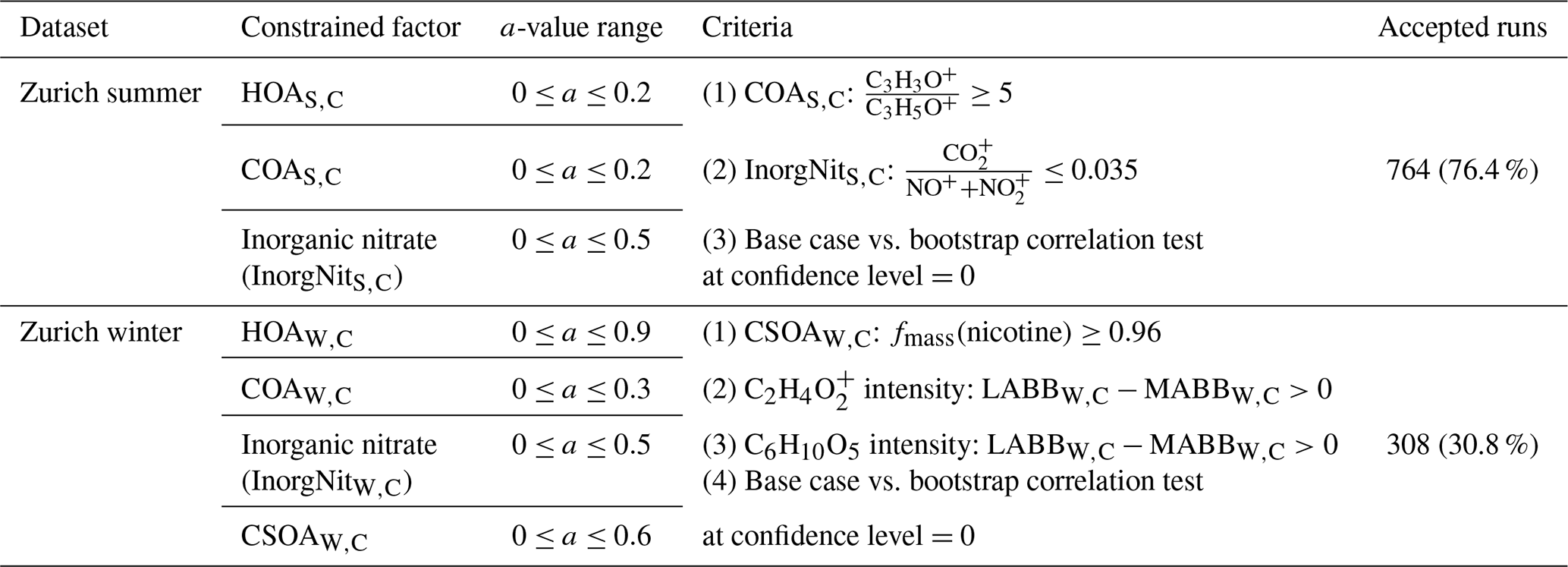
We have conducted cPMF analysis on datasets collected from the summer and winter campaigns. The parameters for the PMF analysis of the combined dataset and the re-analysed summer and winter datasets are summarised in Table 1. We re-ran the conventional PMF on the summer and the winter data, obtaining results similar to Stefenelli et al. (2019) and Qi et al. (2019), as discussed in Sect. S2. Other technical details of method validation and solution selections are also explained in the Supplement (from Sect. S2.2 to S2.4), including reference profile construction, the determination of CEESI and number of factors p, and the determination of a case-specific a-value range and acceptance criteria for bootstrap analysis. Table 2 summarises these case-specific facts for summer and winter datasets, including the a-value range for constrained factors, criteria for the a-value range and accepted bootstrap run selection, and the number of accepted runs from the final combined bootstrap.
Table 2Summary of a-value range for constrained factors, criteria for a value range and accepted bootstrap run selection, and the number of accepted runs from the final combined bootstrap and a-value analysis for the summer and winter datasets.
Here, we present final results from the cPMF analysis of the summer and winter campaigns in Sect. 3.1.1 and 3.1.2, respectively. The final solutions are reported as the average of all accepted bootstrap and a-value randomisation runs (764 for summer, 308 for winter), with uncertainties corresponding to the standard deviation. As the NO+ and NO signals are included in these two datasets and can result from either organic or inorganic nitrate, we estimate the organic and inorganic contributions to the NO+ and NO signal in each factor using the method of Kiendler-Scharr et al. (2016) (see Sect. S3). We compare the cPMF factors to their counterparts from the standalone AMS and EESI-TOF solutions for cases where a clear factor-to-factor correspondence exists. The further exploration on EESI-TOF sensitivities to resolved factors are discussed in Sect 3.2.
Due to the complexity of the analysed datasets (2 seasons ×3 PMF methods), we use the following convention for identifying factors: factorNameseason,method, where “factorName” is the name of the factor (e.g. COA for cooking-related organic aerosol), “season” denotes either the summer (“S”) or winter (“W”) dataset, and “method” refers to PMF on a standalone AMS dataset (“A”), standalone EESI-TOF dataset (“E”), or combined dataset (“C”). For example, COAS,C stands for the cooking-related factor retrieved from cPMF applied to the summer dataset.
3.1 cPMF results
3.1.1 cPMF analysis: Zurich summer
Eight factors were resolved from the Zurich summer campaign: HOAS,C, COAS,C, CSOAS,C, InorgNitS,C, two daytime SOA factors (DaySOA1S,C and DaySOA2S,C), and two nighttime SOA factors (NightSOA1S,C and NightSOA2S,C). The mean time series, diurnal cycles, and the mass spectra of these factors over 764 accepted runs are shown in Fig. 3, together with the time series from AMS-only PMF and/or EESI-TOF-only PMF when the corresponding standalone factor(s) exist. An estimate of campaign-average percent uncertainty in the mass concentration of each factor, calculated as the median of the standard deviation across all accepted runs, is given in Table S2. Many factor characteristics from cPMF resemble those previously discussed in detail for single-instrument AMS PMF and/or EESI-TOF PMF (Stefenelli et al., 2019). Therefore, only a summary discussion of these characteristics is presented here, and we focus on new information and/or differences obtained by the cPMF analysis. Recall that factor profiles for HOAS,C, COAS,C, and InorgNitS,C are constrained as discussed above.

Figure 3Mean factor time series (a), diurnal cycles (b), and factor profiles (c) from the 764 accepted bootstrap runs from cPMF analysis. In panel (a), the average factor time series are shown in red, and corresponding AMS and/or EESI-TOF factors from standalone PMF are shown in green and blue, respectively. Shaded areas represent the standard deviation across all accepted runs and are summarised in Table S2. In panel (b), the average diurnal cycles are displayed as solid red lines. Shaded areas denote the standard deviation over the average diurnal from individual solutions over all 764 accepted runs. Dashed lines denote the maximum and minimum mean diurnal observed within these 764 runs. For comparison, the AMS and EESI-TOF PMF factor time series and diurnal cycles from the individual dataset in Stefenelli et al. (2019) are shown in green and blue, respectively, for related factors. In panel (c), the average factor profiles are coloured by different ion families. Here, the AMS factor profiles are in the unit of µg m−3 (each factor sums to 1 µg m−3), whereas the EESI-TOF spectra are in the unit of cps (each factor sums to the total signal derived from 1 µg m−3 of the factor). Note that the NO+ and NO signal is divided into inorganic and organic contributions.
HOAS,C. The AMS mass spectrum is dominated by the CnH, and CnH series, consistent with n-alkanes and branched alkanes (Zhang et al., 2005; Lanz et al., 2007; Ulbrich et al., 2009; Ng et al., 2011a; Qi et al., 2019; Stefenelli et al., 2019). The diurnal cycle of HOAS,C has three clear peaks (see Fig. 3b); however, compared to HOAS,A from Stefenelli et al. (2019), their intensities are weaker. Specifically, the morning peak intensity ratio to the evening peak intensity is almost 1 in the HOAS,A factor, whereas in HOAS,C, the morning peak is ∼ one-third of the evening peak. In terms of contribution to total OAs, the HOAS,A factor contributes 5.8 % (0.177 µg m−3) of the total OAs, whereas in the cPMF analysis, this factor only contributes 3.1 % (0.092 µg m−3) of the total OAs.
COAS,C. This factor is characterised by long-chain fatty acids and alcohols, e.g. coronaric acid and/or its isomers at 319.2 ([C18H32O3]Na+), oleic acid and/or its isomers at 305.2 ([C18H34O2]Na+), and 2-oxo-tetradecanoic acid and/or its isomers at 293.2 ([C16H30O3]Na+). Similar to previous work, the AMS profile shows both alkyl fragments and slightly oxygenated ions, consistent with aliphatic acids from cooking oils (Hu et al., 2016). The AMS profile is characterised by a high ratio of C3H3O+ to C3H5O+ (∼5 here), slightly higher than in other studies (Sun et al., 2016a, b; Xu et al., 2019; Zhao et al., 2019), as well as high contributions from C5H8O+, C6H10O+, and C7H12O+. Both cPMF and single-instrument PMF analyses yield peaks during lunch (∼ 11:30 to 13:30 local time, UTC+2) and dinner (∼ 18:30 to 20:30 local time, UTC+2). The time series of COAS,C is strongly correlated with those of the single-instrument solutions, with Pearson's r2 of 0.846 and 0.634 against COAS,A and COAS,E, respectively.
CSOAS,C. The EESI-TOF factor profile is dominated by nicotine (detected as [C10H13N2]H+) at 163.12 and levoglucosan at 185.042 ([C6H10O5]Na+), which derives from pyrolysis of the cellulose present in tobacco (Talhout et al., 2006). In the AMS profile, this factor accounts for 79.3 % of the signal from C5H10N+ at 84.081, which is attributed to a fragment of n-methyl pyrrolidine and was previously identified as a tracer for cigarette smoke (Struckmeier et al., 2016). The time series of CSOAS,C correlates with that of the AMS-only and EESI-TOF solutions, with r2 of 0.922 and 0.965, respectively. The diurnal cycles from the combined- and single-instrument solutions are likewise correlated, showing high concentrations at night and low concentration during daytime.
InorgNitS,C. Among the accepted bootstrap runs, the mean ratio is 0.0346, slightly higher than the ratio of 0.0345 observed during the NH4NO3 calibration period, probably due to (1) uncertainties in the constrained profile and/or (2) a small amount of OA apportioned to this factor. The time series of this factor correlates with AMS nitrate (NO), NO+, and NO time series, with r2 of 0.654, 0.645, and 0.956, respectively. Regarding the mass fraction, approximately 48.5 % of the NO+ signal and 78.0 % of the NO signal are apportioned to this factor, followed by the two NightSOAS,C factors. This is consistent with the overall NO+ and NO signals deriving not only from inorganic nitrate but also from organonitrates (in other factors).
DaySOA1S,C and DaySOA2S,C. The cPMF analysis yields two SOA factors that are elevated during daytime, denoted DaySOA1S,C and DaySOA2S,C. The EESI-TOF spectra are similar to two factors retrieved from EESI-TOF-only PMF analysis by Stefenelli et al. (2019) but were not resolved in AMS-only PMF, where only more- and less-oxygenated SOA factors (MO-OOAS,A and LO-OOAS,A) were obtained. These factors contain strong signatures from terpene oxidation products, e.g. monoterpene-derived ions (C10H16Ox, x=5, 6, 7) and sesquiterpene oxidation products (C15H24Ox, x=3, 4, 5). A detailed comparison of the two DaySOA factors from the cPMF analysis to the LO-OOAS,A and MO-OOAS,A factors from AMS-only PMF is shown in Fig. S31 in the Supplement, and a comparison between the two DaySOAS,C factors and DaySOAS,E factors is shown in Fig. S32a and b, respectively. The AMS ions in these two factors are characterised by a strong CO signal, similar to the LO-OOAS,A and MO-OOAS,A factors, indicating that they largely consist of oxygenated OA, consistent with the EESI-TOF spectra. We calculate fracON for DaySOA1S,C and DaySOA2S,C to be 0.869 and 1.000, respectively, demonstrating that the NO+ and NO signal in these factors is dominated by organonitrates. Regarding the time series, DaySOA1S,C and DaySOA2S,C correlate strongly with DaySOA1S,E and DaySOA2S,E, with r2 of 0.883 and 0.977, respectively. The diurnal patterns of DaySOA1S,C and DaySOA2S,C are consistent with the diurnal patterns of DaySOA1S,E and DaySOA2S,E. The diurnal patterns of both factors show an enhancement in the afternoon and the evening, which distinguishes these SOAs from other SOAs: DaySOA1S,C exhibits almost a factor of 2 enhancement in signal between 15:00 and 21:00 compared to the morning, whereas the DaySOA2S,C exhibits the same magnitude of enhancement in signal around 12:00 to 17:00.
NightSOA1S,C and NightSOA2S,C. We retrieve two SOA factors that are enhanced overnight and in the early morning, denoted NightSOA1S,C and NightSOA2S,C. Their factor profiles and time series and/or diurnals closely resemble those of NightSOA1S,E and NightSOA2S,E (see Fig. S32c and d). Similar to the DaySOAS,C factors, terpene oxidation products are evident. However, the composition is weighted towards less-oxygenated and more-volatile terpene oxidation products, e.g. C10H16O2 and C10H16O3, which likely partition to the particle phase at night when temperature decreases. In addition, signals consistent with monoterpene-derived organonitrates are also evident, e.g. the C10H17O6−8N and C10H15O6−9N series, which are consistent with nighttime oxidation of monoterpenes by NO3 radicals (Xu et al., 2015; Faxon et al., 2018; Zhang et al., 2018). The AMS ions in these two factors are characterised by a strong CO signal and also a relatively high NO+ signal compared to ΣDaySOAsS,C. The ratio of is 4.55 and 8.24 for NightSOA1S,C and NightSOA2S,C, respectively, yielding fracON for NightSOA1S,C and NightSOA2S,C of 0.798 and 1, indicating high organonitrate content. These two factors correlate well with ΣNightSOAsS,E, reaching r2 of 0.975 and 0.897, generally following the same diurnal patterns, with NightSOA1S,C peaking from 22:00 to 05:00 local time, UTC+2 and NightSOA1S,C peaking from 04:00 to 12:00 local time, UTC+2.
3.1.2 cPMF analysis: Zurich winter
Twelve factors were resolved from cPMF analysis of the Zurich winter campaign: HOAW,C, COAW,C, InorgNitW,C, CSOAW,C, SOA1W,C, SOA2W,C, a more-aged biomass-burning OA (MABBW,C), two less-aged biomass-burning OAs (LABB1W,C and LABB2W,C), two nitrogen-containing OA factors (NitOA1W,C and NitOA2W,C), and a factor related to a specific local event (EVENTW,C). Because no significant chemical differences are apparent between LABB1W,C and LABB2W,C (see Figs. S33 and S34), they are aggregated to a single LABBW,C factor for presentation. Therefore, there are 11 factors presented below. The average time series and mass spectra of these factors among 308 accepted runs are shown in Fig. 4. The factor profiles for HOAW,C, COAW,C, InorgNitW,C, and CSOAW,C are constrained as described previously. Similar to the summer dataset, uncertainties in the factor mass concentrations are summarised in Table S2.
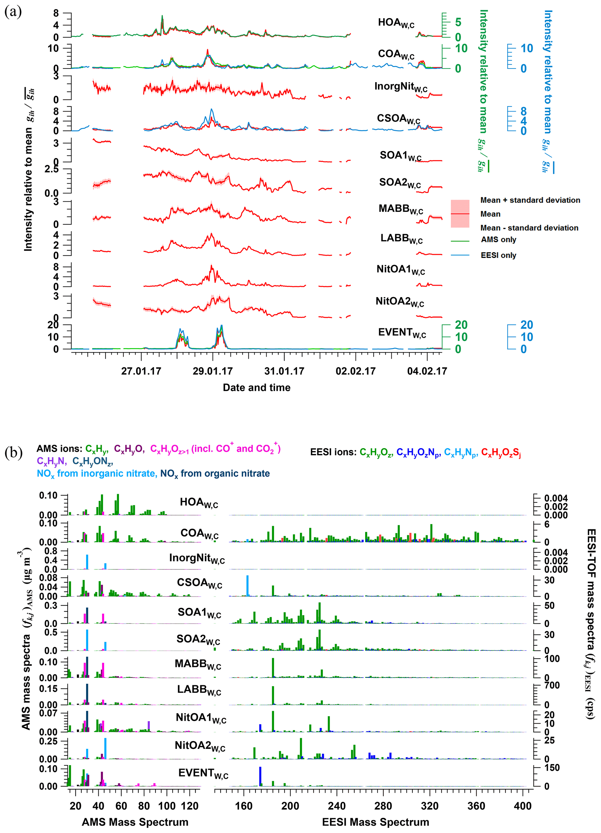
Figure 4Average factor time series (a) and factor profiles (b), which are calculated as the mean of all accepted bootstrap runs (308 runs in total). In panel (a), the average factor time series are shown in red, and corresponding AMS and/or EESI-TOF factors from standalone PMF are shown in green and blue, respectively. Shaded areas represent the standard deviation across all accepted runs and are summarised in Table S2. In panel (b), the average factor profiles are coloured by different ion families. Here, the AMS factor profiles are in the unit of µg m−3 (each factor sums to 1 µg m−3), whereas the EESI-TOF spectra are in the unit of cps (each factor sums to total signal derived from 1 µg m−3 of the factor). Note that the NO+ and NO signals are divided into inorganic and organic contributions.
HOAW,C. This factor is dominated by the CnH and CnH series, consistent with n alkanes and branched alkanes, with lower CO+ and CO content than the HOAS,C. The HOAW,C time series correlates strongly with HOAW,A (r2 of 0.913).
COAW,C. The COAW,C profile is characterised by long-chain fatty acids and alcohols, e.g. coronaric acid and/or its isomers at 319.2 ([C18H32O3]Na+), oleic acid and/or its isomers at 305.2 ([C18H34O2]Na+), and 2-oxo-tetredecanoic acid and/or its isomers at 293.2 ([C16H30O3]Na+), and in the AMS, a combination of alkyl fragments and slightly oxygenated ions from aliphatic acids from cooking oils, including C5H8O+, C6H10O+, and C7H12O+. These are key features of the constrained reference profile () (Qi et al., 2019) and COA factors found in other studies (Stefenelli et al., 2019; Tong et al., 2021). The COAW,C time series correlates with the corresponding single-instrument analyses, exhibiting r2 of 0.894 and 0.798 with COAW,A and COAW,E, respectively.
InorgNitW,C. As noted in Sect. S2.2, the ratio of this factor (2.42) is higher than that of pure NH4NO3 measured on site (1.58), consistent with the presence of other inorganic nitrate sources such as KNO3. Also, the mean ratio is 0.0371, higher than the ratio of 0.0261 from the constructed InorgNitW,C profile, which is probably due to (1) uncertainties in the constrained profile and/or (2) a small amount of OA apportioned to this factor. The time series of this factor shows high correlations with the AMS nitrate (NO), NO+, and NO time series, with r2 of 0.739, 0.792, and 0.754, respectively. Regarding the mass fraction, only 13.7 % of the NO+ signal and 13.2 % of the NO signal are apportioned to this factor. The considerable fractions of the NO+ and NO signals from inorganic nitrate and organonitrates in other factors are estimated as discussed above (Kiendler-Scharr et al., 2016) and will be interpreted later for the relevant factors (as summarised in Table S1).
CSOAW,C. Similar to CSOAS,C, nicotine at 163.12 and levoglucosan at 185.042 were found to be the two highest peaks in the EESI-TOF mass spectra, contributing 8.75 % and 4.56 % of the EESI-TOF signal. The time series of this factor resolved from cPMF analysis correlates with CSOAW,E (r2=0.662). Similar to CSOAW,C, the fragment of cigarette smoke tracer n-methyl pyrrolidine C5H10N+ at 84.081 is also found here. This is a minor factor, comprising 2.4 % of OAs.
SOA1W,C and SOA2W,C. These two factors have different temporal patterns. SOA1W,C decreased gradually from 26 to 30 January, whereas SOA2W,C increased from 26 January, fluctuated at high levels from 28 to 31 January, and then decreased from 1 February on. From the AMS perspective, both factors are characterised by high NO+, NO, and CO signals compared to other organic ions. Organonitrates account for all NO+ and NO signals in SOA1W,C but contribute nothing in SOA2W,C. Aside from the NO+ and NO ions, these AMS spectra are similar to the profiles of MO-OOAW,A and LO-OOAW,A, which are characterised by high CO signals. Major ions in the EESI-TOF profile include C10H16Ox (x=3, 4, 5), C9H14Ox (x=3, 4), C8H12Ox (x=4, 5), C10H18O4, and C10H14O5, which are also found in secondary biomass burning (three MABBW,E factors) and/or terpene oxidation factors (SOA1W,E and SOA2W,E) from Qi et al. (2019). However, the H:C ratio of these two factors from the EESI-TOF component (1.578 and 1.588 for SOA1W,C and SOA2W,C, respectively) is less than that of DaySOA1S,C (1.650) and DaySOA2S,C (1.672), suggesting an increased contribution from aromatic precursors.
Biomass-burning factors (LABBW,C and MABBW,C). We resolve a less-aged biomass-burning factor (LABBW,C, which, as mentioned above, is the aggregate of two similar LABB factors) and a more-aged biomass-burning factor (MABBW,C). Consistent with Qi et al. (2019), the EESI-TOF component of LABBW,C is characterised by a large signal from [C6H10O5]Na+ (mainly levoglucosan) (20.4 %), and MABBW,C by a smaller but notably non-zero one (6.21 %). In addition, 76.7 % and 11.9 % of the total levoglucosan signal is apportioned to LABBW,C and MABBW,C, respectively. The difference in the fraction of total levoglucosan apportioned to these two factors suggests different degrees of ageing of biomass-burning-emitted OAs. The AMS spectrum of the BBOAW,A factor is characterised by C2H4O and C3H5O, which are typical fragments of anhydrosugars, such as levoglucosan (Alfarra et al., 2007; Lanz et al., 2007; Sun et al., 2011). These ions are also present in LABBW,C and MABBW,C and are higher in LABBW,C (1.91 % vs. 0.879 % for C2H4O and 0.978 % vs. 0.323 % for C3H5O). In addition, the ratio of C2H4O to CO is 0.396 and 0.092 for LABBW,C and MABBW,C, respectively, supporting the separation of these factors based on different degrees of ageing.
EVENTW,C. This factor is low throughout the campaign, except for the nights of 28 and 29 January from 00:00 to 07:00 UTC+2, where large peaks are observed. Therefore, it likely corresponds to a specific event near the sampling location. The mass spectrum features ions at 174.08, 185.04, and 195.06, tentatively assigned to [C8H11N2O]Na+, [C6H10O5]Na+, and [C8H12O4]Na+ from the EESI-TOF part and at 15.024 (CH), 27.027 (C2H), 31.018 (CH3O+), and 43.018 (C2H3O+) from the AMS part. Qi et al. (2019) observed a very similar factor in standalone EESI-TOF PMF, which was tentatively attributed to the Zurich gaming festival and/or plastic burning in a nearby restaurant. The factor includes large contributions from C8H12O4, which likely represents 1,2-cyclohexane dicarboxylic acid diisononyl ester, a plasticiser for the manufacture of food packaging. In the AMS spectrum, large signals from NO+ (7.36 %) and NO (2.03 %) are also observed, with 46.6 % of the NO+ signal and 23.6 % of the NO signal assigned to organonitrates. Similar to Qi et al. (2019), the AMS spectrum is also dominated by the ions in the CxHyO group.
NitOA1W,C. This factor is characterised by a high signal of C5H10N+ at 84.081, contributing 4.02 % to the AMS intensity in this factor (no other factor exceeds 0.16 %), while 97.0 % of the C5H10N+ mass is apportioned to this factor. This ion is considered to be a tracer of cigarette smoking (Struckmeier et al., 2016); however, different from typical CSOA mass spectra, this factor also has high signal from CO, suggesting a contribution from secondary formation processes. Similar to other OA factors, this factor also has a considerable fraction of NO+ and NO signals, attributed entirely to organonitrates. For the EESI-TOF component, this factor is characterised by [C8H11N2O]Na+, levoglucosan and [C8H11N2O]Na+, [C6H10O5]Na+, [C9H12O4]Na+, and [C11H14O4]Na+, suggesting this factor may also be influenced by fresh biomass burning.
NitOA2W,C. This factor is characterised by a high fraction of total signals from the CHON group in the EESI-TOF analysis (38.5 %). Among these ions, [C7H11O6N]Na+ at 228.048, [C10H15O6N]Na+ at 268.079, and [C10H17O7N]Na+ at 286.090 are the three highest ions, contributing 1.65 %, 1,99 %, and 1.98 %, respectively. There are also some typical ions with high intensity from biomass-burning ageing (Qi et al., 2019; Stefenelli et al., 2019), e.g. [C9H14O4]Na+ at 209.078, [C10H14O6]Na+ at 253.068, and [C10H16O6]Na+ at 255.084, contributing 6.47 %, 2.85 %, and 4.39 %, respectively. This may suggest a contribution from biomass-burning activities. From the AMS perspective, this factor is characterised by high NO+ and NO signals, in which all of the NO+ and NO signals are produced from inorganic nitrates (see Table S1), with the other ions being qualitatively similar to OOA-type spectra.
3.2 EESI-TOF sensitivity to resolved factors
AMS and EESI-TOF contributions to the factor profiles are intrinsically linked by cPMF. That is, for each individual factor, the two instrument profiles by definition describe the same OA fraction. Therefore, the EESI-TOF sensitivity to a factor ASk can be calculated according to Eq. (10). Note that this calculation depends on the following assumptions: (1) both instruments are well-represented in the solution; (2) the PMF solution is of high quality (i.e. factors are all meaningful and well-separated, without significant mixing or splitting); (3) solution uncertainties are not so high as to preclude quantitative interpretation of the results. Assumption (1) was discussed earlier in the context of instrument weighting, and assumption (2) is supported by the interpretability of the factors, as presented in the previous section. By performing the cPMF analysis on a large number of runs combining bootstrap analysis and a-value exploration, we can estimate uncertainties in the calculated sensitivities imposed by the analysis model, as presented below, thereby addressing assumptions (2) and (3).
The datasets analysed here were taken from the first field deployments of the EESI-TOF. As a result, operational protocols were not yet fully standardised across campaigns. Specifically, we lack reliable on-site calibration with a chemical standard common to the two campaigns (this was attempted, but the measurements were evaluated to be unreliable during post-analysis due to operational problems). Therefore, to enable comparison of relative factor sensitivities between the summer and winter campaigns, we select COA as a reference. That is, we assume . We choose COA, because it is the only factor that both (1) appears in all four single-instrument datasets (i.e. summer and winter, AMS and EESI-TOF) and (2) compared to other factors, is less likely to significantly change in composition between the campaigns (in contrast to, e.g. SOAs in Zurich, which are known to have significantly different precursors in summer and winter). Therefore, all sensitivities below are reported as (), in which ASk is calculated in every bootstrap run and then referenced to (the mean ASCOA calculated over all bootstrap runs). Here, k denotes a given factor from the (summer or winter) cPMF solutions. Note that EESI-TOF sensitivities to HOA and InorgNit are not discussed here, since they are undetectable by the EESI-TOF (as configured for these campaigns; see Sect. 2.2.2) and therefore constrained to be ∼0.01 cps (µg m−3)−1. The mean and standard deviation of factor-dependent for the summer and winter datasets are shown in Fig. 5, with histograms summarising all accepted runs shown in Figs. S35 and S36. For ease of viewing, the factors in Fig. 5 are collected into related groups. We also calculate the ASk's for several factor aggregations. First, five factors that are likely related to biomass burning (LABBW,C, MABBW,C, NitOA1W,C, NitOA2W,C, and EVENTW,C) are denoted as the “ΣBB” factor. Additionally, we separately aggregate the two DaySOAS,C and two NightSOAS,C factors, denoted “ΣDaySOAsS,C” and “ΣNightSOAsS,C”, respectively. As seen in Fig. 5 (as well as in Figs. S35 and S36 and Table S3), the relative uncertainty from the summer factors is systematically lower than for the winter factors within the accepted solutions. This may indicate higher source apportionment quality and solution stability for the former but is also related to the sub-division of factors related to primary biomass-burning-related factors, as discussed later.
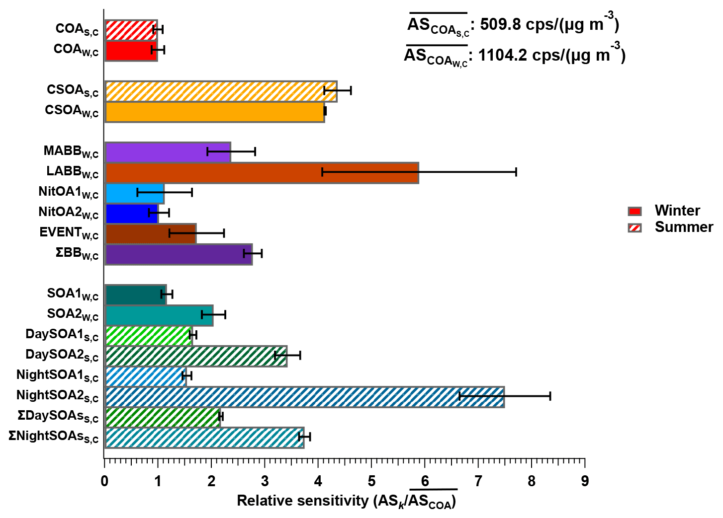
Figure 5Comparison of of different factors resolved from the cPMF on the summer and winter datasets. Mean values are shown as bars, and error bars indicate the standard deviation over all accepted bootstrap runs. The following factor aggregations are also shown: ; ; and .
For COAS,C and COAW,C, the mean relative sensitivities are 1 by definition, though uncertainties are still calculated due to non-zero a values, while the reference profile utilised for CSOAW,C ensures that CSOAW,C and CSOAS,C will have similar sensitivities. Interestingly, the distribution of the sensitivities of COAS,C, COAW,C, and CSOAW,C in Figs. S32 and S33 is clearly multi-modal despite a-value constraints (although the overall COAS,C and COAW,C distributions remain relatively narrow), but the reason for this is unknown.
The next group of factors (LABBW,C, MABBW,C, NitOA1W,C, NitOA2W,C, and EVENTW,C) includes non-negligible contributions from levoglucosan (C6H10O5), produced typically from biomass-burning (BB)-related activities. Previous work has demonstrated that the EESI-TOF sensitivity to levoglucosan is higher than that of many other compounds and bulk SOA from representative precursors (Lopez-Hilfiker et al., 2019; Brown et al., 2021). Indeed, although the set of studied compounds is far from comprehensive, the relative sensitivity of the EESI-TOF to levoglucosan is among the highest yet recorded. Therefore, despite the variation in composition of the POA-influenced factors, the effect of the C6H10O5 content on the overall factor sensitivity is often considerable for cases where this ion is strongly influenced by levoglucosan. Figure 6 shows ASk as a function of the C6H10O5 fraction for all factors for which the C6H10O5 signal is believed to result largely from levoglucosan. This analysis accounts for all factors resolved from the cPMF of the winter dataset, except for CSOAW,C, because CSOAW,C is dominated by the signal from the protonated nicotine ([C10H14N2]H+) ion, which is both chemically different (reduced nitrogen) and has a different ionisation pathway than other measured ions. The four summer SOA factors are excluded as well, because the contribution from C6H10O5 in these factors was previously attributed to terpene and/or aromatic oxidation products (Stefenelli et al., 2019). An obvious qualitative trend of increasing sensitivity with increasing levoglucosan fraction is evident, with Pearson r2 of 0.676, indicating the overwhelming influence of the high-sensitivity species levoglucosan on the factor-apparent sensitivity.
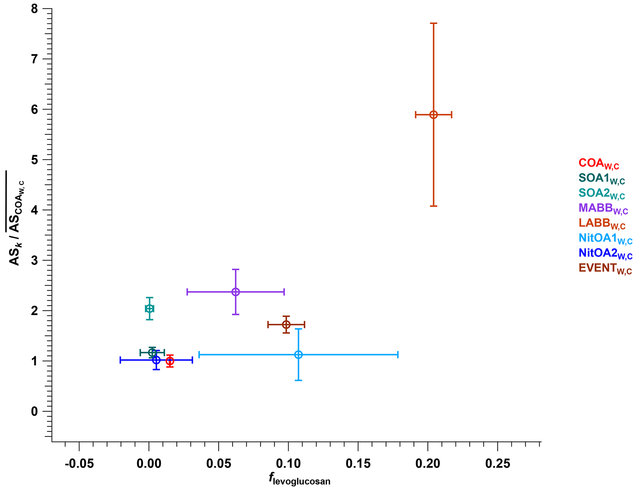
Figure 6Relative apparent sensitivity as a function of levoglucosan fraction for all factors resolved from the cPMF of the winter dataset, except for CSOAW,C. Error bars denote standard deviation.
For the primary BB-related factors, the uncertainties are generally higher than for the other factors (see Fig. S36). In contrast, the aggregated BB factor (ΣBBW,C and ) is less uncertain and has a narrower sensitivity distribution. This suggests that the overall classification of signal as biomass-burning related is robust, but the subdivision into more specific BB-related sources carries higher uncertainties. Likewise, the relative sensitivities of ΣDaySOAsS,C and ΣNightSOAsS,C are less uncertain compared to individual corresponding SOA factors in summer (as shown in Fig. S35). This contrast suggests that coarse classifications of factors may have higher precision but may provide less information, whereas fine classifications of factors may have higher uncertainties but may potentially provide more information from each factor. It also suggests that, at least for these datasets, factor mixing occurs primarily between factors with closely related sources. Despite their higher uncertainties, the finest classification levels explored here still appear to be meaningful. We also note that both datasets investigated here are of relatively short duration, and factor separation may improve in longer datasets.
The final group of factors in Fig. 5 corresponds to SOAs. The relative sensitivities of the SOA factors in winter are shown to be lower than any of the SOA factors resolved during summer. This is consistent with expectations regarding the seasonal differences in the dominant SOA precursors and the expected ASk of the resulting SOAs. At this site, SOA precursors are expected to be dominated by monoterpenes in summer and by biomass burning (increasing the contribution of phenols, naphthalenes, and other aromatics) in winter, with traffic making a lesser contribution in both seasons (Daellenbach et al., 2016; Qi et al., 2020). This is supported by analysis of the characteristics of the retrieved factors, as discussed above (Qi et al., 2019; Stefenelli et al., 2019). Previous studies have shown differences in the EESI-TOF bulk sensitivity to SOAs from different precursors, with terpene-derived SOAs generally exhibiting higher sensitivity than SOAs from light aromatics (Lopez-Hilfiker et al., 2019; Wang et al., 2021). Figure 7 shows the for two DaySOAS,C and NightSOAS,C factors in summer, as well as the ΣDaySOAsS,C and ΣNightSOAsS,C – which are the aggregates of the individual DaySOAS,C and NightSOAS,C factors (ΣDaySOAs and ), respectively – and two SOAW,C factors in winter as a function of their H:C ratio calculated from the EESI-TOF component. A trend of increasing sensitivity with increasing H:C ratio is observed for the summer SOAs and winter SOAs (SOA1W,C and SOA2W,C), with an overall Spearman's rank correlation of 0.833. Consistent with Wang et al. (2021), H:C is found to be a better predictor of ASk than either O:C or OSc, yielding Spearman's rank correlation of 0.833 for ASk vs. H:C, −0.167 for ASk vs. O:C, and −0.452 for ASk vs. OSc (Fig. S37a and b).

Figure 7 of SOA factors retrieved from the summer and winter datasets as a function of the H:C ratio. Error bars denote standard deviation across all accepted runs. Spearman correlation is 0.833, as indicated in the top-left corner.
For the SOA factors, we compare ASk retrieved to ASk predicted using a molecular formula-based parameterisation trained with laboratory SOA measurements, as described in Sect. 2.2.3 (Wang et al., 2021). No parameterisations presently exist for POA factors, so these are excluded from the comparison, although to allow comparison between campaigns, the model is used to calculate a reference value for ASCOA. Figure 8 compares the ASk values based on model predictions against values determined from cPMF. For summer SOAs, the LMN (limonene)-based parameterisation is applied as a surrogate for terpene oxidation products. Regarding the winter SOAs, three scenarios (cresol, LMN, and TMB) are applied, as the winter SOAs in Zurich are mainly related to oxidation of biomass-burning emissions, which include monoterpenes, phenols, naphthalenes, and other aromatics (Rouvière et al., 2006; Bruns et al., 2016; Kelly et al., 2018). In Fig. 8, 1:1, 1:2, 1:4, and 1:8 lines are provided to guide the eye, although a 1:1 correspondence is not expected, because the models are not trained on primary COAs. The figure shows a monotonic increase in model sensitivity predictions with increasing cPMF-derived sensitivities, with the sole exception of SOA2W,C. Specifically, the summer-derived points fall mainly between the 1:1 and 1:2 lines, while for SOA1W,C, the model predictions are roughly a factor of 2 lower relative to the cPMF results. This offset may reflect differences in the appropriateness of the selected precursor surrogate. The SOA2W,C factor is a slight outlier, probably because the ASk for this factor is more uncertain than the others (and not fully captured by the error bars in Fig. 5) due to the high contribution from inorganic nitrate (∼80 % of mass) in its factor profile. Given the limitations of the multi-variate parameterisation (see Sect. 2.2.3) and the several-orders-of-magnitude variation in EESI-TOF sensitivities to individual compounds, the qualitative agreement between ASk values independently retrieved from multivariate parameterisation and cPMF provide support for both methods.
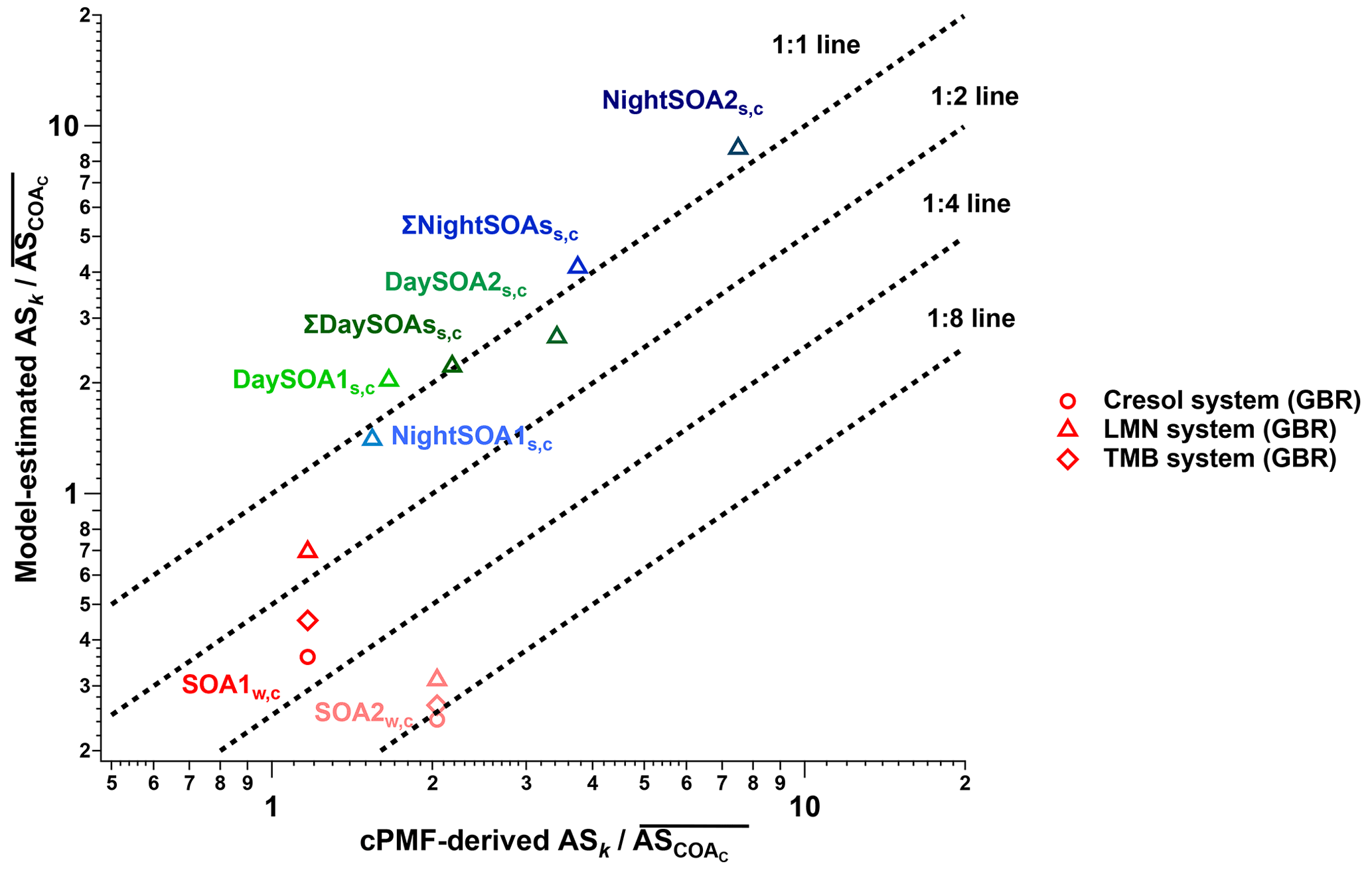
Figure 8The estimated relative apparent sensitivity to COAs () from the gradient-boosting regression (GBR) model as a function of cPMF-derived relative apparent sensitivity to COA (). The symbols indicate the different oxidation precursor systems (LMN for SOAs produced from oxidation of limonene by ozone, cresol and TMB for SOAs produced from oxidation of o-cresol and 1,3,5-trimethylbenzene by OH radicals, respectively).
The application of factor-dependent sensitivities can qualitatively and quantitatively affect the source apportionment results. Figure 9a and b compare the source apportionment results from cPMF on the summer and winter datasets using the calculated factor sensitivities (ASk) (i.e. direct outputs of the cPMF analysis) vs. using a single bulk sensitivity (ASbulk) for all factors, where the latter is calculated as the ratio of the total OA measured by the EESI-TOF (cps) to that measured by the AMS (µg m−3). Figure 10a and b compare the total OA concentrations returned from the cPMF using ASk and ASbulk to the total OA measured by the AMS. Table S3 summarises the retrieved ASk values for each factor (note that, although the relative ASk are believed to be intrinsic properties of the factors, the absolute sensitivities are instrument- and tuning-dependent and will vary between campaigns).
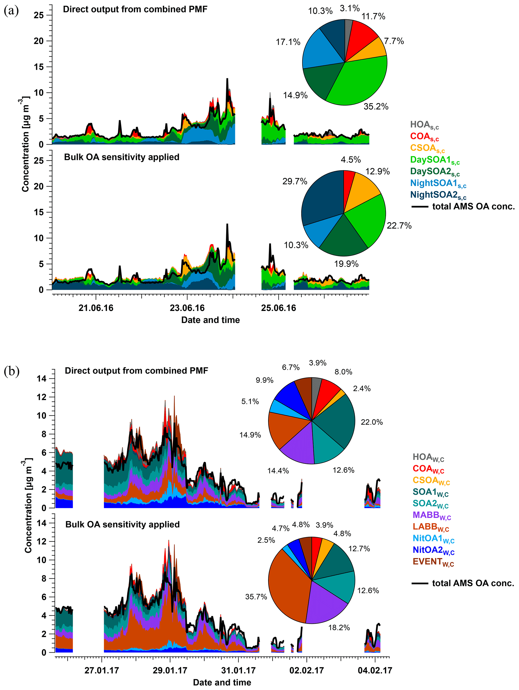
Figure 9Comparison of source apportionment results between direct output from cPMF (i.e. accounting for factor-dependent sensitivities) and application of a single bulk OA sensitivity, applied to the Zurich summer (a) and winter (b) datasets. Stack plots of factor time series directly from combined PMF and factor time series calculated from bulk OA sensitivity compared with total AMS OA concentration are shown in the upper and lower panel, respectively, in each subfigure, together with the corresponding factor contribution shown in the pie chart. Note that, here, the contribution of the InorgNit factor and the contributions of NO+ and NO from inorganic nitrate in each factor are excluded to account only for the total OA.

Figure 10Comparison between the sum of factor concentrations in each time point with (in red) and without (in blue) taking the factor-dependent sensitivity into account and total OA measured by AMS for summer in panel (a) and winter in panel (b). A linear fit is conducted based on the Levenberg–Marquardt least-orthogonal-distance method. Note that, here, the contribution of the InorgNit factor and the contributions of NO+ and NO from inorganic nitrate in each factor are excluded.
In the Zurich summer campaign, the bulk OA sensitivity (1254.0 cps (µg m−3)−1) is higher than that of (509.8 cps (µg m−3)−1). Four factors (HOAS,C, COAS,C, DaySOA1S,C, and NightSOA1S,C) are underestimated, whereas three factors (CSOAS,C, DaySOA2S,C, and NightSOA2S,C) are overestimated when is used. Using the calculated ASk, the contribution of COAS,C to total OA more than doubles from 4.5 % to 11.7 %, as shown in Fig. 9a. Similarly, the application of ASk increases the contributions of DaySOA1S,C and NightSOA1S,C from 22.7 % to 35.2 % and from 10.3 % to 17.1 %, respectively. Among the overestimated factors, the largest decrease post-correction is found for NightSOA2S,C, the contribution of which decreases by approximately a factor of 3 (from 29.7 % to 10.3 %). Smaller post-correction decreases are observed for the contributions of CSOAS,C (12.9 % to 7.7 %) and DaySOA2S,C (19.9 % to 14.9 %). If factor-dependent sensitivities were ignored, NightSOA2S,C would be the largest contributor to total OA, followed by DaySOA1S,C, whereas the full analysis indicates that DaySOA1S,C is the largest contributor.
Similar to the summer campaign, application of ASk significantly affects the source apportionment results in winter. CSOAW,C, MABBW,C, and LABBW,C are shown to be overestimated, while HOAW,C, COAW,C, SOA1W,C, NitOA1W,C, NitOA2W,C, and EVENTW,C are underestimated. If factor-dependent sensitivities were not considered, LABBW,C and MABBW,C would appear to be the dominant contributors to total OA (35.7 % and 18.2 %, respectively) due to their high levoglucosan content. However, the full cPMF analysis indicates the LABBW,C and MABBW,C contributions to be 14.9 % and 14.4 %, respectively, whereas accounting for ASk increases the contribution of SOA1W,C from 12.7 % to 22.0 %, making it the largest contributor.
For both the summer and winter datasets, calculation of total OA from cPMF results using factor-specific ASk significantly outperforms that using a single ASbulk. This is evident from an increased r2 (0.966 vs. 0.821) for summer. However, the r2 is similar between the two approaches in winter (0.947 vs. 0.943). The difference after applying ASk and ASbulk in r2 might be related to the extent to which the contribution from factors with high ASk and low ASk to total OA changes over time during the campaign, which can vary in different datasets.
Box-and-whisker diagrams of factor contributions to total OA with and without applying ASk values for summer and winter are presented in Fig. 11. In the Zurich summer campaign, the box plots of the corrected contributions of all six factors fall completely outside of the interquartile range (IQR) of the uncorrected results, suggesting that the use of a single ASbulk would lead to significant biases. In contrast, the winter campaign exhibits a lack of overlap between the ASk- and ASbulk-derived results for eight factors (HOAW,C, COAW,C, CSOAW,C, SOA1W,C, SOA2W,C, NitOA1W,C, NitOA2W,C, and EVENTW,C), whereas two factors overlap (SOA2W,C and MABBW,C). This may result from statistical uncertainties in bootstrap analysis coupled with a less robust division between certain factors, yielding a wide distribution, e.g. MABBW,C, and/or ASk values that are similar to ASbulk (2271.1 cps (µg m−3)−1), e.g. SOA2W,C (2253.2 cps (µg m−3)−1) and MABBW,C (2619.0 cps (µg m−3)−1).
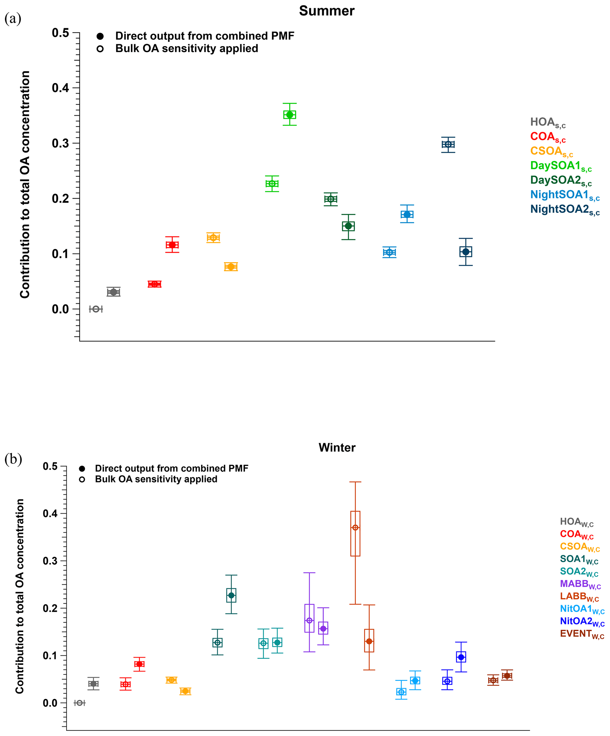
Figure 11Box-and-whisker diagrams of factor contributions to total OA with and without applying the factor dependent sensitivities for (a) summer and (b) winter within accepted solutions. For each pair of factors, the contribution without factor-dependent sensitivity applied is shown in the left box (open symbols), whereas the contribution corrected by factor-dependent sensitivity is shown in the right box (filled symbols). The box-and-whisker diagram shows the mean (open and filled circle), median (horizontal bar), interquartile range (rectangle, the 25th percentile is the lower edge, and the 75th is the upper edge), and minimum and maximum values (whiskers). Note that, here, the contribution of the InorgNit factor and the contributions of NO+ and NO from inorganic nitrate in each factor are excluded.
We address the longstanding challenges in achieving quantitative source apportionment of SOA sources by conducting a positive matrix factorisation (PMF) analysis of a dataset combining measurements from an aerosol mass spectrometer (AMS) and an extractive electrospray ionisation time-of-flight mass spectrometer (EESI-TOF). This approach combines the strengths of the two instruments – namely, the quantification ability of the AMS and the chemical resolution of the EESI-TOF. We demonstrate the utility of this approach by PMF analysis of combined EESI-TOF and AMS datasets collected during summer and winter in Zurich, Switzerland. The results retain the chemical resolution of the standalone EESI-TOF PMF while additionally providing quantitative factor time series and the EESI-TOF bulk sensitivity to different OA factors.
Note that, while these methods provide a general procedure for cPMF analysis, the specific parameters employed (i.e. the number of factors, p; instrument weighting parameter, Cinst; and the factors to be constrained and the tightness of constraints, a-value ranges) are dataset specific and should be determined independently for each new analysis.
The cPMF method intrinsically provides factor-dependent sensitivities (cps (µg m−3)−1) for the EESI-TOF. To account for organonitrate content, the AMS ions NO+ and NO are included in the cPMF analysis. Organic and inorganic contributions to these ions are estimated on a factor-by-factor basis using the method of Kiendler-Scharr et al. (2016).
For practical reasons, sensitivities between winter and summer campaigns are compared using cooking-related OA (COA) as a common reference. The retrieved factor sensitivities range from approximately 1.3 to 7.5 times the sensitivity of COA. The relative sensitivities of SOA factors are precursor dependent and are qualitatively consistent with trends observed in laboratory measurements of SOAs from single precursors (Lopez-Hilfiker et al., 2019). The SOA sensitivities estimated using our cPMF approach also agree with the sensitivities predicted by multi-variate regression models (Wang et al., 2021), which further demonstrates that SOA sensitivities are precursor and/or source dependent. Comparison of source apportionment results using factor-dependent sensitivities to uncorrected results show substantial differences, highlighting the importance of quantitative analysis. For example, before applying factor-dependent sensitivities, the contribution of a daytime SOA factor is underestimated by about 30 % (22.7 % before vs. 35.2 % after), whereas the contribution of a nighttime SOA factor is almost overestimated by a factor of 3 in the summer campaign (29.7 % before vs. 10.3 % after). As for the winter campaign, the contribution of a less-aged biomass-burning factor to total OAs in the Zurich winter dataset is 35.7 %, making it a major factor in winter without considering its factor-dependent sensitivity. However, this factor is significantly overestimated by more than a factor of 2 (35.7 %, before vs. 14.9 % after). In contrast, the SOA1 factor in winter is underestimated, with its contribution increasing from 12.7 % to 22.0 %.
These considerable differences in the source contributions between the uncorrected EESI-TOF and cPMF results highlight the challenges in interpreting standalone source apportionment results for instruments where ion-specific sensitivity information is not readily available, such as EESI-TOF or FIGAERO-CIMS. Although the time trends of such analyses are likely robust, interpretation of the relative composition requires caution. Therefore, if such interpretation is desired, it is advised to employ analysis strategies such as cPMF that are capable of integrating quantitative measurements from reference instruments.
The cPMF method presented herein can be utilised as is, not only for the AMS/EESI-TOF combination but for any dataset comprising data from multiple instruments. As such, it provides a promising strategy for utilising instruments with high chemical resolutions but semi-quantitative performance (i.e. a linear but hard-to-calibrate response to mass) within the framework of a quantitative source apportionment.
The data are available from the corresponding author upon request.
The supplement related to this article is available online at: https://doi.org/10.5194/amt-15-7265-2022-supplement.
GS and LQ conducted the campaigns in summer and winter in Zurich, respectively. YT performed the whole analysis. DSW performed the multi-variate model for machine learning parameterisation of sensitivities. FC developed the weighting and constraining functions in SoFi. JGS conceived and supervised the project. All authors currently working at PSI contributed to the data interpretation. All authors contributed to the manuscript revision.
The contact author has declared that none of the authors has any competing interests.
Publisher’s note: Copernicus Publications remains neutral with regard to jurisdictional claims in published maps and institutional affiliations.
We gratefully acknowledge the contribution from Anna Tobler and Gang Chen for coordinating the workstation for the computationally intensive bootstrap analysis.
This research has been supported by the Schweizerischer Nationalfonds zur Förderung der Wissenschaftlichen Forschung (grant no. BSSGI0_155846) and the H2020 Marie Skłodowska-Curie Actions (grant no. 701647).
This paper was edited by Glenn Wolfe and reviewed by Angela Buchholz and Michael Link.
Alfarra, M. R., Prevot, A. S. H., Szidat, S., Sandradewi, J., Weimer, S., Lanz, V. A., Schreiber, D., Mohr, M., and Baltensperger, U.: Identification of the mass spectral signature of organic aerosols from wood burning emissions, Environ. Sci. Technol., 41, 5770–5777, https://doi.org/10.1021/es062289b, 2007.
Allan, J. D., Jimenez, J. L., Williams, P. I., Alfarra, M. R., Bower, K. N., Jayne, J. T., Coe, H., and Worsnop, D. R.: Quantitative sampling using an Aerodyne aerosol mass spectrometer: 1. Techniques of data interpretation and error analysis, J. Geophys. Res.-Atmos., 108, 4090, https://doi.org/10.1029/2002JD002358, 2003.
Beelen, R., Raaschou-Nielsen, O., Stafoggia, M., Andersen, Z. J., Weinmayr, G., Hoffmann, B., Wolf, K., Samoli, E., Fischer, P., Nieuwenhuijsen, M., Vineis, P., Xun, W. W., Katsouyanni, K., Dimakopoulou, K., Oudin, A., Forsberg, B., Modig, L., Havulinna, A. S., Lanki, T., Turunen, A., Oftedal, B., Nystad, W., Nafstad, P., De Faire, U., Pedersen, N. L., Ostenson, C. G., Fratiglioni, L., Penell, J., Korek, M., Pershagen, G., Eriksen, K. T., Overvad, K., Ellermann, T., Eeftens, M., Peeters, P. H., Meliefste, K., Wang, M., Bueno-de-Mesquita, B., Sugiri, D., Kramer, U., Heinrich, J., de Hoogh, K., Key, T., Peters, A., Hampel, R., Concin, H., Nagel, G., Ineichen, A., Schaffner, E., Probst-Hensch, N., Kunzli, N., Schindler, C., Schikowski, T., Adam, M., Phuleria, H., Vilier, A., Clavel-Chapelon, F., Declercq, C., Grioni, S., Krogh, V., Tsai, M. Y., Ricceri, F., Sacerdote, C., Galassi, C., Migliore, E., Ranzi, A., Cesaroni, G., Badaloni, C., Forastiere, F., Tamayo, I., Amiano, P., Dorronsoro, M., Katsoulis, M., Trichopoulou, A., Brunekreef, B., and Hoek, G.: Effects of long-term exposure to air pollution on natural-cause mortality: an analysis of 22 European cohorts within the multicentre ESCAPE project, Lancet, 383, 785–795, https://doi.org/10.1016/S0140-6736(13)62158-3, 2014.
Bi, C., Krechmer, J. E., Frazier, G. O., Xu, W., Lambe, A. T., Claflin, M. S., Lerner, B. M., Jayne, J. T., Worsnop, D. R., Canagaratna, M. R., and Isaacman-VanWertz, G.: Quantification of isomer-resolved iodide chemical ionization mass spectrometry sensitivity and uncertainty using a voltage-scanning approach, Atmos. Meas. Tech., 14, 6835–6850, https://doi.org/10.5194/amt-14-6835-2021, 2021.
Brown, W. L., Day, D. A., Stark, H., Pagonis, D., Krechmer, J. E., Liu, X., Price, D. J., Katz, E. F., DeCarlo, P. F., Masoud, C. G., Wang, D. S., Hildebrandt Ruiz, L., Arata, C., Lunderberg, D. M., Goldstein, A. H., Farmer, D. K., Vance, M. E., and Jimenez, J. L.: Real-time organic aerosol chemical speciation in the indoor environment using extractive electrospray ionization mass spectrometry, Indoor Air, 31, 141–155, https://doi.org/10.1111/ina.12721, 2021.
Bruns, E. A., El Haddad, I., Slowik, J. G., Kilic, D., Klein, F., Baltensperger, U., and Prévôt, A. S. H.: Identification of significant precursor gases of secondary organic aerosols from residential wood combustion, Scientific Reports, 6, 27881, https://doi.org/10.1038/srep27881, 2016.
Canagaratna, M. R., Jayne, J. T., Jimenez, J. L., Allan, J. D., Alfarra, M. R., Zhang, Q., Onasch, T. B., Drewnick, F., Coe, H., Middlebrook, A., Delia, A., Williams, L. R., Trimborn, A. M., Northway, M. J., DeCarlo, P. F., Kolb, C. E., Davidovits, P., and Worsnop, D. R.: Chemical and microphysical characterization of ambient aerosols with the aerodyne aerosol mass spectrometer, Mass Spectrom. Rev., 26, 185–222, https://doi.org/10.1002/mas.20115, 2007.
Canonaco, F., Crippa, M., Slowik, J. G., Baltensperger, U., and Prévôt, A. S. H.: SoFi, an IGOR-based interface for the efficient use of the generalized multilinear engine (ME-2) for the source apportionment: ME-2 application to aerosol mass spectrometer data, Atmos. Meas. Tech., 6, 3649–3661, https://doi.org/10.5194/amt-6-3649-2013, 2013.
Canonaco, F., Tobler, A., Chen, G., Sosedova, Y., Slowik, J. G., Bozzetti, C., Daellenbach, K. R., El Haddad, I., Crippa, M., Huang, R.-J., Furger, M., Baltensperger, U., and Prévôt, A. S. H.: A new method for long-term source apportionment with time-dependent factor profiles and uncertainty assessment using SoFi Pro: application to 1 year of organic aerosol data, Atmos. Meas. Tech., 14, 923–943, https://doi.org/10.5194/amt-14-923-2021, 2021.
Chen, Y., Takeuchi, M., Nah, T., Xu, L., Canagaratna, M. R., Stark, H., Baumann, K., Canonaco, F., Prévôt, A. S. H., Huey, L. G., Weber, R. J., and Ng, N. L.: Chemical characterization of secondary organic aerosol at a rural site in the southeastern US: insights from simultaneous high-resolution time-of-flight aerosol mass spectrometer (HR-ToF-AMS) and FIGAERO chemical ionization mass spectrometer (CIMS) measurements, Atmos. Chem. Phys., 20, 8421–8440, https://doi.org/10.5194/acp-20-8421-2020, 2020.
Crippa, M., Canonaco, F., Slowik, J. G., El Haddad, I., DeCarlo, P. F., Mohr, C., Heringa, M. F., Chirico, R., Marchand, N., Temime-Roussel, B., Abidi, E., Poulain, L., Wiedensohler, A., Baltensperger, U., and Prévôt, A. S. H.: Primary and secondary organic aerosol origin by combined gas-particle phase source apportionment, Atmos. Chem. Phys., 13, 8411–8426, https://doi.org/10.5194/acp-13-8411-2013, 2013a.
Crippa, M., El Haddad, I., Slowik, J. G., DeCarlo, P. F., Mohr, C., Heringa, M. F., Chirico, R., Marchand, N., Sciare, J., Baltensperger, U., and Prévôt, A. S. H.: Identification of marine and continental aerosol sources in Paris using high resolution aerosol mass spectrometry, J. Geophys. Res.-Atmos., 118, 1950–1963, https://doi.org/10.1002/jgrd.50151, 2013b.
Crippa, M., Canonaco, F., Lanz, V. A., Äijälä, M., Allan, J. D., Carbone, S., Capes, G., Ceburnis, D., Dall'Osto, M., Day, D. A., DeCarlo, P. F., Ehn, M., Eriksson, A., Freney, E., Hildebrandt Ruiz, L., Hillamo, R., Jimenez, J. L., Junninen, H., Kiendler-Scharr, A., Kortelainen, A.-M., Kulmala, M., Laaksonen, A., Mensah, A. A., Mohr, C., Nemitz, E., O'Dowd, C., Ovadnevaite, J., Pandis, S. N., Petäjä, T., Poulain, L., Saarikoski, S., Sellegri, K., Swietlicki, E., Tiitta, P., Worsnop, D. R., Baltensperger, U., and Prévôt, A. S. H.: Organic aerosol components derived from 25 AMS data sets across Europe using a consistent ME-2 based source apportionment approach, Atmos. Chem. Phys., 14, 6159–6176, https://doi.org/10.5194/acp-14-6159-2014, 2014.
Daellenbach, K. R., Bozzetti, C., Křepelová, A., Canonaco, F., Wolf, R., Zotter, P., Fermo, P., Crippa, M., Slowik, J. G., Sosedova, Y., Zhang, Y., Huang, R.-J., Poulain, L., Szidat, S., Baltensperger, U., El Haddad, I., and Prévôt, A. S. H.: Characterization and source apportionment of organic aerosol using offline aerosol mass spectrometry, Atmos. Meas. Tech., 9, 23–39, https://doi.org/10.5194/amt-9-23-2016, 2016.
Daellenbach, K. R., Stefenelli, G., Bozzetti, C., Vlachou, A., Fermo, P., Gonzalez, R., Piazzalunga, A., Colombi, C., Canonaco, F., Hueglin, C., Kasper-Giebl, A., Jaffrezo, J.-L., Bianchi, F., Slowik, J. G., Baltensperger, U., El-Haddad, I., and Prévôt, A. S. H.: Long-term chemical analysis and organic aerosol source apportionment at nine sites in central Europe: source identification and uncertainty assessment, Atmos. Chem. Phys., 17, 13265–13282, https://doi.org/10.5194/acp-17-13265-2017, 2017.
Daellenbach, K. R., Uzu, G., Jiang, J., Cassagnes, L.-E., Leni, Z., Vlachou, A., Stefenelli, G., Canonaco, F., Weber, S., Segers, A., Kuenen, J. J. P., Schaap, M., Favez, O., Albinet, A., Aksoyoglu, S., Dommen, J., Baltensperger, U., Geiser, M., El Haddad, I., Jaffrezo, J.-L., and Prévôt, A. S. H.: Sources of particulate-matter air pollution and its oxidative potential in Europe, Nature, 587, 414–419, https://doi.org/10.1038/s41586-020-2902-8, 2020.
Davison, A. C., and Hinkley, D. V.: Bootstrap methods and their application, Cambridge University Press, Cambridge, New York, NY, USA, ISBN 0 521 57391 2 (hb), ISBN 0 521 57471 4 (pb), 1997.
DeCarlo, P. F., Kimmel, J. R., Trimborn, A., Northway, M. J., Jayne, J. T., Aiken, A. C., Gonin, M., Fuhrer, K., Horvath, T., Docherty, K. S., Worsnop, D. R., and Jimenez, J. L.: Field-deployable, high-resolution, time-of-flight aerosol mass spectrometer, Anal. Chem., 78, 8281–8289, https://doi.org/10.1021/ac061249n, 2006.
Elser, M., Huang, R.-J., Wolf, R., Slowik, J. G., Wang, Q., Canonaco, F., Li, G., Bozzetti, C., Daellenbach, K. R., Huang, Y., Zhang, R., Li, Z., Cao, J., Baltensperger, U., El-Haddad, I., and Prévôt, A. S. H.: New insights into PM2.5 chemical composition and sources in two major cities in China during extreme haze events using aerosol mass spectrometry, Atmos. Chem. Phys., 16, 3207–3225, https://doi.org/10.5194/acp-16-3207-2016, 2016.
Farmer, D. K., Matsunaga, A., Docherty, K. S., Surratt, J. D., Seinfeld, J. H., Ziemann, P. J., and Jimenez, J. L.: Response of an aerosol mass spectrometer to organonitrates and organosulfates and implications for atmospheric chemistry, P. Natl. Acad. Sci. USA, 107, 6670, https://doi.org/10.1073/pnas.0912340107, 2010.
Faxon, C., Hammes, J., Le Breton, M., Pathak, R. K., and Hallquist, M.: Characterization of organic nitrate constituents of secondary organic aerosol (SOA) from nitrate-radical-initiated oxidation of limonene using high-resolution chemical ionization mass spectrometry, Atmos. Chem. Phys., 18, 5467–5481, https://doi.org/10.5194/acp-18-5467-2018, 2018.
Fenger, J.: Urban air quality, Atmos. Environ., 33, 4877–4900, https://doi.org/10.1016/S1352-2310(99)00290-3, 1999.
Forster, P., Ramaswamy, V., Artaxo, P., Berntsen, T., Betts, R., Fahey, D. W., Haywood, J., Lean, J., Lowe, D. C., Myhre, G., Nganga, J., Prinn, R., Raga, G., Schulz, M., and Van Dorland, R.: Changes in Atmospheric Constituents and in Radiative Forcing, in: Climate Change 2007: The Physical Science Basis. Contribution of Working Group I to the Fourth Assessment Report of the Intergovernmental Panel on Climate Change, edited by: Solomon, S., Qin, D., Manning, M., Chen, Z., Marquis, M., Averyt, K. B., Tignor, M., and Miller, H. L., Cambridge University Press, Cambridge, United Kingdom and New York, NY, USA, 2007.
Fuller, S. J., Wragg, F. P. H., Nutter, J., and Kalberer, M.: Comparison of on-line and off-line methods to quantify reactive oxygen species (ROS) in atmospheric aerosols, Atmos. Environ., 92, 97–103, https://doi.org/10.1016/j.atmosenv.2014.04.006, 2014.
Halliwell, B. and Cross, C. E.: Oxygen-derived species: their relation to human disease and environmental stress, Environ Health Perspect, 102, 5–12, https://doi.org/10.1289/ehp.94102s105, 1994.
Hu, W. W., Hu, M., Hu, W., Jimenez, J. L., Yuan, B., Chen, W. T., Wang, M., Wu, Y. S., Chen, C., Wang, Z. B., Peng, J. F., Zeng, L. M., and Shao, M.: Chemical composition, sources, and aging process of submicron aerosols in Beijing: Contrast between summer and winter, J. Geophys. Res.-Atmos., 121, 1955–1977, https://doi.org/10.1002/2015JD024020, 2016.
Jimenez, J. L., Jayne, J. T., Shi, Q., Kolb, C. E., Worsnop, D. R., Yourshaw, I., Seinfeld, J. H., Flagan, R. C., Zhang, X., Smith, K. A., Morris, J. W., and Davidovits, P.: Ambient aerosol sampling using the Aerodyne Aerosol Mass Spectrometer, J. Geophys. Res., 108, 8425, https://doi.org/10.1029/2001JD001213, 2003.
Jimenez, J. L., Canagaratna, M. R., Donahue, N. M., Prevot, A. S. H., Zhang, Q., Kroll, J. H., DeCarlo, P. F., Allan, J. D., Coe, H., Ng, N. L., Aiken, A. C., Docherty, K. S., Ulbrich, I. M., Grieshop, A. P., Robinson, A. L., Duplissy, J., Smith, J. D., Wilson, K. R., Lanz, V. A., Hueglin, C., Sun, Y. L., Tian, J., Laaksonen, A., Raatikainen, T., Rautiainen, J., Vaattovaara, P., Ehn, M., Kulmala, M., Tomlinson, J. M., Collins, D. R., Cubison, M. J., Dunlea, E. J., Huffman, J. A., Onasch, T. B., Alfarra, M. R., Williams, P. I., Bower, K., Kondo, Y., Schneider, J., Drewnick, F., Borrmann, S., Weimer, S., Demerjian, K., Salcedo, D., Cottrell, L., Griffin, R., Takami, A., Miyoshi, T., Hatakeyama, S., Shimono, A., Sun, J. Y., Zhang, Y. M., Dzepina, K., Kimmel, J. R., Sueper, D., Jayne, J. T., Herndon, S. C., Trimborn, A. M., Williams, L. R., Wood, E. C., Middlebrook, A. M., Kolb, C. E., Baltensperger, U., and Worsnop, D. R.: Evolution of Organic Aerosols in the Atmosphere, Science, 326, 1525–1529, https://doi.org/10.1126/science.1180353, 2009.
Junninen, H., Ehn, M., Petäjä, T., Luosujärvi, L., Kotiaho, T., Kostiainen, R., Rohner, U., Gonin, M., Fuhrer, K., Kulmala, M., and Worsnop, D. R.: A high-resolution mass spectrometer to measure atmospheric ion composition, Atmos. Meas. Tech., 3, 1039–1053, https://doi.org/10.5194/amt-3-1039-2010, 2010.
Kelly, F. J. and Fussell, J. C.: Size, source and chemical composition as determinants of toxicity attributable to ambient particulate matter, Atmos. Environ., 60, 504–526, https://doi.org/10.1016/j.atmosenv.2012.06.039, 2012.
Kelly, J. M., Doherty, R. M., O'Connor, F. M., and Mann, G. W.: The impact of biogenic, anthropogenic, and biomass burning volatile organic compound emissions on regional and seasonal variations in secondary organic aerosol, Atmos. Chem. Phys., 18, 7393–7422, https://doi.org/10.5194/acp-18-7393-2018, 2018.
Kiendler-Scharr, A., Mensah, A. A., Friese, E., Topping, D., Nemitz, E., Prevot, A. S. H., Aijala, M., Allan, J., Canonaco, F., Canagaratna, M., Carbone, S., Crippa, M., Dall Osto, M., Day, D. A., De Carlo, P., Di Marco, C. F., Elbern, H., Eriksson, A., Freney, E., Hao, L., Herrmann, H., Hildebrandt, L., Hillamo, R., Jimenez, J. L., Laaksonen, A., McFiggans, G., Mohr, C., O'Dowd, C., Otjes, R., Ovadnevaite, J., Pandis, S. N., Poulain, L., Schlag, P., Sellegri, K., Swietlicki, E., Tiitta, P., Vermeulen, A., Wahner, A., Worsnop, D., and Wu, H. C.: Ubiquity of organic nitrates from nighttime chemistry in the European submicron aerosol, Geophys. Res. Lett., 43, 7735–7744, https://doi.org/10.1002/2016gl069239, 2016.
Kumar, V., Giannoukos, S., Haslett, S. L., Tong, Y., Singh, A., Bertrand, A., Lee, C. P., Wang, D. S., Bhattu, D., Stefenelli, G., Dave, J. S., Puthussery, J. V., Qi, L., Vats, P., Rai, P., Casotto, R., Satish, R., Mishra, S., Pospisilova, V., Mohr, C., Bell, D. M., Ganguly, D., Verma, V., Rastogi, N., Baltensperger, U., Tripathi, S. N., Prévôt, A. S. H., and Slowik, J. G.: Highly time-resolved chemical speciation and source apportionment of organic aerosol components in Delhi, India, using extractive electrospray ionization mass spectrometry, Atmos. Chem. Phys., 22, 7739–7761, https://doi.org/10.5194/acp-22-7739-2022, 2022.
Laden, F., Schwartz, J., Speizer, F. E., and Dockery, D. W.: Reduction in fine particulate air pollution and mortality – Extended follow-up of the Harvard six cities study, Am. J. Resp. Crit. Care, 173, 667–672, https://doi.org/10.1164/rccm.200503-443OC, 2006.
Lanz, V. A., Alfarra, M. R., Baltensperger, U., Buchmann, B., Hueglin, C., and Prévôt, A. S. H.: Source apportionment of submicron organic aerosols at an urban site by factor analytical modelling of aerosol mass spectra, Atmos. Chem. Phys., 7, 1503–1522, https://doi.org/10.5194/acp-7-1503-2007, 2007.
Lee, B. H., D'Ambro, E. L., Lopez-Hilfiker, F. D., Schobesberger, S., Mohr, C., Zawadowicz, M. A., Liu, J., Shilling, J. E., Hu, W., Palm, B. B., Jimenez, J. L., Hao, L., Virtanen, A., Zhang, H., Goldstein, A. H., Pye, H. O. T., and Thornton, J. A.: Resolving Ambient Organic Aerosol Formation and Aging Pathways with Simultaneous Molecular Composition and Volatility Observations, ACS Earth Space Chem., 4, 391–402, https://doi.org/10.1021/acsearthspacechem.9b00302, 2020.
Li, N., Sioutas, C., Cho, A., Schmitz, D., Misra, C., Sempf, J., Wang, M. Y., Oberley, T., Froines, J., and Nel, A.: Ultrafine particulate pollutants induce oxidative stress and mitochondrial damage, Environ. Health Persp., 111, 455–460, https://doi.org/10.1289/ehp.6000, 2003.
Lohmann, U. and Feichter, J.: Global indirect aerosol effects: a review, Atmos. Chem. Phys., 5, 715–737, https://doi.org/10.5194/acp-5-715-2005, 2005.
Lopez-Hilfiker, F. D., Mohr, C., Ehn, M., Rubach, F., Kleist, E., Wildt, J., Mentel, Th. F., Lutz, A., Hallquist, M., Worsnop, D., and Thornton, J. A.: A novel method for online analysis of gas and particle composition: description and evaluation of a Filter Inlet for Gases and AEROsols (FIGAERO), Atmos. Meas. Tech., 7, 983–1001, https://doi.org/10.5194/amt-7-983-2014, 2014.
Lopez-Hilfiker, F. D., Iyer, S., Mohr, C., Lee, B. H., D'Ambro, E. L., Kurtén, T., and Thornton, J. A.: Constraining the sensitivity of iodide adduct chemical ionization mass spectrometry to multifunctional organic molecules using the collision limit and thermodynamic stability of iodide ion adducts, Atmos. Meas. Tech., 9, 1505–1512, https://doi.org/10.5194/amt-9-1505-2016, 2016.
Lopez-Hilfiker, F. D., Pospisilova, V., Huang, W., Kalberer, M., Mohr, C., Stefenelli, G., Thornton, J. A., Baltensperger, U., Prevot, A. S. H., and Slowik, J. G.: An extractive electrospray ionization time-of-flight mass spectrometer (EESI-TOF) for online measurement of atmospheric aerosol particles, Atmos. Meas. Tech., 12, 4867–4886, https://doi.org/10.5194/amt-12-4867-2019, 2019.
Mayer, H.: Air pollution in cities, Atmos. Environ., 33, 4029–4037, https://doi.org/10.1016/S1352-2310(99)00144-2, 1999.
Middlebrook, A. M., Bahreini, R., Jimenez, J. L., and Canagaratna, M. R.: Evaluation of Composition-Dependent Collection Efficiencies for the Aerodyne Aerosol Mass Spectrometer using Field Data, Aerosol Sci. Tech., 46, 258–271, https://doi.org/10.1080/02786826.2011.620041, 2012.
Mohr, C., DeCarlo, P. F., Heringa, M. F., Chirico, R., Slowik, J. G., Richter, R., Reche, C., Alastuey, A., Querol, X., Seco, R., Peñuelas, J., Jiménez, J. L., Crippa, M., Zimmermann, R., Baltensperger, U., and Prévôt, A. S. H.: Identification and quantification of organic aerosol from cooking and other sources in Barcelona using aerosol mass spectrometer data, Atmos. Chem. Phys., 12, 1649–1665, https://doi.org/10.5194/acp-12-1649-2012, 2012.
Myhre, G., Shindell, D., Bréon, F.-M. Collins, W., Fuglestvedt, J., Huang, J., Koch, D., Lamarque, J.-F., Lee, D., Mendoza, B., Nakajima, T., Robock, A., Stephens, G., Takemura, T., and Zhang, H.: Anthropogenic and Natural Radiative Forcing, in: Climate Change 2013: The Physical Science Basis. Contribution of Working Group I to the Fifth Assessment Report of the Intergovernmental Panel on Climate Change, edited by: Stocker, T. F., Qin, D., Plattner, G.-K., Tignor, M., Allen, S. K., Boschung, J., Nauels, A., Xia, Y., Bex, V., and Midgley, P. M., Cambridge University Press, Cambridge, United Kingdom and New York, NY, USA, 2013.
Ng, N. L., Canagaratna, M. R., Jimenez, J. L., Chhabra, P. S., Seinfeld, J. H., and Worsnop, D. R.: Changes in organic aerosol composition with aging inferred from aerosol mass spectra, Atmos. Chem. Phys., 11, 6465–6474, https://doi.org/10.5194/acp-11-6465-2011, 2011a.
Ng, N. L., Canagaratna, M. R., Jimenez, J. L., Zhang, Q., Ulbrich, I. M., and Worsnop, D. R.: Real-Time Methods for Estimating Organic Component Mass Concentrations from Aerosol Mass Spectrometer Data, Environ. Sci. Technol., 45, 910–916, https://doi.org/10.1021/es102951k, 2011b.
Paatero, P.: The Multilinear Engine – A Table-Driven, Least Squares Program for Solving Multilinear Problems, Including the n-Way Parallel Factor Analysis Model, J. Comput. Graph. Stat., 8, 854–888, https://doi.org/10.1080/10618600.1999.10474853, 1999.
Paatero, P. and Hopke, P. K.: Discarding or downweighting high-noise variables in factor analytic models, Anal. Chim. Acta, 490, 277–289, https://doi.org/10.1016/S0003-2670(02)01643-4, 2003.
Paatero, P. and Tapper, U.: Positive matrix factorization: A non-negative factor model with optimal utilization of error estimates of data values, Environmetrics, 5, 111–126, https://doi.org/10.1002/env.3170050203, 1994.
Paatero, P., Eberly, S., Brown, S. G., and Norris, G. A.: Methods for estimating uncertainty in factor analytic solutions, Atmos. Meas. Tech., 7, 781–797, https://doi.org/10.5194/amt-7-781-2014, 2014.
Penner, J. E., Xu, L., and Wang, M. H.: Satellite methods underestimate indirect climate forcing by aerosols, P. Natl. Acad. Sci. USA, 108, 13404–13408, https://doi.org/10.1073/pnas.1018526108, 2011.
Pieber, S. M., El Haddad, I., Slowik, J. G., Canagaratna, M. R., Jayne, J. T., Platt, S. M., Bozzetti, C., Daellenbach, K. R., Fröhlich, R., Vlachou, A., Klein, F., Dommen, J., Miljevic, B., Jimenez, J. L., Worsnop, D. R., Baltensperger, U., and Prévôt, A. S. H.: Inorganic Salt Interference on in Aerodyne AMS and ACSM Organic Aerosol Composition Studies, Environ. Sci. Technol., 50, 10494–10503, https://doi.org/10.1021/acs.est.6b01035, 2016.
Pope, C. A., Burnett, R. T., Thun, M. J., Calle, E. E., Krewski, D., Ito, K., and Thurston, G. D.: Lung cancer, cardiopulmonary mortality, and long-term exposure to fine particulate air pollution, JAMA, 287, 1132–1141, https://doi.org/10.1001/jama.287.9.1132, 2002.
Qi, L., Chen, M., Stefenelli, G., Pospisilova, V., Tong, Y., Bertrand, A., Hueglin, C., Ge, X., Baltensperger, U., Prévôt, A. S. H., and Slowik, J. G.: Organic aerosol source apportionment in Zurich using an extractive electrospray ionization time-of-flight mass spectrometer (EESI-TOF-MS) – Part 2: Biomass burning influences in winter, Atmos. Chem. Phys., 19, 8037–8062, https://doi.org/10.5194/acp-19-8037-2019, 2019.
Qi, L., Vogel, A. L., Esmaeilirad, S., Cao, L., Zheng, J., Jaffrezo, J.-L., Fermo, P., Kasper-Giebl, A., Daellenbach, K. R., Chen, M., Ge, X., Baltensperger, U., Prévôt, A. S. H., and Slowik, J. G.: A 1-year characterization of organic aerosol composition and sources using an extractive electrospray ionization time-of-flight mass spectrometer (EESI-TOF), Atmos. Chem. Phys., 20, 7875–7893, https://doi.org/10.5194/acp-20-7875-2020, 2020.
Reuter, S., Gupta, S. C., Chaturvedi, M. M., and Aggarwal, B. B.: Oxidative stress, inflammation, and cancer How are they linked?, Free Radical Bio. Med., 49, 1603–1616, https://doi.org/10.1016/j.freeradbiomed.2010.09.006, 2010.
Rouvière, A., Brulfert, G., Baussand, P., and Chollet, J.-P.: Monoterpene source emissions from Chamonix in the Alpine Valleys, Atmos. Environ., 40, 3613–3620, https://doi.org/10.1016/j.atmosenv.2005.09.058, 2006.
Slowik, J. G., Vlasenko, A., McGuire, M., Evans, G. J., and Abbatt, J. P. D.: Simultaneous factor analysis of organic particle and gas mass spectra: AMS and PTR-MS measurements at an urban site, Atmos. Chem. Phys., 10, 1969–1988, https://doi.org/10.5194/acp-10-1969-2010, 2010.
Stefenelli, G., Pospisilova, V., Lopez-Hilfiker, F. D., Daellenbach, K. R., Hüglin, C., Tong, Y., Baltensperger, U., Prévôt, A. S. H., and Slowik, J. G.: Organic aerosol source apportionment in Zurich using an extractive electrospray ionization time-of-flight mass spectrometer (EESI-TOF-MS) – Part 1: Biogenic influences and day–night chemistry in summer, Atmos. Chem. Phys., 19, 14825–14848, https://doi.org/10.5194/acp-19-14825-2019, 2019.
Struckmeier, C., Drewnick, F., Fachinger, F., Gobbi, G. P., and Borrmann, S.: Atmospheric aerosols in Rome, Italy: sources, dynamics and spatial variations during two seasons, Atmos. Chem. Phys., 16, 15277–15299, https://doi.org/10.5194/acp-16-15277-2016, 2016.
Sun, Y., Du, W., Fu, P., Wang, Q., Li, J., Ge, X., Zhang, Q., Zhu, C., Ren, L., Xu, W., Zhao, J., Han, T., Worsnop, D. R., and Wang, Z.: Primary and secondary aerosols in Beijing in winter: sources, variations and processes, Atmos. Chem. Phys., 16, 8309–8329, https://doi.org/10.5194/acp-16-8309-2016, 2016a.
Sun, Y., Wang, Z. F., Wild, O., Xu, W. Q., Chen, C., Fu, P. Q., Du, W., Zhou, L. B., Zhang, Q., Han, T. T., Wang, Q. Q., Pan, X. L., Zheng, H. T., Li, J., Guo, X. F., Liu, J. G., and Worsnop, D. R.: “APEC Blue”: Secondary Aerosol Reductions from Emission Controls in Beijing, Sci. Rep., 6, 20668, https://doi.org/10.1038/srep20668, 2016b.
Sun, Y.-L., Zhang, Q., Schwab, J. J., Demerjian, K. L., Chen, W.-N., Bae, M.-S., Hung, H.-M., Hogrefe, O., Frank, B., Rattigan, O. V., and Lin, Y.-C.: Characterization of the sources and processes of organic and inorganic aerosols in New York city with a high-resolution time-of-flight aerosol mass apectrometer, Atmos. Chem. Phys., 11, 1581–1602, https://doi.org/10.5194/acp-11-1581-2011, 2011.
Sun, Y. L., Wang, Z. F., Fu, P. Q., Yang, T., Jiang, Q., Dong, H. B., Li, J., and Jia, J. J.: Aerosol composition, sources and processes during wintertime in Beijing, China, Atmos. Chem. Phys., 13, 4577–4592, https://doi.org/10.5194/acp-13-4577-2013, 2013.
Talhout, R., Opperhuizen, A., and van Amsterdam, J. G. C.: Sugars as tobacco ingredient: Effects on mainstream smoke composition, Food Chem. Toxicol., 44, 1789–1798, https://doi.org/10.1016/j.fct.2006.06.016, 2006.
Tong, Y., Pospisilova, V., Qi, L., Duan, J., Gu, Y., Kumar, V., Rai, P., Stefenelli, G., Wang, L., Wang, Y., Zhong, H., Baltensperger, U., Cao, J., Huang, R.-J., Prévôt, A. S. H., and Slowik, J. G.: Quantification of solid fuel combustion and aqueous chemistry contributions to secondary organic aerosol during wintertime haze events in Beijing, Atmos. Chem. Phys., 21, 9859–9886, https://doi.org/10.5194/acp-21-9859-2021, 2021.
Ulbrich, I. M., Canagaratna, M. R., Zhang, Q., Worsnop, D. R., and Jimenez, J. L.: Interpretation of organic components from Positive Matrix Factorization of aerosol mass spectrometric data, Atmos. Chem. Phys., 9, 2891–2918, https://doi.org/10.5194/acp-9-2891-2009, 2009.
Vlachou, A., Tobler, A., Lamkaddam, H., Canonaco, F., Daellenbach, K. R., Jaffrezo, J.-L., Minguillón, M. C., Maasikmets, M., Teinemaa, E., Baltensperger, U., El Haddad, I., and Prévôt, A. S. H.: Development of a versatile source apportionment analysis based on positive matrix factorization: a case study of the seasonal variation of organic aerosol sources in Estonia, Atmos. Chem. Phys., 19, 7279–7295, https://doi.org/10.5194/acp-19-7279-2019, 2019.
Wang, D. S., Lee, C. P., Krechmer, J. E., Majluf, F., Tong, Y., Canagaratna, M. R., Schmale, J., Prévôt, A. S. H., Baltensperger, U., Dommen, J., El Haddad, I., Slowik, J. G., and Bell, D. M.: Constraining the response factors of an extractive electrospray ionization mass spectrometer for near-molecular aerosol speciation, Atmos. Meas. Tech., 14, 6955–6972, https://doi.org/10.5194/amt-14-6955-2021, 2021.
Watson, J. G.: Visibility: Science and Regulation, J. Air Waste Manag. Assoc., 52, 628–713, https://doi.org/10.1080/10473289.2002.10470813, 2002.
Xu, L., Suresh, S., Guo, H., Weber, R. J., and Ng, N. L.: Aerosol characterization over the southeastern United States using high-resolution aerosol mass spectrometry: spatial and seasonal variation of aerosol composition and sources with a focus on organic nitrates, Atmos. Chem. Phys., 15, 7307–7336, https://doi.org/10.5194/acp-15-7307-2015, 2015.
Xu, W. Q., Sun, Y. L., Wang, Q. Q., Zhao, J., Wang, J. F., Ge, X. L., Xie, C. H., Zhou, W., Du, W., Li, J., Fu, P. Q., Wang, Z. F., Worsnop, D. R., and Coe, H.: Changes in Aerosol Chemistry From 2014 to 2016 in Winter in Beijing: Insights From High-Resolution Aerosol Mass Spectrometry, J. Geophys. Res.-Atmos., 124, 1132–1147, https://doi.org/10.1029/2018JD029245, 2019.
Zhang, H., Yee, L. D., Lee, B. H., Curtis, M. P., Worton, D. R., Isaacman-VanWertz, G., Offenberg, J. H., Lewandowski, M., Kleindienst, T. E., Beaver, M. R., Holder, A. L., Lonneman, W. A., Docherty, K. S., Jaoui, M., Pye, H. O. T., Hu, W., Day, D. A., Campuzano-Jost, P., Jimenez, J. L., Guo, H., Weber, R. J., de Gouw, J., Koss, A. R., Edgerton, E. S., Brune, W., Mohr, C., Lopez-Hilfiker, F. D., Lutz, A., Kreisberg, N. M., Spielman, S. R., Hering, S. V., Wilson, K. R., Thornton, J. A., and Goldstein, A. H.: Monoterpenes are the largest source of summertime organic aerosol in the southeastern United States, P. Natl. Acad. Sci. USA, 115, 2038–2043, https://doi.org/10.1073/pnas.1717513115, 2018.
Zhang, J. K., Sun, Y., Liu, Z. R., Ji, D. S., Hu, B., Liu, Q., and Wang, Y. S.: Characterization of submicron aerosols during a month of serious pollution in Beijing, 2013, Atmos. Chem. Phys., 14, 2887–2903, https://doi.org/10.5194/acp-14-2887-2014, 2014.
Zhang, Q., Worsnop, D. R., Canagaratna, M. R., and Jimenez, J. L.: Hydrocarbon-like and oxygenated organic aerosols in Pittsburgh: insights into sources and processes of organic aerosols, Atmos. Chem. Phys., 5, 3289–3311, https://doi.org/10.5194/acp-5-3289-2005, 2005.
Zhang, Q., Jimenez, J. L., Canagaratna, M. R., Ulbrich, I. M., Ng, N. L., Worsnop, D. R., and Sun, Y. L.: Understanding atmospheric organic aerosols via factor analysis of aerosol mass spectrometry: a review, Anal. Bioanal. Chem., 401, 3045–3067, https://doi.org/10.1007/s00216-011-5355-y, 2011.
Zhang, Y. X., Schauer, J. J., Zhang, Y. H., Zeng, L. M., Wei, Y. J., Liu, Y., and Shao, M.: Characteristics of particulate carbon emissions from real-world Chinese coal combustion, Environ. Sci. Technol., 42, 5068–5073, https://doi.org/10.1021/es7022576, 2008.
Zhao, J., Qiu, Y. M., Zhou, W., Xu, W. Q., Wang, J. F., Zhang, Y. J., Li, L. J., Xie, C. H., Wang, Q. Q., Du, W., Worsnop, D. R., Canagaratna, M. R., Zhou, L. B., Ge, X. L., Fu, P. Q., Li, J., Wang, Z. F., Donahue, N. M., and Sun, Y. L.: Organic Aerosol Processing During Winter Severe Haze Episodes in Beijing, J. Geophys. Res.-Atmos., 124, 10248–10263, https://doi.org/10.1029/2019JD030832, 2019.
Zhou, J., Zotter, P., Bruns, E. A., Stefenelli, G., Bhattu, D., Brown, S., Bertrand, A., Marchand, N., Lamkaddam, H., Slowik, J. G., Prévôt, A. S. H., Baltensperger, U., Nussbaumer, T., El-Haddad, I., and Dommen, J.: Particle-bound reactive oxygen species (PB-ROS) emissions and formation pathways in residential wood smoke under different combustion and aging conditions, Atmos. Chem. Phys., 18, 6985–7000, https://doi.org/10.5194/acp-18-6985-2018, 2018.