the Creative Commons Attribution 4.0 License.
the Creative Commons Attribution 4.0 License.
 | 21 Feb 2022
Cloud-probability-based estimation of black-sky surface albedo from AVHRR data
Terhikki Manninen
Emmihenna Jääskeläinen
Niilo Siljamo
Aku Riihelä
Karl-Göran Karlsson
This paper describes a new method for cloud-correcting observations of black-sky surface albedo derived using the Advanced Very High Resolution Radiometer (AVHRR). Cloud cover constitutes a major challenge for surface albedo estimation using AVHRR data for all possible conditions of cloud fraction and cloud type with any land cover type and solar zenith angle. This study shows how the new cloud probability (CP) data to be provided as part of edition A3 of the CLARA (CM SAF cLoud, Albedo and surface Radiation dataset from AVHRR data) record from the Satellite Application Facility on Climate Monitoring (CM SAF) project of EUMETSAT can be used instead of traditional binary cloud masking to derive cloud-free monthly mean surface albedo estimates. Cloudy broadband albedo distributions were simulated first for theoretical cloud distributions and then using global cloud probability (CP) data for 1 month. A weighted mean approach based on the CP values was shown to produce very-high-accuracy black-sky surface albedo estimates for simulated data. The 90 % quantile for the error was 1.1 % (in absolute albedo percentage) and that for the relative error was 2.2 %. AVHRR-based and in situ albedo distributions were in line with each other and the monthly mean values were also consistent. Comparison with binary cloud masking indicated that the developed method improves cloud contamination removal.
- Article
(963 KB) - Full-text XML
- BibTeX
- EndNote


The surface albedo is a key indicator of climate change (GCOS, 2016) and is continuously and accurately measured across contrasting climatic zones by the Baseline Surface Radiation Network (BSRN), operated by the World Climate Research Programme (WCRP). However, satellite remote sensing is required to augment these regional measurements with global estimates of surface albedo (König-Langlo et al., 2013; Driemel et al., 2018). Remote sensing is the only reasonable alternative for augmenting regional surface albedo estimates globally. EUMETSAT provides the climate community with satellite-based surface albedo products in the project CM SAF, which is part of the EUMETSAT Applications Ground Segment (Schulz et al., 2009). The CLARA data record contains cloud properties, surface albedo and surface radiation parameters derived from the AVHRR sensor onboard the polar-orbiting NOAA and METOP satellites. The CLARA-A2 (2nd ed.) covers the years 1982–2015 and the next edition, A3, will cover the years 1979–2020.
The determination of the surface black-sky albedo (Lucht et al., 2000; Román et al., 2010) from satellite data is usually carried out after first applying a cloud masking procedure. Thus, the accuracy of the cloud mask is really crucial to the albedo product. In spite of augmenting information from global reanalysis data from ERA-5 (Hersbach et al., 2020), land mask and topography data, the high-accuracy pixelwise cloud masking of AVHRR images in all possible cloud fraction and type situations is extremely challenging, especially for the oldest satellites, due to the lack of one of the two split-window infrared channels at a wavelength of 12 µm and the high and variable noise levels in the 3.7 µm channel. Earlier comparisons of AVHRR cloud masks with Moderate Resolution Imaging Spectroradiometer (MODIS)-based cloud masks estimated that 1 %–3 % of the nominally clear local area coverage AVHRR data are cloud contaminated (Heidinger et al., 2002). More recent studies making use of high-sensitivity lidar measurements from the Cloud-Aerosol Lidar and Infrared Pathfinder Satellite Observation (CALIPSO) mission indicate that the fraction of missed clouds is significantly higher and may even exceed 10 % in some geographical regions (Karlsson et al., 2017; Karlsson and Håkansson, 2018). One factor that explains this difference from earlier studies is that the CALIPSO-CALIOP lidar is also able to observe very thin clouds that are not visible in AVHRR data. However, for really large deviations, other cloudy vs. clear non-separability issues also become important. For example, low-level clouds that are in shadow at high solar zenith angles (e.g. caused by higher-level clouds or mountain peaks) might be missed as a consequence of having non-typical visible and NIR reflectances as well as the lack of a temperature difference between the cloud top and the surface. If such missed clouds occur over snow-covered surfaces, they might lead to a seriously underestimated surface albedo. Using such data would introduce errors on the order of 100 % into the derived surface albedo, with potentially much higher errors occurring in cases with the combination of snow, complex terrain and low sun elevation, which are common in northern Europe for example. For this reason, the surface albedo of the CLARA surface albedo product is restricted to cases for which the solar zenith angle ≤70∘.
Another approach to tackling cloudy conditions has been developed in this study. It appears that clear (or almost clear) sky and completely cloudy sky situations are much more frequent than intermediate conditions (Manninen et al., 2004). Due to the great variation of cloud properties, the cloud albedo also varies considerably. Thus, across a 0.25×0.25∘ grid-box over 1 month, the slowly varying surface albedo would be expected to dominate over the broadband albedo distribution observed from non-cloud-masked AVHRR data. The CLARA-A3 data record for CM SAF will provide the cloud probability as a new product. Here, a method for estimating the surface albedo from the cloudy albedo distribution using cloud probability values is presented. Theoretical simulations provide the basis for formulas used for estimating the cloud-free albedo distribution peak value without the need to construct the distribution itself, thus markedly reducing the need for computer resources. The results are compared with in situ measurements at snow-free and snow-covered test sites.
The in situ albedo data used for the validation of the satellite-based albedo estimates are presented in Sect. 2.1. The satellite data used is described in Sect. 2.2, with emphasis placed on the atmospheric correction (Sect. 2.2.2) and the cloud probabilities (Sect. 2.2.3). The method used to take cloudiness into account when estimating the surface albedo is described in Sect. 3. The essential points of a previous theoretical study (Manninen et al., 2004) into deriving cloudy albedo distributions are summarized in Sect. 3.1.1. Then the approach is further developed to adapt it to simulations based on satellite-based cloud probability data (Sect. 3.1.2), and finally a new method of deriving the cloud-free surface albedo using cloud probabilities is presented (Sect. 3.2).
2.1 In situ albedo data
To verify the satellite-based albedo estimates, in situ surface albedo measurements were obtained from a selection of sites in the Baseline Surface Radiation Network (BSRN; Driemel et al., 2018). The sites Desert Rock (DRA), Southern Great Plains (E13), Payerne (PAY), Fort Peck (FPE), Cabauw (CAB), Syowa (SYO) and Neumayer (GVN) were selected for their combination of albedo measurement availability and acceptable spatial representativeness of the site's measurement with respect to the albedo of the surrounding area, which is an important aspect of point-to-pixel comparisons of satellite observations with in situ measurements. The BSRN measurements are quality monitored and the instruments regularly maintained, ensuring good quality as a reference dataset.
Additionally, data from the Summit Camp site of the Greenland Climate Network (Steffen et al., 1996) were used to add coverage over ice sheet snow cover; the Summit site is often used as a snow albedo validation site for satellite studies due to the relatively low heterogeneity of the surface albedo in the area around the site.
2.2 AVHRR data
2.2.1 Fundamental Data Record (FDR)
The used AVHRR radiance data record is defined by applying the PyGAC preprocessing tool (Devasthale et al., 2017, https://repository.library.noaa.gov/view/noaa/17932, last access: 10 February 2022) to the original AVHRR L1b data record hosted by NOAA. For the visible AVHRR channels, PyGAC uses an updated calibration method originally formulated by Heidinger et al. (2010). Applicable calibration coefficients are described by the PyGAC documentation and they are based on the NOAA PATMOS-x calibration information published at https://cimss.ssec.wisc.edu/patmosx/avhrr_cal.html (last access: 10 February 2022), most recently updated in 2017. This data record still does not have full Fundamental Climate Data Record (FCDR) status, since the infrared channel radiances are not fully intercalibrated in the same way as the visible channels. Consequently, the entire AVHRR data record will be published by EUMETSAT in 2022 as a FDR, while a data record with full FCDR status is planned for release in 2026.
2.2.2 Atmospheric correction
To achieve the black-sky surface albedo (SAL) from Top-Of-Atmosphere (TOA) reflectances, atmospheric effects need to be removed. In the processing of CLARA-A3 SAL, this is done using the Simplified Method for Atmospheric Corrections (SMAC; Rahman and Dedieu, 1994) algorithm. The SMAC algorithm reduces the TOA reflectances to surface reflectances. In addition to TOA reflectances (an output from the Polar Platform Systems (PPS) pre-processing step), the SMAC algorithm needs other atmospheric input parameters (ozone content, surface pressure, total column water vapour content and aerosol optical depth, AOD, at 550 nm). For CLARA-A3 SAL, surface pressure, ozone content and water vapour content are derived from ECWMF ERA5 global reanalysis data. The AODs at 550 nm are from the AOD time series of Jääskeläinen et al. (2017). This is based on the Total Ozone Mapping Spectrometer (TOMS) and Ozone Monitoring Instrument (OMI) Aerosol Index (AI) data. Only AODs smaller than unity are used for SAL retrieval. For sea ice and permanent ice areas, a constant AOD value of 0.05 is used.
2.2.3 Cloud probabilities
The new surface albedo retrieval approach makes use of some recent cloud masking developments in the EUMETSAT Nowcasting Satellite Application Facility (NWC SAF) project. The NWC SAF cloud-processing package PPS (Polar Platform System) has for many years provided cloud masks based on an original multispectral thresholding algorithm first described by Dybbroe et al. (2005). However, the latest version of PPS (denoted PPS version 2018) has added a complementary cloud-masking method capable of providing cloud probabilities instead of fixed binary cloud masks as output. This product, denoted CMA-prob, is based on Bayesian retrieval theory, and a first prototype method was described by Karlsson et al. (2015). A substantially upgraded version, applied to both AVHRR and Spinning Enhanced Visible and InfraRed Imager (SEVIRI) data, is presented in Karlsson et al. (2020) and has now been officially added to PPS version 2018. Results from this particular CMA-prob version have been utilized in this study.
The original cloud probability (CP) values of CMA-prob per orbit at Global Area Coverage GAC resolution (∼5 km) globally for June 2012 were used as the starting point. Since the Surface Albedo Product (SAL) is delivered in a global grid of 1440×720 pixels, the pixelwise monthly distributions of CP values were generated at that resolution. CP values for cases where the solar zenith angle exceeds 70∘ were discarded for consistency with the same constraint in albedo calculations. Pixelwise distributions of CP (31 020 altogether) were calculated for every fifth pixel for the whole area, which naturally covered more the Northern Hemisphere due to illumination requirements. Examples of them are shown in Fig. 1. for the 10 largest pixelwise sets and the median of all distributions. Obviously, very small cloud probability is more common than about 20 %. The number of individual CP values per distribution was on the average 1777, the 80 % variation range being 203–2291. The number of CP values in the 10 largest distributions varied in the range 4064–4327.
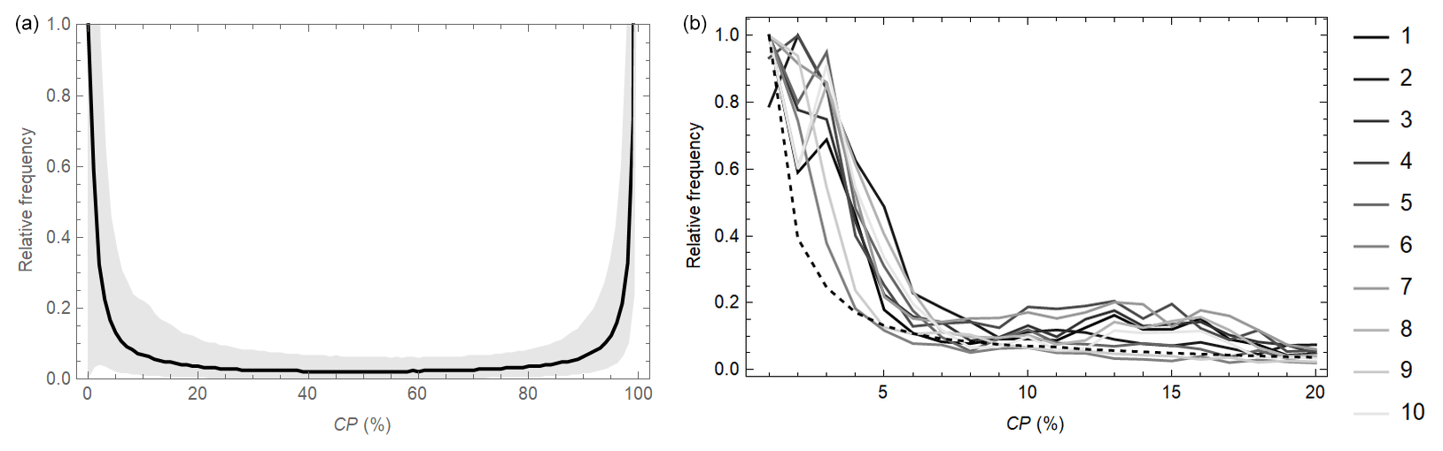
Figure 1(a) The median (solid line) and the 80 % variation range (grey shaded area) of the pixelwise cloud probability distributions for June 2012. Every fifth CP end-product pixel () available globally is included in the statistics. The frequencies are scaled with the median value at CP=0 %. (b) Ten largest pixelwise relative cloud probability distributions and the mean (dashed curve) of all CP distributions scaled with its maximum value. The solar zenith angle is restricted to not exceed 70∘.
The satellite-based CP values provided by the PPS software at GAC resolution are used in Sect. 3.1.2 as the basis for simulations of the effect of cloud fraction on the surface albedo. The CP is taken to statistically represent the cloud fraction, and only values smaller than 20 % were used in this study in order to achieve high accuracy for the surface albedo estimate. In principle, a CP value of 50 % could be suggested at first sight, but it would then mean that there is a fairly high risk that a truly cloudy pixel could be mistaken for being cloud-free. In addition, the cloud probability is linked to the optical thicknesses of clouds, meaning that optically thick clouds are easier to detect than thinner clouds (so they have higher CP values). Thus, to reduce the risk of mistaking clouds with relatively high optical thicknesses for an absence of clouds, a lower CP threshold should be used. A reasonable value that reduces this risk of misclassification but still allows a large enough sample of cloud-free cases is a CP value of 20 %. As the data mass even for every fifth pixel is quite large (620 400 individual CP values), the data were still reduced for the simulations as follows. First the ten largest distributions were taken because they are statistically representative. Then every 50th set in decreasing order of the number of points in the distribution was taken. Altogether, 612 CP distributions were used in the simulations. The reason that very small distributions (the smallest set had only 14 CP values) were also used in the simulations was that such cases also appear when deriving monthly albedo means using satellite data. For these data, the cloud probability mostly did not correlate with the solar zenith or azimuth angle. Hence, the simulations combining any CP values with any surface albedo values can be carried out without needing to pay attention to the solar angle. Later, as the SAL product is currently not normalized to any specific solar zenith angle, the results of Sect. 3.1 can be applied in SAL processing without further consideration of the effects of the solar angle on the results.
The cloud-free surface albedo estimates of CLARA-A3 will be estimated using the TOA reflectance and CP values available on a pixel basis (Fig. 2). First, the TOA reflectance values with CP>20 % are discarded, as well as values flagged as low quality by the PPS software, for example because of sun glints. Then the atmospheric correction is carried out in the same way for all remaining TOA reflectances, independently of the cloud probability. Finally, the monthly mean cloud-free surface albedo is estimated using the atmospherically corrected reflectances and corresponding CP values. The main points of the theoretical background for the cloudy surface albedo distributions (Manninen et al., 2004) are summarized in Sect. 3.1.1. The adaptation of the theoretical approach to use cloud probability data is described in Sect. 3.1.2, and finally the formulas for deriving the cloud-free monthly mean surface albedo estimates are provided in Sect. 3.2.
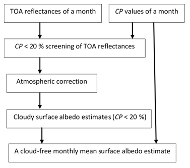
Figure 2Flow diagram of the estimation of cloud-free monthly mean surface albedo values on pixel basis starting from the TOA reflectance and CP values of the month in question.
3.1 Simulation of cloudy surface albedo distributions
3.1.1 Theoretical cloud distributions
The cloud fraction varies between the two extremes, zero and unity, with varying weather conditions. When estimating the cloud fraction distribution over the entire globe at a very coarse spatial resolution, however, it is possible that the extreme values are not achieved at all. The ultimate limit is the planetary cloudiness, which is on average about 66 % according to the latest report from the Global Energy and Water Exchanges (GEWEX) cloud assessment study (Stubenrauch et al., 2022), with the annual variation being about ±5 % (Karlsson and Devasthale, 2018). On the other hand, at very high spatial resolution, the cloud fraction is typically clearly dominated by the extreme values, as shown by ceilometer observations for example (Manninen et al., 2004). Although the cloud probability estimation is complicated by various kinds of uncertainties, the observed cloud fractions based on AVHRR data showed a U-curve-resembling distribution at both the original 1.1 km (Manninen et al., 2004) and the GAC resolution of ∼5 km. The median and 80 % variation range of the relative CP distributions are shown in Fig. 1 for every fifth CP (and SAL) end-product pixel () available globally in June 2012. The leftmost part of the U-curve is shown Fig. 1 for a few example end-product pixels. Thus, it is more common to have completely cloud-free and completely cloudy pixels, but all intermediate values are also possible. An adequate functional dependence for fitting the observed cloud fraction curves seems to be (Manninen et al., 2004)
where k is the cloud cover percentage and b and c are parameters that depend on the spatial resolution.
The elevation of the sun dominates the diurnal variation of the surface black-sky albedo (Briegleb and Ramanathan, 1982; Briegleb et al., 1986; Yang et al., 2008; Manninen et al., 2020). The diurnal albedo distribution is almost symmetric in snow-free areas when the surface albedo is normalized with respect to midday, although the albedo is typically slightly lower in the morning than in the afternoon for the same solar zenith angle due to the presence of dew (Mayor et al., 1996). For snow cover during the melting season, the albedo tends to almost linearly decrease during the day (Pirazzini, 2004; Manninen et al., 2020, 2021). In addition, the seasonal variation within 1 month may cause a slight skewness in the albedo distribution.
The albedo of the surface and clouds should dominate the albedo distribution because perfectly cloudy and perfectly clear skies are much more common than intermediate cloudiness. As long as the land-use class does not change, the snow-free surface albedo typically shows only moderate seasonal variation, but the albedo of clouds varies in a wide range with varying cloud type (Brisson et al., 1999). Therefore, the monthly albedo distribution of a snow-free surface usually constitutes only one distinct peak, which is located roughly at the surface albedo value. This is also the case for snow cover in midwinter conditions, but during the melting season the distribution is much broader (Manninen et al., 2019). However, a Gaussian monthly albedo distribution f(α) is a reasonable approximation for both snow-free and snow-covered surfaces, i.e.
where is the surface albedo average, σx is the standard deviation of the surface albedo distribution and α denotes the albedo variable. The monthly albedo distribution observed by optical satellite radiometers can be described as a combination of the surface albedo distribution, the cloud coverage distribution and the cloud shadow distribution (Manninen et al., 2004). The surface albedo distribution normalized with respect to midday is typically reasonably close to a Gaussian distribution. At high resolution (50 m) the cloud albedo has been observed to present a Weibull distribution (Koren and Joseph, 2000). At GAC resolution, a pixel may contain several layers of diverse cloud types, and the time window for the distribution is 1 month. Consequently, the albedo distribution of cloudy pixels is then a random combination of single cloud type distributions. Hence, the cloud albedo distribution at GAC resolution can be assumed to be Gaussian, although the standard deviation may be so large that the result is essentially the same as for a uniform distribution. No actual distribution shape is provided for shadows because their existence requires several conditions to apply simultaneously: (1) the pixel in question must be clear, (2) there must be a cloud close enough in the neighbourhood, (3) the sun's elevation and azimuth angles must be such that the sun is on the same line as that between the pixel in question and the cloud casting the shadow. Since slightly shadowed pixels are more probable than completely shadowed pixels, an exponentially decaying distribution was assumed for shadows:
where p is a uniform random variable in the range [0,1]. Then the probability density function (PDF) fs of the possibly shaded pixels is defined as an integral of the product of the individual PDFs of the shadow p and the surface albedo value x. The Kronecker delta function (δ) is included in the integral to restrict the integration to possible combinations of α, p and x and to only include cases with the cloud fraction k=0, so that (Manninen et al., 2004) the probability density function fs for possibly shaded cloud-free pixels is
assuming that the lowest albedo value caused by shadowing is half the true value. This assumption is based on empirical observations made using AVHRR data (Manninen et al., 2004).
The theoretical monthly albedo probability density function of cloudy pixels fc(α) is likewise defined as an integral of the product of the individual PDFs of the cloud fraction k (given here in percent), the cloud albedo value y, and the surface albedo value x. Again, the Kronecker delta function is included in the integral to restrict the integration to possible combinations of α, k, x and y so that
where is the cloud albedo average and σy is the standard deviation of the cloud albedo. The cloud albedo distribution is assumed here to be Gaussian, but sometimes the standard deviation is so large that the result is essentially the same as for a uniform distribution. The total PDF ft(α) covering all cases is
The location of the local maxima (and minima) of the albedo distributions of Eqs. (4) and (5) correspond to albedo values α for which . Since the integrals cannot be determined in closed form, no explicit relationship between the peaks of the PDF of the true surface albedo f(x) and the PDF of the total albedo ft(α) can be derived. Thus, the albedo PDFs are simulated numerically.
For cloud-free cases, the average surface albedo value of an experimental albedo distribution can be determined as the mean of the upper and lower half-height locations of the albedo distribution (Manninen et al., 2004). For the theoretical Gaussian distribution, this equals the mean value precisely. For cloudy cases, the total albedo distribution is mostly not symmetric, and using the mean of the lower and upper half-height albedo values results in the overestimation of low surface albedo mean values and the underestimation of high surface albedo mean values. It is not possible to derive a functional relationship in closed form between the clear sky and cloudy albedo means, even for theoretical distributions. In addition, the cloud fraction and type vary over wide ranges, so nothing can be assumed concerning the shape of the cloudy albedo peak. It may be distinctly skewed or almost symmetric. It may dominate the whole distribution, or the background may be at the half-height level of the peak. Therefore, robust parameters assuming nothing regarding the shape of the peak are sought for determining the mean surface albedo.
In a previous study, the half-height width and the -height width of the cloudy albedo distribution peak were shown to be suitable for true albedo value determination (Manninen et al., 2004). However, constructing distributions and determining the peak widths is numerically a very slow process. This is therefore not feasible when processing a long time series (∼40 years) globally (1440×720 pixels), even on a monthly basis. Therefore, in this study, we present a solution that can be used to estimate the surface albedo peak value without the need to construct the distribution. It is derived from simulations of cloudy albedo distributions based on observed statistics of newly available cloud probability values (see Sect. 3.1.2).
3.1.2 Satellite-based cloud distributions
The satellite-based cloud probability data provided by the PPS software (Karlsson et al., 2020) were used as proxies for cloud fractions. The total albedo distributions were calculated separately for each pixelwise CP distribution fCP(CP). Thus, the equations to use for satellite-based versions of the cloud-free, but possibly shaded, pixel distribution fs and the cloudy pixel distribution fc, denoted fSs and fSc, respectively, for each individual pixelwise cloud probability distribution are now
where k is the cloud probability discretized to integers in the range [1,19] because only CP values smaller than 20 % are allowed in order to achieve high estimation accuracy. As larger CP values than that are not used in the analysis, it is sufficient to replace the term in Eq. (5) with exp (−d k). The parameter d=0.1 is used to give even more weight to less-cloudy albedo retrievals while also allowing some weight (0.135) to be given to the 20 % cloud probability cases. The choice of the value of d is a compromise between theoretical accuracy and the desire to avoid the dominance of individual completely cloud-free retrievals. The reason that Eq. (7) is not integrated over the parameter p, as in Eq. (4), is purely practical: the data mass is too large for that. Hence, just one random shadow value is taken into account per CP. Each cloud probability distribution is combined with different values of the surface albedo distribution using random weights to improve the generalization of the results, as satellites observe samples of the surface albedo distribution in varying cloud conditions. The total albedo distribution fSt(α) is then derived as a combination of those two alternatives as before using Eq. (6), where ft, fs and fc are replaced by fSt, fSs and fSc, respectively. The first estimate of the mean surface albedo is then obtained from n individual albedo values as follows:
The monthly standard deviation, skewness and kurtosis are then calculated similarly using the total albedo distribution as weights. When a sufficient number of cloud-free pixels are present, this formula will give a good estimate for the surface albedo. However, if all pixels have 20 % probability, the above formula will approach the albedo value corresponding to 20 % cloud probability, not 0 % cloud probability. Hence, an additional correction term is applied to retrieve the final albedo estimate in the form
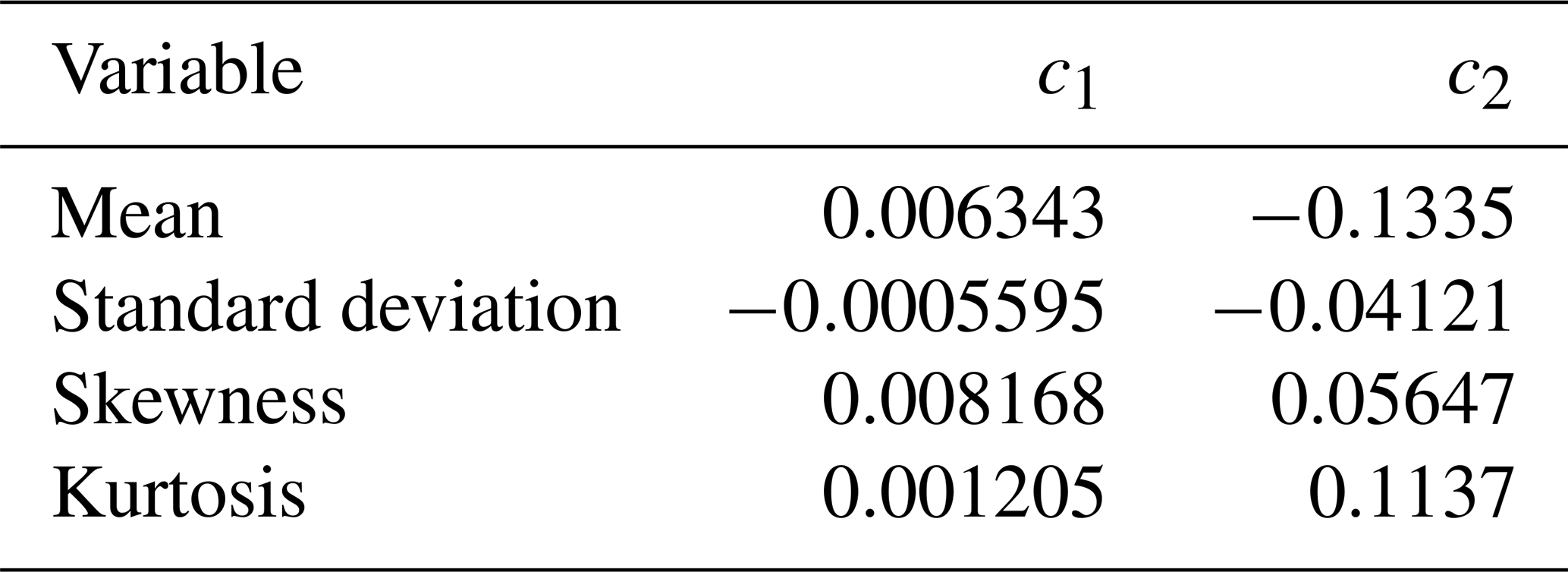
where is the monthly mean cloud probability of the CP values within the range [0 %,20 %), and the parameters c1 and c2 are determined empirically on the basis of the simulations. The assumed mean and standard deviation for the cloud albedo were 60 % and 20 %, respectively, and the calculations were made for a Gaussian surface albedo with mean values of 10 %, 20 %, 30 %, 40 %, 50 %, 60 %, 70 % and 80 % and with a standard deviation of 2 %. The values of c1 and c2 that produce the best fit of the estimated albedos to the true ones are given in Table 1. This formula adjusts the albedo estimate only when exceeds zero. The standard deviation, skewness and kurtosis estimates based on are corrected similarly using the correction factor in the brackets of Eq. (10), but with the dedicated parameter values of c1 and c2 given in Table 1.
Table 1Parameter values for Eq. (10) for the monthly mean, standard deviation, skewness and kurtosis of the surface albedo.
3.2 Surface albedo retrieval algorithm
The surface albedo algorithm used in the Climate-SAF project starts with atmospheric correction carried out using the SMAC method (Rahman and Dedieu, 1994; Proud et al., 2010). The next step is to determine the albedo values for the visible and near-infrared channels with the generally used formulas and coefficients for the bidirectional reflectance distribution functions (BRDFs) of various land use classes, which are taken from a land cover product (Roujean et al., 1992; Wu et al., 1995; Hansen et al., 2000). A topography correction is carried out in mountainous areas (Manninen et al., 2011). Finally, a broad-band conversion is carried out (Liang, 2000; Liang et al., 2002). Solar zenith angle normalization is not currently used; this is because, during product development, there was no generally applicable formula for all surface types, including melting snow (Manninen et al., 2020). The previous SAL versions (Riihelä et al., 2013; Karlsson et al., 2017; Anttila et al., 2018) required that cloud masking only applied the SAL algorithm to nominated clear-sky pixels.
For the next release, CLARA-A3 SAL, the cloud probability values (CP) provided by the PPS software (Karlsson et al., 2020) will be available, and the black-sky surface albedo (Lucht et al., 2000; Róman et al., 2010) retrieval will be based on pixels with cloud probabilities not exceeding 20 %. The albedo processing is first carried out as if all those pixels were completely cloud-free, i.e. the atmospheric correction for AOD, water vapour, air mass and ozone is made. Then the monthly mean values are approximated using a similar approach to that in Sect. 3.1.2:
The theoretically motivated form of Eq. (10) for correcting was found to result in slight black-sky albedo overestimation for large albedo values (especially for sea ice) when compared to previous albedo time series. Since Eq. (11) is not a precise theoretical formula for deriving the cloud-free albedo using possibly cloudy data, but rather a practical statistical approach for its estimation, it is understandable that a theoretical correction factor form may not be optimal either. Thus, finally, an ordinary linear-regression-based empirical correction of was derived using the albedo simulations (Sect. 3.1.2). Hence, the final monthly mean albedo estimates were derived instead of Eq. (10) using the following formula:
The difference between and is rather small and consequently the standard deviation, skewness and kurtosis were still corrected using Eq. (10).
4.1 Simulated distributions
Albedo distributions were simulated for surfaces with Gaussian mean albedo values of 10 %, 20 %, 30 %, 40 %, 50 %, 60 %, 70 % and 80 % and a standard deviation of 2 %. Examples are shown in Fig. 3. The Gaussian mean cloud albedo was taken to be 60 %, with a standard deviation of 20 %. For convenience, all distributions are scaled so that the maximum equals unity instead of using the common normalization of PDFs, which would set the integral to unity and consequently cause varying peak heights. Obviously, for relatively low surface albedo values (such as those of vegetation), the clouds cause a tail at the high end of the albedo distribution; for high albedo values (such as those of snow), a tail occurs at the low end. For albedo values close to the cloud albedo (such as sea-ice albedo values), the distribution spreads to both low and high values. The bump at the mean cloud albedo is more distinct for high b and c in Eq. (5). Due to the larger standard deviation of the cloud albedo distribution and the variation of the cloud probability, the surface albedo distribution peak still dominates the total distribution.

Figure 3Examples of simulated cloud albedo distributions for diverse values of the parameters b (blue shades) and c (shown as diverse dashed lines) in Eq. (5). The example surface albedo values are assumed to be Gaussian, with mean values of 20 % (a), 50 % (b) and 80 % (c) and a standard deviation of 2 %. The mean surface albedo is shown as a red line and the distribution as a yellow curve. The parameter p in Eq. (4) took a random value in the range [0,1]. The example cloud albedo value is assumed to be Gaussian, with a mean of 60 % and a standard deviation of 20 %.
Albedo distributions were also derived using the empirical CP pixelwise distributions and Eqs. (11) and (10). The results were compared with the true values (Table 2). For the simulated Gaussian albedo distributions, the obtained estimation accuracy is very good: the mean absolute difference is 0.48 % and the 90 % quantile for the mean value is 1.1 % (absolute albedo percentage). The relative mean albedo difference is 1.1 % and the 90 % quantile for the relative difference is 2.2 %. However, larger deviations also appear: the maximum mean albedo error is 2.8 % (absolute percentage) and the relative mean albedo error is 7.8 %. The effect of the number of individual points in the simulation on the accuracy and relative accuracy of the albedo estimation is shown in Fig. 4. Naturally, including a large number of points increases the accuracy, but the effect is not dramatic. This is important from the point of view of satellite images, because the number of individual points used to obtain a monthly mean may be quite small in areas where the sun's elevation is typically small or the sky is cloudy.
Table 2Simulated statistics for the absolute and relative differences in estimated (∧) and true values of albedo (α), standard deviation (σ) skewness (γ) and kurtosis (β). The calculations were made for albedo values of 10 %, 20 %, 30 %, 40 %, 50 %, 60 %, 70 % and 80 %. The albedo values are in the range 0 %–100 %.
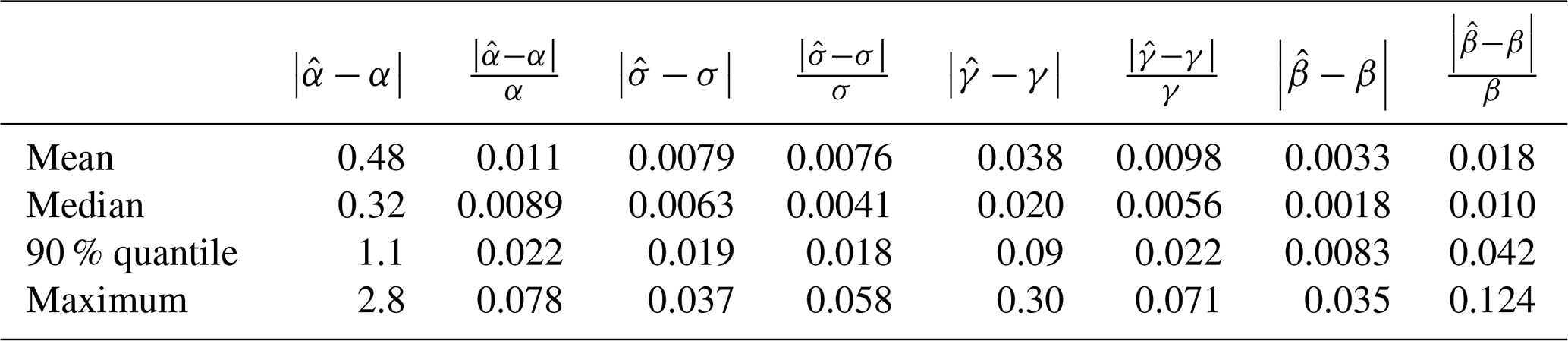
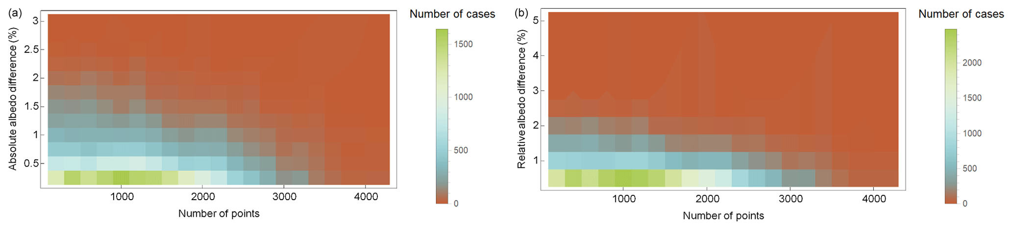
Figure 4The relationship between the number of points in the cloud distribution and the simulated mean (a) and relative mean (b) albedo accuracy.
The very high accuracy is partly due to the assumed purely Gaussian surface albedo distributions that are provided for the whole range [0 %,100 %] with an increment of 1 %. For satellite data, the surface albedo distributions are patchy, and the sampling may be biased to certain solar zenith angle values. In addition, the distributions may clearly deviate from being Gaussian. Moreover, the number of individual satellite-based albedo estimates per pixel may be much smaller than the 101 used in these simulations. Hence, such high accuracy is not expected to be achieved for satellite-based albedo estimates, but in principle this approach is capable of achieving very high albedo estimation accuracy.

Figure 5The albedo retrieval distributions at Desert Rock, Payerne and Southern Great Plains in April 2009 and Syowa in November 2008. The cloud probability values of the individual black-sky satellite-based estimates are indicated by colours. The monthly mean estimate is shown as a red line. The in situ measured monthly blue-sky albedo distribution is shown in blue.
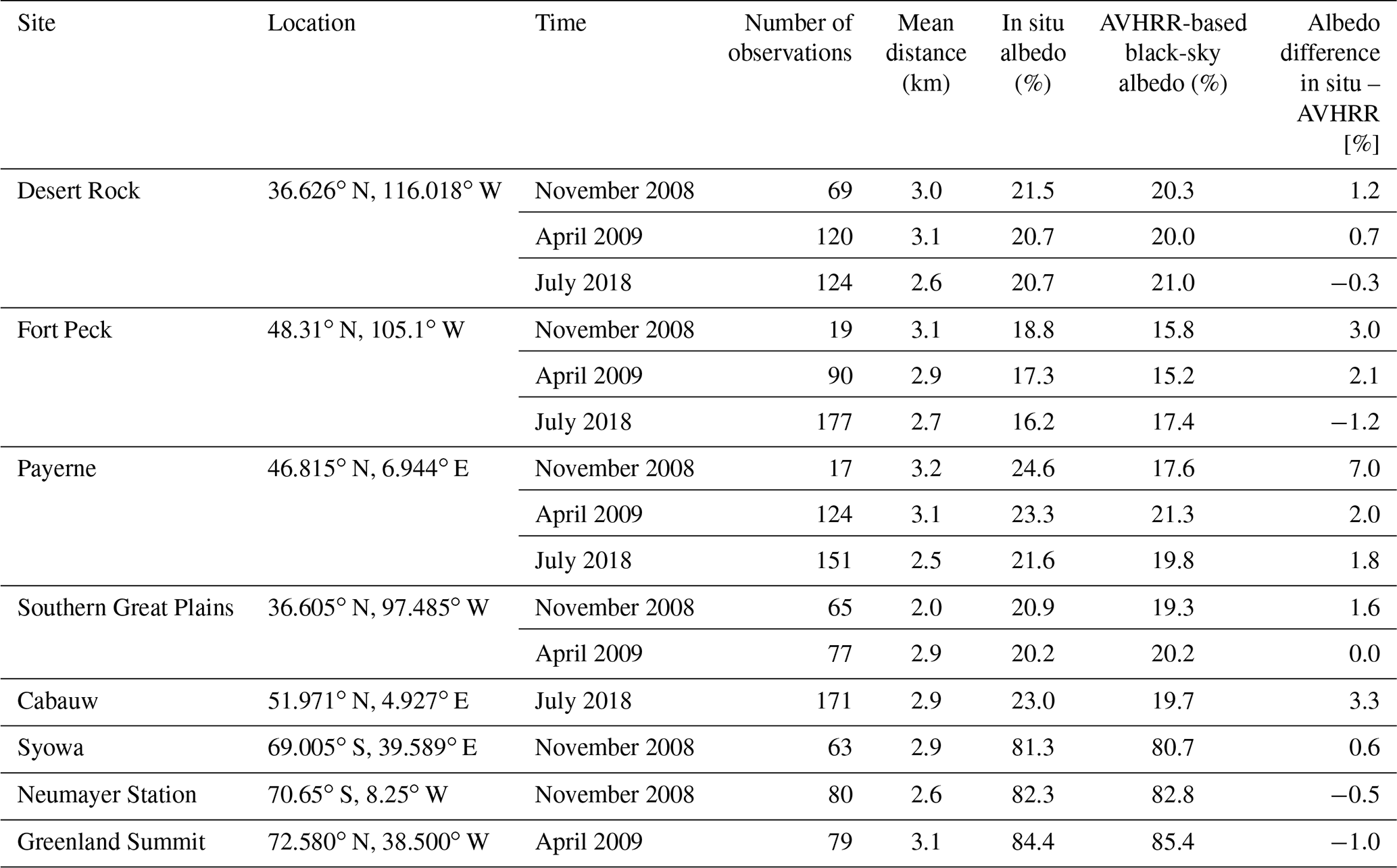
Table 3Monthly mean black-sky surface albedo values based on AVHRR reflectance and CP values and the monthly mean values of the corresponding times of in situ surface albedo measurements for several BSRN in situ sites (König-Langlo et al., 2013; Driemel et al., 2018): Desert Rock (Augustine, 2009a, b, 2019a), Fort Peck (Augustine, 2009c, d, 2019b), Payerne (Vuilleumier, 2010a, b, 2019), Southern Great Plains (Long, 2009a, b), Cabauw (Knap, 2018), Syowa (Yamanouchi, 2010) and Neumayer Station (König-Langlo, 2009). Data from the Greenland Summit in situ site is also included (Steffen et al., 1996). The number of observations included in the mean value are given, as well as the mean distance of the satellite pixels from the in situ measurement mast.
4.2 Satellite-based distributions
Histograms of surface albedos at GAC resolution for 1 month were constructed using the new CLARA-A3 SAL algorithm for the chosen relatively homogeneous test sites of Desert Rock (36.626∘ N, 116.018∘ W), Payerne (46.815∘ N, 6.944∘ E), Southern Great Plains (36.605∘ N, 97.485∘ W) and Greenland Summit (72.580∘ N, 38.500∘ W), applying a 1 % bin width. These are presented in Fig. 5. The corresponding in situ albedo distributions are shown as well. Only points for which both a satellite overpass and an in situ measurement were available within a 15 min time window are shown. Monthly means derived from simultaneous in situ and satellite-based albedo values are given for several sites in Table 3. Since the in situ irradiance measurements also contain a contribution from the atmosphere, the comparison to a black-sky surface albedo estimate contains some inherent discrepancy, but for dark surfaces the in situ albedo values should be only slightly larger than the satellite-based values. The difference increases with increasing AOD due to the resulting increase in atmospheric scattering, which plays a greater role as the surface scattering decreases. For bright targets, such as snow, the effect of the atmosphere reduces the measured surface albedo value because the target is such a strong scatterer that the increase in atmospheric scattering due to the AOD is smaller than the reduction in target scattering due to the smaller irradiance at the surface. In addition, the satellite pixel diameter is about 25 km, and in situ measurements typically characterize footprints of some hundreds of square metres. Possible land-cover inhomogeneity around the measurement site inevitably causes a discrepancy between the satellite and in situ values (Riihelä et al., 2013). The difference between in situ and satellite-based values is typically largest in winter conditions (November), as occasional snowfalls may increase the in situ albedo markedly whereas the satellite still detects large snow-free dark targets (such as Lac Neuchâtel in Payerne), and scenery containing coniferous forests (e.g. in Fort Peck) are mostly relatively dark, even in snow-covered conditions. The reason for the high in situ albedo of Cabauw as compared to the satellite-based albedo is the typically thick atmosphere of Cabauw. The difference between the mean albedo values slight increases as the number of individual values used to find the means decreases and with increasing distance between the mean of the satellite pixel locations and the measurement point.
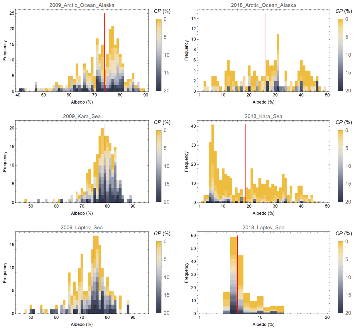
Figure 6The albedo retrieval distributions at the Arctic Ocean (73.370∘ N, 139.180∘ W), Kara Sea (2.680∘ N, 62.860∘ E) and Laptev Sea (75.320∘ N, 125.720∘ E) in April 2009 and July 2018. The cloud probability values of the individual black-sky satellite-based estimates are indicated by colours. The monthly mean estimate is shown as a red line.
In sea-ice areas, the variation in the surface albedo within 1 month may be large due to large amounts of open water and movements of the ice field. Examples of this are shown in Fig. 6 for sites in the Arctic Ocean off Alaska, the Kara Sea and the Laptev Sea. In June 2009 there was still quite a lot of sea ice in all three areas, whereas in June 2018, due to climate change, all of those sites were relatively ice free – especially the Laptev Sea, which had a large area of open water (EUMETSAT Ocean and Sea Ice Satellite Application Facility, 2021). When the sea-ice concentration varies markedly, the monthly mean albedo estimate is greatly affected by the timing of days with a small probability of cloud.
This study demonstrates the use of cloud probability information for surface albedo retrieval. At the time of the study, only 1 month of cloud probability data was available globally. In June, the Northern Hemisphere is covered best, but high Southern Hemisphere latitudes (mainly Antarctica) are missing because of the low solar zenith angle values. As the cloud cover varies seasonally, it would be desirable to update the parameter values of this study (Table 1 and the form of Eq. 12) using global cloud probability data for 1 year. However, despite the rather limited cloud probability statistics of this study, the achieved estimation accuracy of monthly albedo means was satisfactory, and the values were in line with the in situ measurements.
Typically, the surface albedo of a snow-free surface depends on the solar zenith angle such that the minimum is obtained at midday and the albedo is azimuthally symmetric (Briegleb and Ramanathan, 1982; Briegleb et al., 1986; Yang et al., 2008; Manninen et al., 2020). Also, for snow outside the melting season, the dependence is similar unless the surroundings are very anisotropic. If the whole diurnal albedo distribution from satellite data were to become available, it might be a good idea to take that into account in the simulations and when deriving the parameter values used for albedo estimation (Table 1). However, a satellite-based AVHRR instrument observes a site typically only once per day and at about the same time on successive days. Hence, the use of a Gaussian albedo distribution as the basis for the simulations seemed reasonable.
To provide a comparison with the approach used in this study, the surface albedo was also estimated using a standard cloud-masking procedure. Then the monthly mean albedo was directly obtained as the average value of the cloud-free masked pixels, but we again restricted the processing to cases with CP<20 %. The results are shown in Fig. 7. Obviously, using the cloud mask, one typically gets slightly higher albedo values for snow-free areas than when using the cloud probability values, and lower albedo values for snow-covered areas (Greenland Summit, Syowa and Neumayer). This is exactly how cloudiness would affect the albedo retrieval (Sect. 3.1.1), and it supports the notion that the CP-based approach of this study can exclude the effect of cloud contamination of the TOA reflectance values more effectively than plain cloud mask usage. In addition, the difference between the estimates given by the two methods is typically largest for snow-covered areas, where cloud discrimination is very challenging, especially when the sun's elevation is low (Karlsson and Håkansson, 2018).
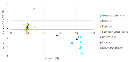
Figure 7The difference between the monthly mean surface albedo estimates derived using the cloud masking (CM) and cloud probability (CP) approaches for several Northern Hemisphere test sites in July 1979, April 1981, November 2008, April 2009, July 2018 and April 2020. For Greenland Summit, no satellite albedo data were available for November 2008 due to low solar elevation. For the Southern Hemisphere sites Syowa and Neumayer Station, data were available for January 1979 and November 2008.
In Cabauw, the largest difference between the two approaches occurred in November 2008, when there were only three points available that matched the in situ measurement times due to the low solar elevation, and the satellite-based albedo estimate varied in the range 20.6 %–43.3 %. The largest value was masked cloud free, but the CP value was 19.8 % and the high reflectivity may also have been due to patchy snow or partial cloud contamination. Snow might also explain the fraction of cloud masked pixels with very small CP values.
The CLARA-A3 SAL will be derived using the CP values instead of the binary cloud mask. The pentad means will be derived in a technically similar way to the monthly means using pentad distributions of CP. Future studies of the CLARA-A3 CP and cloud mask characteristics will show whether it would be desirable to use both the cloud mask and the CP values as the basis for SAL estimation. In addition, the parameter values used in Eqs. (10) and (12) would benefit from an updated analysis using CP data for a whole year as input.
Since the surface albedo is directly related to the TOA reflectance value, the approach presented here for surface albedo estimation could also be adapted to estimate other reflectance-associated surface parameters instead of using traditional cloud masking when a time window containing several images is of interest. Naturally, in general, the reliability of the method increases with the number of points to be averaged.
Cloud probability values provided by the CM SAF CLARA-A3 data record will offer a good alternative to binary cloud masking for surface reflectance and albedo estimation when the goal is not to study individual images but statistics within a time window. Simple weighted averaging on the basis of the cloud probability values and a basic linear regression correction for biased no clear-sky events containing time windows provide good estimates for surface albedo.
| Symbol | Meaning |
| c1 | Empirical coefficient used in final albedo |
| estimate retrieval | |
| c2 | Empirical coefficient used in final albedo |
| estimate retrieval | |
| CP | Cloud probability |
| Monthly mean cloud probability | |
| d | Weight parameter for albedo monthly |
| mean retrieval | |
| f(α) | Albedo distribution |
| fc(α) | Probability density function of albedo for |
| cloudy pixels | |
| fCP(CP) | Pixelwise cloud probability density function |
| fk(k) | Cloud distribution based on cloud fraction |
| fp(p) | Probability density function of shadows |
| fs(α) | Probability density function of albedo for |
| possibly shaded pixels | |
| fSc(α) | Satellite-based probability density function of |
| albedo for cloudy pixels | |
| fSs(α) | Satellite-based probability density function of |
| albedo for possibly shaded pixels | |
| fSt(α) | Satellite-based total probability density |
| function of albedo | |
| ft(α) | Total probability density function of albedo |
| k | Cloud fraction |
| p | Probability of shadow |
| α | Albedo |
| Monthly mean albedo, first estimate | |
| Monthly mean albedo, final estimate | |
| β | Kurtosis |
| γ | Skewness |
| σ | Standard deviation |
No special code to deliver, only very basic calculations carried out using Mathematica.
The data used in this study were temporary development data and will not be archived or get a DOI number.
TM, EJ and NS carried out the theoretical development. TM performed the simulations and albedo quality analysis. AR provided in situ data and participated in the albedo quality analysis. KGK developed and provided the cloud probability data and related information used in the study. Everybody participated in writing the paper.
The contact author has declared that neither they nor their co-authors have any competing interests.
Publisher’s note: Copernicus Publications remains neutral with regard to jurisdictional claims in published maps and institutional affiliations.
This study was carried out within the Satellite Application Facility on Climate Monitoring (CM SAF) project, financially supported by EUMETSAT. The authors wish to acknowledge the valuable support from the World Radiation Monitoring Center (WRMC) in granting permission to use the BSRN data in this study. The Greenland Climate Network is acknowledged for the provision of data from Summit Station, Greenland. They also wish to thank other colleagues from FMI and the Climate-SAF project for co-operation during various parts of the work.
This research has been supported by the European Organization for the Exploitation of Meteorological Satellites (Satellite Application Facility on Climate Monitoring, CM SAF).
This paper was edited by Andrew Sayer and reviewed by two anonymous referees.
Anttila, K., Manninen, T., Jääskeläinen, E., Riihelä, A., and Lahtinen, P.: The Role of Climate and Land Use in the Changes in Surface Albedo Prior to Snow Melt and the Timing of Melt Season of Seasonal Snow in Northern Land Areas of 40∘ N–80∘ N during 1982–2015, Remote Sens., 10, 1619, https://doi.org/10.3390/rs10101619, 2018.
Augustine, J.: Basic measurements of radiation at station Desert Rock (2008-11), NOAA – Air Resources Laboratory, Boulder, PANGAEA [data set], https://doi.org/10.1594/PANGAEA.719888, 2009a.
Augustine, J.: Basic measurements of radiation at station Desert Rock (2009-04), NOAA – Air Resources Laboratory, Boulder, PANGAEA [data set], https://doi.org/10.1594/PANGAEA.719908, 2009b.
Augustine, J.: Basic measurements of radiation at station Fort Peck (2008-11), NOAA – Air Resources Laboratory, Boulder, PANGAEA [data set], https://doi.org/10.1594/PANGAEA.721298, 2009c.
Augustine, J.: Basic measurements of radiation at station Fort Peck (2009-04), NOAA – Air Resources Laboratory, Boulder, PANGAEA [data set], https://doi.org/10.1594/PANGAEA.721314, 2009d.
Augustine, J.: Basic measurements of radiation at station Desert Rock (2018-07), NOAA – Air Resources Laboratory, Boulder, PANGAEA [data set], https://doi.org/10.1594/PANGAEA.899138, 2019a.
Augustine, J.: Basic measurements of radiation at station Fort Peck (2018-07), NOAA – Air Resources Laboratory, Boulder, PANGAEA [data set], https://doi.org/10.1594/PANGAEA.900179, 2019b.
Briegleb, B. and Ramanathan, V.: Spectral and diurnal variations in clear sky planetary albedo, J. Appl. Meteorol., 21, 1160–1171, 1982.
Briegleb, B., Minnis, P., Ramanathan, V., and Harrison, E.: Comparison of regional clear-sky albedos inferred from satellite observations and model computations, J. Clim. Appl. Meteorol., 25, 214–226, 1986.
Brisson, A., Le Borgne, P., and Marsouin, A.: Development of algorithms for Surface Solar Irradiance retrieval at O&SI SAF Low and Mid Latitudes, Ocean & Sea Ice SAF Scientific Report, 31 pp., 1999.
Devasthale, A., Raspaud, M., Schlundt, C., Hanschmann, T., Finkensieper, S., Dybbroe, A., Hörnquist, S., Håkansson, N., Stengel, M., and Karlsson, K.-G.: PyGAC: An open-source, community-driven Python interface to preprocess the nearly 40-year AVHRR Global Area Coverage (GAC) data record, GSICS Quarterly, Summer Issue 2017, 11, 3–5, https://doi.org/10.7289/V5R78CFR, 2017.
Driemel, A., Augustine, J., Behrens, K., Colle, S., Cox, C., Cuevas-Agulló, E., Denn, F. M., Duprat, T., Fukuda, M., Grobe, H., Haeffelin, M., Hodges, G., Hyett, N., Ijima, O., Kallis, A., Knap, W., Kustov, V., Long, C. N., Longenecker, D., Lupi, A., Maturilli, M., Mimouni, M., Ntsangwane, L., Ogihara, H., Olano, X., Olefs, M., Omori, M., Passamani, L., Pereira, E. B., Schmithüsen, H., Schumacher, S., Sieger, R., Tamlyn, J., Vogt, R., Vuilleumier, L., Xia, X., Ohmura, A., and König-Langlo, G.: Baseline Surface Radiation Network (BSRN): structure and data description (1992–2017), Earth Syst. Sci. Data, 10, 1491–1501, https://doi.org/10.5194/essd-10-1491-2018, 2018.
Dybbroe, A., Thoss, A., and Karlsson, K.-G.: NWCSAF AVHRR cloud detection and analysis using dynamic thresholds and radiative transfer modelling – Part I: Algorithm description, J. Appl. Meteorol., 44, 39–54, 2005.
EUMETSAT Ocean and Sea Ice Satellite Application Facility: Global sea ice concentration interim climate data record 2016-onwards (v2.0, 2017), OSI-430-b, OSI SAF FTP server/EUMETSAT Data Center [data set], https://doi.org/10.15770/EUM_SAF_OSI_NRT_2008, 2021.
GCOS: The Global Observing System for Climate: Implementation Needs, Reference Number GCOS-200, WMO, 2016.
Hansen, M. C., Defries, R. S., Townshend, J. R. G., and Sohlberg, R.: Global land cover classification at 1km spatial resolution using a classification tree approach, Int. J. Remote Sens., 21, 1331–1364, 2000.
Heidinger, A. K., Anne, V. R., and Dean, C.: Using MODIS to Estimate Cloud Contamination of the AVHRR Data Record, J. Atmos. Ocean. Tech., 19, 586–601, 2002.
Heidinger, A. K., Straka, W. C., Molling, C. C., Sullivan, J. T., and Wu, X. Q.: Deriving an inter-sensor consistent calibration for the AVHRR solar reflectance data record, Int. J. Remote Sens., 31, 6493–6517, https://doi.org/10.1080/01431161.2010.496472, 2010.
Hersbach, H., Bell, B., Berrisford, P., et al.: The ERA5 global reanalysis, Q. J. Roy. Meteor. Soc., 146, 1999–2049, https://doi.org/10.1002/qj.3803, 2020.
Jääskeläinen, E., Manninen, T., Tamminen, J., and Laine, M.: The Aerosol Index and Land Cover Class Based Atmospheric Correction Aerosol Optical Depth Time Series 1982–2014 for the SMAC Algorithm, Remote Sens., 9, 1095, https://doi.org/10.3390/rs9111095, 2017.
Karlsson, K.-G. and Devasthale, A.: Inter-Comparison and Evaluation of the Four Longest Satellite-Derived Cloud Climate Data Records: CLARA-A2, ESA Cloud CCI V3, ISCCP-HGM, and PATMOS-x, Remote Sens., 10, 1567, https://doi.org/10.3390/rs10101567, 2018.
Karlsson, K.-G. and Håkansson, N.: Characterization of AVHRR global cloud detection sensitivity based on CALIPSO-CALIOP cloud optical thickness information: demonstration of results based on the CM SAF CLARA-A2 climate data record, Atmos. Meas. Tech., 11, 633–649, https://doi.org/10.5194/amt-11-633-2018, 2018.
Karlsson, K.-G.; Johansson, E.; and Devasthale, A.: Advancing the uncertainty characterisation of cloud masking in passive satellite imagery : Probabilistic formulations for NOAA AVHRR data, Remote Sens. Environ., 158, 126–139, https://doi.org/10.1016/j.rse.2014.10.028, 2015.
Karlsson, K.-G., Anttila, K., Trentmann, J., Stengel, M., Fokke Meirink, J., Devasthale, A., Hanschmann, T., Kothe, S., Jääskeläinen, E., Sedlar, J., Benas, N., van Zadelhoff, G.-J., Schlundt, C., Stein, D., Finkensieper, S., Håkansson, N., and Hollmann, R.: CLARA-A2: the second edition of the CM SAF cloud and radiation data record from 34 years of global AVHRR data, Atmos. Chem. Phys., 17, 5809–5828, https://doi.org/10.5194/acp-17-5809-2017, 2017.
Karlsson, K.-G., Johansson, E., Håkansson, N., Sedlar, J., and Eliasson, S.: Probabilistic Cloud Masking for the Generation of CM SAF Cloud Climate Data Records from AVHRR and SEVIRI Sensors, Remote Sens., 12, 713, https://doi.org/10.3390/rs12040713, 2020.
Knap, W.: Basic and other measurements of radiation at station Cabauw (2018-07), Koninklijk Nederlands Meteorologisch Instituut, De Bilt, PANGAEA [data set], https://doi.org/10.1594/PANGAEA.892887, 2018.
König-Langlo, G.: Basic and other measurements of radiation at Neumayer Station (2008-11), Alfred Wegener Institute, Helmholtz Centre for Polar and Marine Research, Bremerhaven, PANGAEA [data set], https://doi.org/10.1594/PANGAEA.716641, 2009.
König-Langlo, G., Sieger, R., Schmithüsen, H., Bücker, A., Richter, F., and Dutton, E. G.: The Baseline Surface Radiation Network and its World Radiation Monitoring Centre at the Alfred Wegener Institute, GCOS-174, WCRP Rep. 24/2013, 30 pp., https://bsrn.awi.de/fileadmin/user_upload/bsrn.awi.de/Publications/gcos-174.pdf (last access: 12 January 2022), 2013.
Koren, I. and Joseph, J. H.: The histogram of the brightness distribution of clouds in high-resolution remotely sensed images, J. Geophys. Res., 105, 29369–29377, https://doi.org/10.1029/2000JD900394, 2000.
Liang, S.: Narrowband to broadband conversions of land surface albedo: I Algorithms, Remote Sens. Environ., 76, 213–238, 2000.
Liang, S., Shuey, C. J., Russ, A. L., Fang, H., Chen, M., Walthall, C. L., Daughtry, C. S. T., and Hunt Jr., R.: Narrowband to broadband conversions of land surface albedo: II Validation, Remote Sens. Environ., 84, 25–41, 2002.
Long, C.: Basic measurements of radiation at station Southern Great Plains (2008-11), Argonne National Laboratory, PANGAEA [data set], https://doi.org/10.1594/PANGAEA.724290, 2009a.
Long, C.: Basic measurements of radiation at station Southern Great Plains (2009-04), Argonne National Laboratory, PANGAEA [data set], https://doi.org/10.1594/PANGAEA.724300, 2009b.
Lucht, W., Schaaf, C. B., and Strahler, A. H.: An algorithm for the retrieval of Albedo from space using semiempirical BRDF models, IEEE T. Geosci. Remote, 38, 977–998, https://doi.org/10.1109/36.841980, 2000.
Manninen, T., Siljamo, N., Poutiainen, J., Vuilleumier, L., Bosveld, F., and Gratzki, A.: Cloud statistics based estimation of land surface albedo from AVHRR data, Proc. of SPIE, Remote Sensing of Clouds and the Atmosphere IX, Gran Canaria, Spain, 13–15 September 2004, SPIE, 5571, 412–423, 2004.
Manninen, T., Andersson, K., and Riihelä, A.: Topography correction of the CM-SAF surface albedo product SAL, in: Proc. 2011 EUMETSAT Meteorological Satellite Conference, Oslo, 5–9 September 2011, CD, 8 pp., 2011.
Manninen, T., Jääskeläinen, E., and Riihelä, A.: Black and White-Sky Albedo Values of Snow: In Situ Relationships for AVHRR-Based Estimation Using CLARA-A2 SAL, Can. J. Remote Sens., 45, 18 pp., https://doi.org/10.1080/07038992.2019.1632177, 2019.
Manninen, T., Jääskeläinen, E., and Riihelä, A.: Diurnal Black-Sky Surface Albedo Parameterization of Snow, J. Appl. Meteorol. Clim., 59, 1415–1428, https://doi.org/10.1175/JAMC-D-20-0036.1, 2020.
Manninen, T., Anttila, K., Jääskeläinen, E., Riihelä, A., Peltoniemi, J., Räisänen, P., Lahtinen, P., Siljamo, N., Thölix, L., Meinander, O., Kontu, A., Suokanerva, H., Pirazzini, R., Suomalainen, J., Hakala, T., Kaasalainen, S., Kaartinen, H., Kukko, A., Hautecoeur, O., and Roujean, J.-L.: Effect of small-scale snow surface roughness on snow albedo and reflectance, The Cryosphere, 15, 793–820, https://doi.org/10.5194/tc-15-793-2021, 2021.
Mayor, S., Smith Jr., W. L., Nguyen, L., Alberta, A., Minnis, P., Whitlock, C. H., and Schuster, G. L.: Asymmetry in the Diurnal Variation of Surface Albedo, Proc. of International Geoscience and Remote Sensing Symposium, IGARSS'96, Lincoln, 27–31 May 1996, 4, 1911–1913, 1996.
Pirazzini, R.: Surface albedo measurements over Antarctic sites in summer, J. Geophys. Res., 109, D20118, https://doi.org/10.1029/2004JD004617, 2004.
Proud, S. R., Rasmussen, M. O., Fensholt, R., Sandholt, I., Shisanya, C., Mutero, W., Mbow, C., and Anyamba, A.: Improving the SMAC atmospheric correction code by analysis of Meteosat Second Generation NDVI and surface reflectance data, Remote Sens. Environ., 114, 1687–1698, https://doi.org/10.1016/j.rse.2010.02.020, 2010.
Rahman, H. and Dedieu, G.: SMAC: a simplified method for the atmospheric correction of satellite measurements in the solar spectrum, Int. J. Remote Sens., 15, 123–143, https://doi.org/10.3390/rs9111095, 1994.
Riihelä, A., Manninen, T., Laine, V., Andersson, K., and Kaspar, F.: CLARA-SAL: a global 28 yr timeseries of Earth's black-sky surface albedo, Atmos. Chem. Phys., 13, 3743–3762, https://doi.org/10.5194/acp-13-3743-2013, 2013.
Román, M. O., Schaaf, C. B., Lewis, P., Gao, F., Anderson, G. P., Privette, J. L. Strahler, A. H., Woodcock, C. E., and Barnsley, M.: Assessing the coupling between surface albedo derived from MODIS and the fraction of diffuse skylight over spatially-characterized landscapes, Remote Sens. Environ., 114, 738–760, https://doi.org/10.1016/j.rse.2009.11.014, 2010.
Roujean, J.-L., Leroy, M., and Deschamps, P.-Y.: A Bidirectional Reflectance Model of the Earth's Surface for the Correction of Remote Sensing Data, J. Geophys. Res., 97, 20455–20468, 1992.
Schulz, J., Albert, P., Behr, H.-D., Caprion, D., Deneke, H., Dewitte, S., Dürr, B., Fuchs, P., Gratzki, A., Hechler, P., Hollmann, R., Johnston, S., Karlsson, K.-G., Manninen, T., Müller, R., Reuter, M., Riihelä, A., Roebeling, R., Selbach, N., Tetzlaff, A., Thomas, W., Werscheck, M., Wolters, E., and Zelenka, A.: Operational climate monitoring from space: the EUMETSAT Satellite Application Facility on Climate Monitoring (CM-SAF), Atmos. Chem. Phys., 9, 1687–1709, https://doi.org/10.5194/acp-9-1687-2009, 2009.
Steffen, K., Box, J. E., and Abdalati, W.: Greenland Climate Network: GC-Net, edited by: Colbeck, S. C., CRREL 96-27 Special Report on Glaciers, Ice Sheets and Volcanoes, trib. to M. Meier, 98–103, 1996.
Stubenrauch, C. J., Kinne, S., Heidinger, A., et al.: Lessons learned from the updated GEWEX Cloud Assessment database. In preparation, 2022.
Vuilleumier, L.: Basic and other measurements of radiation at station Payerne (2008-11), Swiss Meteorological Agency, Payerne, PANGAEA [data set], https://doi.org/10.1594/PANGAEA.735084, 2010a.
Vuilleumier, L.: Basic and other measurements of radiation at station Payerne (2009-04), Swiss Meteorological Agency, Payerne, PANGAEA [data set], https://doi.org/10.1594/PANGAEA.735299, 2010b.
Vuilleumier, L.: Basic and other measurements of radiation at station Payerne (2018-07), Swiss Meteorological Agency, Payerne, PANGAEA [data set], doi10.1594/PANGAEA.898990, 2019.
Wu, A., Li, Z., and Cihlar, J.: Effects of land cover type and greenness on advanced very high resolution radiometer bidirectional reflectances: Analysis and removal, J. Geophys. Res., 100, 9179–9192, 1995.
Yamanouchi, T.: Basic and other measurements of radiation at station Syowa (2008-11), National Institute of Polar Research, Tokyo, PANGAEA [data set], https://doi.org/10.1594/PANGAEA.741002, 2010.
Yang, F., Mitchell, K., Hou, Y.-T., Dai, Y., Zeng, X., Wang, Z., and Liang, X.-Z.: Dependence of land surface albedo on solar zenith angle: Observations and model parameterization, J. Appl. Meteorol. Climatol., 47, 2963–2982, https://doi.org/10.1175/2008JAMC1843.1, 2008.