the Creative Commons Attribution 4.0 License.
the Creative Commons Attribution 4.0 License.
 | 13 Jan 2023
Spectral replacement using machine learning methods for continuous mapping of the Geostationary Environment Monitoring Spectrometer (GEMS)
Yeeun Lee
Mina Kang
Mijin Eo
Earth radiances in the form of hyperspectral measurements contain useful information on atmospheric constituents and aerosol properties. The Geostationary Environment Monitoring Spectrometer (GEMS) is an environmental sensor measuring such hyperspectral data in the ultraviolet and visible spectral range over the Asia–Pacific region. After completion of the in-orbit test of GEMS in October 2020, bad pixels are found as one of remaining calibration issues resulting in obvious spatial gaps in the measured radiances as well as retrieved properties. To solve the fundamental cause of the issue, this study takes an approach reproducing the defective spectra with machine learning models using artificial neural network (ANN) and multivariate linear regression (Linear). Here the models are trained with defect-free measurements of GEMS after dimensionality reduction with principal component analysis (PCA). Results show that the PCA-Linear model has small reproduction errors for a narrower spectral gap and is less vulnerable to outliers with an error of 0.5 %–5 %. On the other hand, the PCA-ANN model shows better results emulating strong non-linear relations with an error of about 5 % except for the shorter wavelengths around 300 nm. It is demonstrated that dominant spectral patterns can be successfully reproduced with the models within the level of radiometric calibration accuracy of GEMS, but a limitation remains when it comes to finer spectral features. When applying the reproduced spectra to retrieval processes of cloud and ozone, cloud centroid pressure shows an error of around 1 %, while total ozone column density shows relatively higher variance. As an initial step reproducing spectral patterns for bad pixels, the current study provides the potential and limitations of machine learning methods to improve hyperspectral measurements from the geostationary orbit.
- Article
(26910 KB) - Full-text XML
- BibTeX
- EndNote


Earth radiances provide useful information on the atmospheric chemical composition, especially when it is measured in the form of many contiguous spectral bands. This type of measurement is referred to as “hyperspectral” (Bovensmann et al., 1999; Goetz et al., 1985), which is sampled with high spectral resolution to accurately describe absorption lines of targeted gaseous or particulate components (Boersma et al., 2004; Loyola et al., 2011; Hedelt et al., 2019; Manolakis et al., 2019; Kang et al., 2020). The Geostationary Environment Monitoring Spectrometer (GEMS) on-board the Geostationary Korea Multi-Purpose Satellite-2B (GEO-KOMPSAT-2B) is an environmental sensor providing such a hyperspectral measurement in the ultraviolet and visible (UV–VIS) spectral region from 300 to 500 nm with a spectral resolution of finer than 0.6 nm (Kim et al., 2020; Kang et al., 2022). Following the launch of the satellite in February 2020, the in-orbit test (IOT) of GEMS was successfully completed in October 2020 with some issues to be continuously monitored on the radiance level (Level 1B) with collected long-term measurements (Schenkeveld et al., 2017; Pan et al., 2019; Lee et al., 2020; Ludewig et al., 2020)
One of the issues to be periodically monitored is bad pixels, which refers to anomalous pixels having hot, cold, noisy or drifted readout values in raw data (Han et al., 2002; López-Alonso and Alda, 2002). The definition of bad pixels is not universal, and in this paper, it refers to all kinds of pixels having abnormal observation features. The impact of bad pixels on the GEMS data products is obvious because the given areas affected by bad pixels cannot provide any measured information. It causes spatial discontinuity in Level 1B data and retrieved properties (Level 2) by affecting retrieval processes with contaminated spectral features. The defective region is not large so far, but the area could be enlarged as time goes by (Kieffer, 1996) and the missing areas may increase, possibly including scientifically important regions, especially for environmental monitoring.
Because there is a constant measurement gap for certain areas in the GEMS field of regard (FOR), one might need alternative information for the areas for practical or scientific reasons. To supplement the information and investigate the applicability of machine learning, this study focuses on replacing the Level 1B radiances using spectral relations with simple machine learning methods. One of advantages of replacing Level 1B data (not Level 2) is that improving spectral features can be an efficient way to solve the bad-pixel issue for all Level 2 products. The proposed approach places more emphasis on efficiency and further applicability of machine learning, even though the spatial gaps in Level 2 data can be filled with a more suitable method for each product with higher accuracy (e.g., variogram or mathematical filters) (Fang et al., 2008; Katzfuss and Cressie, 2011; Guo et al., 2015; Llamas et al., 2020; Yang et al., 2021). Another advantage is that the approach helps the current retrieval algorithms to avoid bad-pixel effects without further development. The GEMS cloud height retrieval algorithm, for instance, had to modify the fitting window during the IOT because the targeted O2–O2 absorption lines (around 477 nm) are affected by bad pixels. The proposed approach, however, has the potential to reproduce the O2–O2 absorption features with the information from unaffected wavelengths (e.g., rotational Raman scattering lines). If it is successful, retrievals can avoid bad-pixel effects without further algorithm development. The main question to be answered for that is whether non-linear spectral relations could be effectively emulated with spectral replacement using machine learning techniques.
For atmospheric remote sensing, the majority of research has employed machine learning as a proxy for the radiative transfer model to retrieve geophysical states from measured spectral radiances (Loyola et al., 2018; Zhu et al., 2018; Hedelt et al., 2019). There are fewer approaches applied to obtain radiation flux (Zarzalejo et al., 2005) and even much fewer to obtain hyperspectral radiances to accurately quantify radiative forcing in climate system (Taylor et al., 2016), increase spectral resolution (Le et al., 2020) and fill in a spectral gap for inter-calibration (Wu et al., 2018). A monochromatic radiance itself rarely contains any important meaning and thus has seldom been a final target. In this study, however, radiance at each wavelength for a targeted spectral region is an important output to be reproduced with machine learning models, artificial neural network (ANN) and multivariate linear regression. Theoretically, ANN can accurately emulate non-linear relations with a simple model structure using large training data (Cybenko, 1989; Hornik et al., 1989). Machine learning methods also have a high chance to successfully process hyperspectral data because the abundant datasets make the training process more efficient after breaking the curse of dimensionality with a proper pre-processing step (Gewali et al., 2018). Principal component analysis (PCA) is applied for that in this study, which is useful to extract important information from hyperspectral measurements (Horler and Ahern, 1986; Bajorski, 2011; Li et al., 2013, 2015; Joiner et al., 2016).
The following sections are organized as follows. Section 2 introduces sensor specification of GEMS and a general description of machine learning models with model structure and hyperparameter setting. Section 3 contains model optimization results and error analysis for wide defect regions. With the optimized model, the spatial and spectral inspection is performed for reproduced radiances and retrieved properties. In Sect. 4, conclusions are presented with limitations as well as further application in future study.
2.1 Data description
2.1.1 GEMS
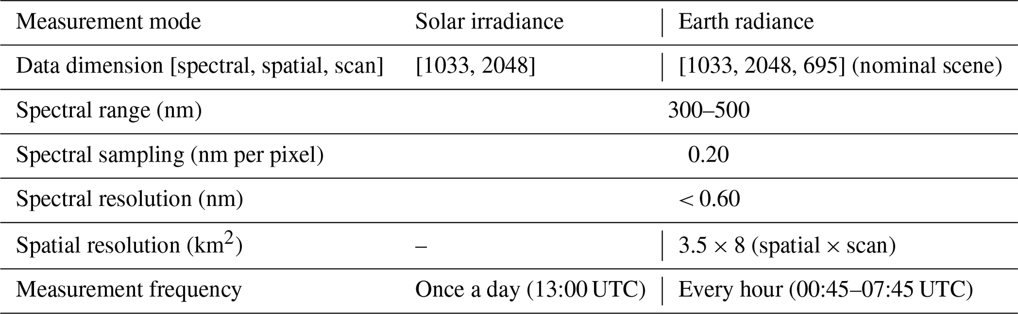
GEMS is a UV–VIS imaging spectrometer in the geostationary orbit observing the Asia–Pacific region (5∘ S–45∘ N, 75–145∘ E) with high spatial and spectral resolution to retrieve key atmospheric constituents such as ozone (O3), sulfur dioxide (SO2), nitrogen dioxide (NO2), formaldehyde (HCHO), glyoxal (CHOCHO) and aerosol properties (Kim et al., 2020). The observation targets of GEMS are the Sun (irradiance mode) and the Earth (radiance mode), and the description for each measurement mode is summarized in Table 1. In both measurement modes, incident light from a scene passing through fore optics and a spectrometer reaches to a two-dimensional detector array, the charge-coupled device (CCD) detector. The CCD of GEMS comprises 2048 rows and 1033 columns of photoactive pixels along the spatial direction from north to south and the spectral direction with a sampling interval of 0.2 nm, respectively. GEMS observes the Sun for the purpose of calibration once a day. For Earth measurements, GEMS measures the backscattered radiation from east to west about 700 times by moving a scan mirror, and for each scan, 2048 pixels in total are obtained along the north–south direction. All measurements at each scan position are combined to cover the full FOR of GEMS. The data used in this study are the operational data (Level 1C), which are used for the retrieval processes of Level 2 products.
2.1.2 Bad pixel
Bad-pixel detection is generally performed with dark-current measurements which are taken without exposure to light for a certain integration time (Howell, 2006): about 70 ms for GEMS. The bad-pixel detection is based on the sensor characterization sorting out erroneous signals from a normal trend. Figure 1 illustrates bad-pixel positions (in white) on the GEMS CCD detector array. A cluster and distinct line shapes of bad pixels shown in Fig. 1a were initially identified during on-ground calibration before the launch. Some pixels were additionally sorted out during the IOT possibly due to the impacts from the launch environment conditions in space. Following the suggestions made by the instrument developers, linear interpolation along the spatial direction (north–south) is applied to replace the measurements on bad-pixel positions (Fischer et al., 2007; Schläpfer et al., 2007). However, it was found during the IOT that significant interpolation error could be introduced on the bad-pixel positions denoted as Defects 1–3 (see Fig. 1b), especially when the spatial width of the bad pixels is too wide. Especially, when a scene on the Earth dramatically changes, discontinuity caused by the interpolation becomes more apparent.
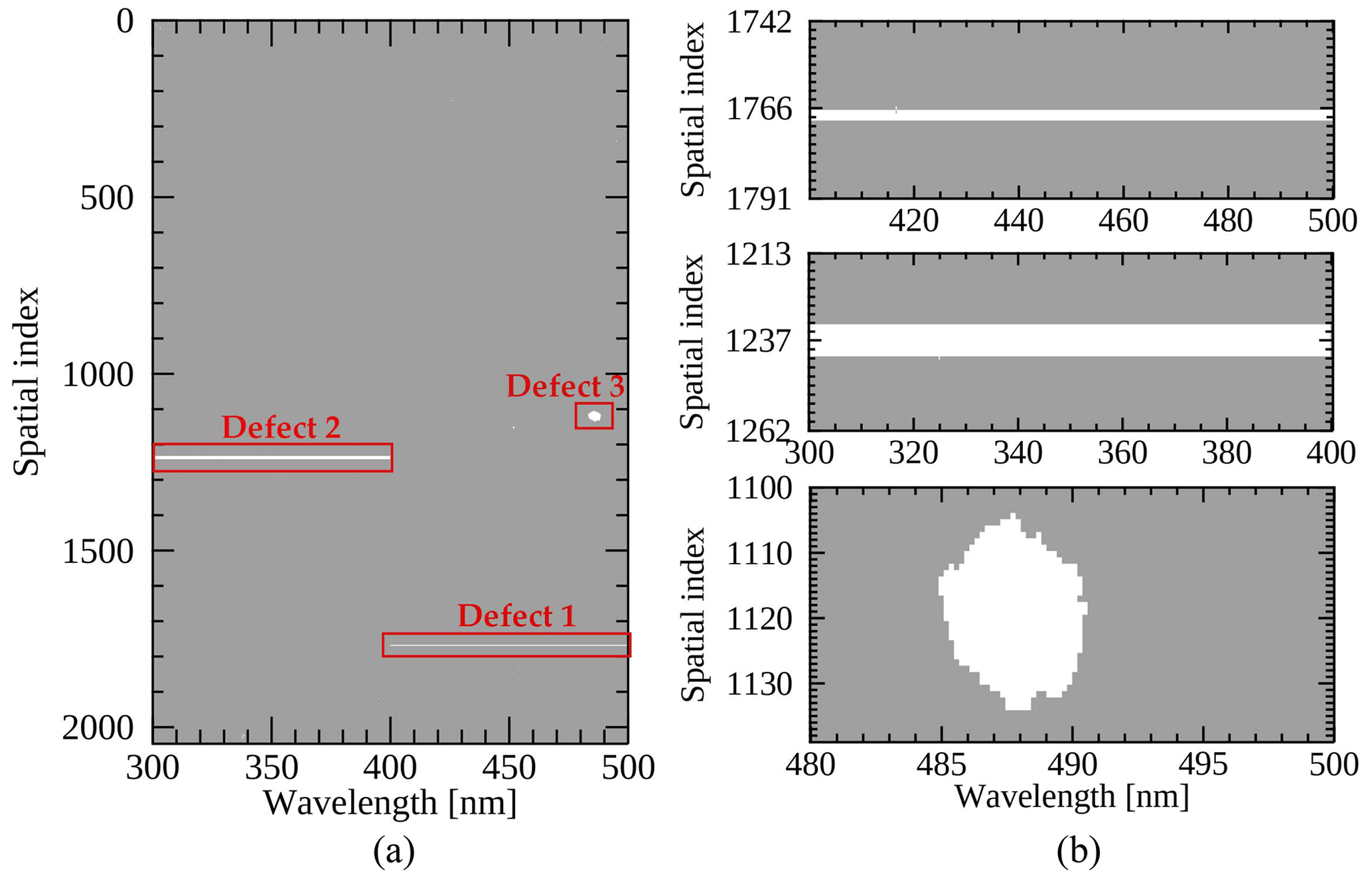
Figure 1The two-dimensional bad-pixel map (a) on the GEMS CCD detector along the spectral (x axis) and spatial direction (y axis) and (b) zooming in on the bad-pixel positions from top to bottom rows for Defects 1–3. Bad pixels are marked in white.
The interpolation error seriously affects Level 2 products for which the spectral fitting windows are overlapped with bad-pixel areas. For instance, cloud properties and aerosol effective height (AEH) of GEMS are retrieved from O2–O2 absorption bands around 477 nm (Choi et al., 2021; Kim et al., 2021) where the cluster of bad pixels is located (Defect 3). During the IOT, Defect 3 caused spatial discontinuity to the retrieved cloud and AEH distribution, which made the fitting window of the products moved to avoid bad-pixel effects. Ozone retrieval is also affected by Defect 2 (300–400 nm) as the spectral radiances within 300–380 nm are major ozone absorption lines in the UV–VIS spectral range (Bak et al., 2019). Even though spatially interpolated radiances are homogeneous with their surroundings (see Fig. 2), the spectral patterns are not properly reproduced with the operational method (spatial interpolation) causing distinct horizontal lines in the retrieved products (to be discussed in Sect. 3.2 2).
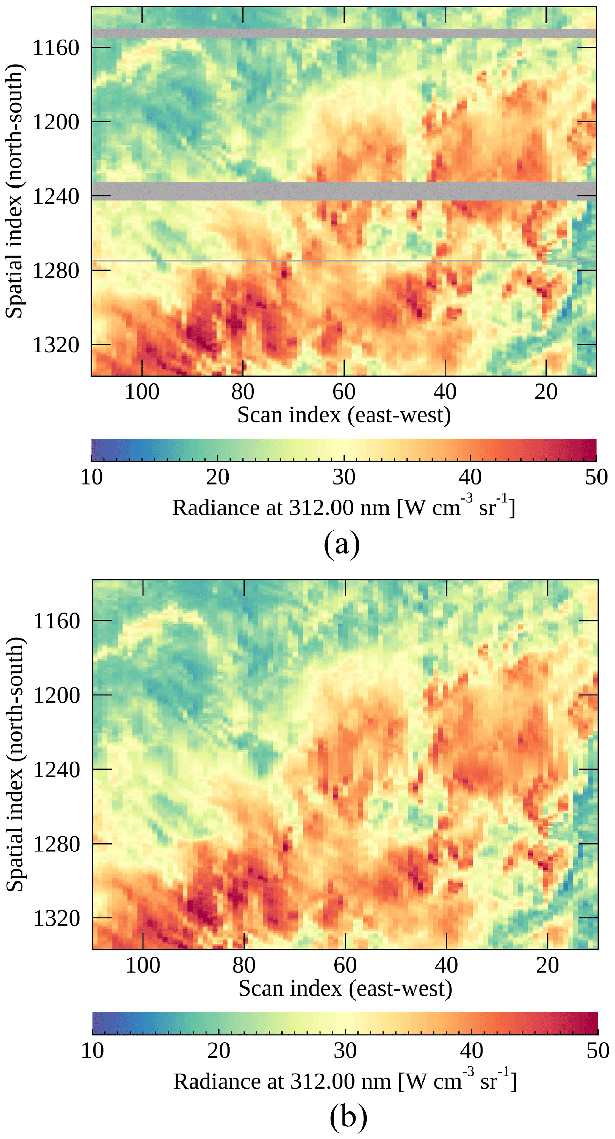
Figure 2Spatial distribution of GEMS radiances at 312 nm with bad pixels (a) marked in dark gray and (b) reproduced with spatial interpolation. The GEMS spectra were measured on 10 March 2021 (06:00 UTC).
2.2 Replacement approach
2.2.1 General description
Upwelling radiances are determined by the interactions of light with trace gases, aerosols and clouds in the atmosphere and surface reflection. Spectral replacement is based on the fact that radiances at different wavelengths for a scene have certain spectral relations (Liu et al., 2006; Wu et al., 2018) with which missing values in a spectrum could be reproduced. To investigate this, randomly collected GEMS spectra measured on defect-free pixels are used to establish the relations with the basic premise that neighboring pixels on the detector array (set to within 100 spatial indices) would have similar measurement characteristics.
Because it is highly possible that input radiances have redundant information, PCA is applied for dimensionality reduction to compress the input radiances to low-dimensional principal components (PCs). The strong linear relations among radiances in a spectrum are compressed to the first PC, which has the largest variance. The non-linear properties caused by atmospheric scattering, absorption, different optical paths and sensor noise are projected onto the subsequent PC subspaces. The PCA process is given by the following Eq. (1):
where Z, X and W represent the PC scores, input and PC matrix, respectively. The PC scores matrix (Z) is obtained by projecting the input to the PC subspaces with W, which is obtained by applying eigenvalue decomposition to the X. The subscripts n, λ and p indicate the dimension of matrix corresponding to the number of datasets, input wavelengths and the number of PCs, respectively.
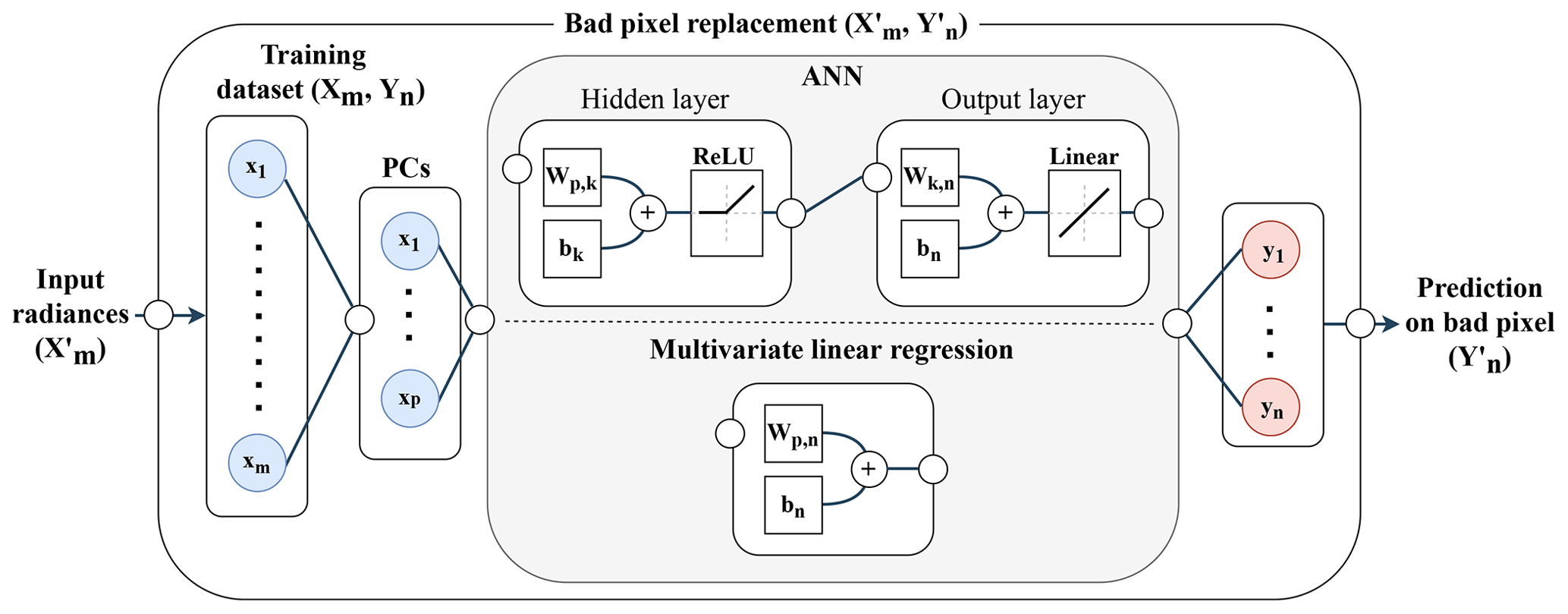
Figure 3Schematic chart of the training and bad-pixel replacement process. W and b represent weight and bias parameters in each layer. The subscripts m, n, p and k are equal to the spectral dimension of input and output parameters, the number of PCs, and the hidden nodes of the ANN model, respectively.
With the compressed data, multivariate linear regression (PCA-Linear) and ANN (PCA-ANN) models are trained to define the relations between input (Xm) and output (Yn) radiances in a spectrum. The PCA-ANN model is constructed with a simple feed-forward model with a hidden layer as described in Fig. 3. In the model optimization process, the PCA-ANN model with a hidden layer showed faster and more effective convergence of loss function than the models having multiple hidden layers. The PCA-Linear model adopts a simple linear model structure consisting of parameters such as weight and bias having the minimum mean squared error (MSE) between the regressed and measured radiances. After model optimization, bad pixels (, ) are replaced with reproduced radiances likely measured by the sensor.
2.2.2 Input–output and model optimization
For the model training, radiances in a spectrum are divided into input and output radiances based on the specified spectral ranges in Table 2. The spectral ranges of output radiances for Defects 1–3 are identical to each defective region, while the remaining part of a spectrum is the input radiances. The GEMS measurements randomly selected in a month (March 2021) are split into training and test data, which are used to update model parameters and to check for overfitting, respectively. The sampling process should be carefully done to avoid unstable training caused by oversampling of certain scenes (dark scenes in this case). The datasets for the models are interpolated at identical spectral grids in a pre-processing step and then are reversely interpolated onto its original spectral grids after the reproduction. Considering that the intrinsic information could be lost during the interpolation processes, finer spectral grids (0.1 nm) are adopted for the model to minimize interpolation errors by preserving radiances at more frequent intervals. The solar zenith angle (SZA) and viewing zenith angle (VZA) are key variables determining optical paths of upwelling and downwelling radiances and thus are used as input variables together with radiances. As described in Fig. 3, the activation function is the rectified linear unit (ReLU) in the hidden layer of the ANN model. The structure itself is not complicated, but it has multiple nodes in the input and output layers, which makes ReLU more competitive (Nwankpa et al., 2018). The hyperbolic tangent (tanh) and sigmoid function show poor results especially when the output parameters have lower variance making the optimization stuck at the average value and preventing the model from being updated.
Table 2Input and output (I/O) parameters for the training process of machine learning models and the optimized hyperparameter setting of the ANN model.

For the optimizer, Adaptive Moment Estimation (Adam) is used which shows stable results compared to stochastic gradient descent (SGD) and root mean square propagation (RMSProp) (Kingma and Ba, 2014). It is empirically found that SGD without gradient clipping tends to cause exploding gradients and RMSProp has difficulty reaching the global minima compared to Adam. Figure 4 presents the converging process of the PCA-ANN model for Defect 2 applying different optimizers with and without SZA and VZA conditions. The addition of angle conditions as input parameters speeds up the model convergence with smaller MSE because without it, the information would be implicitly elicited in the optimization process. The models with angle conditions converge at 44, 98 and 33 epochs for Adam, SGD and RMSProp, respectively. Adam converges at the smallest MSE, while SGD converges with the highest MSE. RMSProp presents unstable loss for validation data and converges with higher MSE compared to Adam.
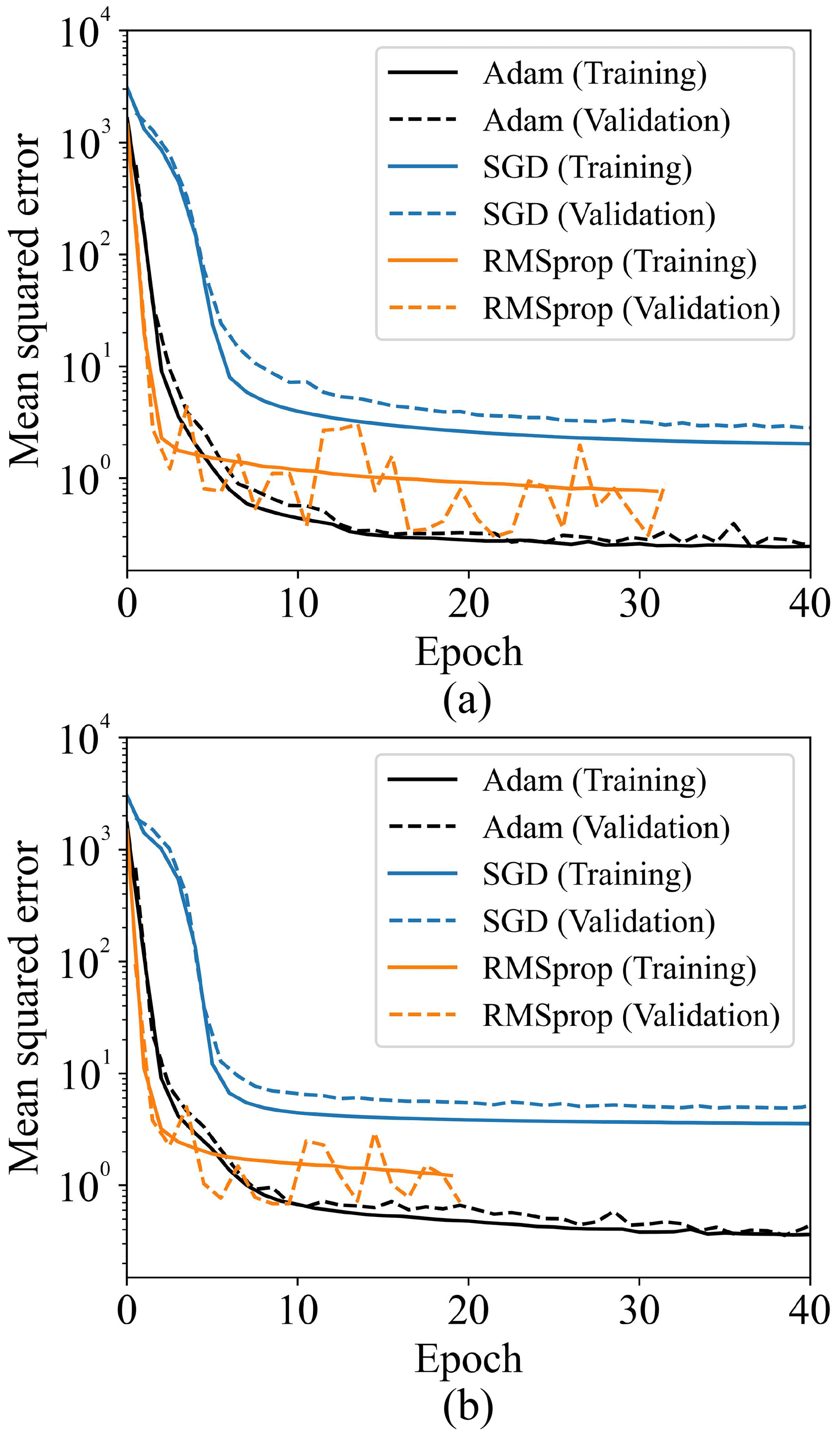
Figure 4Training and validation losses for Defect 2 (a) with and (b) without the angle conditions as input parameters with different optimizers such as Adam (black), SGD with the gradient clipping value of 0.5 (blue) and RMSProp (orange).
3.1 Model optimization
Figure 5 shows model optimization results for each model with the different number of PCs as the input nodes. Because the spectral range of output radiances differs for each defect region (Defects 1–3), model optimization is also separately performed. The spectral ranges of output radiances for Defects 1 and 2 are wider than that of Defect 3, which results in higher MSE. PCA-ANN seems to be unstable for Defect 1 showing overfitting which might be caused by unfiltered outliers in output radiances of GEMS at the wavelengths longer than 480 nm. Defect 2 contains ozone absorption lines which increase non-linearity between input and output radiances. Because of the strong non-linearity, PCA-ANN shows better performance than PCA-Linear for Defect 2. Defect 3 has the smallest number of output parameters in a narrow spectral gap, which causes strong correlation between input and output radiances as shown in Fig. 5c. In short, the optimized number of PCs is set to 90 for all defect regions when loss functions for both training and test data converge, with PCA-Linear for Defects 1 and 3 and the PCA-ANN model for Defect 2.
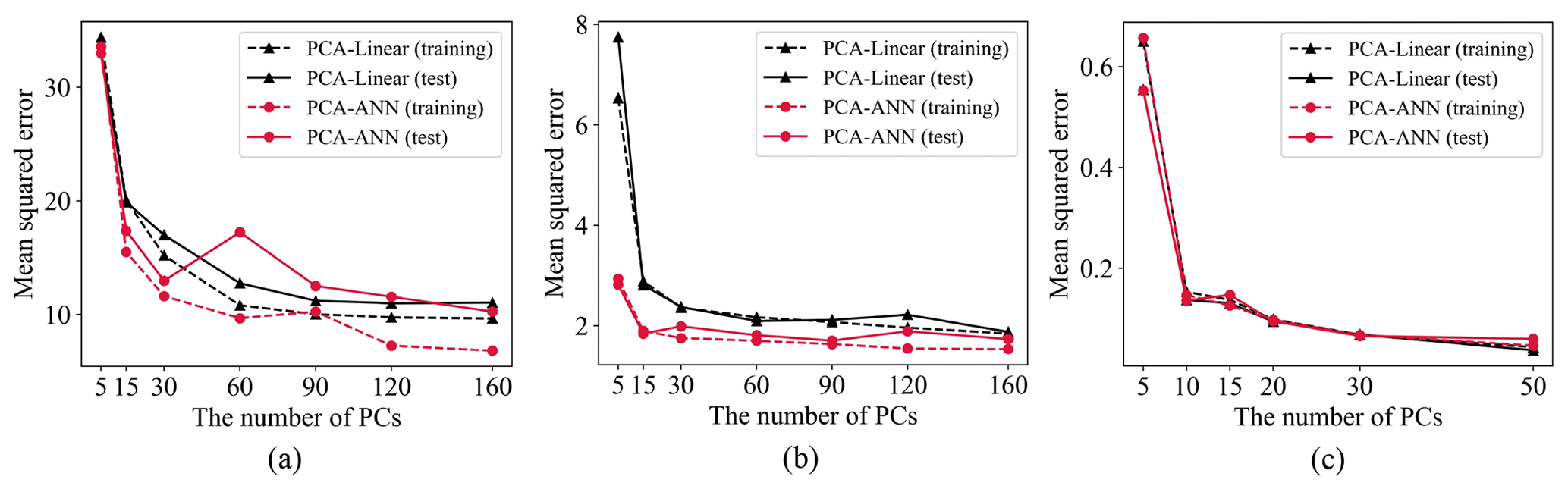
Figure 5Loss function with the different number of PCs of the PCA-ANN (red) and PCA-Linear (black) models for spectral replacement with training and test datasets for Defects 1–3 (a: Defect 1; b: Defect 2; c: Defect 3). The number of hidden nodes for ANN is double the number of PCs.

Figure 6Output radiances for Defect 1–3 with the average and NRMSE for (a) training and (b) test datasets measured in March 2021. The unit of NRMSE is percent.
The model performance is evaluated with training and test datasets specified in Table 2. Figure 6 presents mean and normalized root mean squared error (NRMSE) of the output radiances for both datasets. The NRMSE is a statistical indicator normalized by the mean radiance at each wavelength. Especially, the radiances in 400–500 nm provide insufficient information to properly represent ozone absorption features at the wavelengths shorter than 325 nm in Defect 2. Defect 1 also has higher errors around the edges of output spectral ranges where pixel saturation occurs. Defect 3 shows the smallest NRMSE of around 0.2 % because of strong linear relations between input and output radiances. The results show that it is possible to successfully reproduce spectral features at a narrower spectral range.
3.2 Evaluation
3.2.1 Spatial inspection
For quantitative evaluation, we investigated each defect area (Defects 1-3) and its surroundings where actual measurements regarded as “true” exist. The evaluation is made with the data measured on 10 March 2021 (06:00 UTC), which are excluded for the model training. Table 3 presents spectral ranges of Defects 1–3 and the target wavelengths for the analysis. Targeting the wavelengths helps analyze the exact spectral patterns.
Table 3The spectral range of Defects 1–3 and target wavelengths for the analysis. The third column presents GEMS retrieval products for which the fitting window is overlapped with Defects 1–3.

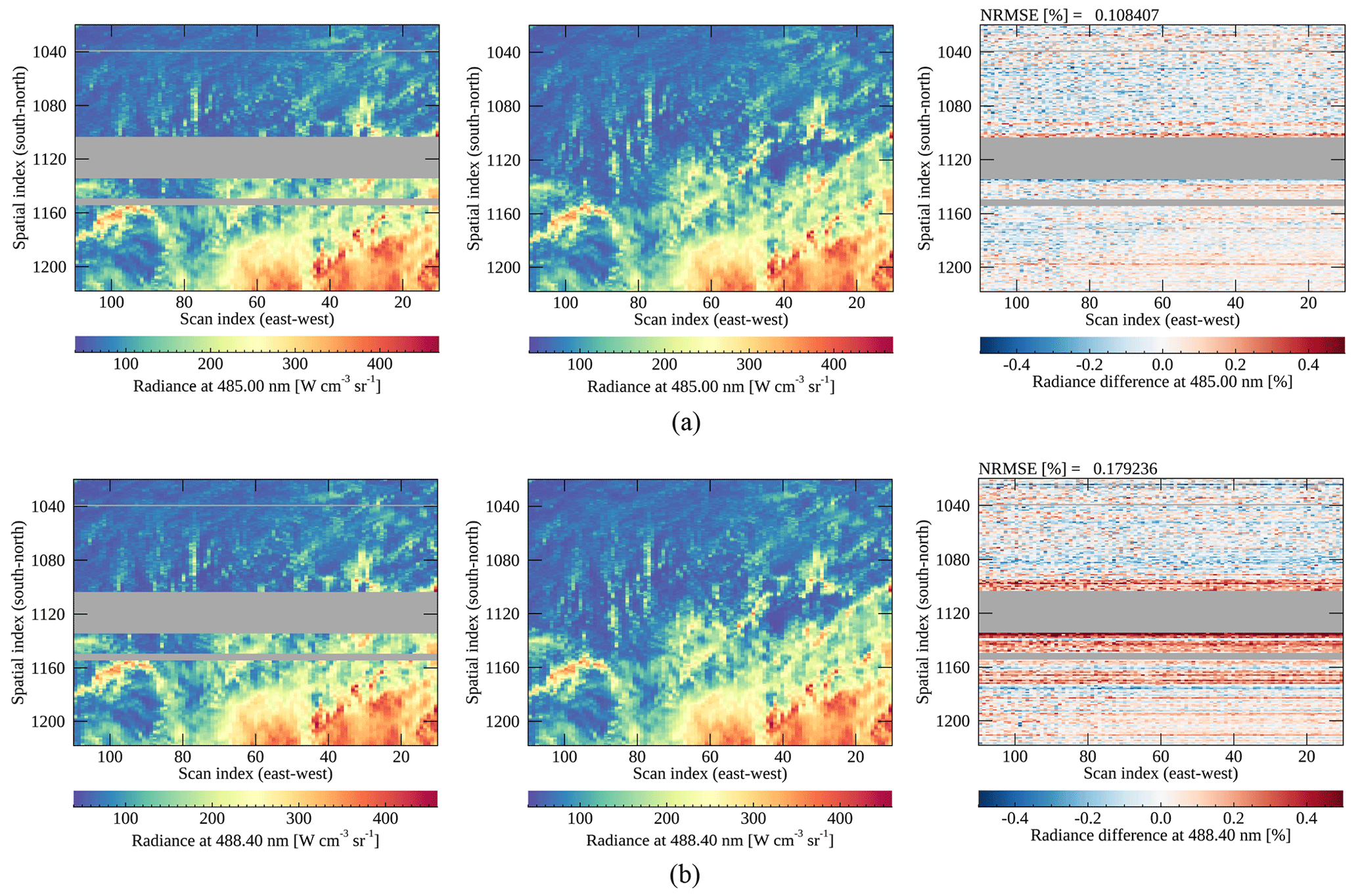
Figure 7Spatial distribution of GEMS, ML radiances and the differences (from the first to the third column) at the wavelengths presenting (a) the smallest and (b) the largest differences for the Defect 3 area. The difference is calculated between the ML and GEMS radiances and divided by the latter in percent. Bad pixels are marked in dark gray, and the color bar range for differences is ±0.5 %. The unit of NRMSE is percent divided by mean radiance.
The measured and reproduced radiances with machine learning methods are directly compared, which are hereafter referred to as GEMS radiances and ML radiances. In Figs. 7–9, each column shows GEMS, ML radiances and the differences, while the first and second rows show the radiances at the wavelengths showing the smallest and the largest differences, respectively. Figure 7 shows the comparison results of the Defect 3 area, which represents the best performance among the three defect areas. The differences in Fig. 7 are within the range of ±0.5 % because the spectral gap of Defect 3 is narrower than the counterparts of Defects 1–2. For Defect 3, there is no distinct scene dependence over the output wavelengths and the differences show noise-like features originating from instrument artifacts. One thing to be noted is that the results presented here are calculated at the finer spectral grids of 0.1 nm before being interpolated to the original spectral grids. After the interpolation, the differences especially at strong peaks in a spectrum could increases by 0.5 % for Fig. 7b.
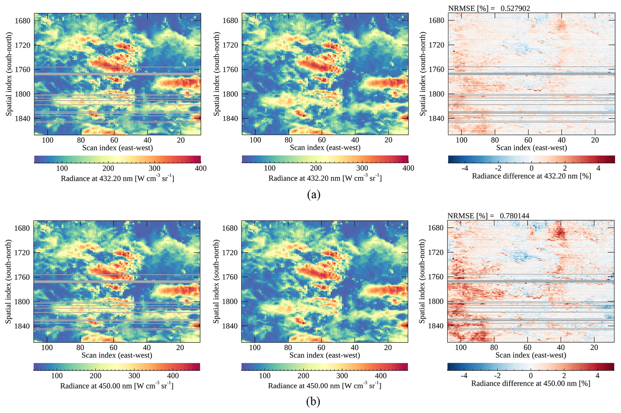
Figure 8Same as Fig. 7 for the Defect 1 area with the color bar range for differences within ±5 %.
Figure 8 shows the Defect 1 area where differences between GEMS and ML radiances are within about 5 %. It shows that dark targets (clear sky with low radiance) show a positive difference, while bright targets (mostly clouds with high radiance) show the opposite. The tendency is also found on the other dates for different angle conditions. It seems the applied machine learning model (PCA-Linear) might have its limitation in describing the non-linear relations of angle conditions, scene properties and radiances causing the difference of about 5 %.
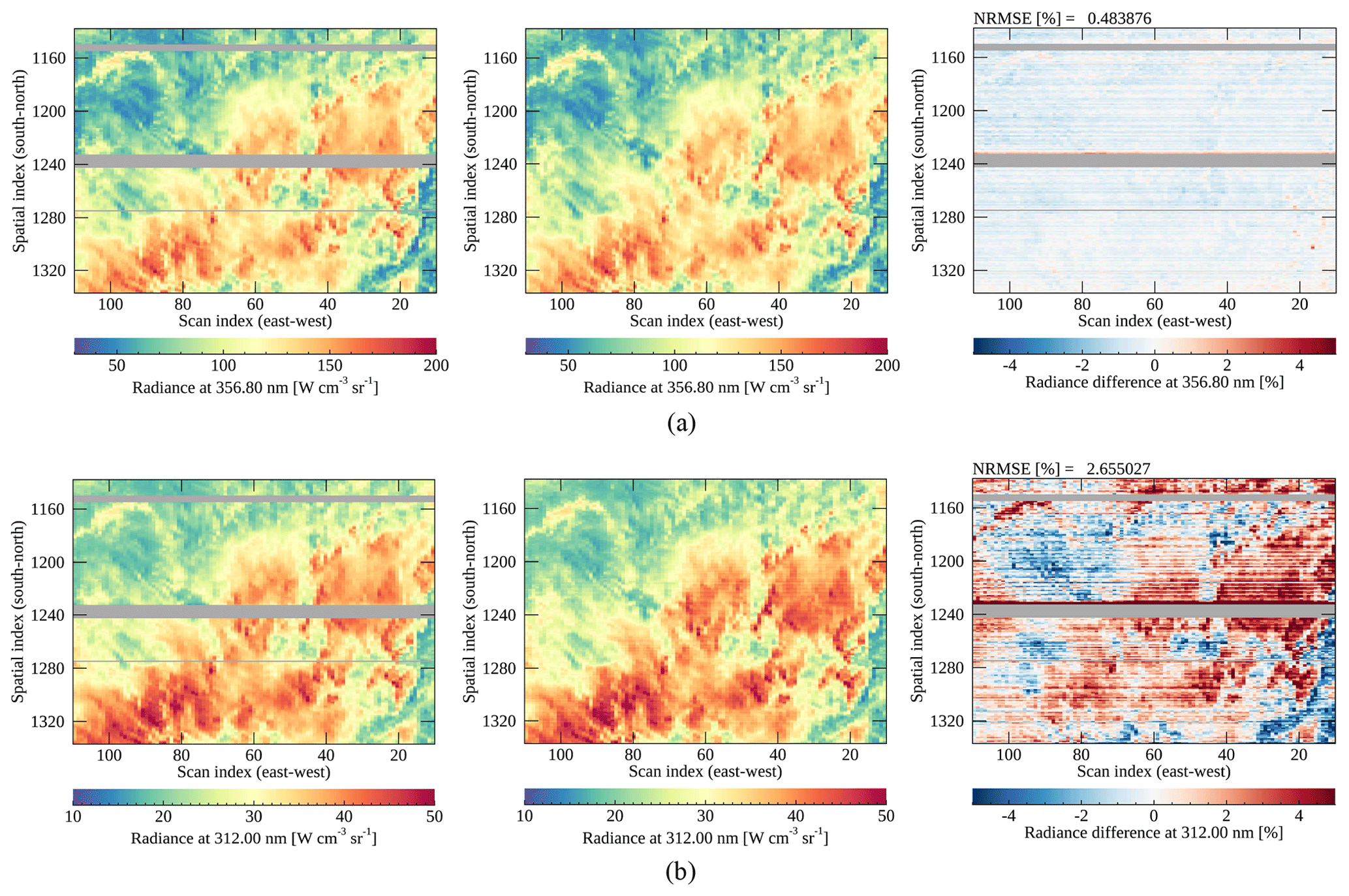
Figure 9Same as Fig. 8 for the Defect 2 area with the color bar range for differences within ±5 %.
For the Defect 2 area, the information from radiances at the wavelengths longer than 400 nm is insufficient to effectively reproduce the spectral features at shorter wavelengths (consistent results with Fig. 6). Both Defects 2–3 have the output spectral ranges of about 100 nm, but it seems the output radiances near 300 nm for Defect 2 need more information. In particular, the stripping features found in Fig. 9b are more significant at 312 nm for the ML radiances compared to Fig. 9a. The stripping features seem to be added during the reproducing process especially for shorter wavelengths, and the reason is still unclear. We suspect that unpredictable noises from the instrument would cause the features, and it seems more distinguishable in low signals. The scene dependence found in Fig. 8 is also dominant in Fig. 9 at shorter wavelengths but with the opposite tendency. It is also shown that some areas undetected as bad pixels cause big differences over the areas close to the spatial index of 1240 in Fig. 9.
3.2.2 PCA-based analysis
To further characterize the reproduced spectral patterns, we apply PCA to GEMS radiances collected within each area in Figs. 7–9 at the target wavelengths (see Table 3). With PCA, various spectral patterns are compressed to PC scores. If a spectrum has disparate spectral patterns, the PC scores would have distinct values compared to the PC scores of defect-free spectra. Figure 10 shows the PC scores of GEMS and ML radiances projected with the identical eigenvector matrix (corresponding to X in Eq. 1) constructed with GEMS radiances. The Defect 3 area is presented for the visual inspection with the second PC scores because the first PCs mostly represent mean radiances. The radiances reproduced with spatial interpolation on the bad-pixel area show disparate values as shown in Fig. 10a. The ML radiances in Fig. 10b show spatially homogeneous PC scores on the contrary because the machine learning methods properly reproduce dominant spectral patterns.
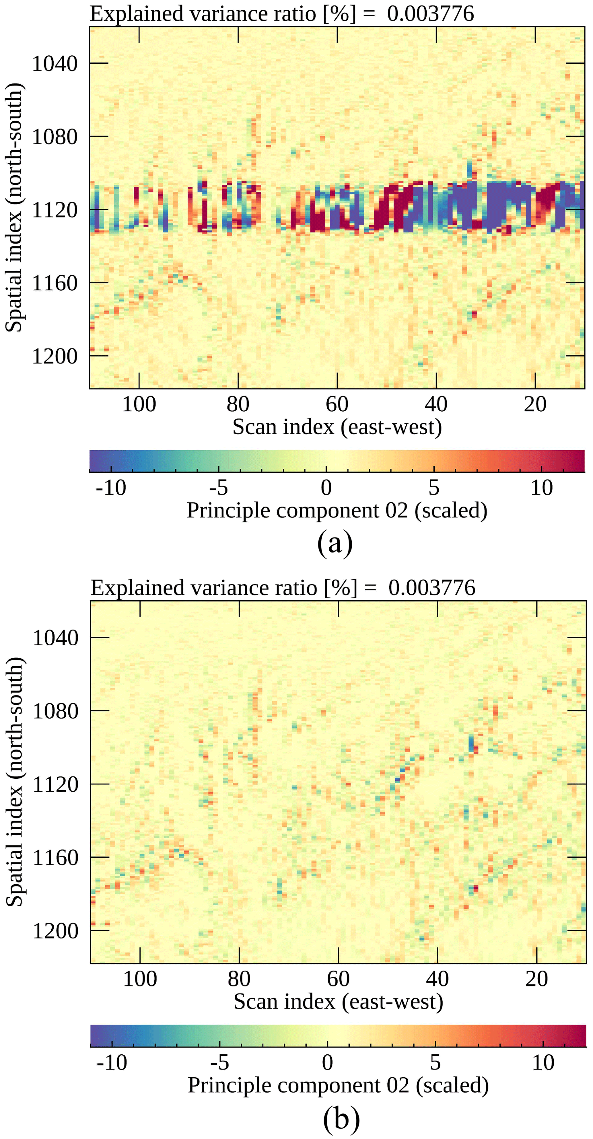
Figure 10The second PC scores of (a) GEMS radiances and (b) ML radiances on the target area for Defect 3. The PC is scaled for clarity of presentation.
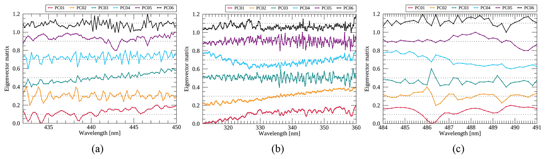
Figure 11Eigenvector of the first six PCs applied to GEMS radiances for the target wavelengths of (a) Defects 1, (b) Defect 2 and (c) Defect 3. All eigenvectors are scaled (min–max scaling) and shifted for clarity of presentation.
The dominant spectral patterns for each PC are presented in Fig. 11 with the eigenvector matrix constructed from GEMS radiances for the specified target wavelengths in Table 3. Each color indicates the eigenvector for the first six PCs contributing to total radiances at each wavelength. Li et al. (2015) verified that the leading PCs (shorter than 360 nm) mainly represent dominant absorption and surface properties, while the trailing PCs are associated with instrument artifacts and unresolved spectral features, as similarly shown in Fig. 11.
Table 4Correlation coefficients (Corr.) of PC scores of GEMS and ML radiances and the EVR of GEMS radiances for each target region in Figs. 8–10 excepting bad-pixel area.
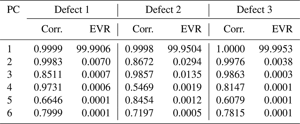
As presented in Table 4, comparing PC scores provides qualitative information on the effectiveness of the suggested method. The results show that the mean spectral pattern (the first PC) and dominant patterns could be reproduced with sufficient information. However, other spectral features such as the third PC for Defect 1 or the second PC for Defect 2 show insufficient information available from input radiances. As shown with the explained variance ratio (EVR), each PC except the first one may contribute to a small extent to total radiances. However, it could be enough to determine subtle spectral patterns, which are important for retrieval processes. The effectiveness of spectral replacement could be glimpsed in the results, which will be discussed further in the following section with retrieval results.
3.3 Level 2 retrieval results
3.3.1 Cloud and ozone retrieval
In the previous section, the overall prediction error with the suggested method is about 5 % for radiances except for ozone absorption lines. The next question is whether the reproduced spectral features are applicable to retrieval processes. Even if the trained models accurately reproduce radiances at each wavelength, the Level 2 retrieval could be unsuccessful if non-linear relations are too elusive to be properly emulated with the model. To prove this, we performed the cloud retrieval with the fitting window in 460.2–490.0 nm containing bad pixels. The replaced radiances at O2–O2 absorption lines related to Defect 3 have the smallest error of 0.5 %, and the retrieval is quite successful. Figure 12 presents cloud centroid pressure retrieved with ML and GEMS spectra by zooming in on defect-free areas to analyze cloud distribution. The difference in cloud centroid pressure between Fig. 12a and b is about 1 % on average, while the cloud properties of ML spectra have weak stripping features. The spectral range of Defect 3 is very narrow within the fitting window, and thus the replacement errors could be small enough not to cause additional retrieval errors.

Figure 12Spatial distribution of cloud centroid pressure retrieved with (a) GEMS and (b) ML radiances zooming in on a certain area presented in Fig. 7. The GEMS spectra were measured on 10 March 2021 (06:00 UTC).
Ozone retrieval results are presented in this section. Figure 13 shows total ozone column density including bad pixels and defect-free areas as presented in Fig. 9. The ozone properties retrieved with measured GEMS spectra show distinct spatial discontinuity over the bad-pixel area (see Fig. 13a), while the discontinuity is somewhat reduced with ML spectra in Fig. 13b. However, the retrieved properties show different spatial distribution patterns even for the defect-free areas. It seems the ozone properties are underestimated especially for higher radiances in Fig. 13b, and the stripping features found in Fig. 9 also exist in Fig. 13b. The SZA and VZA as input parameters of the PCA-ANN model provide important information because ozone retrievals with replaced radiances without the angle information show unrealistic features with much higher variance (not shown). In short, the ozone properties retrieved with the ML spectra can present approximate spatial patterns within the reasonable ranges but with high uncertainty within about 8 %–10 %.
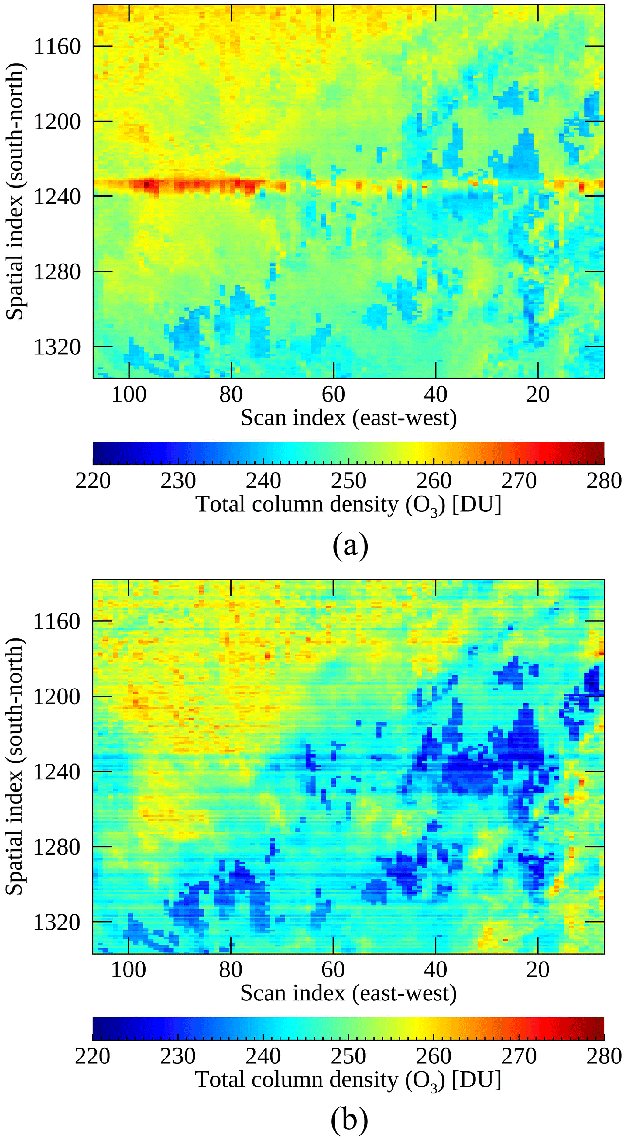
Figure 13Spatial distribution of total ozone column density retrieved with (a) GEMS and (b) ML radiances presented in Fig. 9. The GEMS spectra were measured on 10 March 2021 (06:00 UTC).
3.3.2 Cause analysis for further application
The high uncertainty in ozone retrieval is attributed to the lack of information in the input data or insufficient model optimization because the inputs (400–500 nm) may have deficient information. To clarify this and investigate further, we targeted ozone absorption lines in 312–360 nm and Fraunhofer lines in 390–400 nm for the replacement with different input cases. In the Fraunhofer lines, the Ring effect caused by rotational Raman scattering can be found over two radiance peaks and is generally known to be very small and largely affected by the existence of clouds (Joiner et al., 1995). It is expected the analysis can give clear evidence on whether the small scattering features could be reproduced with machine learning for different input wavelengths. For the analysis, the PCA-ANN model is trained for each input case, with defect-free measurements in March 2021 (around 80 000 spectra after bad-pixel masking and the elimination of saturation pixels).
Figure 14 presents mean absolute errors in reproduced radiances at ozone absorption and Fraunhofer lines with four different input conditions: (1–2) including each near side (within 20 nm) from the output spectral regions (A or B for the left and the right side, respectively); (3) including both near sides of wavelengths (A and B); and (4) all wavelengths in 300–500 nm except for A, B and the output spectral region. Each input case is plotted in Fig. 14 as red, sky blue, blue and black lines. Results show that prediction errors increase at the spectral peaks and overall error patterns differ with different input conditions. As assumed, the errors are higher with the input spectral bands farther from the output spectral region. Figure 14a clearly shows that insufficient information from the input data may cause large errors for radiances at shorter wavelengths related to the ozone retrieval. Figure 14b also presents that each input case has a different level of information, which could determine the accuracy of spectral replacement especially for the weak scattering features.
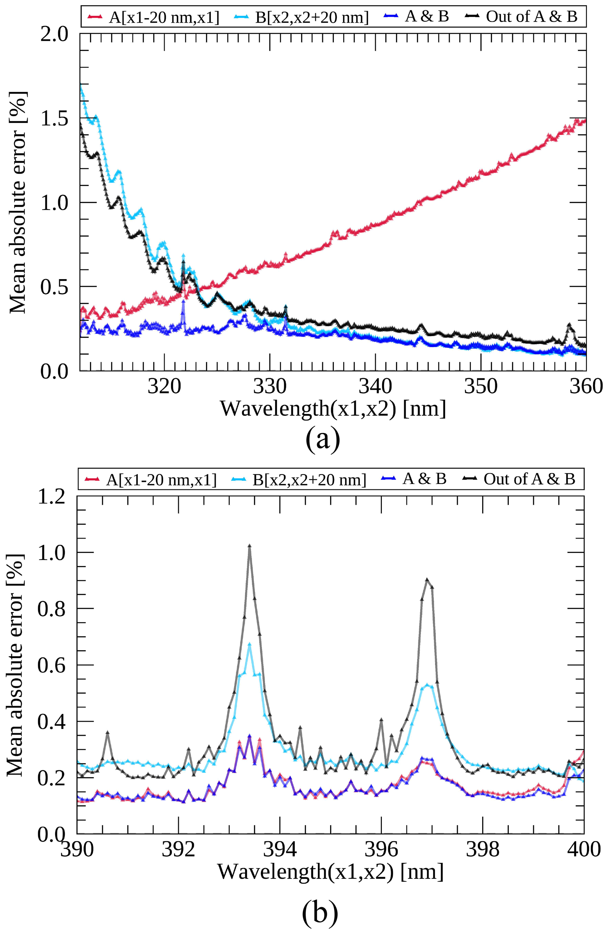
Figure 14Mean absolute errors between the reproduced and measured radiances at (a) ozone absorption and (b) Fraunhofer lines with different input cases. The x1 and x2 in the legend indicate the wavelengths at the boundary of output spectral bands, respectively. The absolute error is calculated between the ML and GEMS radiances and divided by the latter in percent.
Figure 15 presents a closer inspection by dividing spectra into four groups depending on the scene brightness. Different scenes could have different error levels which could be ignored in the averaged values in Fig. 14. The analysis is performed with the spectra reproduced with the input conditions showing the smallest (blue lines) errors in Fig. 14. Figure 15 shows that the PCA-ANN model reproduces dominant spectral features with an error of 0.4 % for all scenes with the best input condition. However, the difference increases with darker scenes (weak signals), which indicates low signals would be less predictable even with the information extracted from the very close wavelengths. It could be a limitation because radiances with small signals mostly have meaningful information for trace gases (clear-sky) in the UV–VIS spectral region.
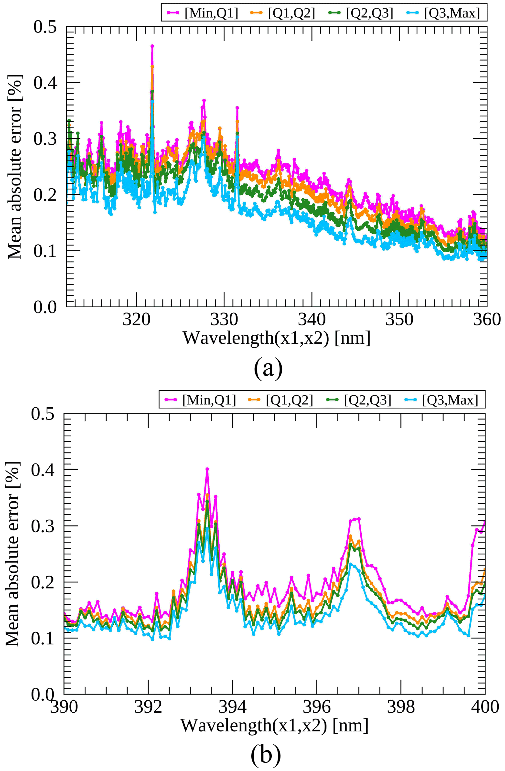
Figure 15Mean absolute errors between the reproduced and measured radiances at (a) ozone absorption and (b) Fraunhofer lines with the input case showing the smallest errors in Fig. 14. The Q1, Q2 and Q3 represent the first, second and third quartile, and each color indicates the average in the range of each quartile. The x1 and x2 indicate wavelengths at the boundary of output spectral bands and the absolute error is calculated between the ML and GEMS radiances and divided by the latter in percent.
In this section, the reproduced absorption or scattering lines are compared with different input conditions. The suggested method (PCA-ANN) could be quite effective when the input spectral ranges are closer to the target wavelengths to be reproduced. However, it is not necessarily true that the wider the input spectral range is, the more accurate the replacement becomes. If input spectral ranges have some calibration issues (e.g., stray light or saturation) or provide conflicting features with other input spectral bands as shown in Fig. 14a, the reproduced spectrum would have inconsistent features causing higher error. In summary, the suggested method accurately predicts the overall magnitude of a spectrum, but reproducing finer spectral features with high accuracy would need more information especially for low signals or strong absorption lines. At least, the input and output spectral regions should be close enough to reduce the spectral error up to 0.5 %, the uncertainty in the reproduced spectra at O2–O2 absorption lines presenting successful cloud retrieval results.
GEMS is an environmental sensor measuring hyperspectral radiances from 300 to 500 nm in the Asia–Pacific region for timely atmospheric monitoring. During the IOT of GEMS, we found that bad pixels on the detector array are not properly replaced with spatial interpolation, the current operational method. It is clear that when the bad-pixel area is too large, the spatial interpolation tends to cause a high interpolation error especially for a scene having large spatial inhomogeneity (i.e., cloud edges). The high interpolation error causes horizontal discontinuity at a certain latitude in the retrieval of Level 2 products.
For this reason, in this study, we more focus on improving the erroneous radiances to check whether the issue could be more efficiently resolved for both radiances and retrieved properties. This study suggests machine learning methods (PCA-ANN and PCA-Linear) to fill in various spectral gaps denoted as Defects 1–3 by investigating how much information could be obtained to reproduce spectral features without any additional information. The basic assumption of this approach is that radiances of a spectrum have strong linear and non-linear relations, which could be emulated with the ANN and multivariate linear regression. The spectral range of output radiances is set to the wavelengths of bad pixels, while the input radiances correspond to the remaining part of a spectrum for Defects 1–3.
In the results, the PCA-Linear model presents smaller prediction errors for the defective regions which have strong linear relations between input and output radiances (Defect 1) or a narrower spectral gap (Defect 3). When applying the reproduced spectra in Defect 3 to the cloud retrieval, cloud centroid pressure is successfully retrieved with an error of 1 % on average. This is because the output spectral range of Defect 3 is comparably narrower and thus the input wavelengths provide enough information to reproduce exact spectral features. The PCA-ANN model is better for the output radiances having strong non-linear relations (Defect 2). Dominant spectral patterns and the overall magnitude of spectra could be successfully reproduced mostly with an error of 5 % except for ozone absorption lines. When applying the reproduced spectra to the ozone retrieval, however, we can obtain the spatial patterns of total ozone column density with higher uncertainty within about 8 %.
Further investigation reproducing Fraunhofer lines and ozone absorption lines helps conclude the benefits and limitations of the approach as follows:
-
The closer the input and output wavelengths are, the smaller the reproduction error becomes. This is because radiances at adjacent wavelengths could contain more information valid for the replacement. Even though the condition is not fulfilled, approximate spatial patterns could be obtained but with low accuracy for both radiances and retrieval properties.
-
The input radiances should be carefully selected because machine learning models (especially ANN) are vulnerable to outliers or erroneous input radiances. If one adopts more complex models, the importance of the selection would increase.
-
Errors coming from instrument artifacts such as the stripping feature could be propagated with the method as it seems the feature is not properly emulated in the model.
-
Finally, low radiances could have higher uncertainty even when using the spectral information as much as possible. GEMS is an environmental sensor and thus may provide useful information with clear-sky conditions. Considering this, additional information would be needed if one pursues very high retrieval accuracy with the replaced spectra. In this regard, combining the external information together with the spectral components would be the next step to develop the approach. Since the research adopts very simple machine learning models, it also can be updated further.
Considering that the number of bad pixels would increase in operation as it did in the Ozone Mapping and Profiler Suite (OMPS) (Seftor et al., 2014), an efficient way of replacing bad pixels would be necessary for the long-term operation of GEMS. It is also highly possible that an unexpected issue could occur such as the row anomaly of the Ozone Monitoring Instrument (OMI) (Schenkeveld et al., 2017). The ultimate goal of this research is to increase the usefulness of GEMS data for a longer time period, at least for a designed lifetime of 10 years. The current work verifies that the gap filling (in Level 1) with certain spectral conditions shows quite reliable results even with the limitations for the strong absorption bands, which is natural and provides the reason why we need observation data over such spectral bands. However, we also anticipate that with the accumulation of measurements along with auxiliary data and an improved non-linear algorithm, the limitation could be improved in future study. For this reason, this paper provides the basis for further applicability of the method by evaluating the efficiency of machine learning methods to reproduce hyperspectral data especially in the UV–VIS spectral range.
The neural network presented in this study is implemented with TensorFlow (https://www.tensorflow.org/install/, last access: 12 January 2023; TensorFlow, 2023), a high-level Application Programming Interface (API) written in Python. TensorFlow is an open-source library provided by Google Colab. The machine learning codes are available on request from the corresponding author.
The GEMS Level 1C data are available on request from the National Institute of Environmental Research (NIER) – Environmental Satellite Center (ESC). The GEMS Level 2 products and the algorithm theoretical basis documents (ATBDs) can be accessed through the following web page (https://nesc.nier.go.kr/product/view/, last access: 12 January 2023; NIER-ESC, 2023).
MHA conceptualized and supervised the study; YL conducted the research, performed the experiments and prepared the paper; MK contributed to the editing of the paper and developing methodology. ME contributed to the pre-processing of raw data.
The contact author has declared that none of the authors has any competing interests.
Publisher’s note: Copernicus Publications remains neutral with regard to jurisdictional claims in published maps and institutional affiliations.
This article is part of the special issue “GEMS: first year in operation (AMT/ACP inter-journal SI)”. It is not associated with a conference.
We wish to express our gratitude to Glen Jaross and the anonymous reviewer for their valuable comments to greatly improve the quality of this research. We also thank Kang-Hyeon Baek (Pusan National University) and Gyuyeon Kim (Ewha Womans University) for the assistance in retrieving Level 2 data for this study. The authors acknowledge the contribution of the NIER–ESC for providing GEMS Level 0-1C data.
This research has been supported by the Basic Science Research Program through the National Research Foundation of Korea (NRF) funded by the Ministry of Education (grant no. 2018R1A6A1A08025520).
This paper was edited by Jhoon Kim and reviewed by Glen Jaross and one anonymous referee.
Bajorski, P.: Statistical inference in PCA for hyperspectral images, IEEE J. Sel. Top. Signa., 5, 438–445, https://doi.org/10.1109/JSTSP.2011.2105244, 2011.
Bak, J., Baek, K.-H., Kim, J.-H., Liu, X., Kim, J., and Chance, K.: Cross-evaluation of GEMS tropospheric ozone retrieval performance using OMI data and the use of an ozonesonde dataset over East Asia for validation, Atmos. Meas. Tech., 12, 5201–5215, https://doi.org/10.5194/amt-12-5201-2019, 2019.
Boersma, K. F., Eskes, H. J., and Brinksma, E. J.: Error analysis for tropospheric NO2 retrieval from space, J. Geophys. Res.-Atmos., 109, D04311, https://doi.org/10.1029/2003jd003962, 2004.
Bovensmann, H., Burrows, J. P., Buchwitz, M., Frerick, J., Noël, S., Rozanov, V. v., Chance, K. V., and Goede, A. P. H.: SCIAMACHY: Mission objectives and measurement modes, J. Atmos. Sci., 56, 127–150, https://doi.org/10.1175/1520-0469(1999)056<0127:SMOAMM>2.0.CO;2, 1999.
Choi, H., Liu, X., Gonzalez Abad, G., Seo, J., Lee, K.-M., and Kim, J.: A Fast Retrieval of Cloud Parameters Using a Triplet of Wavelengths of Oxygen Dimer Band around 477 nm, Remote Sens.-Basel, 13, 152, https://doi.org/10.3390/rs13010152, 2021.
Cybenko, G.: Approximation by superpositions of a sigmoidal function, Math. Control Signal., 2, 303–314, https://doi.org/10.1007/BF02551274, 1989.
Fang, H., Liang, S., Townshend, J. R., and Dickinson, R. E.: Spatially and temporally continuous LAI data sets based on an integrated filtering method: Examples from North America, Remote Sens. Environ., 112, 75–93, https://doi.org/10.1016/J.RSE.2006.07.026, 2008.
Fischer, A. D., Downes, T. V., and Leathers, R.: Median spectral-spatial bad pixel identification and replacement for hyperspectral SWIR sensors, in: Proceedings of SPIE – Algorithms and Technologies for Multispectral, Hyperspectral, and Ultraspectral Imagery XII, 65651E, https://doi.org/10.1117/12.720050, 2007.
Gewali, U. B., Monteiro, S. T., and Saber, E.: Machine learning based hyperspectral image analysis: A survey, arXiv [preprint], https://doi.org/10.48550/arXiv.1802.08701, 23 February 2018.
Goetz, A. F. H., Vane, G., Solomon, J. E., and Rock, B. N.: Imaging spectrometry for earth remote sensing, Science, 228, 1147–1153, https://doi.org/10.1126/science.228.4704.1147, 1985.
Guo, L., Lei, L., Zeng, Z. C., Zou, P., Liu, D., and Zhang, B.: Evaluation of spatio-temporal variogram models for mapping Xco2 using satellite observations: A case study in China, IEEE J. Sel. Top. Appl., 8, 376–385, https://doi.org/10.1109/JSTARS.2014.2363019, 2015.
Han, T., Goodenough, D. G., Dyk, A., and Love, J.: Detection and correction of abnormal pixels in hyperion images, Int. Geosci. Remote Se., 3, 1327–1330, https://doi.org/10.1109/IGARSS.2002.1026105, 2002.
Hedelt, P., Efremenko, D. S., Loyola, D. G., Spurr, R., and Clarisse, L.: Sulfur dioxide layer height retrieval from Sentinel-5 Precursor/TROPOMI using FP_ILM, Atmos. Meas. Tech., 12, 5503–5517, https://doi.org/10.5194/amt-12-5503-2019, 2019.
Horler, D. N. and Ahern, F. J.: Forestry information content of thematic mapper data, Int. J. Remote Sens., 7, 405–428, https://doi.org/10.1080/01431168608954695, 1986.
Hornik, K., Stinchcombe, M., and White, H.: Multilayer feedforward networks are universal approximators, Neural Networks, 2, 359–366, https://doi.org/10.1016/0893-6080(89)90020-8, 1989.
Howell, S. B.: CCD imaging, in: Handbook of CCD Astronomy, Cambridge University Press, Cambridge, 66–101, https://doi.org/10.1017/CBO9780511807909.006, 2006.
Joiner, J., Bhartia, P. K., Cebula, R. P., Hilsenrath, E., McPeters, R. D., and Park, H.: Rotational Raman scattering (Ring effect) in satellite backscatter ultraviolet measurements, Appl. Optics, 34, 4513, https://doi.org/10.1364/AO.34.004513, 1995.
Joiner, J., Yoshida, Y., Guanter, L., and Middleton, E. M.: New methods for the retrieval of chlorophyll red fluorescence from hyperspectral satellite instruments: simulations and application to GOME-2 and SCIAMACHY, Atmos. Meas. Tech., 9, 3939–3967, https://doi.org/10.5194/amt-9-3939-2016, 2016.
Kang, M., Ahn, M. H., Liu, X., Jeong, U., and Kim, J.: Spectral calibration algorithm for the geostationary environment monitoring spectrometer (Gems), Remote Sens.-Basel, 12, 1–17, https://doi.org/10.3390/rs12172846, 2020.
Kang, M., Ahn, M. H., Ko, D. H., Kim, J., Nicks, D., Eo, M., Lee, Y., Moon, K. J., and Lee, D. W.: Characteristics of the Spectral Response Function of Geostationary Environment Monitoring Spectrometer Analyzed by Ground and In-Orbit Measurements, IEEE T. Geosci. Remote, 60, 1–16, https://doi.org/10.1109/TGRS.2021.3091677, 2022.
Katzfuss, M. and Cressie, N.: Spatio-temporal smoothing and EM estimation for massive remote-sensing data sets, J. Time Ser. Anal., 32, 430–446, https://doi.org/10.1111/J.1467-9892.2011.00732.X, 2011.
Kieffer, H. H.: Detection and correction of bad pixels in hyperspectral sensors, in: Proceedings of SPIE – Hyperspectrel Remote Sensing and Applications, 2821, https://doi.org/10.1117/12.257162, 1996.
Kim, G., Choi, Y. S., Park, S. S., and Kim, J.: Effect of solar zenith angle on satellite cloud retrievals based on O2–O2 absorption band, Int. J. Remote Sens., 42, 4224–4240, https://doi.org/10.1080/01431161.2021.1890267, 2021.
Kim, J., Jeong, U., Ahn, M. H., Kim, J. H., Park, R. J., Lee, H., Song, C. H., Choi, Y. S., Lee, K. H., Yoo, J. M., Jeong, M. J., Park, S. K., Lee, K. M., Song, C. K., Kim, S. W., Kim, Y. J., Kim, S. W., Kim, M., Go, S., Liu, X., Chance, K., Miller, C. C., Al-Saadi, J., Veihelmann, B., Bhartia, P. K., Torres, O., Abad, G. G., Haffner, D. P., Ko, D. H., Lee, S. H., Woo, J. H., Chong, H., Park, S. S., Nicks, D., Choi, W. J., Moon, K. J., Cho, A., Yoon, J., Kim, S. kyun, Hong, H., Lee, K., Lee, H., Lee, S., Choi, M., Veefkind, P., Levelt, P. F., Edwards, D. P., Kang, M., Eo, M., Bak, J., Baek, K., Kwon, H. A., Yang, J., Park, J., Han, K. M., Kim, B. R., Shin, H. W., Choi, H., Lee, E., Chong, J., Cha, Y., Koo, J. H., Irie, H., Hayashida, S., Kasai, Y., Kanaya, Y., Liu, C., Lin, J., Crawford, J. H., Carmichael, G. R., Newchurch, M. J., Lefer, B. L., Herman, J. R., Swap, R. J., Lau, A. K. H., Kurosu, T. P., Jaross, G., Ahlers, B., Dobber, M., McElroy, C. T., and Choi, Y.: New era of air quality monitoring from space: Geostationary environment monitoring spectrometer (GEMS), B. Am. Meteorol. Soc., 101, E1–E22, https://doi.org/10.1175/BAMS-D-18-0013.1, 2020.
Kingma, D. P. and Ba, J. L.: Adam: A method for stochastic optimization, arXiv [preprint], https://doi.org/10.48550/arXiv.1412.6980, 22 December 2014.
Le, T., Liu, C., Yao, B., Natraj, V., and Yung, Y. L.: Application of machine learning to hyperspectral radiative transfer simulations, J. Quant. Spectrosc. Ra., 246, 106928, https://doi.org/10.1016/j.jqsrt.2020.106928, 2020.
Lee, Y., Ahn, M. H., and Kang, M.: The new potential of deep convective clouds as a calibration target for a geostationary UV/VIS hyperspectral spectrometer, Remote Sens.-Basel, 12, 446, https://doi.org/10.3390/rs12030446, 2020.
Li, C., Joiner, J., Krotkov, N. A., and Bhartia, P. K.: A fast and sensitive new satellite SO2 retrieval algorithm based on principal component analysis: Application to the ozone monitoring instrument, Geophys. Res. Lett., 40, 6314–6318, https://doi.org/10.1002/2013GL058134, 2013.
Li, C., Joiner, J., Krotkov, N. A., and Dunlap, L.: A new method for global retrievals of HCHO total columns from the Suomi National Polar-orbiting Partnership Ozone Mapping and Profiler Suite, Geophys. Res. Lett., 42, 2515–2522, https://doi.org/10.1002/2015GL063204, 2015.
Liu, X., Smith, W. L., Zhou, D. K., and Larar, A.: Principal component-based radiative transfer model for hyperspectral sensors: Theoretical concept, Appl, Optics, 45, 201–209, https://doi.org/10.1364/AO.45.000201, 2006.
Llamas, R. M., Guevara, M., Rorabaugh, D., Taufer, M., and Vargas, R.: Spatial Gap-Filling of ESA CCI Satellite-Derived Soil Moisture Based on Geostatistical Techniques and Multiple Regression, Remote Sens., 12, 665, https://doi.org/10.3390/RS12040665, 2020.
López-Alonso, J. M. and Alda, J.: Bad pixel identification by means of principal components analysis, Opt. Eng., 41, 2152, https://doi.org/10.1117/1.1497397, 2002.
Loyola, D. G., Koukouli, M. E., Valks, P., Balis, D. S., Hao, N., van Roozendael, M., Spurr, R. J. D., Zimmer, W., Kiemle, S., Lerot, C., and Lambert, J. C.: The GOME-2 total column ozone product: Retrieval algorithm and ground-based validation, J. Geophys. Res.-Atmos., 116, 1–11, https://doi.org/10.1029/2010JD014675, 2011.
Loyola, D. G., Gimeno García, S., Lutz, R., Argyrouli, A., Romahn, F., Spurr, R. J. D., Pedergnana, M., Doicu, A., Molina García, V., and Schüssler, O.: The operational cloud retrieval algorithms from TROPOMI on board Sentinel-5 Precursor, Atmos. Meas. Tech., 11, 409–427, https://doi.org/10.5194/amt-11-409-2018, 2018.
Ludewig, A., Kleipool, Q., Bartstra, R., Landzaat, R., Leloux, J., Loots, E., Meijering, P., van der Plas, E., Rozemeijer, N., Vonk, F., and Veefkind, P.: In-flight calibration results of the TROPOMI payload on board the Sentinel-5 Precursor satellite, Atmos. Meas. Tech., 13, 3561–3580, https://doi.org/10.5194/amt-13-3561-2020, 2020.
Manolakis, D., Pieper, M., Truslow, E., Lockwood, R., Weisner, A., Jacobson, J., and Cooley, T.: Longwave infrared hyperspectral imaging: Principles, progress, and challenges, IEEE Geosci. Remote Sens. Mag., 7, 72–100, https://doi.org/10.1109/MGRS.2018.2889610, 2019.
NIER-ESC: GEMS Level 2 products, NIER-ESC [data set], https://nesc.nier.go.kr/product/view/, last access: 12 January 2023.
Nwankpa, C., Ijomah, W., Gachagan, A., and Marshall, S.: Activation functions: Comparison of trends in practice and research for deep learning, arXiv [preprint], https://doi.org/10.48550/arXiv.1811.03378, 8 November 2018.
Pan, C., Zhou, L., Cao, C., Flynn, L., and Beach, E.: Suomi-NPP OMPS Nadir mapper's operational SDR performance, IEEE T. Geosci. Remote, 57, 1015–1024, https://doi.org/10.1109/TGRS.2018.2864125, 2019.
Schenkeveld, V. M. E., Jaross, G., Marchenko, S., Haffner, D., Kleipool, Q. L., Rozemeijer, N. C., Veefkind, J. P., and Levelt, P. F.: In-flight performance of the Ozone Monitoring Instrument, Atmos. Meas. Tech., 10, 1957–1986, https://doi.org/10.5194/amt-10-1957-2017, 2017.
Schläpfer, D., Nieke, J., and Itten, K. I.: Spatial PSF nonuniformity effects in airborne pushbroom imaging spectrometry data, IEEE T. Geosci. Remote, 45, 458–468, https://doi.org/10.1109/TGRS.2006.886182, 2007.
Seftor, C. J., Jaross, G., Kowitt, M., Haken, M., Li, J., and Flynn, L. E.: Postlaunch performance of the Suomi National Polar-orbiting Partnership Ozone Mapping and Profiler Suite (OMPS) nadir sensors, J. Geophys. Res.-Atmos., 119, 4413–4428, https://doi.org/10.1002/2013JD020472, 2014.
Taylor, M., Kosmopoulos, P. G., Kazadzis, S., Keramitsoglou, I., and Kiranoudis, C. T.: Neural network radiative transfer solvers for the generation of high resolution solar irradiance spectra parameterized by cloud and aerosol parameters, J. Quant. Spectrosc. Ra., 168, 176–192, https://doi.org/10.1016/j.jqsrt.2015.08.018, 2016.
TensorFlow: https://www.tensorflow.org/install/, last access: 12 January 2023.
Wu, W., Liu, X., Xiong, X., Li, Y., Yang, Q., Wu, A., Kizer, S., and Cao, C.: An Accurate Method for Correcting Spectral Convolution Errors in Intercalibration of Broadband and Hyperspectral Sensors, J. Geophys. Res.-Atmos., 123, 9238–9255, https://doi.org/10.1029/2018JD028585, 2018.
Yang, M., Khan, F. A., Tian, H., and Liu, Q.: Analysis of the Monthly and Spring-Neap Tidal Variability of Satellite Chlorophyll-a and Total Suspended Matter in a Turbid Coastal Ocean Using the DINEOF Method, Remote Sens., 13, 632, https://doi.org/10.3390/RS13040632, 2021.
Zarzalejo, L. F., Ramirez, L., and Polo, J.: Artificial intelligence techniques applied to hourly global irradiance estimation from satellite-derived cloud index, Energy, 30, 1685–1697, https://doi.org/10.1016/j.energy.2004.04.047, 2005.
Zhu, S., Lei, B., and Wu, Y.: Retrieval of hyperspectral surface reflectance based on machine learning, Remote Sens.-Basel, 10, 1–15, https://doi.org/10.3390/rs10020323, 2018.