Performance and polarization response of slit homogenizers for the GeoCarb mission

The observing strategy of the Geostationary Carbon Observatory (GeoCarb), which is a “step and stare” approach, can lead to distortions in the instrument spectral response function (ISRF) when there are gradients in brightness across instrument field of view. These distortions induce errors in the retrieved trace gases. In order to minimize these errors, the GeoCarb instrument design was modified to include a “slit homogenizer” whose purpose is to scramble the pattern of the incoming light and effectively remove the ISRF distortions caused by the variations in illumination across the slit. As a risk reduction, GeoCarb procured six different homogenizers and had them tested for performance in a benchtop optical system. The major finding is that the homogenizer performance depends strongly on the polarization of the incoming light, with the sensitivity growing as a function of wavelength. The width of the ISRF is substantially smaller when the light is vertically polarized (orthogonal to the slit length) compared to horizontally polarized (parallel to the slit length), and the throughput is accordingly reduced. These effects are due to the effects of the gold coating and high incidence angles present in the GeoCarb homogenizer design, which was verified using a polarization-dependent model generalized from previous homogenizer modeling work. The results strongly recommend controlling the polarization of the light entering a similar implementation using a polarizer, depolarizer, or polarization scrambler for other instruments attempting to mitigate scene illumination non-uniformity effects, as well as a robust characterization of the polarization sensitivity of all key subsystems.

1 Introduction

The Geostationary Carbon Observatory (GeoCarb; Moore III et al., 2018) will launch in the next few years and make observations of carbon gases with the goal of understanding the carbon cycle of the Americas. The tight tolerances on trace gas retrieval accuracy have placed a very strong constraint on the instrument design (e.g., the requirements in Table 1) to be able to meet the goals of the mission (Moore III et al., 2018). The instrument design has been optimized to maximize signal-to-noise ratio (SNR) as well as minimize stray light, temporal sampling latency, and the spatial sample size. However, previous studies have shown that even for perfect instruments (i.e., no stray light, high SNR), retrievals of trace gases from observed radiances in the near-infrared (NIR) and shortwave infrared (SWIR) bands may be biased by different error sources such as clouds and aerosols, surface properties, and calibration errors (Butz et al., 2012; Connor et al., 2016; O'Dell et al., 2018; Kiel et al., 2019). Simulation studies for the TROPospheric Monitoring Instrument (TROPOMI) (Landgraf et al., 2016; Hu et al., 2016) have also shown that variations in brightness within a scene, which affect the shape of the instrument spectral response function (ISRF), can lead to errors in NIR and SWIR trace gas retrievals. Other internal studies suggested that this problem could be especially challenging for a “step-and-stare” observing platform like GeoCarb. The Orbiting Carbon Observatories 2 and 3 (OCO-2 and OCO-3) were designed with a slight defocus in order to reduce the effects of within-scene brightness variations. This choice, together with much smaller spatial footprints and averaging along track in low Earth orbit (LEO), is likely to make this concern less problematic for OCO-2 and OCO-3 than for GeoCarb, though no conclusive studies have been performed (David Crisp, personal communication). Alternatively, the Sentinel-5 LEO mission, which has comparable spatial resolution to GeoCarb, performed several studies (e.g., Bauer et al., 2017; Sierk et al., 2017) that deduced that a hardware solution in the form of a “slit homogenizer” (SH) could mitigate these errors successfully in conjunction with along-track averaging.

With these considerations in mind, SH test articles with three different depths were procured from two vendors for performance testing. In parallel, existing models (Bauer et al., 2017; Caron et al., 2019) were extended to analyze the results. These studies were done in advance of modifying the GeoCarb instrument design by replacing the traditional “air slit” with a 1-D SH. The goals of the study were (1) to determine whether the 1-D SH reduces the impacts of scene inhomogeneity and (2) to determine which device has the best performance. The design and results of the study are reported herein.

The paper is structured as follows. Section 2 gives background on the issue of scene inhomogeneity and the SH as a potential solution. Section 3 describes the modeling approach. Section 4 presents the performance measurement approach. Section 5 gives the experimental results and comparisons with models. Sections 6 and 7 provide a summary discussion and conclusions and suggestions for future work.

2 Background

2.1 GeoCarb

The Geostationary Carbon Cycle Observatory (GeoCarb) was selected as the recipient of NASA’s second Earth Venture Mission (EVM-2) in 2016 and will make daily measurements of total column carbon dioxide (XCO₂), methane (XCH₄), and carbon monoxide (XCO) from geostationary orbit, nominally at 85^∘ W. The ability to make daily scans of the western hemisphere will enable a “step change” in our understanding of the carbon cycle (Moore III et al., 2018). From geostationary orbit over the Americas, GeoCarb will observe reflected sunlight in the 0.76 µm (O₂-A), 1.61 µm (Weak CO₂), 2.06 µm (strong CO₂), and 2.32 µm (CO and CH₄) spectral regions. Additionally, Fraunhofer lines in the O₂-A band allow for retrieval of solar-induced fluorescence (SIF) (Frankenberg et al., 2012). GeoCarb will use a four-channel long-slit spectrograph with a field of view of 4.3^∘ by 30 arcsec, corresponding, at nadir, to about 2700 km in the north–south (along-slit) direction and 5.4 km in the east–west (across-slit) direction. Using a scan mirror system comprising two orthogonal flat mirrors, the slit can be scanned across the Earth's surface. Each element of a scan consists of about 1000 N–S spatial samples with an integration time of 8.6 s taken at a scan cadence of 9.4 s for adjacent slit pointings, including time for movement and settling at a new pointing. A single day of observations will yield about 4 million soundings, each with a spatial field of view of roughly 2.7 km (N–S) by 5.4 km (E–W) at the sub-satellite point.

Additional instrument specifications are given in Table 1. Two important characteristics of the GeoCarb instrument for this study are the narrow slit (36 µm) and relatively fast beam with F number of 4.5.

Table 1 GeoCarb instrument requirements. The top row gives the designation for the four GeoCarb spectral bands: the oxygen A-band (O2A), the weak CO₂ band (WCO2), the strong CO₂ band (SCO2), and the longest-wavelength band with absorption lines for CH₄ and CO.

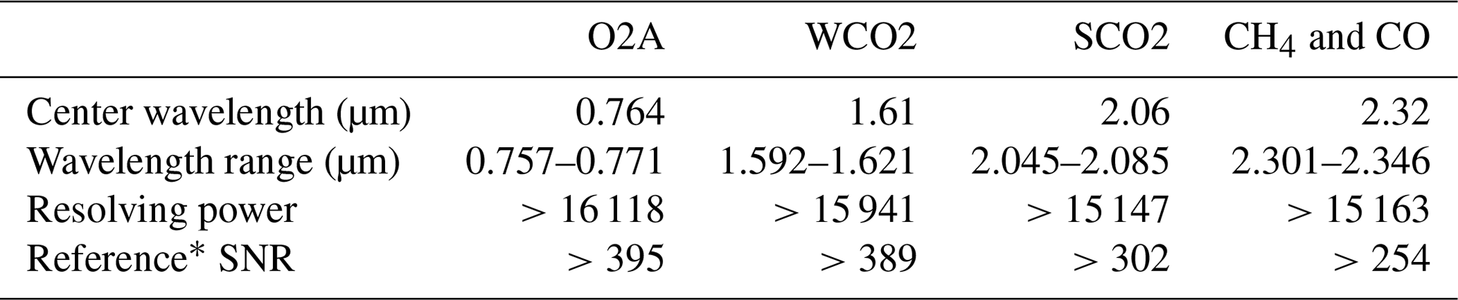
^* Reference SNR refers to the signal-to-noise ratio for the representative conditions at Railroad Valley, Nevada, at local noon on the summer solstice.

2.2 Scene inhomogeneity and slit homogenizers

Following Caron et al. (2019), the ISRF is defined by

$$\begin{array}{}\text{(1)}& \begin{array}{rl}\mathrm{ISRF}(\mathit{\lambda }-{\mathit{\lambda }}_o)& =\left[S\left({\displaystyle \frac{x}{M}}\right)\cdot {\mathrm{PSF}}_{\mathrm{spec}}\left(x\right)\cdot {\mathrm{PSF}}_{\det }\left(x\right)\right]\\ & \cdot \mathit{\delta }\left(x-{\displaystyle \frac{\mathit{\lambda }-{\mathit{\lambda }}_o}{k}}\right),\end{array}\end{array}$$

where

• S is the scene illumination, and M is the spectrometer magnification factor that maps the slit width dimension to the image on the detector;

• PSF_spec and PSF_det represent the 1-D optical response (including aberrations and diffraction) of the spectrometer and the response of the detector pixel (treated as a boxcar function), respectively, after averaging the corresponding 2-D function in the along-slit direction; and

• δ represents the change in variable from the detector position x (where x=0 is the center of the detector) to the wavelength grid centered at wavelength λ_o, assuming spectral dispersion k.

In trace gas retrievals, high-resolution radiance spectra are convolved with the assumed ISRF, typically measured during pre-flight instrument characterization (e.g., Lee et al., 2017), prior to comparison with observed radiances. Any mischaracterization of the ISRF can thus lead to errors in retrieved trace gases. One such mischaracterization occurs when brightness varies across width of the slit field of view (FOV) so that the function S is not constant. In this case, the ISRF is distorted relative to the ISRF measured pre-flight. These brightness variations can be due to gradients in surface albedo caused by different land surface types within the scene as well as partial cloud cover. In Landgraf et al. (2016) and Hu et al. (2016), these sorts of variations were shown to lead to significant errors in XCH₄ and XCO using simulations. Figure 1 shows one example of MODIS-observed albedo variations in three GeoCarb-relevant bands and the resultant impact on the normalized ISRF at the center wavelength in each of the four GeoCarb bands. The left panel shows the variation in 500 m MODIS black-sky albedo within a single GeoCarb footprint for the three MODIS bands nearest the GeoCarb spectral bands: Band 2 (0.85 µm), Band 6 (1.64 µm), and Band 7 (2.1 µm). The right panel shows the effect of a strong transition from brighter illumination to darker illumination: the resultant functions (ISRF_S's) are skewed to the left relative to the uniform illumination-derived functions (ISRF_U's).

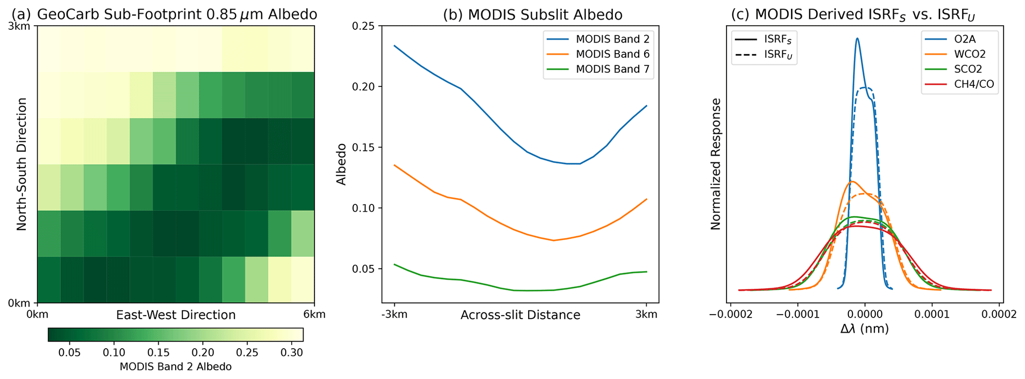
Figure 1 Variation in MODIS Band 2 (0.85 µm)-observed 500 m black-sky albedo for a single GeoCarb footprint (a); Band 2, Band 2 (1.64 µm), and Band 7 (2.1 µm) albedos averaged in the N–S direction (b); and the resultant normalized ISRFs for the center wavelength in each of the four GeoCarb bands in Table 1 (c). ISRF_S denotes the ISRF computed from (Eq. 1) with the illumination profile in the center panel, while ISRF_U uses a flat illumination profile. In this figure, the Band 7 albedo was used for the CH₄–CO band for simplicity. MODIS data demonstrate variation for a representative GeoCarb footprint near the southern Great Plains (SGP) research facility near Lamont, Oklahoma, on 18 June 2014.

One-dimensional SHs have been discussed previously (Sierk et al., 2017; Bauer et al., 2017; Caron et al., 2019) as a method of reducing the influence of brightness variations on the ISRF. Successful reduction in inhomogeneities was demonstrated at the breadboard level (Sierk et al., 2017). Based on the experimental and theoretical results in these previous studies, prototype 36 µm wide 1-D SH devices were procured from two vendors with depths of approximately 0.5, 1.0, and 1.5 mm, yielding six total devices. Each SH device consists of a thick slit made with two parallel mirrors, as is depicted in Fig. 2. The distance between the two mirrors is equivalent to the slit width. The two mirrors will create multiple reflections that homogenize the radiance at SH input. After a certain distance equal to the SH depth the illumination reaches the SH output and is homogenized. It is then delivered to the spectrometer. The performance testing of these devices and the theoretical interpretation of the results are the subject of this work.

Figure 2 The slit homogenizer is composed of two parallel mirrors separated by spacers. The slit opening is defined by its length (X dimension) and width (Y dimension) as for a regular slit. The slit homogenizing function comes from the third dimension (depth), where multiple reflections homogenize the illumination.

3 Slit homogenizer response modeling

3.1 Principles of slit homogenizer modeling

The simulated GeoCarb 1-D SHs are defined by two parameters: the slit width w and the slit homogenizer depth L, as depicted in Fig. 2. L is the extent of the reflective surfaces in the direction of light propagation and defines how many multiple reflections take place.

Modeling the SH response was discussed in detail in other references (Caron et al., 2019; Bauer et al., 2017), and so we summarize the main aspects here. The model computes the intensity distribution at the SH output for every possible position of a stimulus (source point or diffraction PSF) at the input plane using, for example, Eq. (3) in Bauer et al. (2017). The obtained intensity profiles are stored in a “transfer matrix” (Caron et al., 2019). The response of the SH to an arbitrary intensity distribution is then computed by proper weighting and addition of the relevant transfer matrix columns.

Let us assume that a point source is imaged on the SH entrance. When the SH entrance is observed from the SH output it appears to be illuminated with multiple point sources, which are aligned and placed at regular intervals: the original point source as well as all its mirror images after reflection on the two mirrors, as is shown in Fig. 3. To compute the intensity at the SH output one needs to add the contributions from the original point source plus all its mirror images, accounting for possible interferences due to their optical path difference.

This can be done in two ways:

• The interference model uses simple complex addition. The input stimuli are source points emitting light within a cone that corresponds to the system F number. This type of model is quite flexible and fast but gives only approximate results and might not exactly conserve energy (Caron et al., 2019).

• The diffraction model expresses the input stimuli as a diffraction point spread function (PSF) obtained with the optical system placed in front of the SH input plane, and a diffraction integral is used for propagation through the SH. This type of model is more accurate, but its computation time is significantly longer. For a rectangular pupil, thanks to the separability of the along-slit (X in Fig. 2) and across-slit (Y in Fig. 2) directions a 1-D diffraction model can be used, with an acceptable computing time. Modeling a circular pupil like GeoCarb's is more demanding and was not performed.

In the experiments that follow, we utilize the diffraction integral technique for maximum accuracy.

3.2 Specifications due to gold coating

In this work, existing SH models (Bauer et al., 2017) were upgraded to include the impacts of the properties of gold reflective coatings, particularly with regard to polarization, which were not included in the previous studies. These upgrades were undertaken in large part to explain the behavior observed in the measurements described later in the paper that seem to result from GeoCarb's narrow slit and relatively fast beam ($f/\mathrm{4.5}$). The gold optical constants were computed with a Lorentz–Drude model with parameters taken from Rakić et al. (1998). The phase of the mirror complex reflectance plays a crucial role in the SH response, so we now discuss it in detail. The definition of the phase shift that occurs at reflection depends on two aspects:

• The sign of the phase is changed depending on the complex notation that is used, with positive or negative complex exponentials e^+iωt or e^−iωt.

• If, at normal incidence, the vectors for incident and reflected electric fields are equal or differ by a minus sign, a 180^∘ phase shift can be induced in the reflectance phase.

Our equations to compute the gold reflectance are taken from Macleod (2017). A positive complex exponential e^+iωt is used, and the electric fields (incident and reflected) coincide at normal incidence for both S and P polarization. The computed phase shifts are displayed in Fig. 4.

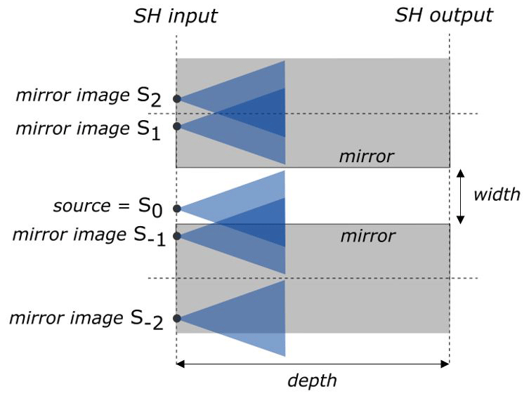
Figure 3 A point source S₀ is imaged at the SH input. The rays emitted by S₀ are reflected multiple times by the two mirrors, creating images of S₀ (noted S₁, S₂, ..., etc. and S_-1, S_-2, ..., etc.). The total illumination seen at the SH output is the superposition of the rays emitted by the original point source S₀ and all its mirror images.

Figure 4 Phase shift at reflection on a thick gold layer, computed from Rakić gold index parametrization (Rakić et al., 1998) with definitions of polarization axes from Macleod (2017). (a) P polarization (P-pol), (b) S polarization. The 180^∘ shift in P-pol discussed in Fig. 5 is not included.

In order to incorporate the complex reflectance in the SH model, as discussed in Caron et al. (2019) it is necessary to make a 180^∘ correction for the P-polarized phase. A simple example helps to explain the need for this additional phase shift. Consider reflection on a substrate made of an ideal metal (with infinite conductivity). In the convention of Macleod (2017), where the incident and reflected electric field coincide at normal incidence, the phase shifts obtained at reflection are equal to 180^∘ at all angles and for both polarizations. These 180^∘ dephasings are an intrinsic property of the ideal metal.

Figure 5 Definition of phase reflectance in P polarization. (a) Situation close to normal incidence. The P-polarized electric fields before and after reflection are defined according to McLeod (2017) and are pointing in the same direction. For an ideal metal with infinite conductivity the phase shift at reflection is 180^∘. (b) Situation close to grazing incidence. We adopt the opposite definition to McLeod (2017), with electric fields pointing in opposite direction if the incidence angle was reduced to zero. At grazing incidence it means the electric fields are pointing towards the same direction. For an ideal metal the phase shift at reflection is now 0^∘ due to the different definition.

When the angle of incidence is increased to large values, the angle between incident and reflected rays increases by 180^∘ with respect to the situation at normal incidence (Fig. 5). In this process, the P-polarized electric field has also rotated by 180^∘. The phase shift of 180^∘ between incident and reflected electric fields in P polarization pointing in the same direction at normal incidence becomes a phase shift of 180^∘ between two electric fields pointing now in the opposite direction at grazing incidence due to the beam rotation. This phase shift is equivalent to a 0^∘ phase shift for two electric fields that are pointing in the same direction at grazing incidence (Fig. 5, right). In the SH model, we assume that the direction of the electric fields does not change at reflection at grazing incidence. It is therefore necessary to add an extra phase offset of 180^∘ in P polarization. No such offset is required in S polarization.

3.3 Sizing of the GeoCarb SH prototypes

An earlier version of the SH simulator (without polarization dependence) detailed in Caron et al. (2019) was used to estimate the optimal depth of the homogenizer for all four GeoCarb bands, which share a single slit in the GeoCarb design. As is discussed above, the simulator generates a transfer matrix that depends on depth and wavelength.

If only pure geometric optics is considered and if the instrument has a rectangular pupil, it can be easily shown that after a propagation distance equal to multiples of 2F#w the beam uniformly illuminates the slit output. From the perspective of geometric optics, if the SH depth is equal to a multiple of 2F#w the slit homogenization is then perfect for a rectangular pupil. In reality this simple rule of thumb is not valid due to the presence of interferences.

To determine the optimum depth for the slit homogenizer for GeoCarb, we simulated polarization-independent transfer matrices for depths from 0.1 to 2 mm at all four wavelengths of interest (listed in Table 1) using the previously documented SH model (Bauer et al., 2017). We then randomly generated an ensemble of input scenes with inhomogeneities that had an average coefficient of variation in scene brightness of 20 % on size scales of about $\mathrm{1}/\mathrm{5}$th of a slit width. We applied the computed transfer matrix for each depth to the ensemble, and the resultant coefficient of variation in the output was calculated. The median reduction in coefficient of variation for each wavelength at each slit depth was used as the metric for selection.

After an initial ramp-up in performance at the lowest depths, the reduction factors were relatively independent of the homogenizer depth; however, there were conspicuous dips in performance at specific depths that were not coincident for all four wavelengths. These dips are due to some periodicity in the interference patterns as the light propagates along the depth of the slit. GeoCarb uses a single 36 µm wide slit, so we chose to investigate three depths that optimized performance across all four bands simultaneously, which were approximately 0.5, 1, and 1.5 mm.

4 Experimental characterization

In order to assess the performance of the six different SH prototypes, a breadboard test setup was constructed at the Institut für Technische Optik (ITO). This section details the optical design and fabrication employed in the testing.

4.1 Measurement setup

The homogenization performance was evaluated based on recordings of the near-field intensity distribution at the exit of each SH, while the input was illuminated with different illumination patterns (realized by a knife edge). All measurements were performed at four different wavelengths (0.76, 1.62, 2.05, and 2.33 µm) and for polarizations parallel as well as orthogonal to the slit. Additionally, the throughput efficiency was measured.

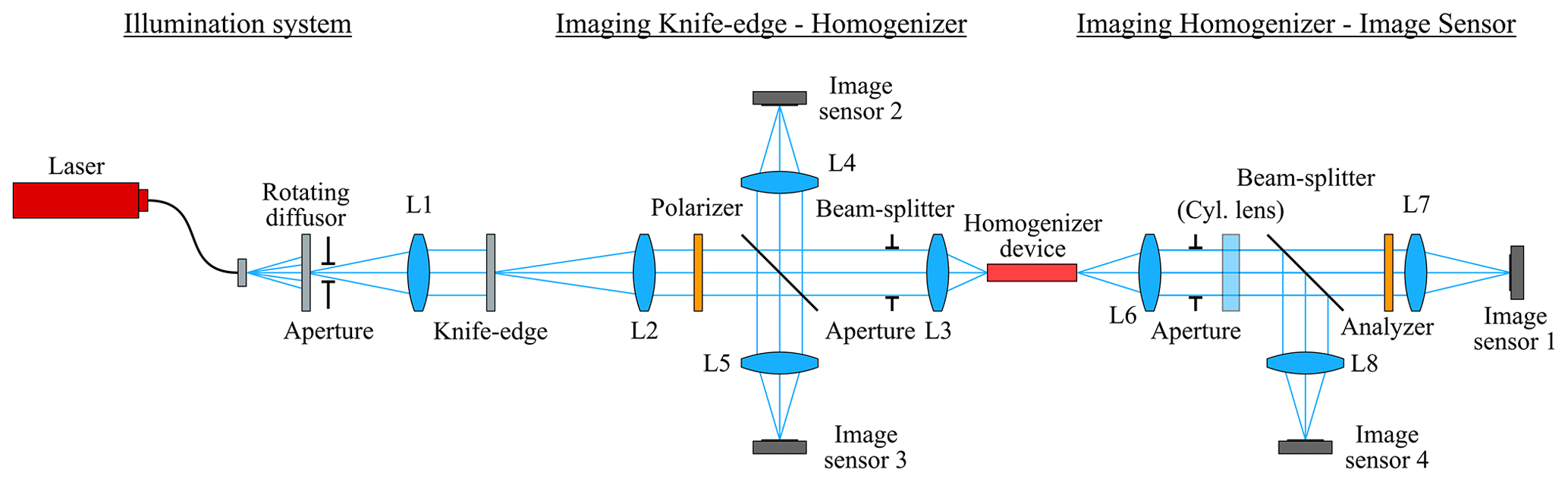
Figure 6 depicts the setup used for the measurements. To achieve spatially incoherent light we employed a diffuser approach based on the combination of a fixed and a rotating diffuser (ground glass, 220 grit from Edmund Optics). Fourier geometry (L1 in Fig. 6, f₁=100 mm, image-sided telecentric) is used to homogenize the light in the plane of the knife edge and to make sure that every point in this plane receives the same angular light distribution (telecentric illumination).

The following mono-mode fiber-coupled monochromatic sources have been employed:

• 0.76 µm – tunable laser from Sacher Lasertechnik Group, model TEC 500, serial no. P-770-0517-01003;

• 1.62 µm – tunable laser from Sacher Lasertechnik Group, model TEC 500, serial no. P-1650-0615-00941;

• 2.05 µm – YE3085 single-mode fiber pigtailed diode laser from NASA Jet Propulsion Laboratory at approximately 3 mW;

• 2.33 µm – EP2327-0-DM-TP39-01 from Eblana Photonics at approximately 2.6 mW.

The knife edge (Edmund optics no. 36-137) with variable orientation (micromechanical adjustable mount) serves to obscure part of the slit and thus to introduce a sharp cutoff in illumination across the homogenizer, simulating an extreme version of the typical image taken from space by the GeoCarb instrument.

The knife edge is imaged by a double-sided telecentric system at an F number of 4.5 into the entrance plane of the SH. For 0.76 and 1.62 µm we used two achromatic lenses (Thorlabs AC254-150-B, focal length f₂=150 mm, and Thorlabs AC050-010-B-ML, focal length f₃=10 mm). The paraxial magnification is $-\mathrm{0},\mathrm{067}$. For 2.05 and 2.33 µm we used an air-spaced achromat (Thorlabs ACA254-200-D, focal length f₂=200 mm) and a plano-convex spherical lens (Thorlabs LA0309-E, focal length f₃=15 mm). The paraxial magnification is −0.074. Both systems were optimized in Zemax to minimize the rms spot radius under the requirement to maintain telecentricity.

Figure 6 Setup for the near-field measurements.

Coherence reduction and homogeneity were verified by measurement of the speckle contrast in the plane of the SH. To validate the image quality and homogeneity at 0.76 µm, we placed an image sensor (XIMEA MQ042RG-CM) without cover glass at the entrance plane of the homogenizer (see Fig. 7). The line cut along the image of the knife edge shows a standard deviation of 1 % after subtracting the linear contribution. We took the contrast $(I_{\max }-I_{\min })/(I_{\max }+I_{\min })$ as a measure of homogeneity. For 2.05 and 2.33 µm this results in 0.36 % and 0.40 % (after applying a Gaussian filter with σ=15 pixels to reduce shot and read noise arising from the light sources and image sensors).

Figure 7 (a) Image of the pick-off mirror in the position of the device input, taken by image sensor without cover glass. (b) Intensity along the horizontal line depicted in (a).

The slit homogenizer can be moved in all three dimensions using high-precision piezo stages (Physik Instrumente PI Q-545.240 linear stage, PI E-873.3QTU controller, repeatability error of 200 nm). The orientation of the SH mount is parallel to the optical axis to better than ±0.1^∘ (aligned using two additional helium–neon alignment lasers).

The intensity distribution at the exit of the SH is imaged by a double-sided telecentric system (L6 and L7 in Fig. 6) onto the image sensor with an F number of 4.0.

For the measurements at λ=0.76 and 1.62 µm L6 and L7 are achromatic lenses with focal lengths of f₆=10 mm and f₇=200 mm (Thorlabs AC050-010-B-ML, AC254-200-B-ML). The simulated paraxial magnification of this system is −20 parallel to the slit and −25.9 orthogonal to the slit, respectively.

In order to be able to judge homogenization performance and to see possible crosstalk it is preferable to use anamorphotic imaging so that vertical structures in the output plane of the device are resolved, while still the lateral position along the slit on the input side is maintained on the image sensor side. To this end we used an additional cylindrical lens (λ=0.76 µm: LK1336RM-B; λ=1.62 µm: LK1336RM-C) while imaging the exit of the device onto the image sensor.

For λ=2.05 and λ=2.33 µm, it was not possible to achieve a near-diffraction-limited anamorphotic setup with stock lenses. Instead, a rotationally symmetric system was used. This way only the device output plane was imaged sharply onto the image sensor, but the measurements at λ=0.76 and λ=1.62 µm suggested that this does not result in a loss of information. L6 and L7 are changed to LA0309-E (focal length f₆=15 mm) and ACA254-300-D (focal length f₇=300 mm). The (simulated) paraxial magnification of the system is −31.8 (2.05 µm) and −32.7 (2.33 µm).

The polarizer (λ=0.76 µm: Thorlabs LPNIRE100-B; λ=1.62 µm: LPIREA100-C; λ=2.05 µm and λ=2.33 µm: LPNIRA050-MP2) is placed between L2 and L3 as well as a second analyzer device just prior to L7, together with a half-wave plate to rotate the polarization from the laser output.

In the NIR, a scientific CMOS image sensor (PCO edge 3.1 2048×2048 pixels, 6.5 µm pixel pitch) was used. At λ=1.62 µm a Raptor Photonic InGaAs image sensor (Ninox 640 VIS–SWIR, 640×512 pixels, 15 µm pixel pitch) was used, and at longer wavelengths a Xenics image sensor (Xeva-2.35-320-TE4, 320×256 pixels, 30 µm pixel pitch) was used.

The beam splitters and image sensors 2, 3, and 4 were only used for alignment and were removed while taking the measurements.

4.2 Reduction in interference effects

Some interference effects were caused by the cover glass of the main image sensor. For λ=0.77 µm (PCO edge 3.1) this can be avoided by slightly tilting the sensor until the spatial frequency of the fringes is sufficiently large to be ignored.

For the other wavelengths and image sensors this method does not work, but since the interference fringes are spatially constant, we eliminated the fringes by averaging of spatially shifted images. The image sensor is mounted on a vertically movable stage (Thorlabs MLJ050). Images are taken for different heights of the sensor with a displacement of multiples of the pixel pitch. The image of the slit moves over the sensor area and thus appears at different positions compared to the interference pattern for each image. Image processing is then used to digitally shift the captured image back considering the difference in the sensor height. This is possible since the accuracy of the stage is high compared to the pixel pitch. Averaging of the shifted images results in a significant reduction in the interference effect.

4.3 Measurement procedure

Measurements were performed for the six devices mentioned previously (two vendors supplied devices with depths of 0.5, 1.0, and 1.5 mm) for different input and output polarizer settings (S/P) for different positions of the device with respect to the input knife edge illumination (in steps of 2.5 µm). For each setting 20 images were recorded: 10 for the illuminated device and 10 without illumination as a “dark reference” (to be subtracted during image processing). Figure 8 shows a typical result for four different measurements (only regions near the slit image are shown) and the normalized intensity cross section along the vertical.

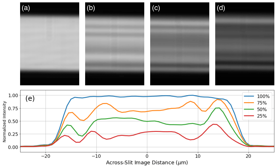
Figure 8 (a, b, c, d) Typical raw images recorded on the image sensor as the knife edge obscures more and more of the incoming beam (only regions of interest shown): (a) fully illuminated (100 %) (b) 75 % unobstructed, (c) 50 % unobstructed, and (d) 25 % unobstructed. (e) One-dimensional profiles obtained by averaging the panels in the top row along vertical cross sections in the top image, which would correspond to variations across the shorter dimension of the slit. Note the decreasing intensity as the knife edge obscures more of the light, apparent in the change in brightness of the figures from left to right. Note also that the slit homogenizer effectively reduces the sharp gradient that would be present along a knife edge with a typical slit and spreads the light fairly uniformly across the image.

4.4 Modification for throughput measurement

The throughput was measured with a slightly modified configuration for simplicity. The pick-off mirror was replaced by a circular aperture to illuminate only a defined area. Images were taken under parallel and orthogonal input polarization. Reference images were taken with thin slits (Edmund no. 58-541 and no. 58-542) of known width (measured using a confocal microscope), as well as without an air slit or slit homogenizer to account for potential laser intensity fluctuations. The slit homogenizer throughput values are treated as relative to the air slit measurements as the design trade for GeoCarb is between these two options.

5 Results

The performance test results and model simulations are presented in this section, as well as some further investigations with the model to explain some of the unexpected findings uncovered during testing.

5.1 One-dimensional SH measurements

The measurements were taken as described in the previous sections for different positions of the knife edge, and the resulting 2-D images were averaged to produce the 1-D profile of the homogenized slit images. We compare the results for fully illuminated and 50 % illuminated test data, as well as the throughput performance, below.

5.1.1 Homogenization performance

As described above, 2-D images were taken for each SH as it was moved across the knife edge, gradually obscuring larger and larger portions of the SH. The efficacy of the SH is judged by how well it reproduces the normalized profile of illumination of the fully illuminated SH when the input illumination is partially obscured by the knife edge after averaging in the across-slit direction. Importantly, the image of a fully illuminated SH is not the same as that of a typical air slit due to the interference effects. However, these effects are measured and would be taken into account during the pre-flight ISRF characterization (e.g., Lee et al., 2017) for GeoCarb and so are not cause for concern. Thus, the homogenization performance for each device is compared against the image of the fully illuminated SH for that device only.

Figure 9 Across-slit illumination as a function of slit position for horizontally (left column) and vertically (right column) polarized light. The colors represent the different devices (D1–D6) detailed in Table 2. Solid lines depict fully illuminated scenes, normalized to the maximum value, while dashed lines represent the illumination pattern resulting from 50 % of the illumination being blocked by a knife edge (normalized by the maximum value of the corresponding fully illuminated slit image), which is apparent from the lower signal in the dashed lines.

Figure 9 shows the results of the measurements for each of the six devices at the four wavelengths of interest, when the slit is fully illuminated and partially illuminated, for H (left column) and V (right column) polarizations. The 50 % illumination results are not normalized in order to show the effects of the reduction in throughput due to partial obscuration of the slit entrance. A few observations are noteworthy. All of the devices reduce the nonuniformity that would be apparent in the 50 % illuminated images in the presence of an air slit only, which is apparent from the somewhat more even distribution of light across the width of the slit image. Interference effects due to the multibeam interferences that take place manifest as oscillations in the 1-D profiles. These effects become stronger the less of the entrance slit is illuminated and weaker as the wavelength grows. We found, somewhat unexpectedly, that the SH devices prefer one polarization (H) over the other (V). This is most apparent as a drop in throughput for V relative to H as seen in Table 2. We note that this effect generally gets more pronounced as the depth of the homogenizer grows. The effect also gets more pronounced at longer wavelengths as opposed to shorter wavelengths.

5.1.2 Relative throughput measurements

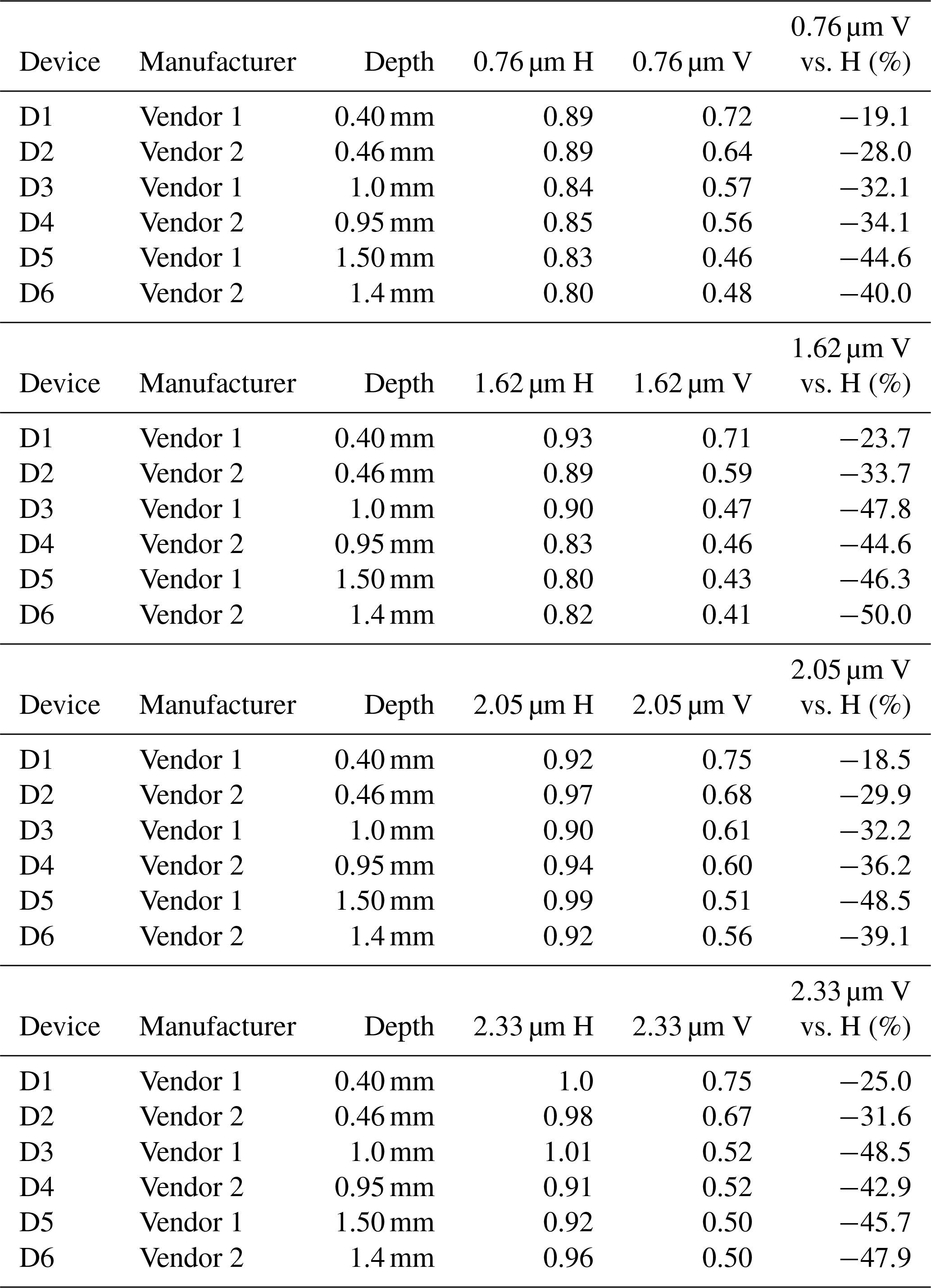
The relative throughput measurements show a strong reduction for vertically polarized light, especially at increased device depth (see Table 2). The results show a dependence on vendor, wavelength, and slit homogenizer depth. The narrowing in the V polarization relative to the H polarization increases with depth as well as wavelength (with the exception of the 1.5 mm device by Vendor 1). These variations imply a preference for incoming light with H polarization, which could complicate interpretation of radiances taken from space where the polarization state in incident light will be unknown. The GeoCarb instrument does not include mitigation for polarization of incoming light, such as a linear polarizer or polarization scrambler.

Table 2 Throughput as compared to a thin slit for different devices with an F number of $f/\mathrm{4.5}$ for horizontal (H) and vertical (V) polarization.

5.2 Comparison of SH models with Zemax

In order to explain the polarization-dependent features in the SH measurement data, we employ the diffraction SH model. To validate our model, a comparison with simulations using the Zemax software package was performed. A 1-D SH was entered in Zemax non-sequential mode. Two parallel mirrors were defined, coated with gold (using the Rakić parameterization from Rakić et al., 1998), with a length of 36 µm and with a length of 1.0 mm. A small source was defined, emitting coherent light at a wavelength of 1600 nm in a cone with 0^∘ angle in the along-slit direction and an F number of 4.5 in the across-slit direction.

More elaborate models could be set up in Zemax with a source emitting a 2-D cone of light, but this would require a more complicated design to create an astigmatic beam, which was not done in this work. Monte Carlo simulations were used with 10⁶ to 10⁷ rays. Execution time was typically between 1 and 20 min depending on the required sampling and targeted accuracy (both impacting the required number of rays).

The SH analytical model assumes a scalar wave in the sense that optical path differences and phase shifts are calculated for each ray and combined directly to compute the intensity where the rays interfere. By contrast, Zemax propagates the real electric field along the ray and computes interferences with real electric field vectors: interferences are computed separately for the X, Y, and Z components, and intensities are added at the end.

We found a reasonable qualitative agreement between the Zemax and analytical model results. In Fig. 10 we present the obtained intensity profiles at slit output as well as the ISRFs. The ISRFs are computed by convolving the intensity profiles with a Gaussian PSF of the full width at half maximum (FWHM) equal to $\mathrm{1}/\mathrm{6}$ of the SH width, which represents the optical point spread function of the imaging optics of the experimental setup described in the previous sections. Both models assume a SH width w=36 µm, depth L=1 mm, F number = 4.5, and λ = 1.6 µm. Though this agreement would not be sufficient to use the analytical model results in place of the Zemax (or real) ISRFs, it is sufficient to understand the mechanism underlying the polarization dependence of the ISRF features, discussed in the next section.

5.3 Polarization-dependent ISRF width

We investigated the cause of the polarization dependence in the simulated and measured ISRFs using the interference SH model. This effect was linked to the different phase shifts gained by the electric field at the reflection on the gold layer. When both dephasings are artificially set to the same value in the model, simulations show nearly identical transfer functions in P and S polarization and nearly no variation in the ISRF width, which implies that the difference in reflectance amplitude with polarization plays almost no role.

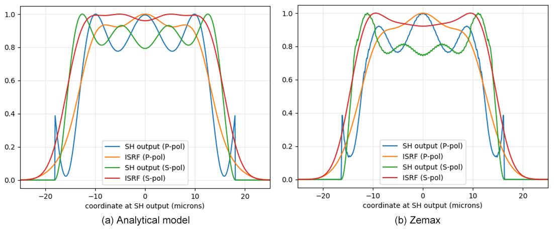
Figure 10 SH output illumination and resulting ISRF in P and S polarization for a SH length of 1 mm, F number = 4.5, and λ=1600 nm. (a) Analytical model, (b) Zemax. A square pupil and an interference model were used.

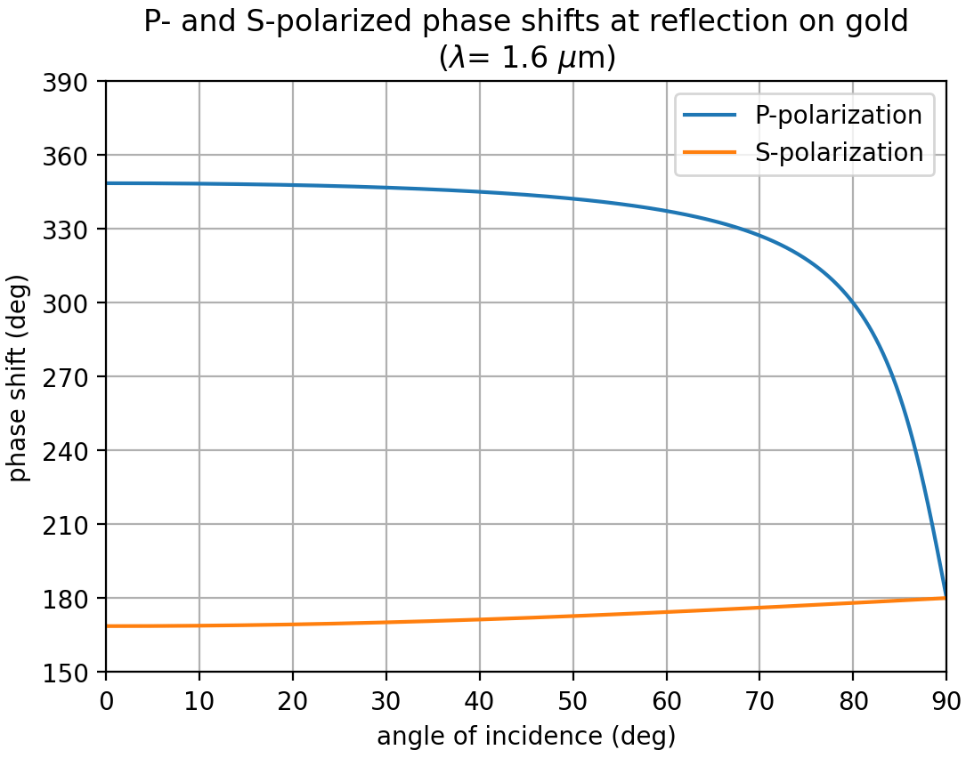
Figure 11 P-polarized and S-polarized phase shifts at reflection on gold as a function of the angle of incidence, for λ=1.6 µm. The 180^∘ phase shift specific to P-pol shown in Fig. 5 is included.

To understand the role of the phase shift, it is necessary to look at its variations with angle of incidence. In Fig. 11, we represent the phase shifts in both polarizations, including the 180^∘ phase offset specific to grazing incidence in P polarization. When the angle of incidence is very large, or equivalently when the SH is operated with a beam with large F number, then both phase shifts are close to 180^∘, and there is almost no polarization effect. When the angles of incidence are decreased (i.e., going to lower F numbers) the phase shifts start to differ. In particular, the phase shift in P polarization starts to become large and easily reaches 270^∘ (so a difference of 90^∘). Then a clear polarization effect occurs.

This applies for the relatively low F number of GeoCarb. Additionally, as can be seen on the plots showing the output illumination and the ISRFs, the magnitude of the ISRF width variation is comparable to one oscillation period in the interference pattern. This suggests that the relative change in ISRF width will be smaller for a slit that is significantly wider than the size of one diffraction pattern (Airy disk). For this reason, the polarization effect becomes clearly visible due to GeoCarb's narrow slit (36 µm) and becomes more pronounced at larger wavelengths.

5.4 Predicted transmittance

Next, the SH transmittance was investigated. The amount of intensity transmitted by the SH when its input is illuminated with a uniform intensity profile was computed using a diffraction model. Diffraction models are not only more accurate than interference models; they also rigorously conserve energy thanks to the properties of diffraction integrals, so they are well suited for transmittance calculations. The SH transmittance was obtained with a summation of the transfer matrix along one dimension, which corresponds to the case where the SH input is fully and uniformly illuminated.

The results are presented in Fig. 12. Three cases are studied.

• Ts–Tp radiometry only. As a reference, we made a simple SH transmittance calculation with a modified interference model, where all effects from the interference were suppressed. This model gives the net effect of the finite reflectivity of the gold coating, combined with the angles of propagation inside the SH.

• Ts–Tp diffraction model phase = 180^∘. The transmittance was computed with the diffraction model, assuming that the phase shift at reflection keeps the ideal value of 180^∘ for all angles of incidence.

• Ts–Tp diffraction model gold. Finally the transmittance was computed with the diffraction model and a real gold layer.

We immediately see that the three models predict a nearly identical transmittance in S polarization that is close to 100 %, while they give very different losses in P polarization. Taking the simulation without interferences (first curve) as a reference, we notice that including diffraction effects with a 180^∘ phase shift results in a slight increase in the losses. This increase can be easily explained by the fact that diffraction sends some light at larger angles than what geometric optics predicts, creating stronger losses. By contrast, the diffraction model with gold dephasings predicts an even stronger increase in losses. This increase is surprising as it is purely due to the phase shifts at reflection (the amplitude of reflection coefficients being unchanged). One possible explanation is that the gold phase shift in P polarization has a strong influence on the diffracted angles so that part of the incident light experiences many more reflections inside the SH and a much higher absorption. The model results are not totally in sync with the obtained experimental results shown in Table 2, though the model does predict larger relative transmittance in the shortest wavelength versus the longest wavelength. Given the variation in results from the two vendors, it is clear that the manufacturing process yields devices with some degree of variability.

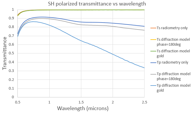
Figure 12 SH transmittance vs. polarization and wavelength for w=36 µm, L=1 mm, and F number = 4.5. We note the transmittance for S-polarized light is nearly identical for the three different models, while the P polarization response depends significantly on the treatment of the phase shift interaction with the surface. The transmittance drops precipitously when we allow the phase shift to vary at reflection in response to a realistic gold surface.

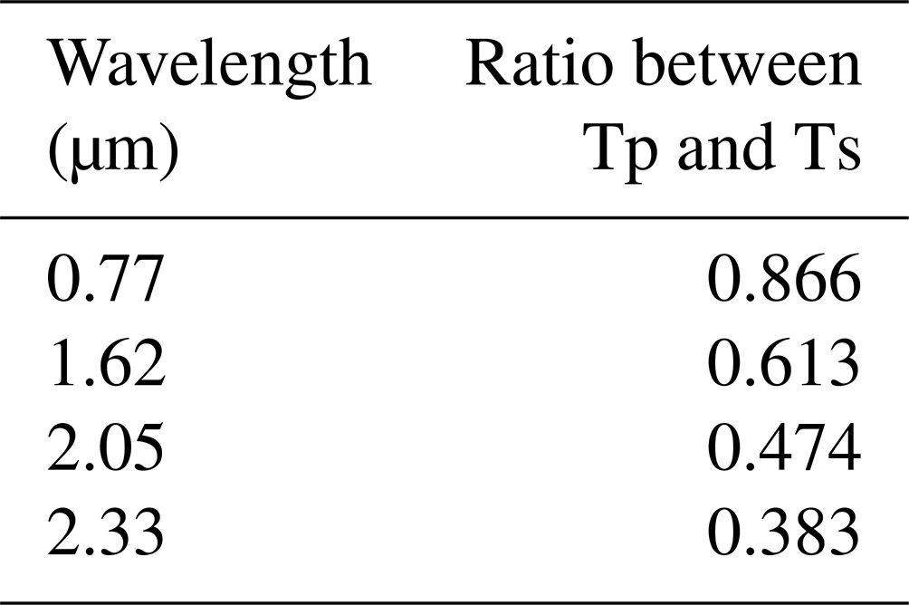
Table 3 Ratio between P-polarized and S-polarized transmittances predicted for GeoCarb (w=36 µm, L=1 mm), using a SH diffraction model and assuming a rectangular pupil (F number = 4.5).

6 Discussion

The measurements and modeling together provide a strong argument that performance of 1-D slit homogenizers of the type considered for GeoCarb (i.e.,  plane-parallel, gold-coated mirrors) is highly sensitive to the polarization of incoming light. The polarization response of the instrument itself, including important components such as the grating, can be characterized in pre-flight calibration, but the polarization state of the incident reflected sunlight is itself unknown and is a function of particles in the atmosphere that scatter light as well as the surface properties. This could lead to significant errors in trace gas retrievals using spectra through the difficulty in disambiguation of albedo and polarization states. For example, two scenes with identical trace gas column mole fractions but different polarization states would be hard to distinguish from scenes with identical polarization states but different trace gas amounts, even if the instrument were perfectly characterized. Another important challenge is the implication that the ISRF will be strongly polarization-dependent and thus change from scene to scene in a similar way as it would with no slit homogenizer present due to the scene brightness variations. Further, there is the potential of using other space-based sensors to try to get a handle on surface brightness, but no such information exists for polarization. Finally, the signal-to-noise ratio will also be highly dependent on polarization, and the lower efficiency of the SH would almost certainly lead to poorer-quality retrievals. In a very real sense, the 1-D devices add complexity to the instrument design but do not reduce uncertainty. For this reason, the slit homogenizer was removed from the GeoCarb design.

The upcoming Sentinel-5 mission includes a 1-D slit homogenizer in their design, as is discussed in Köhler et al. (2021) and Hummel et al. (2021). These results support the Sentinel-5 instrument design (1) because the instrument includes a polarization scrambler and (2) because their slit is 120 µm or 3–4 times wider than GeoCarb, their F number is close to 10 (which is a very different optical regime than the GeoCarb instrument), and their SH was chosen with all of these considerations in mind. Future missions that choose to include a slit homogenizer would do well to perform an optical performance analysis of their slit assembly prior to installation and definitely include an optical element that removes polarization on the incoming light.

7 Conclusions

We have presented both experimental and simulated results related to the performance of 1-D SH devices consistent with the GeoCarb optical design. We found that the devices exhibited a strong sensitivity to the polarization of the light incident on the slit. This was apparent in both the width of the slit image and the relative throughput of the different devices. The difference between the two orthogonal polarization states grew worse as wavelengths got longer. We then augmented a model of the slit homogenizer to demonstrate that this narrowing is caused by the reflection on the gold coatings on the mirrors that lead to a phase shift between the P and S polarizations. It seems likely that different materials could be used with better results, but the space application required for GeoCarb limited our interest in that investigation.

Future work involves the implementation of these measurement results in a retrieval framework similar to that described in O'Brien et al. (2016) to better understand the tradeoff between the albedo effects and the polarization sensitivities in the two designs.