the Creative Commons Attribution 4.0 License.
the Creative Commons Attribution 4.0 License.
 | 17 Apr 2023
Further validation of the estimates of the downwelling solar radiation at ground level in cloud-free conditions provided by the McClear service: the case of Sub-Saharan Africa and the Maldives Archipelago
William Wandji Nyamsi
Yves-Marie Saint-Drenan
Antti Arola
Lucien Wald
Being part of the Copernicus Atmosphere Monitoring Service (CAMS), the McClear service provides estimates of the downwelling shortwave irradiance and its direct and diffuse components received at ground level in cloud-free conditions, with inputs on ozone, water vapor and aerosol properties from CAMS. McClear estimates have been validated over several parts of the world by various authors. This article makes a step forward by comparing McClear estimates to measurements performed at 44 ground-based stations located in Sub-Saharan Africa and the Maldives Archipelago in the Indian Ocean. The global irradiance received on a horizontal surface (G) and its direct component received at normal incidence (BN) provided by the McClear-v3 service were compared to 1 min measurements made in cloud-free conditions at the stations. The correlation coefficient is greater than 0.96 for G, whereas it is greater than 0.70 at all stations but five for BN. The mean of G is accurately estimated at stations located in arid climates (BSh, BWh, BSk, BWk) and temperate climates without a dry season and a hot or warm summer (Cfa, Cfb) or with a dry and hot summer (Csa) with a relative bias in the range [−1.5, 1.5] % with respect to the means of the measurements at each station. It is underestimated in tropical climates of monsoon type (Am) and overestimated in tropical climates of savannah type (Aw) and temperate climates with a dry winter and hot (Cwa) or warm (Cwb) summer. The McClear service tends to overestimate the mean of BN. The standard deviation of errors for G ranges between 13 W m−2 (1.3 %) and 31 W m−2 (3.7 %) and that for BN ranges between 31 W m−2 (3.0 %), and 70 W m−2 (7.9 %). Both offer small variations in time and space. A review of previous works reveals no significant difference between their results and ours. This work establishes a general overview of the performances of the McClear service.
- Article
(4154 KB) - Full-text XML
-
Supplement
(23024 KB) - BibTeX
- EndNote


Solar radiation received at the ground is the main driver behind the weather and climate systems on the planet. It is one of the essential variables in climate (Bojinski et al., 2014; Lean and Rind, 1998), air quality (GEO, 2010), the terrestrial and marine environment (Dantas de Paula et al., 2020; GEO, 2014), and renewable energies (Ranchin et al., 2020). Furthermore, it has an impact on human health (Juzeniene et al., 2011) and many other aspects of our daily lives and our activities as shown by the many examples given in Lefèvre et al. (2014) and Wald (2021). The density of power received from the sun on a horizontal surface at ground level and integrated over the shortwave portion of the electromagnetic spectrum is called the surface solar irradiance here, abbreviated as SSI. Other terms may be found in the literature, such as solar flux, downwelling solar irradiance at the surface, downwelling shortwave flux, or surface incoming shortwave irradiance. The SSI is the sum of its direct and diffuse components. Roughly speaking, the radiation measured on a horizontal surface looking in the direction of the sun is the direct component, denoted B, while the diffuse component, denoted D, is the sum of the fluxes coming from the other directions of the sky and impinging on this surface. When it is necessary to clearly distinguish the SSI from its components, the SSI is called global SSI, often denoted G, with . Researchers in solar energy often term the SSI global horizontal irradiance, where horizontal means horizontal surface, abbreviated as GHI (see, e.g., Sengupta et al., 2021).
Of particular interest here is the SSI received in cloud-free conditions and often termed clear-sky SSI. It depends on the date and time of the day and geographic coordinates. It also depends on the concentrations of gases, though it is generally sufficient in the case of total radiation to consider the ozone and water vapor contents only, which are very variable, and to prescribe the concentrations of the other gases to standard values. As absorption depends on local conditions of temperature, density, and pressure, the vertical profile of these variables, as well as that of the volume mixing ratio of absorbing gases excluding ozone and water vapor, must be known. This profile also allows the calculation of the scattering effects of air molecules. The clear-sky SSI also depends on the optical properties of aerosols, which are highly variable in space and time. Usually, classes of aerosols are used, for example, sea salt or soot, which have been assigned average optical properties. The aerosol load is given by an aerosol optical depth known at one or more wavelengths, for example, 550 and 1240 nm, or else the optical depth at a given wavelength and Ångström exponent. Finally, the clear-sky SSI depends on the elevation of the ground above the mean sea level and on the reflective properties of the ground. Oumbe et al. (2014) found that G in cloudy conditions may be accurately approximated by the product of the clear-sky G by a cloud modification factor, also known as the clear-sky index, which does not depend on the properties of the cloud-free atmosphere. The error made in using this approximation is similar to the typical uncertainty associated with the most accurate pyranometers, except in the case of ground albedo greater than 0.7 for which the error is greater. This result underlines the importance of accurate calculation of the clear-sky SSI. A model estimating the clear-sky SSI is called a clear-sky model. It provides realistic upper limits of the SSI and contributes to quantifying the radiative effects of the clouds.
There are many clear-sky models described in the scientific literature (see, e.g., Gueymard, 2012; Sengupta et al., 2021; Sun et al., 2019, 2021; Yang, 2020). The McClear model is one of them. It has been developed under the auspices of the European Commission to support the Copernicus Atmosphere Monitoring Service (CAMS) delivering solar radiation at the ground in all sky conditions (Qu et al., 2017; Schroedter-Homscheidt, 2019). The original McClear model described in Lefèvre et al. (2013) was set into operation in 2012. After slight changes in 2013 (version v2), the current version, v3, was introduced in 2018 (Gschwind et al., 2019). Though it can be used as a stand-alone model, McClear is mostly being used in synergy with the 3 h estimates of aerosol properties and daily total column contents of water vapor and ozone provided by CAMS as inputs. The McClear service is the combination of McClear and CAMS (Schroedter-Homscheidt, 2019). It delivers time series of G and its direct and diffuse components at any site in the world and for any period from 2004 to date with a 2 d delay for the summarizations of 1 min, 15 min, 1 h, 1 d, and 1 month.
The McClear service has thousands of users, including academics, researchers, consultants, and companies in various domains (Gschwind et al., 2019). Its outputs are regularly confronted with ground-based measurements of irradiance made by pyranometers and pyrheliometers by either the team in charge of its development or by these users who provide valuable direct and indirect validations of the McClear service and feedbacks on its limitations. Such validations provide valuable information on the uncertainties of the outputs of the McClear service to non-expert users and indirectly give information on the aerosol properties given by CAMS in areas not covered by stations measuring aerosols properties such as the AErosol RObotic NETwork (AERONET). Several validations have been reported in the scientific literature dealing with many stations in various climates, but the cases of Sub-Saharan Africa and the western Indian Ocean have so far hardly been addressed. Gschwind et al. (2019) and Lefèvre et al. (2013) performed comparisons at stations located over the whole world except these regions. Sun et al. (2019, 2021) also dealt with the whole world and included measurements from the Southern African Universities Radiometric (SAURAN) in southern Africa. Yang (2020) dealt with stations in North America; Ceamanos et al. (2014) and Ineichen (2016) used stations in Europe, Israel, and Algeria, with Ineichen using one station at Mount Kenya (Kenya) and another one at Skukuza (South Africa). Other authors dealt with more local networks. Antonanzas-Torres et al. (2019) used two European stations, while Lefèvre and Wald (2016) and Eissa et al. (2015a, b) analyzed the consistency of the performances of McClear between several close stations in Israel, United Arab Emirates, and Egypt, respectively. Cros et al. (2013) studied the case of La Réunion, Corsica, and French Guiana. Dev et al. (2017) performed a comparison in Singapore, while Zhong and Kleissl (2015) performed their own in California. Chen et al. (2020) studied the case of the megacity Shanghai, and Alani et al. (2019) focused on Morocco. Mabasa et al. (2021) assessed the quality of McClear using 13 stations of the South African Weather Services in South Africa.
The purpose of this article is to expand knowledge or strengthen existing knowledge in Sub-Saharan Africa and the western Indian Ocean. More exactly, it aims at adding to the continuous documentation of the validation of the McClear service by performing a comparison between its outputs and measurements made at stations in Botswana, Kenya, Malawi, Namibia, Senegal, South Africa, Tanzania, Uganda, and Zambia. Also included are three additional stations located in the Maldives Archipelago situated in the Indian Ocean. A secondary goal is to assess whether our findings are in agreement with similar published works regarding the range of values for each indicator and the variability of these indicators between sites.
The article is organized as follows: Sect. 2 presents the measuring stations, their instrumentation, and the check of the plausibility of the measurements. It also presents the estimates provided by the McClear service. Section 3 describes the selection of clear-sky conditions from measurements, the selection of periods of data from stations, and the methodology of comparisons between McClear estimates and ground-based measurements. The results of comparisons are given and discussed in Sect. 4. Possible explanations for the discrepancies between McClear and measurements are dealt with in Sect. 5. Section 6 includes a comparison between previous similar works and ours. Eventually, the conclusions are given in Sect. 7.
All data used in this research can be freely accessed through several public sources available on the web. Details on access are given in the “Data availability” section.
2.1 Ground-based measurements
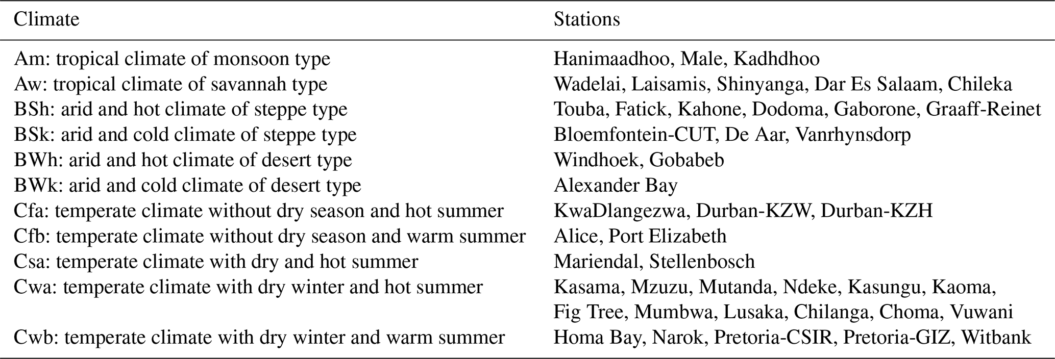
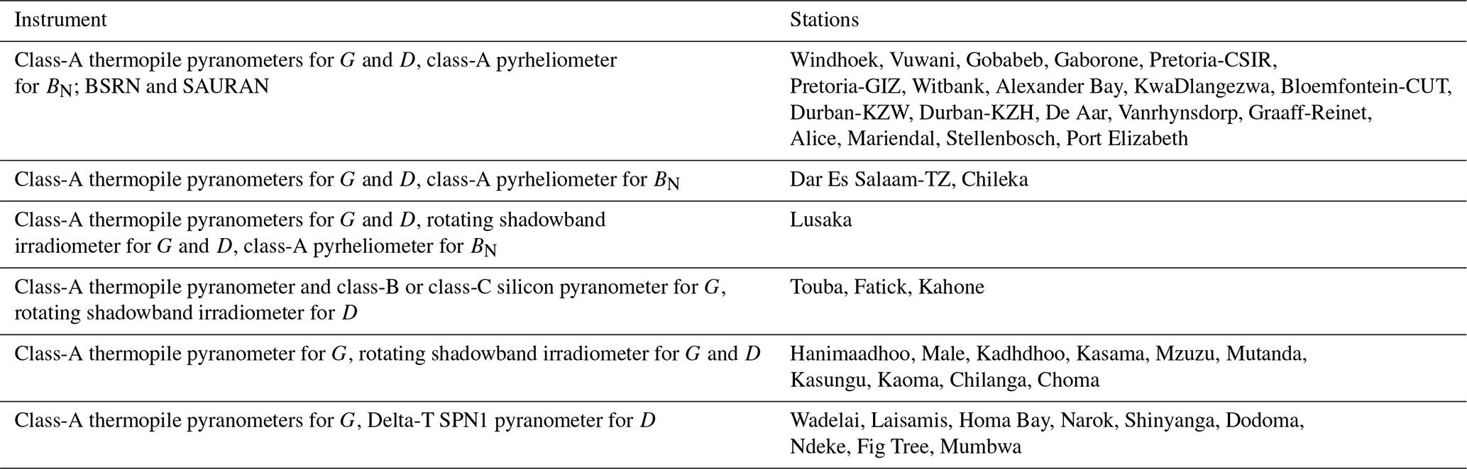
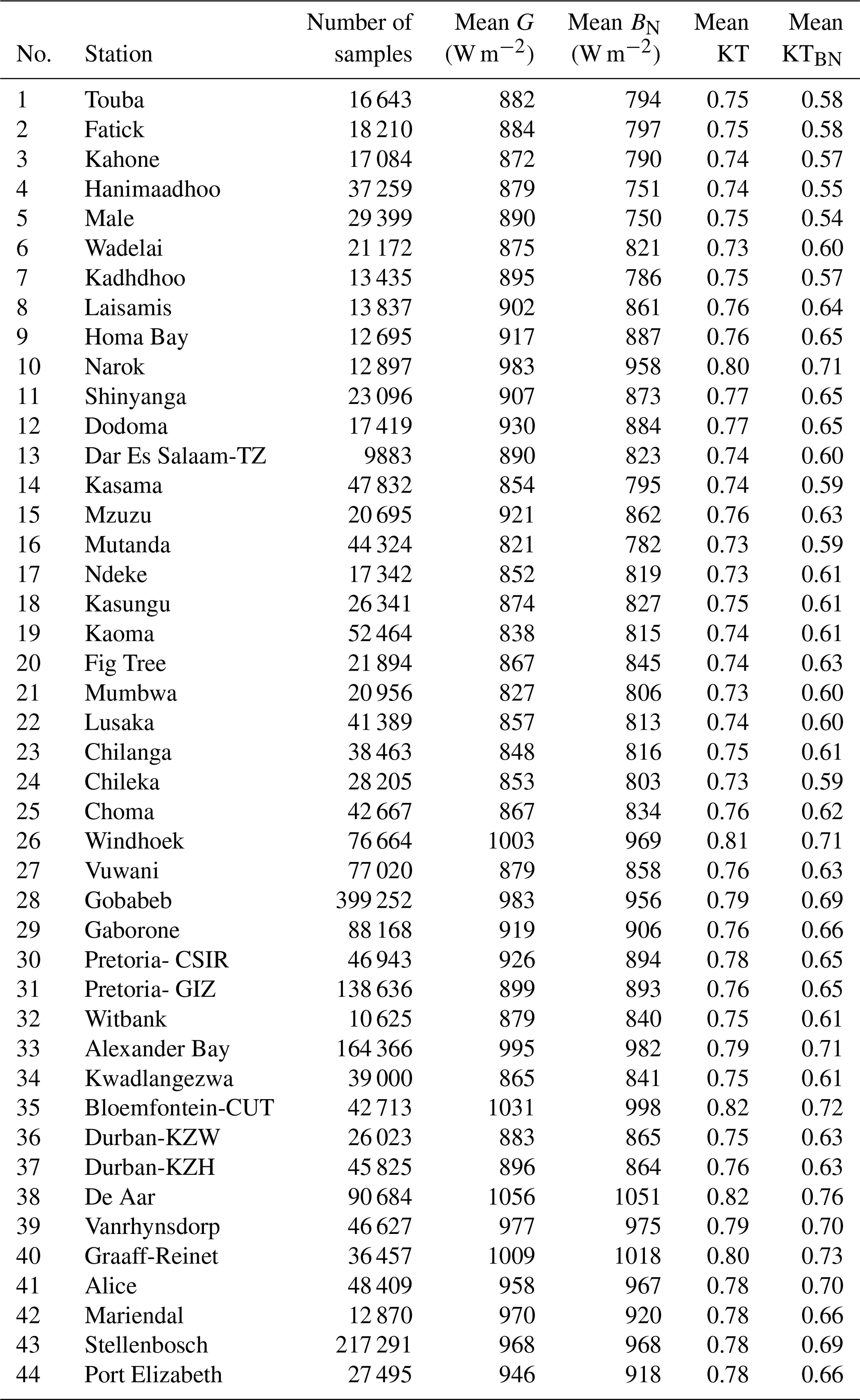
The 1 min ground-based measurements of irradiance received on a horizontal surface, namely the global irradiance G, its diffuse component D, and its direct component B, or the direct component received at normal incidence BN, were collected from several networks offering more than 50 sites for periods ranging from 2010 to 2020, depending on the site. As explained later, the measurements were screened for plausibility and only those made in clear-sky conditions were kept. Additional constraints on the minimal number of selected measurements during each year led to a restricted set of 44 stations. These stations are listed in Table 1 and a map is drawn in Fig. 1. Retained periods of measurements are discussed later. Table 2 lists the Köppen–Geiger climate type for each station according to Peel et al. (2007), while Table 3 lists the instruments used at each station.
The stations Gobabeb (Namibia) and De Aar (South Africa) belong to the Baseline Surface Radiation Network (BSRN, Ohmura et al., 1998) spread throughout the world. BSRN is a project of the World Climate Research Programme and maintains the highest standards in shortwave radiation measurements (Roesch et al., 2011; Vuilleumier et al., 2014). These stations are equipped with class-A (formerly secondary-standard) thermopile pyranometers, with one including a rotating shadow ball, to separately measure G and D with a regular sampling of 1 min and pyrheliometers to measure BN.
SAURAN uses thermopile pyranometers and pyrheliometers similar to those in the BSRN for measuring G, D, and BN every 1 min (Brooks et al., 2015). A total of 19 stations in southern Africa, one in Namibia and one in Botswana, are included in the study.
The remaining stations are financially supported by the World Bank Group apart from four stations supported by the Maldivian corresponding local airports (Hanimaadhoo, Male, and Kadhdhoo), five stations supported by the Zambian Agricultural Research Institute (Kasama, Mutanda, Kaoma, Chilanga, and Choma), one supported by the University of Zambia (Lusaka), one supported by the Malawian University of Mzuzu (Mzuzu), and two supported by the Malawian Ministry of Natural Resources, Energy and Mining (Kasungu and Chileka). All are operated by companies. The instruments used at these stations are diverse and are reported in Table 3. All stations are equipped with at least one class-A thermopile pyranometer, which provides time series of G. A few stations comprise two class-A pyranometers for G. In these cases, we have arbitrarily selected the time series measured by the pyranometers labeled number 1 by the operator in the description of the station. It could have been possible to compare the two datasets but we had no means to decide which one to keep as we did not have all necessary information on the day-to-day operation of each instrument. This could be best done by the site operator. In other cases, stations are equipped with two instruments measuring G. In these cases, we kept the dataset acquired with the most precise instrument, e.g., class-A instrument.
At most stations supported by the World Bank Group, the diffuse component D is provided by either rotating shadowband irradiometers, which measure G and D almost simultaneously on a horizontal plane every 1 min, or Delta-T SPN1 pyranometers, which comprise seven thermopiles and measure G and D simultaneously. In both cases, the direct component on a horizontal plane B is deduced from G and D by the closure equation: . For the sake of the comparison with the other stations, B is converted into BN by dividing B by cos(θS), where θS is the solar zenithal angle and is computed here with the SG2 algorithm (Blanc and Wald, 2012).
Table 1Description of measuring stations used for validation, ordered by decreasing latitude.
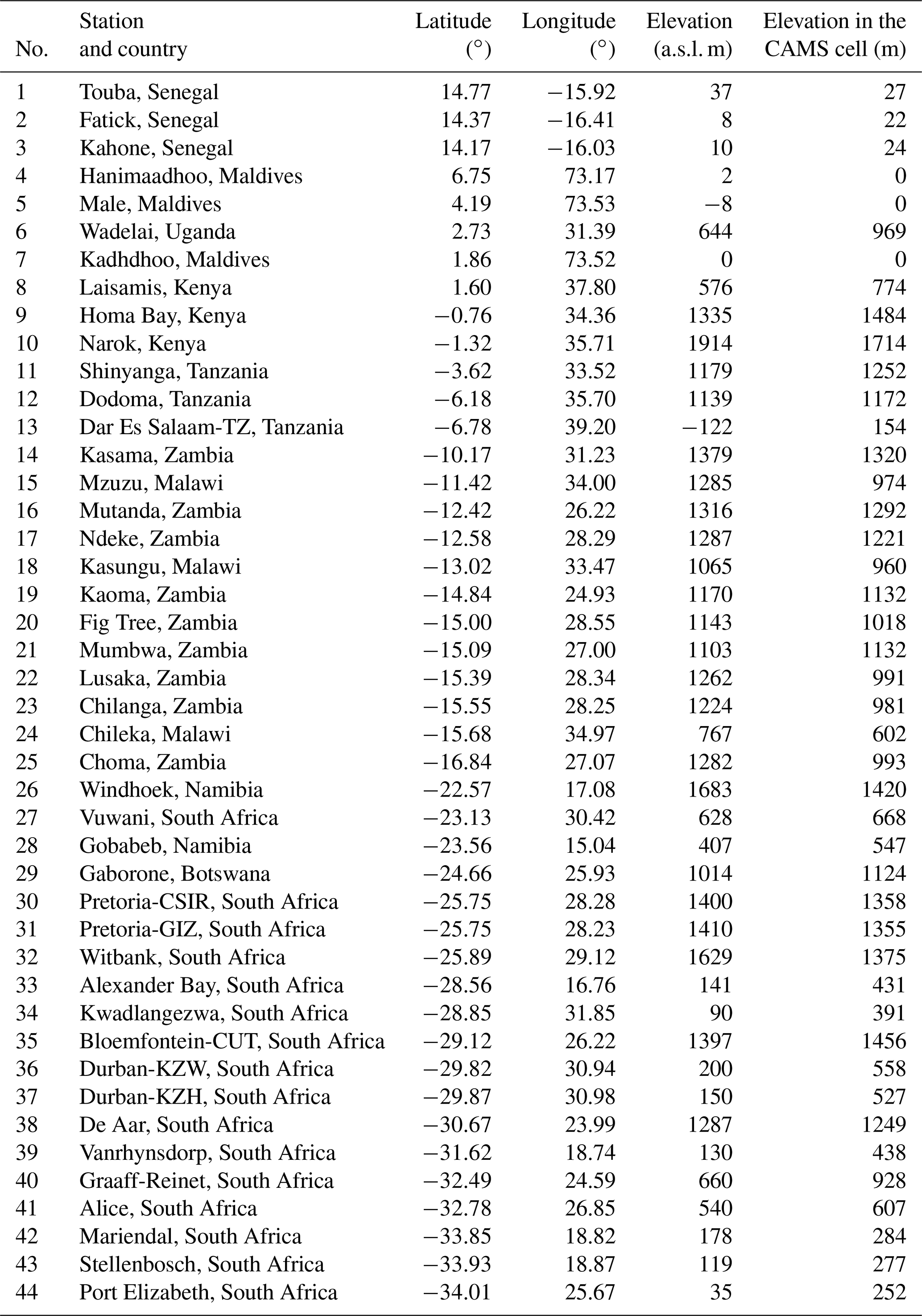
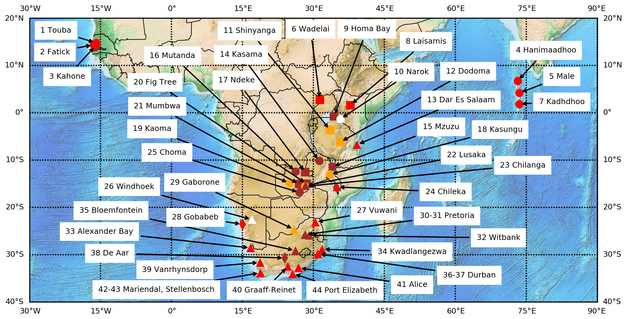
Figure 1Map of the stations. Diamonds are for the BSRN stations, and triangles are for the other stations equipped with pyrheliometers. Circles and squares denote stations equipped with rotating shadowband irradiometers and with Delta-T SPN1 instruments, respectively. Red means an elevation less than 900 m. Orange means an elevation between 900 and 1200 m, brown an elevation between 1300 and 1600 m, and white an elevation greater than 1700 m. Numbers refer to the rank of the station in Table 1. The orographic basemap is under the public domain and is from the Etopo1 dataset from the National Oceanic and Atmospheric Administration of the United States of America.
Table 2List of Köppen–Geiger climate types and corresponding stations, according to Peel et al. (2007).
The World Meteorological Organization (WMO, 2018) sets recommendations for achieving a given accuracy in measuring solar radiation. Each element of a measurement system contributes to the final uncertainty of the data, and the accuracy of solar radiation measurements made at ground stations depends on the radiometer specifications, proper installation and maintenance, data acquisition method and accuracy, calibration method and frequency, location, environmental conditions, and possible real-time or a posteriori adjustments to the data (Sengupta et al., 2021). The WMO document clearly states that “good quality measurements are difficult to achieve in practice, and for routine operations, they can be achieved only with modern equipment and redundant measurements.” In the WMO document, the typical relative uncertainty (95 % confidence level) of measurements of good quality is 8 % for G and D and 2 % for BN with a minimum uncertainty of approximately 17 W m−2 for the latter. The uncertainty targets are more stringent for BSRN measurements: 2 % for G and D and 0.5 % for BN (Ohmura et al., 1998). A very detailed analysis of the uncertainty of measurements made at the BSRN station of Payerne, Switzerland, was performed by Vuilleumier et al. (2014). They reported that the target can be achieved for G and D but not for BN for which the uncertainty is approximately 1.5 %. As for rotating shadowband irradiometers, Wilbert et al. (2016) made a detailed analysis of the uncertainty of measurements acquired by a very well-maintained instrument at the Plataforma Solar de Almería (PSA) station in Spain. They found that the effects of the correction functions, including the spectral irradiance errors, are significant and wrote that uncertainties for corrected 1 min data are estimated to be 2.2 % for G and 3.2 % for BN for both G and BN greater than 300 W m2. In the more general case, Sengupta et al. (2021) report uncertainties of 4 % for G and 5 % for BN. As for the Delta-T SPN1 pyranometer, the uncertainty given by the manufacturer is 8 % for G and D with a minimum uncertainty of approximately 10 W m−2. However, biases have been found as a function of θS and uncertainties may be greater than those given by the manufacturer (Badosa et al., 2014). Möllenkamp et al. (2020) found that monthly recalibration of the instrument against a pyrheliometer significantly reduces the uncertainty.
2.2 Checking the plausibility of the measurements
All the measurements have a temporal resolution of 1 min. Some were flagged by the station operators after a quality check, and only those flagged as non-suspicious were retained. We have performed an additional plausibility check on the data whose aim is not to question the quality flags provided by the station operators, but to check that we made no error in downloading the data and handling them. The tests used here originate from several articles; they are summarized in Korany et al. (2016) and Wald (2021) and reported here for the sake of clarity. The plausibility tests check whether the measurements exceed physically possible and extremely rare limits as well as the consistency between the coincident measurements of G, D, and BN. Let E0N and E0 denote the solar radiation impinging at the top of the atmosphere at normal incidence and on a horizontal surface, respectively, with E0=E0N cos(θS). At any time and any site, E0N and θS are computed by means of the SG2 algorithm (Blanc and Wald, 2012). The tests comprise several constants (given here in W m−2).
The tests based on physically possible limits are as follows.
The tests based on extremely rare limits are as follows.
The tests on consistency between independent measurements are only applied if G>50 W m−2. If G and D are given by two independent instruments, the test is as follows.
If G, D, and BN are given by three independent instruments, the test is as follows.
Suspicious or erroneous measurements were flagged and then removed from the dataset. Then, time series of the retained measurements were plotted together with the corresponding irradiances at the top of the atmosphere, and a visual check was performed to detect and scrutinize outliers that are possibly rejected. In addition, we have put one more constraint on measurements. Since the lowest values can be noise and are therefore insignificant in a validation process, any measurement should be greater than a minimum significant value. If it was not, the measurement was removed from the dataset. The thresholds were selected in such a way such that there is a 99.7 % chance that the actual irradiances G, D, and BN are significantly different from 0 and that they can be used for the comparison. Based on the uncertainty of good-quality measurements of BN as reported by the WMO (2018), the threshold was set to 1.5 times the minimum uncertainty, i.e., 26 W m2 for BN. The WMO document does not give any minimum uncertainty for G or D, and the thresholds were arbitrarily set to 30 W m−2 for both.
2.3 Estimates provided by the McClear service
The McClear model (Lefèvre et al., 2013; Gschwind et al., 2019) is built on abaci, also known as look-up tables, by means of the radiative transfer model libRadtran (Emde et al., 2016; Mayer and Kylling, 2005) based on the most improved Kato et al. (1999) approach (katoandwandji as named in libRadtran, Wandji Nyamsi et al., 2014, 2015). It accurately reproduces G, D, B, and BN computed by the libRadtran reference under clear-sky conditions with a computational speed approximately 105 times greater (Lefèvre et al., 2013), thus offering the opportunity of delivering time series of clear-sky irradiances at a given site within a few seconds. To better exploit this advantage, and though it can be used as a stand-alone model, McClear is often exploited in combination with inputs from CAMS and other sources as a web service freely delivering irradiances at the ground level for any period from 2004 until 2 d ago with different temporal summarizations (1 min, 15 min, 60 min, 1 d, 1 month) at any site in the world. In this sense, McClear is more of an online service than a classic clear-sky model (Cros et al., 2013).
For the sake of conciseness, we refer the reader to Gschwind et al. (2019) for details on the model and on the sources of data automatically used by the McClear service besides the period of time, summarization, and geographical location usually provided by users.
Version 2 was introduced in 2013 to partly palliate several discontinuities in space observed in outputs. A greater step was made with version 3 that removed several artifacts, including discontinuities in space and time in irradiance. Comparisons were performed between measurements made at 11 BSRN sites and estimates of G, D, B, or BN from both McClear-v2 and McClear-v3 services by Gschwind et al. (2019), who found similar results between the three versions. It follows that works dealing with the v1, v2, or v3 can be compared, as we will do in Sect. 6.
McClear irradiances are freely accessible by machine-to-machine calls to the web service McClear on the SoDa Service (Gschwind et al., 2006, https://www.soda-pro.com/, last access: 11 August 2022) or manually through a web interface. In the verbose mode, the flow returned by the service contains 1 min values of readings from CAMS resampled to the selected location by spatial bilinear interpolation and resampled in time by linear interpolation, namely the optical depth of aerosols at 500 nm and the total column contents in water vapor and ozone. It also contains 1 min values of θS calculated with the SG2 algorithm, irradiances at the top of atmosphere and at ground level, and ground albedo, calculated by McClear. This mode was conveniently exploited for the collection of McClear estimates for the same periods and same locations as the 1 min ground measurements.
3.1 Screening of cloudless instants
Several algorithms for detecting clear-sky instants within a series of measurements to separate the cloud-contaminated instants from the cloud-free ones have been published (see, e.g., Bright et al., 2020; Calbó et al., 2001; Ellis et al., 2019; Long and Ackerman, 2000; Reno and Hansen, 2016). Similarly to the developers of the McClear service (Lefèvre et al., 2013; Gschwind et al., 2019), we used the algorithm of Lefèvre et al. (2013) here. The possible influence of the algorithm on results is discussed in Sect. 6.
Let E0N and E0 denote the solar radiation impinging at the top of the atmosphere at normal incidence and on a horizontal surface, respectively. The clearness index KT, direct normal clearness index KTBN, and corrected clearness index KTcor (Perez et al., 1990) are respectively defined as
where m is the air mass defined by Kasten and Young (1989):
where θS is the solar zenithal angle expressed in degrees, and p and p0 are respectively the pressure at the site under consideration and that at sea level. The ratio of pressures can be approximated as
where z is the elevation above sea level: 8435.2 m. KT is equal to the global transmissivity of the atmosphere, or, alternatively, atmospheric transmittance or atmospheric transmission when there is no reflection of the ground. KTcor exhibits less dependence with θS than KT (Perez et al., 1990).
The first filter in the Lefèvre et al. algorithm is a restriction on D with respect to G since B is usually prominent in a cloud-free atmosphere:
Only measurements that satisfied the first filter were retained. The second filter investigates the temporal fluctuation of the corrected clearness index KTcor since this amount must be stable for numerous hours in a cloudless atmosphere. The first step of this filter is to retain only periods with enough measurements that have passed the first filter. A given instant t, expressed in minutes, is kept only if at least 30 % of the 1 min observations in both intervals [t−90 min, t] and [t, t+90 min] have been retained after the first filter. An instant is considered clear if the standard deviation of KTcor in the interval [t−90 min, t+90 min] is less than a threshold empirically set to 0.02. Only these 1 min clear-sky instants were retained for the validation, and all computations in the following were made with this subset of clear-sky instants. Because of the second filter, all retained instants are within [sunrise + 90 min, sunset −90 min].
3.2 Selection of periods, number of samples, and means of measurements
Apart the daily cycle of the solar zenithal angle, G in cloudless conditions exhibits only one yearly noticeable cycle (Bengulescu et al., 2017, 2018), though the occurrence of cloud-free conditions varies with seasons. Hence, the year is an appropriate period for the validation of the McClear service. At a given station, a year is declared valid if the number of clear-sky instants is greater than a threshold arbitrarily set to 9000. This threshold is large enough to account for various situations and is of the same magnitude as the mean number of measurements used at each station in Lefèvre et al. (2013). In addition, using yearly periods allows the analysis of changes in statistical indicators with time.
A few exceptions to the general rule were made in order to account for local conditions and to retain the greatest possible number of stations and measurements in the analysis. Namely, station nos. 1, 2, and 3 have only data from January to September in 2017. A pseudo-year 2017 was created at these stations, consisting of 12 consecutive months spanning over 2 years: October 2016 to September 2017. Similarly, a pseudo-year 2018 was created at the stations Ndeke (no. 17), Fig Tree (no. 20), and Mumbwa (no. 21) consisting of 12 consecutive months spanning from September 2017 to August 2018. Figure 2 (left) gives the years retained at each station for G and BN as well as the number of samples in each year. Table 4 reports the number of samples kept for validation at each station for all retained years. Most stations exhibit 1 or 2 years of data. Many SAURAN stations have more than 2 years of data. Stations Stellenbosch (no. 43), Gobabeb (no. 28), and Pretoria-GIZ (no. 31) have the longest records in this selection with 9, 8, and 7 years, respectively.
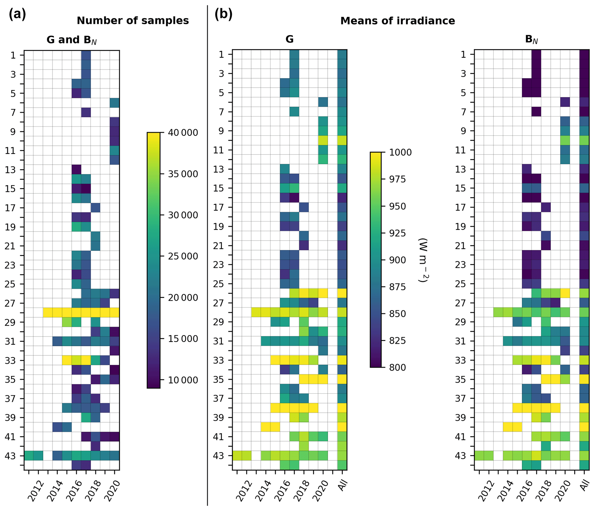
Figure 2Number of retained measurements (a) and means of G and BN (b) at each station for each year. Also reported are the means for G and BN for the whole period (All). Numbers refer to the rank of the station in Table 1.
Figure 2 (center and right) provides in graphical form the means of G and BN for each year and for the whole period. The latter are also given in Table 4, as are the means of KT and KTBN. As stations are ordered by decreasing latitudes, Fig. 2 shows an overall latitudinal trend in G, BN, KT, and KTBN, which tend to increase southwards. The trend is blurred by the different elevations, climates, total water vapor content, aerosol loading, and possibly instrumentation for BN. As a whole, the mean of G is almost constant from station no. 1 to station no. 7 then increases with a local maximum at Narok (no. 10), likely because of its high elevation of 1914 m. Then, it exhibits a kind of trough at stations (nos. 14–23, 25, 27) that experience the Cwa climate and show lower means of G than the others, though their elevation is often greater than 1000 m. The behavior is more confused at station nos. 26–44, though the mean tends to increase southwards with local maxima at Windhoek (no. 26), Bloemfontein-CUT (no. 35), and De Aar (no. 38), likely due to their elevation greater than 1300 m. Variables other than elevation intervene. For example, Pretoria (nos. 30–31) and Witbank (no. 32) have elevations greater than 1400 m and exhibit lower means of G than Alexander Bay (no. 33) and Graaff-Reinet (no. 40), whose elevations are respectively 141 and 660 m. The three former experience the temperate Cwb climate, while the two latter experience arid BWk and BSh climates. The minimum of BN is observed at Hanimadhoo (no. 4) and Male (no. 5). The mean of BN is often close to the mean of G, though it is less. Exceptions are observed at the stations in Senegal and Maldives where BN is much less than G. As BN and G are close at the other stations, BN exhibits behavior similar to that of G.
As a whole, means of G and BN in cloudless conditions are fairly constant throughout years at a given station with changes from year to year often less than 3 % of the yearly average, i.e., approximately 30 W m−2. Magnitudes of changes are partly due to differences in atmospheric conditions and partly due to differences in the number of data available in each year and their distribution within the year. A special look at the very close stations, namely the two stations no. 30 (Pretoria-CSIR) and 31 (Pretoria-GIZ), less than 4 km apart having the same elevation, and the stations Durban-KZW (no. 36) and Durban-KZH (no. 37) that are 7 km apart, with a difference in elevation of 50 m (200 m vs. 150 m), reveals that the yearly mean of BN exhibits almost no difference between the closest stations in a given year. The differences are 11, 5, and 23 W m−2 in 2018, 2019, and 2020, respectively, at Pretoria and 10 and 1 W m−2 in 2016 and 2017, respectively, at Durban. This is also true for G at Durban: the differences are respectively 21 and 12 W m−2 in 2016 and 2017. At Pretoria, the differences in G may be more pronounced depending on the year: 58, 17, and 59 W m−2 in 2018, 2019, and 2020.
The mean clearness index KT is between 0.73 and 0.82 (Table 4). The greatest values are observed at elevated sites, with the exception of no. 40 (KT = 0.80), though its elevation is only 660 m. The clearness index KTBN is between 0.54 and 0.76. Like for KT, the greatest values are found at elevated sites, with the exceptions of Alexander Bay (no. 33, KTBN=0.71) and Graaff-Reinet (no. 40, KTBN=0.73) of low elevation: 141 and 660 m, respectively.
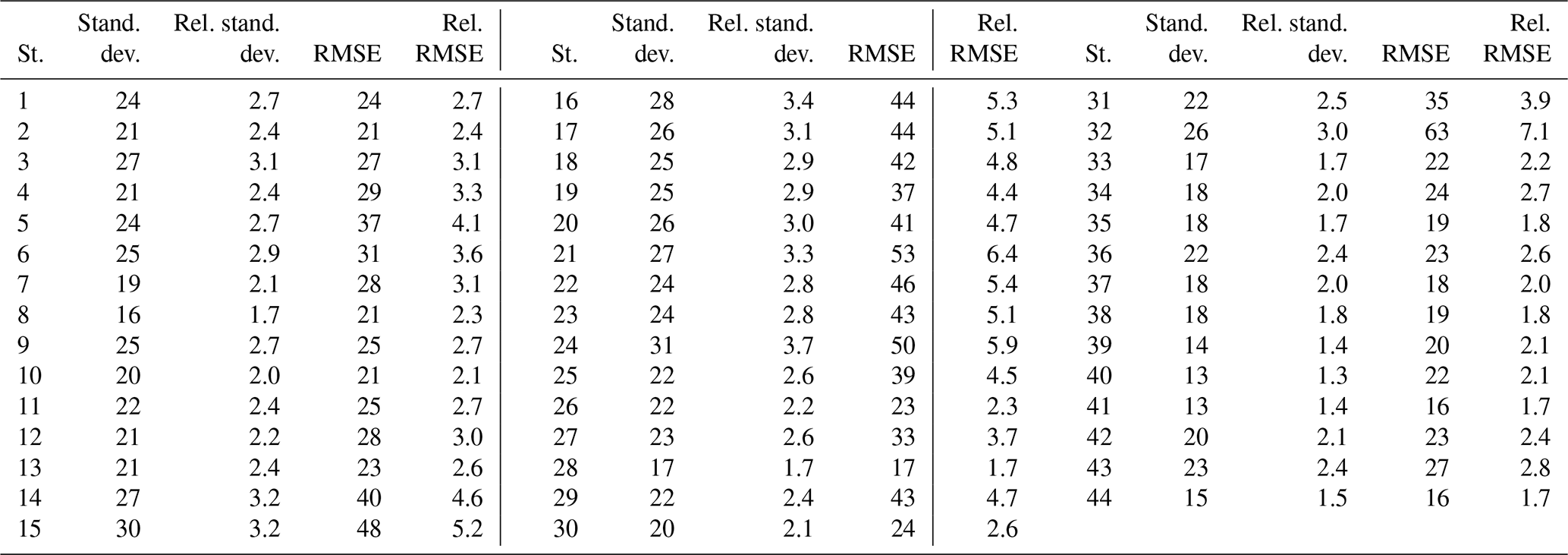
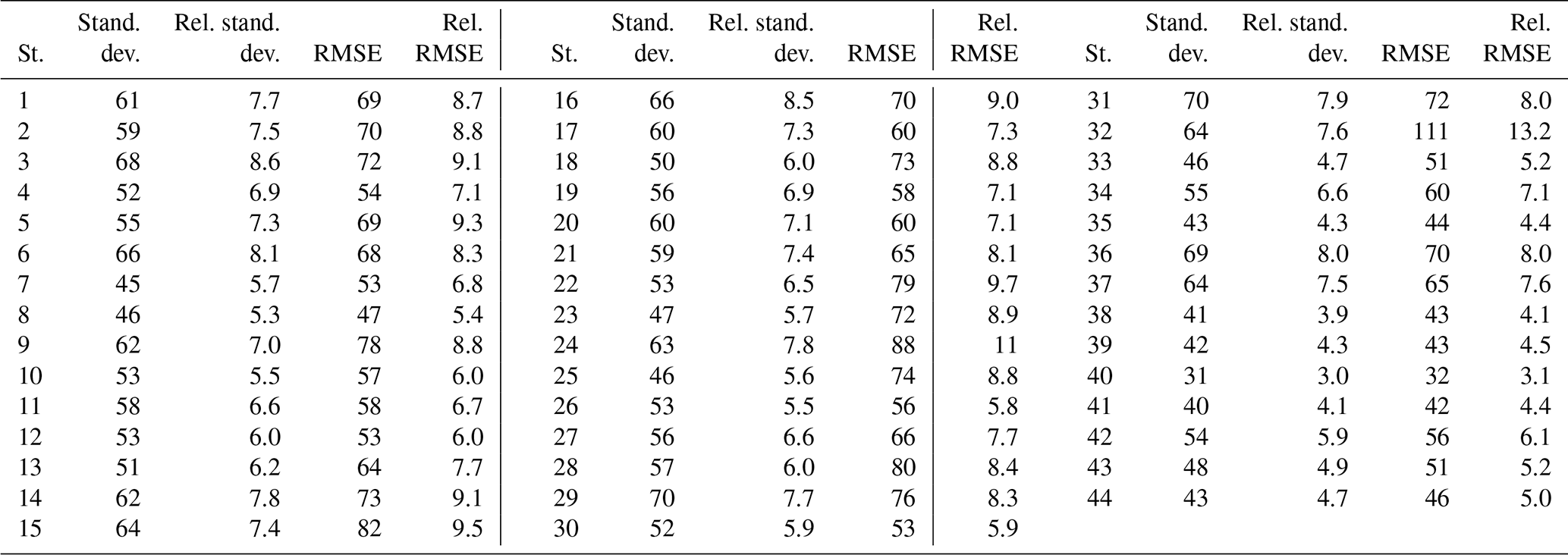
Table 4Number of samples for validation, along with the means of G, BN, KT, and KTBN at each station for the ensemble of retained years.
3.3 Methodology of validation
The validation was performed by computing the differences between the McClear estimates and the measurements for coincident instants and location, for each year, and for the ensemble of years. The differences were summarized by their mean, known as the bias or mean bias error, their standard deviation, and the root mean square error (RMSE). Relative biases, relative standard deviations, and relative RMSEs at each station were expressed with respect to the means of the measurements for the corresponding period at this station. The Pearson correlation coefficients, slopes, and offsets of the least-squares fitting lines were computed as were the ratios of estimates to measurements and the ratios of variances of estimates to those of measurements. Several graphs were also drawn such as 2D histograms of measurements and estimates, histograms of each dataset, and histograms of differences as well as box plots of ratios and differences as a function of θS, total column contents in ozone and water vapor, and optical depth of aerosols at 550 nm.
These operations were performed for G, BN, KT, and KTBN at each station for the whole dataset and also for subsets of data built for different years, different classes of θS, different classes of readings from CAMS, namely optical depth of aerosols at 500 nm as well as total column contents in water vapor and ozone, and different classes of ground albedo read from McClear outputs. Graphs were drawn to assess the influence of these quantities. Results were analyzed as a function of the station, latitude, climate, elevation, year, means of irradiance or clearness index, variances of the measurements, instruments, and even operators to evidence possible trends.
Since correlation coefficients close to 1 mean that measurements and estimates vary similarly in time and slopes close to 1 mean that the amplitudes of the variations are similar, expectations are correlation coefficients and slopes of the fitting lines both close to 1. Biases are expected to be close to 0 and ratios of variances are expected to be close to 1. A bias greater than 0 or a ratio of variances greater than 1 would mean an overestimation of the mean and variance. Knowing that the relative standard deviation is half the relative uncertainty assuming a Gaussian distribution of errors, the expectations about the relative standard deviation depend on the relative uncertainty of the measurements and are based on the hypothesis that the McClear outputs, excluding possible bias, meet the good-quality standard of the World Meteorological Organization (WMO, 2018). Using a bulk approach, we have assumed that the square of the uncertainties in this validation is the quadratic sum of the uncertainties of the McClear estimates and of the uncertainties of the measurements (see e. g., Sengupta et al., 2021, for more complex approaches). The relative standard deviation of the errors in this validation, σ, is given by
where σinstrument is half the relative uncertainty of the instrument and σMcClear is half that of the McClear outputs. σMcClear is hypothetically set to 4 % for G and 1 % for BN as discussed in Sect. 2.1. At BSRN stations, σinstrument is set to 1 % for G and 1 % for BN. At other stations, σinstrument is set to 4 % for G. As for BN, σinstrument is set to 1 % at stations equipped with pyrheliometers, 2.5 % at stations equipped with rotating shadowband irradiometers, and 4 % at stations equipped with SPN1 instruments. Table 5 provides the expectations for σ depending on the instruments. σ should be less than or equal to the corresponding limits in Table 5 if the McClear outputs, excluding bias, meet the good-quality standard of the World Meteorological Organization.
Table 5Expectations for the relative standard deviation of errors σ (%).
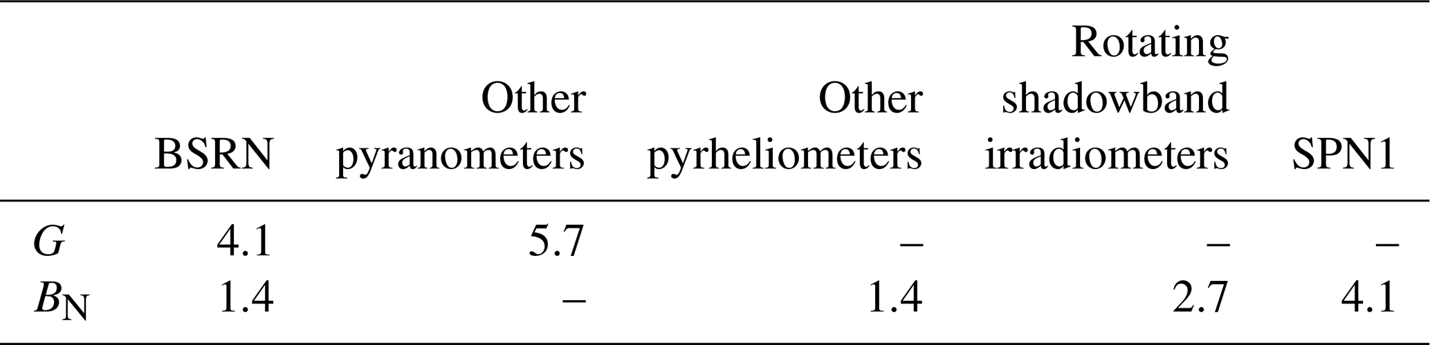
Figure 3 exhibits examples of the 2D histograms for G and BN at the BSRN station Gobabeb (no. 28). At this station, the measurements of G are reproduced well by the McClear service (left graph). The cloud of points is elongated well along the identity line with very limited scattering. The scattering of points is more pronounced for BN (right graph). Other 2D histograms at each station are available in the Supplement as are many other graphs, including for clearness indices KT and KTBN.
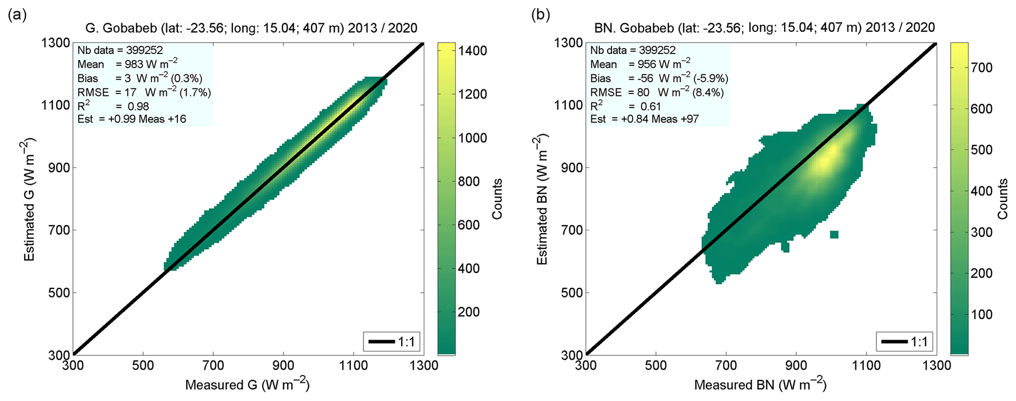
Figure 32D histograms between measurements (horizontal axis) and McClear-v3 estimates (vertical axis) for G (a) and BN (b) at the BSRN station Gobabeb (no. 28). The color indicates the number of pairs in each class.
4.1 Means and variances for G
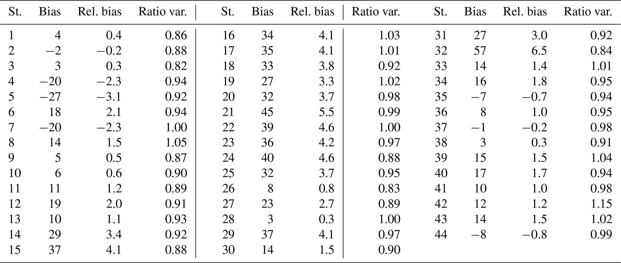
Table 6 reports the bias, the relative bias, and the ratio of variances at each station for G. Graphs in Appendix A exhibit the changes with years of the statistical quantities for G and BN. The leftmost graphs in Figs. A1 and A2 respectively exhibit the bias and relative bias for G at each station for each year and for the whole period. The bias ranges between −27 and 57 W m−2. If these extremes are removed, the bias lies within [−20, 45] W m−2, i.e., [−2.3, 5.5] %, with a mean of 16 W m−2 (1.8 %). The bias is most often positive (Fig. A1) and half of the stations exhibit small bias in the range [−15, 15] W m−2. The bias shows a strong dependency with climate and with station to a lesser extent (Table 6 combined with Table 2). The bias is large and negative at the three stations in the Maldives Archipelago, experiencing a tropical climate of monsoon type (Am) (Table 6). On the contrary, stations in the tropical climate of savannah type (Aw, nos. 6, 8, 11, 13, 24) offer a positive bias from 10 to 18 W m−2, with the exception of the southernmost one (Chileka, no. 24, 40 W m−2). The bias in arid climates (BSh, BSk, BWh, BWk) ranges between −7 and 15 W m−2, with the exception of the elevated station no. 12 (19 W m−2) in the BSh climate and the two southernmost stations no. 29 (37 W m−2) and no. 40 (17 W m−2). The stations in temperate climates without a dry season (Cfa, Cfb, nos. 34, 36–37, 41, 44) or with a dry and hot summer (Csa, nos. 42–43) exhibit biases from −8 to 16 W m−2. Those in temperate climates with a dry winter and hot summer (Cwa: nos. 14–23, 25, and 27) exhibit the greatest biases in the interval [23, 45] W m−2, i.e., [2.7, 5.5] %. Stations in temperate climates with a dry winter and warm summer (Cwb, nos. 9–10, 30–32) exhibit high variability in bias from 5 W m−2 (0.5 %) to 57 W m−2 (6.5 %). Both BSRN stations (no. 28 Gobabeb, BWh, and no. 38 De Aar, BSk) exhibit a bias of only 3 W m−2 (Table 6). Changes in bias from year to year at a given station are less than 10 W m−2 in absolute value (approx. 1 % in relative value) in 84 % of cases (Fig. A1, left). Relative differences slightly greater than 1 % are observed for the same year at pairs of close stations in Pretoria (nos. 30–31) and Durban (nos. 36–37) (Fig. A2, left).
The ratio of variances ranges between 0.82 and 1.15 (Table 6). If these extremes are excluded, the ratio lies in the interval [0.83, 1.05] with a mean of 0.95. It is often less than 1, which means an underestimation of the variance. About half of the stations (45 %) exhibit ratios between 0.95 and 1.05 (Table 6). The link with elevation is unclear, though stations of elevation greater than 1300 m have ratios less than 0.95 whatever the climate. There is a clear link with climates (Table 6 combined with Table 2). The ratios are often less than 0.95 in tropical climates (Am, Aw) and arid climates of steppe type (BSh, BSk). They are closer to 1 in arid climates of desert type (BWh, BWk) and temperate climates (Cfa, Cfb, Csa, Cwa). An exception is the temperate climate Cwb whose stations are above 1300 m with ratios less than 0.93. Changes in the ratio of variances from year to year at a given station range from −0.28 to 0.30 but are within the interval [−0.05, 0.05] in 63 % of the cases (not shown). Changes are less than 0.05 in absolute value at pairs of close stations for the same year: Pretoria (nos. 30–31) and Durban (nos. 36–37).
In summary, there are links between elevation and climates and between the bias and ratio of variances. The variance is underestimated at elevation greater than 1300 m whatever the climate. In tropical climates, the variance of G is underestimated, while the mean is underestimated (Am) or overestimated (Aw). In arid climates, McClear fairly correctly estimates the mean. It fairly correctly estimates the variance in climates of desert type (BWh, BWk) and underestimates it in climates of steppe type (BSh, BSk). In temperate climates, the variance is correctly estimated with the exception of stations in Cwb climates due to their high elevation. The mean is fairly correctly estimated in Cfa, Cfb, and Csa and is strongly overestimated in Cwa and Cwb.
Table 6Bias (in W m−2), relative bias (in %), and ratio of variances for G at each station.
4.2 Means and variances for BN
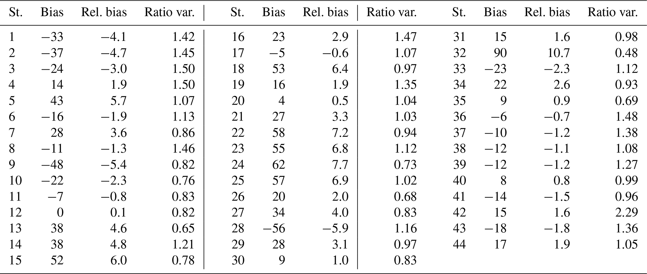
Table 7 reports the bias, the relative bias, and the ratio of variances at each station for BN. The rightmost graphs in Figs. A1 and A2 respectively exhibit the bias and relative bias for BN at each station for each year and for the whole period. The bias ranges between −56 and 90 W m−2. If these two extremes are removed, the bias lies in a narrower interval of [−48, 62] W m−2, i.e., [−5.4, 7.7] %, with a mean of 11 W m−2 (1.4 %). The bias is positive at 27 stations (64 % of the total) (Table 7), and 13 stations exhibit small relative bias in the range [−1.5, 1.5] %, i.e., 29 % of the stations. The influence of the climate or elevation is much less marked than for G for both the bias and ratio of variance. One may note that stations located in climates Am and Cwa exhibit positive biases that are among the greatest.
Changes in bias from year to year at a given station are less than 10 W m−2 in absolute value in 40 % of cases (approx. 1 % in relative value) (Fig. A1, right). Relative differences around 1 % are observed for the same year at pairs of close stations in Pretoria (nos. 30–31) and Durban (nos. 36–37) (Fig. A2, right). The widths of the intervals [−48, 62] W m−2 for the bias throughout the stations and [−5.4, 7.7] % for the relative bias are 110 W m−2 and 13.1 %, respectively (Table 7): there is a large variation of the bias within the set of stations.
The ratio of variances ranges between 0.48 and 2.29 (Table 7). If these extremes are excluded, the ratio lies in the interval [0.65, 1.50] with a mean of 1.07. The ratio exceeds 1 at 24 stations (overestimation) and is less than 1 at the 20 others. Nine stations exhibit ratios between 0.95 and 1.05. Changes in the ratio of variances from year to year at a given station range from −0.61 to 0.98 and are within the interval [−0.10, 0.10] in 20 % of the cases only (not shown). Changes are less than 0.1 in absolute value at pairs of close stations in Pretoria (nos. 30–31) and Durban (nos. 36–37) for the same year. The width of the interval of variations in the ratio throughout the stations is 0.85, i.e., 79.1 % relative to the middle of the range (Table 7). It can be concluded that McClear tends to overestimate both the means and variances of BN, though these conclusions depend on the stations as the bias and the ratio of variances can hardly be considered constant in time and space.
Table 7Bias (in W m−2), relative bias (in %), and ratio of variances for BN at each station.
4.3 Correlation coefficients and slopes of the least-squares fitting lines for G
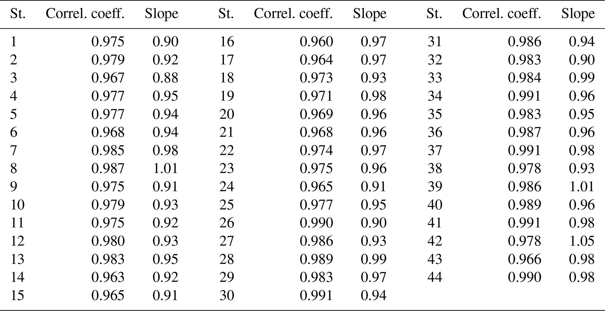
Table 8 reports the correlation coefficients and slopes of the least-squares fitting lines for G at each station, while Fig. A3 (left part) exhibits the correlation coefficients at each station for each year and for the whole period. The McClear estimates for G correlate very well with the measurements at all stations. This was expected because of the strong influence of the solar zenithal angle. Correlation coefficients are between 0.960 and 0.991 (Table 8) and are greater than 0.970 at 35 stations (80 % of the stations). The greater the mean KT, the greater the correlation coefficient (Table 8 combined with Table 4). Slopes are between 0.88 and 1.05 and between 0.95 and 1.05 at 25 stations (57 % of the stations) (Table 8). Correlation coefficients vary very little throughout years at a given station: changes are less than 0.02 (Fig. A3, left). In addition, they are very close to each other at each station for both pairs of close stations in Pretoria (nos. 30–31) and Durban (nos. 36–37) for the same years (Fig. A6, left). This is also true for the slopes with relative changes from year to year less than 10 %. The correlation coefficients and the slopes are very close to each other within the same climatic area whatever the elevation of the stations (Table 8 combined with Table 2). It can be concluded that the correlation coefficients and the slopes have little variation in time and can be considered constant in time and at close locations.
The width of the interval [0.960, 0.991] of the correlation coefficients throughout the stations is 0.031, i.e., 3 % relative to the middle of the range (Table 8). This is very small: it can be reasonably assumed that the correlation coefficient varies very little in space. If the minimum in slope is excluded, the slopes lie in the interval [0.90, 1.05] whose width is 0.15, i.e., 15 % relative to the middle of the range (Table 8), which means that the spatial variation in slopes is noticeable at mesoscales. We conclude that the minute-to-minute variability in G is reproduced well by McClear at all stations, though there is a tendency at some places to overestimate the smallest irradiances and underestimate the greatest ones, with unpredictable variations of this tendency in space.
Table 8Correlation coefficients (Correl. coeff.) and slopes of the least-squares fitting lines at each station for G.
4.4 Correlation coefficients and slopes of the least-squares fitting lines for BN
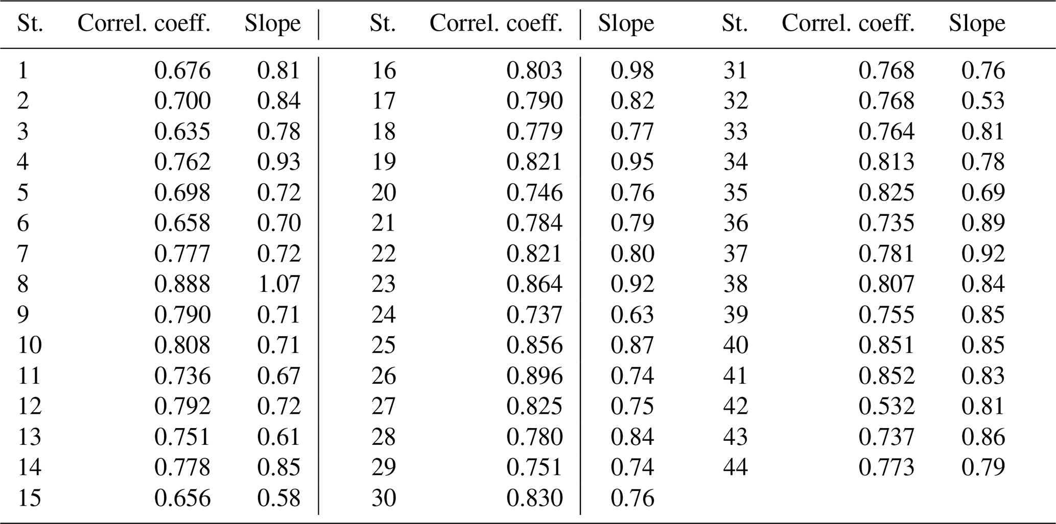
Table 9 reports the correlation coefficients and slopes of the least-squares fitting lines at each station for BN, while Fig. A3 (right part) exhibits the correlation coefficients at each station for each year and for the whole period. The McClear estimates for BN correlate well with the measurements at most stations. The correlation coefficient for BN ranges between 0.532 and 0.896 (Table 9). It is greater than or equal to 0.700 at all stations, except six. Similarly to G, the greater the mean KTBN, the greater the correlation coefficient (Tables 4 and 9). Slopes are less than 1 except at Laisamis (no. 8) and are often close to 0.80 (Table 9). Correlation coefficients for BN may vary or not with years at a given station: changes greater than 0.1 may be observed at several stations (Fig. A3, right). Changes in slope may also be highly variable depending on the station and the year. Correlation coefficients and slopes are constant at short spatial scales: they are very close to each other at each station for both pairs of close stations in Pretoria (nos. 30–31) and Durban (nos. 36–37) for the same years (Fig. A3, right).
The correlation coefficients and slopes vary significantly from one station to the other (Table 9). If the six stations, nos. 1, 3, 5, 6, 15, and 42, are excluded, the correlation coefficient for BN lies in the interval [0.700, 0.896], whose width is 0.196, i.e., 25 % relative to the middle of the range. The change in space in correlation coefficient is important and cannot be neglected. If the minimum in slope (0.53 at no. 32, Witbank) is excluded, the slopes lie in the interval [0.58, 1.07] whose width is 0.49, i.e., 60 % relative to the middle of the range, which is important. If the four smallest slopes are excluded, the slopes vary between 0.67 and 1.07 and the width of the range is now 0.40, i.e., 46 % relative to the middle of the range, which is still large. We conclude that the minute-to-minute variability in BN is reproduced fairly well by McClear at all stations, though there is an overestimation of the smallest irradiances and an underestimation of the greatest ones, with the magnitudes of these being unpredictable in time and space.
Table 9Correlation coefficients (Correl. coeff.) and slopes of the least-squares fitting lines at each station for BN.
4.5 Standard deviations of errors and RMSE for G
Table 10 reports the standard deviation of errors σ, the RMSE, and their values relative to the mean of the measurements at each station for G. The leftmost graphs in Figs. A4 and A5 respectively exhibit the standard deviation of errors and its relative value at each station for each year and for the whole period. The standard deviation ranges between 13 and 31 W m−2, which is a very limited range (Table 10). If these extremes are removed, the standard deviation lies within [13, 30] W m−2, with a mean of 22 W m−2 (2.4 %). This is small, and 37 stations out of 44 report a relative standard deviation less than 3 %. The RMSE for G ranges between 16 W m−2 (1.7 %) and 63 W m−2 (7.1 %). If these extremes are removed, the RMSE lies within [17, 53] W m−2, i.e., [1.7, 6.4] %, with a mean of 31 W m−2 (3.4 %). Similarly to the bias (3 W m−2), the standard deviations of errors at the BSRN stations are very close to each other (17 and 19 W m−2) as is the RMSE (17 and 19 W m−2) (Table 10). One may note a tendency with some climate areas: the smallest standard deviations are found at stations in climates BWh, BWk, Cfa, BSk, Cfb, and Csa and range between 12 and 23 W m−2. Actually, the greater the mean KT, the smaller the standard deviation and the RMSE (Tables 4 and 10). There is a slight trend with latitude, which is likely related to the mean KT as the latter increases as the latitude decreases: the smaller the latitude, the smaller the standard deviation and the RMSE.
Standard deviations of errors vary very little throughout years at a given station (Figs. A4 and A5, left): relative changes are less than 0.5 % in 89 % of cases and less than 1 % in all cases but two. In addition, they are very close to each other at pairs of close stations in Pretoria (nos. 30–31) and Durban (nos. 36–37) for the same years. Similar observations are made for the RMSE as it is a quadratic combination of the standard deviations of errors and the bias. The widths of the intervals [13, 30] W m−2 for the standard deviation throughout the stations and [1.4, 3.4] % for the relative standard deviation are 17 W m−2 and 2.0 %, respectively. This is very small: it can be reasonably assumed that the standard deviation of errors varies very little in space. Due to the influence of the bias, the widths of the RMSE intervals are larger: they are 26 W m−2 and 4.7 %, respectively. The relative standard deviation of errors is less than the expectations listed in Table 5 at all stations: except for the bias, the McClear outputs are compliant with the good-quality standard of the World Meteorological Organization.
Table 10Standard deviations of errors (in W m−2), RMSE (in W m−2), and their values relative to the mean of the measurements (in %) for G at each station.
4.6 Standard deviations of errors σ and RMSE for BN
Table 11 gives the standard deviation of errors σ, the RMSE, and their values relative to the mean of the measurements at each station for BN. The rightmost graphs in Figs. A4 and A5 respectively exhibit the standard deviation of errors and its relative value at each station for each year and for the whole period. The standard deviation for BN ranges between 31 and 70 W m−2 (Table 11). Once theses extremes removed, the standard deviation is within [40, 69] W m−2, i.e., [4.1, 8.0] %, with a mean of 55 W m−2 (6.4 %). The standard deviation is less than 60 W m−2 (∼7 % in relative value) at 31 stations out of 44 (70 % of the total) (Table 11). The RMSE for BN ranges between 32 and 111 W m−2. If these extremes are removed, the RMSE lies within [42, 88] W m−2, i.e., [4.1, 11.0] %, with a mean of 63 W m−2 (7.4 %). There is no trend with climate, though one may note that the smallest standard deviations and RMSEs are observed in climates BSk, BWk, and Cfb. Though less pronounced than for G, the greater the mean KTBN, the smaller the standard deviation and the RMSE (Tables 4 and 11). There is a slight trend with latitude, which is likely related to the mean KTBN as the latter increases as the latitude decreases: the smaller the latitude, the smaller the standard deviation and the RMSE. Finally, the smaller the variance of the measurements, the smaller the standard deviation of errors and the RMSE.
Changes in standard deviations of errors from year to year at a given station are small in most cases as they are less than or equal to 10 W m−2 in absolute value in 84 % of cases (Fig. 7, right). This ratio is 68 % for the RMSE (not shown). The standard deviations of errors and the RMSEs are very close to each other at pairs of close stations in Pretoria (nos. 30–31) and Durban (nos. 36–37) for the same years.
The widths of the intervals [40, 70] W m−2 for the standard deviation throughout the stations and [3.9, 8.5] % for the relative standard deviation are 30 W m−2 and 4.6 %, respectively. They are moderate: it can be reasonably assumed that the standard deviation of errors varies fairly little in space. Due to the influence of the bias, the widths of the RMSE intervals are larger: they are 46 W m−2 and 6.9 %, respectively. The relative standard deviation of errors at any station is always above the expectations listed in Table 5: even excluding the bias, the McClear outputs for BN are not compliant with the good-quality standard of the World Meteorological Organization.
Table 11Standard deviations of errors (in W m−2), RMSE (in W m−2), and their values relative to the mean of the measurements (in %) for BN at each station.
Discrepancies between ground-based measurements and McClear outputs are the result of the combination of uncertainties of several major sources, which are the uncertainties of the measurements already discussed in Sect. 2, the protocol of validation itself, and the errors in the McClear model and its inputs.
5.1 Protocol of validation
The protocol of validation used here is the same as those used in similar studies and is well-known. It presents two drawbacks because it compares quantities that are not exactly comparable in all aspects. McClear provides total irradiance, or more exactly the irradiance integrated over the [240, 4606] nm range used in the Kato et al. (1999) approach, while measurements by pyranometers are taken in a more limited range, often called the broadband range, which is around [285, 2800] nm for pyranometers used in the BSRN, SAURAN, and other networks. Simulations made with the radiative transfer model libRadtran show that the relative contribution of the irradiance in this BSRN spectral range [285, 2800] nm to the total irradiance is around 99 % and depends slightly on atmospheric properties. Hence, by comparing measurements acquired in a BSRN-like interval and McClear estimates of total irradiance, one would expect an overestimation of approximately 1 %, i.e., of the order of 5 W m−2. We have assessed this point for G and B by comparing results published by Lefèvre et al. (2013) and Gschwind et al. (2019). Both works used the same dataset of measurements from 11 BSRN stations filtered for clear-sky instants. For the purpose of the comparison with BSRN measurements, Gschwind et al. (2019) computed two specific BSRN-like v1/v2 and v3 versions of McClear tailored to the BSRN spectral range. Hence, the results of the BSRN-like v1/v2 in Tables 5 and 6 in Gschwind et al. (2019; Tables 7 and 8 for B) may be compared to those of the original v1 in Table 2 in Lefèvre et al. (2013) (Table 3 for B) to assess the influence of the spectral interval. As expected, the standard deviations of errors are similar as they range for G between 17 and 28 W m−2 for the BSRN-like interval and between 18 and 27 W m−2 for total irradiance. For B they range between 32 and 43 W m−2 for the BSRN-like interval and between 33 and 45 W m−2 for total irradiance. The correlation coefficients are slightly greater for the BSRN-like interval than for total irradiance for both G and B. Seven stations out of 11 exhibit a positive increase in bias for G, and four stations exhibit no change or a slight decrease of less than 4 W m−2. A positive increase in bias from the BSRN-like interval to total irradiance is observed at nine stations for B and ranges from 4 to 6 W m−2, and the two other stations show no change. The difference in relative bias is less than or close to 1 %. From this, it appears that some of the discrepancies between ground-based measurements and McClear outputs may be attributed to the narrower spectral range of the ground-based instruments, though the possibility cannot be excluded that our observation may be a coincidence resulting from the combination of multiple sources of errors not under control as underlined by an anonymous referee.
The second drawback in the protocol concerns B and BN. Like most of the radiative transfer models, B and BN are modeled by libRadtran as if the sun were a point source. Therefore, they do not include the circumsolar radiation, i.e., the radiation coming from the vicinity of the direction of the sun, which is then entirely taken into account in the diffuse part D. On the contrary, pyrheliometers used in this study measure the radiation coming from the sun direction with a half-angle aperture of about 2.5∘ (Blanc et al., 2014a) and capture part of the circumsolar radiation whose magnitude is less than 10 W m−2 in most clear-sky conditions (Oumbe et al., 2012b) and is fairly similar to the uncertainty of the instruments, though the magnitude may be greater depending on the type of aerosol and its optical depth (Blanc et al., 2014a; Eissa et al., 2018; Gueymard, 2010; Oumbe et al., 2013). This is also true for the other instruments used in estimating BN (Table 3). As no correction to the McClear estimates is brought for the contribution due to the circumsolar area, one may expect McClear to underestimate B and BN. The variance should also be underestimated, though there is some anti-correlation between BN and the circumsolar radiation. These underestimations of mean and variance of BN do not clearly appear in this study as they are observed at only 17 stations out of 44 for the mean and 20 stations for the variance. It is obvious that other uncertainties are more important. In addition, the correlation coefficient is affected because the variability of the circumsolar radiation is not taken into account in the direct component in McClear. As a consequence, one may expect a very low correlation coefficient, though it depends on the local atmospheric conditions.
5.2 Uncertainties of the inputs to McClear and of the McClear model itself
Discrepancies between ground-based measurements and McClear outputs are due to the combination of the uncertainties of the measurements themselves, those of the input to the McClear model, and those of the model itself. Aerosol loading and type, water vapor amount, and atmospheric profiles of atmospheric constituents have a great influence on the SSI in clear-sky conditions. In this respect, the McClear v3 model has several shortcomings underlined by Gschwind et al. (2019). One of them is the use of prescribed vertical profiles of temperature, pressure, density, and volume mixing ratio for gases as a function of altitude taken from the AGFL (USA Air Force Geophysics Laboratory) for the tropics (afglt), mid-latitude summer and winter (afglmls and afglmlw), and sub-Arctic summer and winter (afglss and afglsw), as implemented in libRadtran and not actual ones. Using such prescribed vertical profiles instead of actual ones may lead to differences of a few percent in irradiance at the surface as shown in numerical simulations (Oumbe et al., 2008). As a whole, the McClear model allocates the sub-Arctic profiles to polar and cold climate zones EF, ET, Df, Ds, and Dw, the mid-latitude profiles to arid and temperate climates BS, BW, Cf, Cs, and Cw, and the tropical profile to tropical climates Af, Am, and Aw (Lefèvre et al., 2013). The map of climates used in McClear is very coarse, though care has been taken to avoid spatial discontinuity (Gschwind et al., 2019) and stations may be allocated to a wrong climate type. Because the prescribed profiles are typical profiles, they may differ from the actual ones. A systematic mismatch between the prescribed vertical profile and the actual ones may partly explain the link between biases and variances and between climates and high elevation.
McClear uses the description of the aerosol properties taken from the database OPAC in libRadtran, namely sea salt, dust, organic matter, black carbon, and sulfate aerosol species. This description may be too coarse to precisely describe the aerosol properties and their influence on the SSI. The mapping between CAMS and OPAC species adopted in McClear may also account for some of the error. McClear also uses prescribed vertical profiles of aerosol loads instead of actual ones, and this may lead to differences of a few percent in irradiance at the surface (Fountoulakis et al., 2022).
The parameters fiso, fvol, and fgeo (Schaaf et al., 2002) that describe the bidirectional reflectance distribution functions (BRDFs) of the ground are values averaged over several years for each month taken from Blanc et al. (2014b), and the actual reflection properties are not taken into account. The reflection properties and their spectral variation have an important influence on the diffuse part of G (Oumbe et al., 2008) and exhibit very high spatial variation at short scales as well as daily to seasonal temporal variations, thus adding to the discrepancies between McClear outputs and measurements. Differences between the elevation of the CAMS cell and the actual elevation of the station are taken into account by a linear interpolation in clearness index (Lefèvre et al., 2013).
Also to be considered is the solar irradiance impinging at the top of atmosphere at normal incidence E0N. It varies with the changing position of the Earth on its orbit, and this is taken into account in McClear in an accurate way via the SG2 algorithm (Blanc and Wald, 2012). But the activity of the sun itself includes changes in the intensity of the emitted solar radiation. The solar activity exhibits a nearly periodic 11-year cycle, with each cycle being characterized by the number and size of sunspots, flares, and other manifestations. The solar cycle has a limited influence on E0N, of the order of 0.1 %. Said differently, average changes during a cycle are small and of the order of 1 W m−2. However, day-to-day changes in E0N are greater and may reach 5 W m−2, i.e., approximately 0.4% of the solar constant (Kopp and Lean, 2011). For given atmosphere and ground properties, the greater E0N, the greater BN, B, D, and G. Though small, these daily changes in E0N add to the discrepancies between McClear and the measurements as the latter take these daily changes into account, while McClear does not.
Inputs from CAMS, namely the total column contents in ozone and water vapor, the total aerosol optical depth, and the partial optical depth for sea salt, dust, organic matter, black carbon, and sulfate aerosol species, all of them at 550 nm, are given for cells several kilometers in size and once a day or every 3 h. They are resampled to the selected location by spatial bilinear interpolation and resampled in time to the desired summarization. The results do not contain the sub-cell and 1 min variabilities of G and BN. Thus, the exact atmospheric effects on the incident solar radiation over a specific site cannot be captured, and this adds to the discrepancies between the McClear outputs and the measurements. The magnitude of the discrepancy cannot be predicted as it depends on the atmospheric conditions experienced by each station every 1 min. As an example, Zieger et al. (2010) report noticeable changes in single-scattering albedo with relative humidity for several OPAC species. If relative humidity is assumed to be too large, then the single-scattering albedo is overestimated, yielding an underestimation in the diffuse component of G and thus in G and in the circumsolar portion in the measurements of BN. Such changes in relative humidity may occur at short space scales and timescales and cannot be accounted for in CAMS outputs. In another example of the variability within a cell a few kilometers in size, Wald and Baleynaud (1999) attribute noticeable changes in atmospheric transmittance detected in high-resolution satellite imagery to changes in PM loads due to vehicle traffic in cities at a scale of 100 m, thus affecting G and BN. The variation of the influencing variables within the cell affect the statistical quantities in the comparison. For example, Oumbe et al. (2012a) report changes in the standard deviations of errors in BN up to 18 % over distances less than 100 km due to the variability of aerosol loads in the United Arab Emirates. In another example comparing 1 min measurements of G and BN made in clear-sky conditions at nine stations in Singapore in a small area of 6×3 km2 against model-derived estimates, Sun et al. (2022) found that the relative RMSE may vary by up to a factor of 3 for G and BN between the stations. Similar results are reported in Perez et al. (1997) and Zelenka et al. (1999) with hourly means of G measured at sites less than 50 km apart. In another example, the comparison made by Qin et al. (2022) between satellite-derived SSI and 10 min ground measurements suggests that a large part of apparent validation errors may be due to the mismatch in spatial sampling, often exceeding 50 % in the case of BN. In a comparison of 1 h and 10 min measurements of G and BN, respectively, Eissa et al. (2015a) and Lefèvre and Wald (2016) report that the inter-station correlation is greater in McClear estimates than in measurements for both G and BN and advocate that this may be attributed to the stronger than actual correlation in space and time of inputs from CAMS due to their coarse spatial and temporal resolutions. These examples stress the large spatial variability of the SSI and its components, as well as the influence of the coarse resolution in time and space of several inputs to McClear.
We have explored the influences of several variables by means of box plots of the differences between the McClear estimates and the measurements. As examples, Figs. 4 and 5 exhibit box plots for G and BN, respectively, at the station Gobabeb (no. 28) for different classes of θS, different classes of ground albedo read from McClear outputs, and different classes of readings from CAMS, namely total column contents in ozone and water vapor and optical depth of aerosols at 550 nm. We selected this station because it is part of the BSRN reference network. Similar box plots were drawn for G, BN, KT, and KTBN at each station to assess the influence of these quantities. All graphs at each station are available in the Supplement.
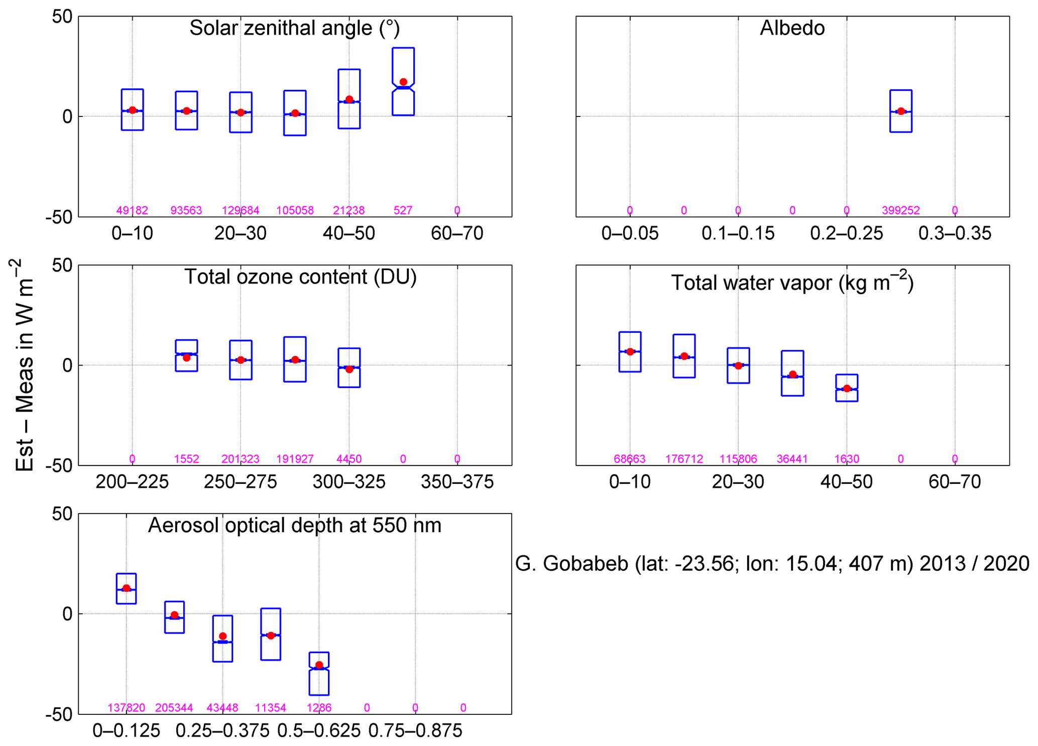
Figure 4Box plots of the differences between the McClear estimates and the measurements of G at the BSRN station Gobabeb (no. 28, climate BWh) for several classes of various variables. In each box plot, the red point is the mean while the lower, middle, and upper lines are respectively the 25th, 50th, and 75th percentiles. The number of samples is given for each class. Only classes with at least 50 samples are drawn.
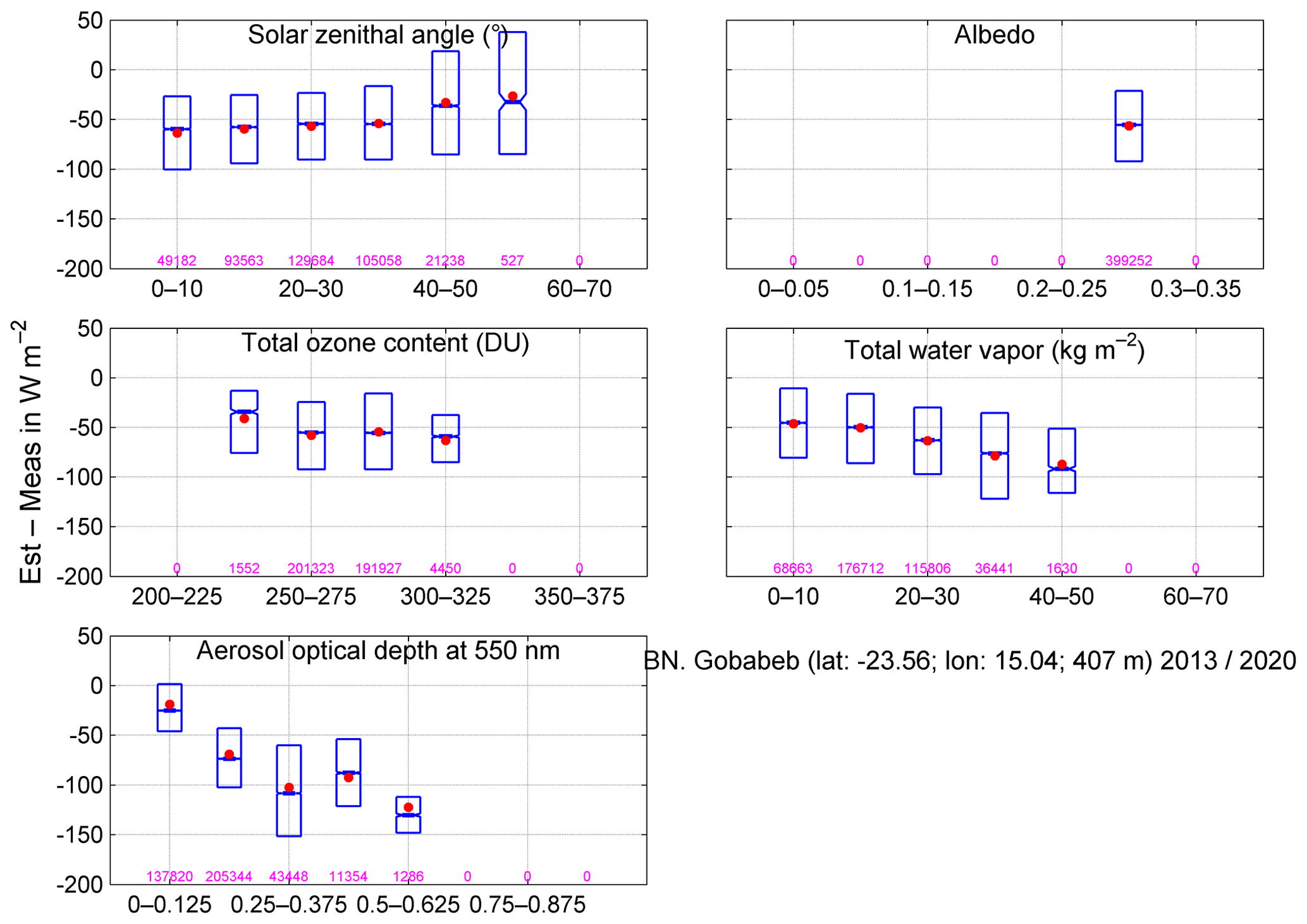
Figure 5Box plots of the differences between the McClear estimates and the measurements of BN at the BSRN station Gobabeb (no. 28, climate BWh) for several classes of various variables. In each box plot, the red point is the mean, while the lower, middle, and upper lines are respectively the 25th, 50th, and 75 percentiles. The number of samples is given for each class. Only classes with at least 50 samples are drawn.
The solar zenithal angle θS is computed with great accuracy using the SG2 algorithm and exhibits a very small uncertainty. In addition, a great deal of effort was made to accurately model the influence of θS in McClear v3, and graphs in Gschwind et al. (2019) show that the error is very small whatever θS. Hence, any error observed in box plots for θS originate from errors in other inputs, namely total column contents in ozone and water vapor, aerosol optical depth at 500 nm, and descriptors of the reflection of the ground as well as uncertainties in the McClear model. The ground albedo is a side product of McClear. It depends on the BRDF as well as on G and BN (Lefèvre et al., 2013) and includes errors on the BRDF parameters and model as well as other errors in other inputs to McClear. As such, the ground albedo is not an input to McClear and is an output of the McClear service. Nevertheless, similarly to the solar zenithal angle θS, box plots of the differences between the McClear estimates and the measurements for different classes of ground albedo have been included in Figs. 4 and 5.
As a whole, the boxes are very narrow for G (e.g., Fig. 4), which means that the intra-class variances of errors are small in contrast to BN for which boxes are much wider (e.g., Fig. 5). This is in line with the standard deviations of errors for G and BN discussed in the previous section.
The case of Gobabeb does not represent the other stations. Patterns of changes of errors with the variables depend strongly on the stations, though several rules may be found. As a whole, changes of errors with total column content in ozone or water vapor for G are small at each station (see, e.g., Fig. 4). Changes of errors are more pronounced for BN (see, e.g., Fig. 5), but there is no clear pattern as the changes depend upon the stations.
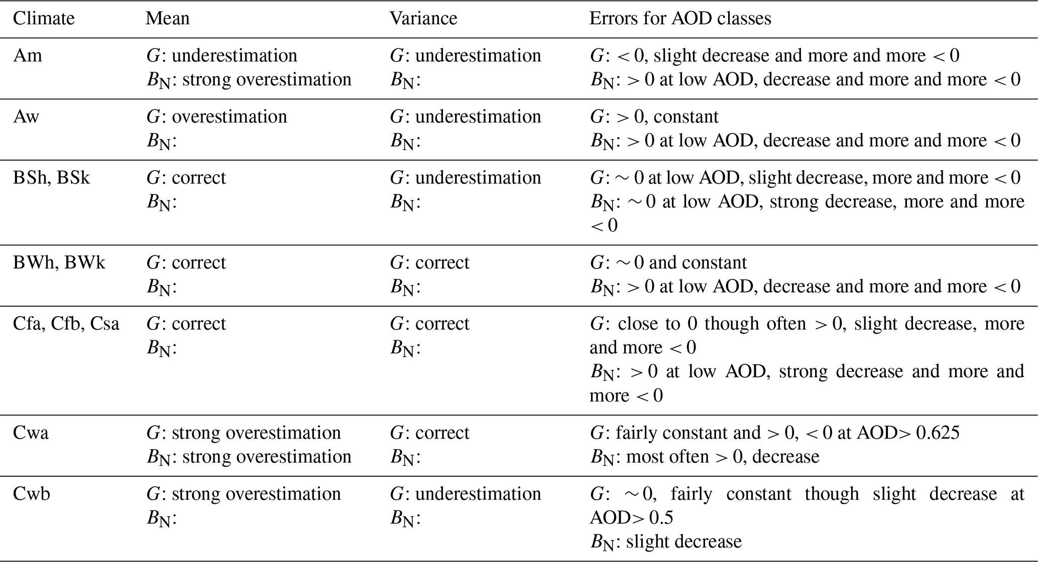
Patterns of changes of errors with aerosol optical depth (AOD) exhibit some consistency with climates, which is not the case for the total column contents in ozone and water vapor. As a whole, the errors for BN are positive or close to 0 at low AOD and decrease as the AOD increases, becoming more and more negative (see, e.g., Fig. 5). The decrease may be small (temperate climate Cwb), moderate like in Fig. 5 (tropical climates Am and Aw, desert climates BWh and BWk, temperate climate Cwa), or strong (steppe climates BSh and BSk, temperate climates Cfa, Cfb, and Csa). The patterns are more pronounced for G for each climate. Stations experiencing climate Am exhibit negative errors and a slight decrease (more and more negative) as the AOD increases, in line with the underestimation of means. The errors are positive and fairly independent of the AOD in climate Aw, in line with the overestimation of means. Errors are close to 0 and decrease slightly in climates BSh and BSk, while they are close to 0 and independent of the AOD in climates BWh (Fig. 4) and BWk and gently decreasing in climates Cfa, Cfb, and Csa; these patterns are consistent with the correct estimation of the means. In climates Cwa and Cwb, the errors are close to 0 or slightly positive and constant but slightly decrease when the AOD is greater than 0.5–0.625, in line with the overestimation of the means.
The strong dependence with AOD observed at many stations in the Supplement is quite understandable given the 1 min resolution of the measurements. The greatest CAMS AODs are likely quite rare cases of the strongest episodes that cannot be represented by pointwise 1 min measurements. One may also consider that in this kind of comparison, it is typical to see that the smallest values are overestimated and the greatest underestimated. As discussed earlier, part of the bias should be present even if both McClear and ground-based measurements were fully accurate since they do not have the same temporal and spatial scales.
Table 12 summarizes the patterns of errors with AOD for each climate and includes the errors in means and variances for both G and BN. Details are given in the Supplement. This table demonstrates clear links between climates and the errors in means and variances as well as for the AOD classes. We believe that there is no direct link between the errors in the SSI and the climates as the latter are defined from long time series of precipitation and temperature measured at stations (Peel et al., 2007). Links between climates and errors are indirect and result from combinations of shortcomings in the McClear model and gross errors in aerosol properties modeled as input to McClear, including interactions between hydrophilic species and relative humidity at each altitude and differences between the standard atmospheres used and the actual ones.
Table 12Summary of errors in means and variances and for AOD classes for each climate.
Oumbe et al. (2012a, 2013) and Eissa et al. (2015b) compared the AODs at 550 nm read from the CAMS reanalysis to AERONET measurements in the United Arab Emirates (climate BWh). They found that CAMS overestimates the AOD and that the bias increases as the AOD increases. The relative bias in AOD is in the range 10 %–20 %. These authors wrote that errors in AOD are the major source of errors in G and BN. The bias in G is negative and equal to −3 % in relative value with a relative RMSE of 5 % (Eissa et al., 2015b; Oumbe et al., 2012a). The underestimation in BN is more pronounced and is more and more negative as the AOD increases (Oumbe et al., 2012a), in agreement with our findings. Oumbe et al. (2015) underline the high variability of the bias in AOD between the stations.
Besides these above-cited early works offering detailed analyses on the United Arab Emirates and BWh climate, several articles, reports, and working papers have been published in the past few years on the comparison of CAMS AOD and AERONET measurements. Several important activities take place within the AeroCom project (https://aerocom.met.no, last access: 11 August 2022), which assembles a large number of observations and results from many global models to document and compare state-of-the-art modeling of aerosols on a global scale. The website https://aerocom-classic.met.no/cams-aerocom-evaluation/ (last access: 11 August 2022) provides interactive graphs comparing the CAMS total AOD and its components to measurements at several stations worldwide. Unfortunately, the AERONET stations available on this website do not match ours, except Hanimaadhoo (no. 5, climate Am) and Pretoria CSIR (no. 30, climate Cwb). At Hanimaadhoo, CAMS estimates are close to AERONET measurements, and one may expect small biases in G and BN, which is not the case as Tables 6 and 7 report an underestimation of −20 W m−2 for G and an overestimation of 14 W m−2 for BN. Measurements at Pretoria cover an earlier period than ours during which a strong overestimation of measurements by CAMS is observed. Particulate organic matter is the greatest contributor to the CAMS AOD. If one assumes that this overestimation also stands for the period 2018–2020, one would expect an underestimation of both G and BN, but Tables 6 and 7 indicate a slight overestimation of both. The CAMS website at https://global-evaluation.atmosphere.copernicus.eu/aerosol/aod-aeronet (last access: 27 August 2022) provides similar interactive graphs comparing the CAMS total AOD to measurements at several stations worldwide. Though this site is dedicated to the validation of the forecast 1 d ahead, it provides insight about the accuracy of CAMS AOD. There are three stations matching ours: Hanimaadhoo (no. 5, climate Am), Gobabeb (no. 28, BWh), and Durban-KZW (no. 36, Cfa), but the periods are 2020 only or 2020–2021. Comparisons with our results on the SSI may be done if one assumes that the results for AOD forecasts stand for the previous periods. At Hanimaadhoo, CAMS forecasts are close to AERONET measurements, and one may expect small biases in G and BN, which is not the case as discussed earlier about AeroCom results. Overestimations of measurements by CAMS are observed at Gobabeb and Durban. One would expect underestimations of both G and BN. Table 6 shows small positive biases for G, and Table 7 reports negative biases for BN.
Of particular interest here are the articles of Gueymard and Yang (2020) and Salamalikis et al. (2021). Both report that the AERONET AODs tend to be underestimated by CAMS in regions dominated by coarse aerosols from mineral dust and biomass burning, including our area of study. The underestimation is usually small but is highly variable in space and time. Gueymard and Yang (2020) performed a classification of the errors in AOD at 550 nm (bias and RMSE) as a function of the climate and evidenced a link between the errors and the climate, though they reported a high variability of errors within each climate (see their Figs. 6 and 9). Though there are some limitations to the direct link between errors in estimating AOD and errors in estimating G, we observe that their results may partly explain ours. In climate Am, the AOD tends to be overestimated by CAMS (see their Table 4), which is in agreement with an underestimation of G as reported in Table 12. On the contrary, the underestimation of AOD in climates Aw and Cwa (their Table 4) corresponds to an overestimation in G (Table 12). However, the relationship is not so strong. As a whole, the AOD is more or less overestimated at the AERONET stations in climates BSh, BSk, BWh, BWk, Cfa, Cfb, and Csa, while at our stations in the same climates, the estimation of G is correct (Table 12).
In this section, we have assembled the performances of McClear reported from similar previous works to assess whether our findings are in agreement with similar published works regarding the range of values for each indicator and the variability of these indicators between sites. It is also an opportunity to gather our findings and other works to establish a general overview of the performances of McClear.
Several works have been published comparing McClear outputs and in situ measurements for various summarizations. As the focus of this paper is on the assessment of performances at individual sites, we have retained in the following only those works allowing such a comparison. Results from several works cannot be compared to ours because
-
the period is very limited, such as in Dev et al. (2017), or unsuitable for comparison like the official CAMS validation reports (Lefèvre, 2021), which deal with trimesters only;
-
the work uses a special version of McClear tailored to pyranometer spectral range (Gschwind et al., 2019);
-
the work focuses on solar forecasting in all sky conditions and does not assess the performances of McClear per se (Yang, 2020); and
-
there is a lack of quantitative measures of performance at each station (Chen et al., 2020; Sun et al., 2019, 2021).
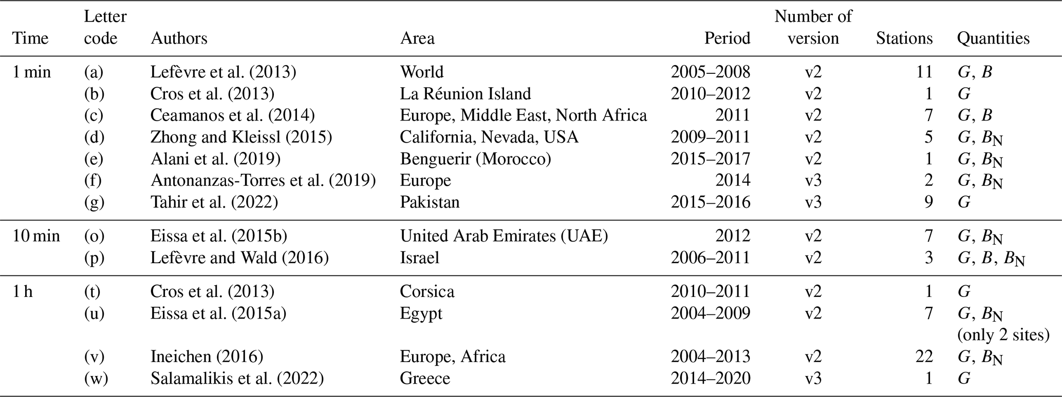
Table 13 lists the published works comparing McClear outputs and in situ measurements for summarization 1 min, 10 min, and 1 h. A letter code was assigned to each work to ease the reading of the following tables.
Table 13List of selected published works comparing McClear outputs and in situ measurements for summarization 1 min, 10 min and 1 h (column time) and some of their characteristics. The letter code is used in the following tables.
6.1 Limitations in the comparison
Comparing similar published performances with the present work is not so easy for various reasons, and some of them create limitations to the comparisons between our findings and these works and also among these works. As discussed in Sect. 2.3, the three versions, v1, v2, and v3, offer similar results and consequently the use of different versions in the selected works is not a noticeable limitation.
The use of different time periods in the compared works is a first limitation. Using sets of measurements spanning several years, Lefèvre and Wald (2016), Lefèvre et al. (2013), and Gschwind et al. (2019) observed that the statistical indicators of McClear slightly vary from one year to another for both G and B or BN, though no clear trend may be noticed. Changes in bias or standard deviations of errors of the order of 10 W m−2 for G or BN are reported by these authors, while changes in correlation coefficients are very small. These results are mostly in line with our findings in Sect. 4. Such changes with time period must be kept in mind when comparing results obtained for different years at the same station.
Another limitation is that some authors performed validation of B or D, whereas others dealt with BN. As the relationship between B and BN is not linear because of the presence of cos(θS), comparing the different results reveals difficulties. For example, the correlation coefficients for B are usually very large, whereas those for BN are smaller due to the small variances of the measurements and estimates of BN in clear-sky conditions.
The different selection of stations is a further limitation. These differences can be appreciated in the tables in the following section where we have reported all results found at individual stations by the various authors and are discussed later.
Another limitation originates from different algorithms for the selection of clear-sky instants adopted by the various authors. Table 14 lists the algorithms adopted in the works used here. To obtain a first assessment of the influence of this choice, we have compared the McClear performances found by Ceamanos et al. (2014, their Tables 6 and 4) and Lefèvre et al. (2013, their Tables 2 and 3) at the same three BSRN stations: Carpentras, Sede Boqer, and Tamanrasset. To select clear-sky instants in the measurements, Ceamanos et al. (2014) used the cloud mask provided by the NWC-SAF (http://www.nwcsaf.org/, last access: 12 August 2022), which is built and released every 15 min from infrared observations acquired aboard Meteosat satellites. This strategy provides more clear-sky instants than the algorithm of Lefèvre et al. (2013), which is more selective. Correlation coefficients are similar between the two works. The difference in bias between the two works ranges between 3 and 7 W m−2 for G and between 0 and 10 W m−2 for B. That in standard deviation of errors ranges between 4 and 10 W m−2 for G and between 3 and 35 W m−2 for B, while that in RMSE ranges between 3 and 10 W m−2 for G and between 5 and 35 W m−2 for B. Such differences may be large depending on the case. This result underlines the local influence of the algorithm for the selection of clear-sky instants and should be borne in mind when comparing published works.
Table 14List of algorithms used for detecting clear-sky instants.
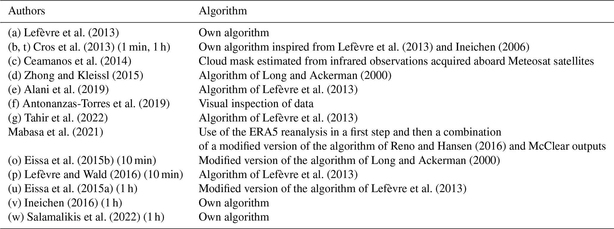
Another limitation is the summarization of the measurements, which is 1 min, 10 min, or 1 h (Table 13). Tables 15 and 16 report statistical indicators obtained at the same station for different summarizations for G and B or BN. This comparison itself has some limitations; as the selection of clear-sky instants may be different, it is limited to a small number of sites and periods of comparison are different. Having these in mind, one observes that for G, the bias has the same sign between summarizations and is often greater at 1 h than at 1 min (Table 15). The differences between 1 min and 1 h are close to those between different works at the same summarization at the same site and close to those mentioned earlier regarding different selection of clear-sky instants or different periods. The standard deviation at 1 h is less than that at 1 min, which is expected as it reflects the lower variability of the SSI and its components measured during 1 h compared to 1 min. The RMSEs are close between summarizations. There is only one station for B or BN to compare summarizations (Table 16). The correlation coefficient is less at 10 min than at 1 min, which was expected because the influence of cos(θS) on the correlation coefficient for B is less in the former case. From their own experience in validation of the SSI against ground-based measurements, the present authors have observed that, as a whole, the correlation coefficient for G and B decreases as the summarization increases from 1 min to 1 d. The bias (underestimation) is more pronounced at 10 min than at 1 min. As for BN, the statistical indicators are similar between 1 min and 1 h. The differences between statistical indicators observed at different summarizations are close to those observed between the various authors for the same summarization at the same site. Consequently, results from different summarizations may be compared with limitations similar to those reported about the algorithm for selecting clear-sky instants or different periods. However, for the sake of clarity, we have presented the statistical indicators found in the literature for each summarization in the following section.
Table 15Comparison of results obtained for G at different summarizations at the same station. N/A: not available.
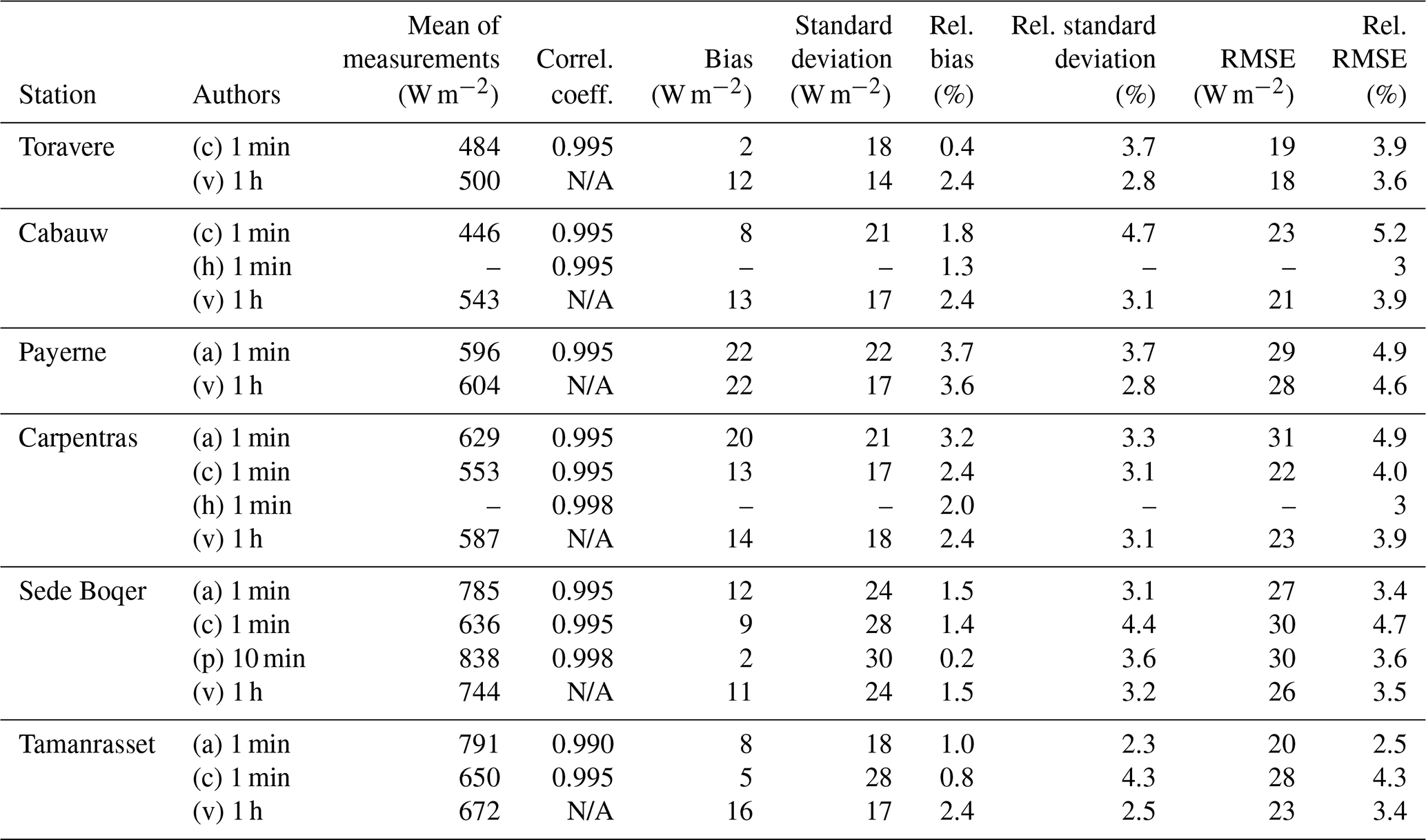
Table 16Comparison of results obtained for B or BN at different summarizations at the same station. N/A: not available.
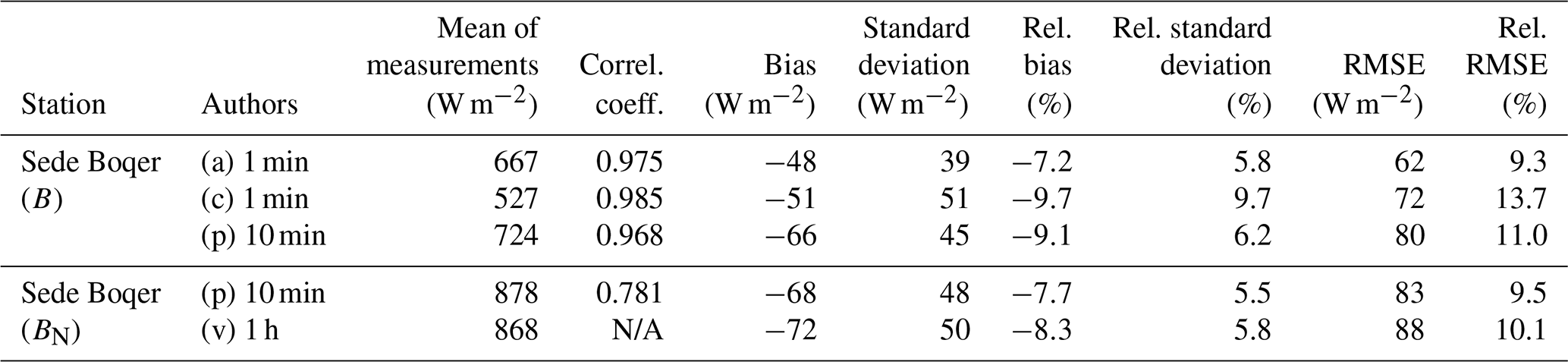
6.2 Comparison with Mabasa et al. (2021)
First of all, we have compared our results to those obtained by Mabasa et al. (2021) at 13 stations measuring G in South Africa every 1 min from 2013 to 2019. Table 17 reports the results from these authors, which are given by large intervals and may render the comparison unprecise. Only two stations in Mabasa et al. (2021) are in our list: Durban (nos. 36–37) and De Aar (no. 38). Their correlation coefficients are greater than 0.995 and greater than ours: 0.978 to 0.991. Regarding relative biases and RMSEs, ours are similar to theirs at De Aar. At Durban, our relative biases are 1.0 % and −0.2 % versus [2, 5] % for theirs, and our relative RMSEs are 2.4 % and 2.0 % versus [5, 10] % for theirs. We have also compared their results at their 13 stations (Table 17) to ours at our 16 southernmost stations from no. 27 to 44, excluding Witbank (no. 32) since the two sets of stations are located in the same region. Our correlation coefficients are between 0.966 and 0.991 and are a bit less than theirs, which are greater than 0.995. Except at three stations, their relative biases are positive and in the interval [0, 2] % at two stations and [2, 5] % at eight stations. Except at three stations, our relatives biases are positive and in the interval [0, 2] % at 10 stations and [2, 5] % at 3 stations. Our relative RMSEs lie in the interval [1.7, 4.7] %, which is a bit less than theirs: [5, 10] % in most cases. We may conclude that both studies offer similar results.
Table 17Correlation coefficient as well as biases and RMSE relative to the mean of the measurements from Mabasa et al. (2021) for G.
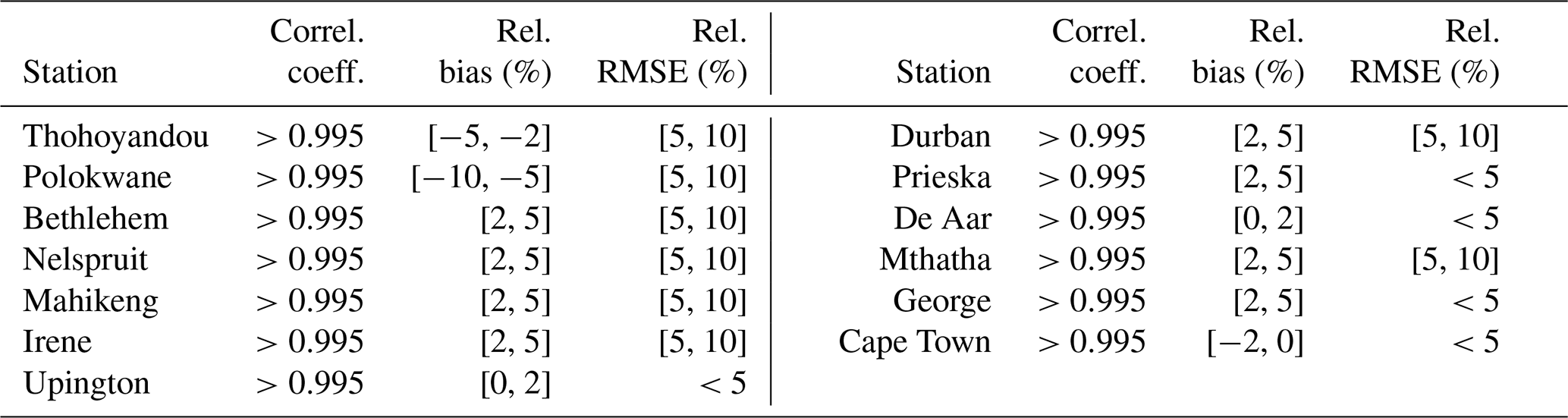
6.3 Performances reported in previous works
The results reported in other works for G and B or BN at summarizations 1 min, 10 min, and 1 h are listed in Tables B1 to B6 in Appendix B. The stations are different from ours; the objective of this section is to assess whether our findings are in agreement with similar published works regarding the range of values for each indicator and the variability of these indicators between sites. The comparison is summarized in Tables 18 (G) and 19 (B or BN). We have excluded the stations Humboldt and Sacramento, as well as all Egyptian stations but Cairo and Aswan, from our analysis for G as they exhibit extreme unexplained values compared to the other stations.
Regarding G, the correlation coefficients at 1 min (Table B1) and 10 min (Table B2) range between 0.97 and 1.00, except at Xianghe (0.954), and those at summarization 1 h (Table B3) range between 0.94 and 0.99. They are in line with ours at [0.96, 0.99] though a bit greater (Table 18). The bias is positive at most stations regardless of the summarizations, and previous results are in line with ours. The standard deviations of errors are similar between summarizations and this study (Table 18). The range of values is narrow in all cases though narrower in our study in relative value. The intervals of the RMSEs are similar between summarizations and this study (Table 18).
Looking at Table B1, we found that the mean of G is correctly estimated at stations located in climates BWh, Cfa, Cfb, and Csa, with a few exceptions in Pakistan due to local aerosol loads in dust or city pollution, and overestimated in climate Aw (Peshawar, Islamabad, Brasilia), in agreement with our own findings (see Sect. 4). The agreement is less clear at greater summarizations (Tables B2–B3).
Table 18Ranges of correlation coefficients, bias, standard deviations, RMSE, and their values relative to the mean of the measurements for G for summarizations 1 min, 10 min, and 1 h, as well as those of the present study.
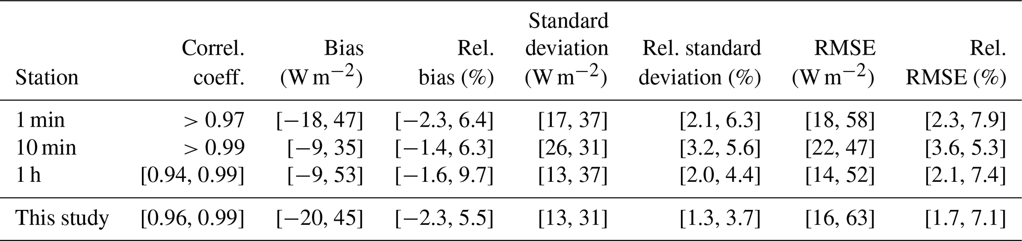
The correlation coefficients at 1 min (Table B4) for B are greater than those for BN as expected (see Sect. 6.1). The correlation coefficients at Los Angeles (Table B4) and Cairo (Table B6) are very low: 0.29 and 0.21. If we exclude the value for Los Angeles, the correlation coefficient at 1 min is in the interval [0.59, 0.94]. The intervals of the correlation coefficient are similar between summarizations and this study (Table 19). Likely because of the absence of the circumsolar radiation in the direct component in McClear, there are some slight variations between the previous works themselves and this study, especially regarding the bias. In the previous works at summarizations 1 and 10 min, the bias is most often negative (Tables B4 and B5), contrary to summarization 1 h (Table B6) and our study where more than 60 % of the stations exhibit positive biases. The ranges of relative standard deviations of errors are only fairly close between summarizations and this study (Table 19), and our study has the narrowest. The intervals of the relative RMSE are fairly similar, and this time our study has the widest interval.
Table 19Ranges of correlation coefficients, bias, standard deviations, RMSE, and their values relative to the mean of the measurements for B or BN for summarizations 1 min, 10 min, and 1 h, as well as those of the present study.
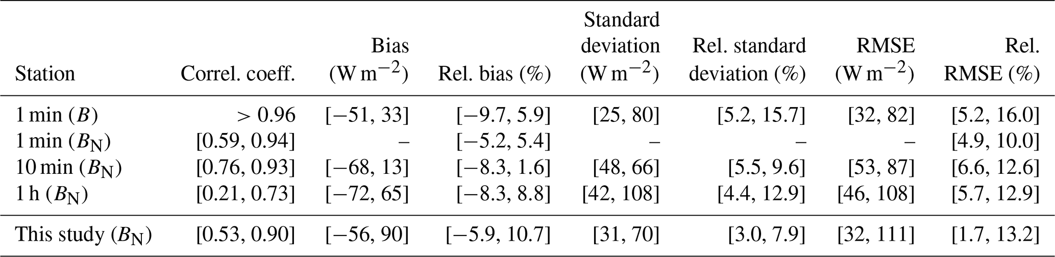
As a whole, one may conclude that our results are in agreement with those of the previous works for G and also for BN given the limitations of this comparison.
The main goal of this work was to expand and strengthen knowledge on the quality of the McClear outputs in sub-Saharan Africa and the western Indian Ocean. To this purpose, 1 min measurements from 44 stations were compared to coincident McClear outputs. The stations are located in several climates: tropical climates of monsoon (Am) and savannah (Aw) types, arid and hot or cold climates of steppe or desert types (BSh, BWh, BSk, BWk), temperate climates without a dry season and a hot or warm summer (Cfa, Cfb), temperate climates with a dry and hot summer (Csa) or dry winter and hot (Cwa) or warm (Cwb) summer. Elevations of half of the stations are greater than 100 m above sea level, up to 1914 m.
It was found that the bias for G is most often positive and ranges between −20 and 45 W m−2, i.e., between −2.3 % and 5.5 % in relative value, with a mean of 16 W m−2 (1.8 %). Half of the stations exhibit bias in the range [−15, 15] W m−2, i.e., [−1.5, 1.5] % in relative value. The variance of G is often underestimated with a ratio of variances in the interval [0.83, 1.05] with a mean of 0.95. About half of the stations (45 %) exhibit ratios between 0.95 and 1.05. The correlation coefficients between measurements and McClear estimates are greater than 0.960. The slopes of the least-squares fitting lines range between 0.88 and 1.05 and between 0.95 and 1.05 at 25 stations out of 44. The standard deviation of errors exhibits a limited range: [13, 30] W m−2, with a mean of 22 W m−2 (2.4 %). At each of the 44 stations, the relative standard deviation of errors is less than the expectations listed in Table 5: if the bias were removed, the McClear outputs would conform to the good-quality standard of the World Meteorological Organization. The RMSE lies within [17, 53] W m−2, with a mean of 31 W m−2 (3.4 %). The greater the mean clearness index at a station, the greater the correlation coefficient and the smaller the standard deviation of errors and the RMSE.
As for BN, the bias is most often positive and ranges between −48 and 62 W m−2, i.e., between −5.4 % and 7.7 % in relative value, with a mean of 11 W m−2 (1.4 %). The variance of BN is often overestimated with a ratio of variances in the interval [0.65, 1.50] with a mean of 1.07. The correlation coefficient between measurements and McClear estimates ranges between 0.532 and 0.896 and is often greater than 0.700. The slopes of the least-squares fitting lines are less than 1 and are often close to 0.80. As a whole, there is an overestimation of the smallest BN and an underestimation of the greatest ones. The standard deviation of errors is in the range [40, 69] W m−2, with a mean of 55 W m−2 (6.4 %). At each of the 44 stations, the relative standard deviation of errors is greater than the expectations listed in Table 5: if the bias were removed, the McClear outputs would not conform to the good-quality standard of the World Meteorological Organization. The RMSE lies within [42, 88] W m−2, with a mean of 63 W m−2 (7.4 %). The greater the mean clearness index at a station, the greater the correlation coefficient and the smaller the standard deviation of errors and the RMSE.
These figures for G and BN are in agreement with previously reported performances of the McClear service and therefore confirm that the performances of McClear are fairly similar worldwide as a whole. However, an in-depth analysis reveals some variability in space and time. Performances in G vary from very little from year to year at a given station. As for BN, performances from year to year at a given station vary from small to noticeable. The results show spatial consistency of performances for G and BN at short to lower mesoscales, which was one of the objectives of the inception of McClear v3 (Gschwind et al., 2019). The variability ranges from noticeable to strong at upper mesoscales and greater, except for the correlation coefficient and standard deviation of errors in G whose spatial variability is small.
This study evidences a link between the bias and ratio of variances in G and climate, which is confirmed by our analysis of the results of published works, though these findings are limited by the low number of stations and other particular conditions such as elevation. In tropical climates, the mean is underestimated in Am and overestimated in Aw, while the variance in G is underestimated. The mean is fairly correctly estimated in arid climates (BSh, BSk, BWh, BWk). The variance is underestimated in steppe (BSh, BSk) and correctly estimated in desert (BWh, BWk). The mean is fairly correctly estimated in temperate climates (Cfa, Cfb, Csa) and noticeably overestimated in climates with a dry winter: Cwa and Cwb. The variance is correctly estimated in these climates, except in Cwb due to the high elevation of the stations. Actually, the variance is underestimated at elevation greater than 1300 m whatever the climate. The influence of climate or elevation on errors in BN is much less marked than for G.
The analysis of the influence of other variables on errors suggests a major influence of the AOD. Previously published comparisons made between AERONET measurements and AOD from CAMS show links between errors in CAMS AOD and climates that may partly explain our results as well as those from similar works. Actually, the links between the climates and the errors in G and BN are indirect and result from combinations of gross errors in aerosol properties modeled in CAMS, gross errors in the exploitation of these properties in the McClear model (as discussed by Gschwind et al., 2019), and other shortcomings in the McClear model regarding reflective properties of the ground and vertical profiles of temperature, pressure, density, and volume mixing ratio for gases as a function of altitude.
This work has established an overview of the performances of the McClear service from this study and other similar published works.
It is suggested to developers of the McClear model to include in outputs of the service estimates of the SSI and its components within the spectral range of the pyranometers and its circumsolar part in order to make further comparisons between McClear outputs and measurements more accurate by (i) removing the spectral effects and (ii) easing the comparison of the direct component.
The following graphs (Figs. A1 to A5) exhibit the changes with years of the statistical quantities at each station for G and BN for the bias (Fig. A1), the relative bias (Fig. A2), the correlation coefficient (Fig. A3), the standard deviation of errors (Fig. A4), and the relative standard deviation (Fig. A5). The relative values are computed for each period and at each station by dividing by the means of the measurements for this period and this station.
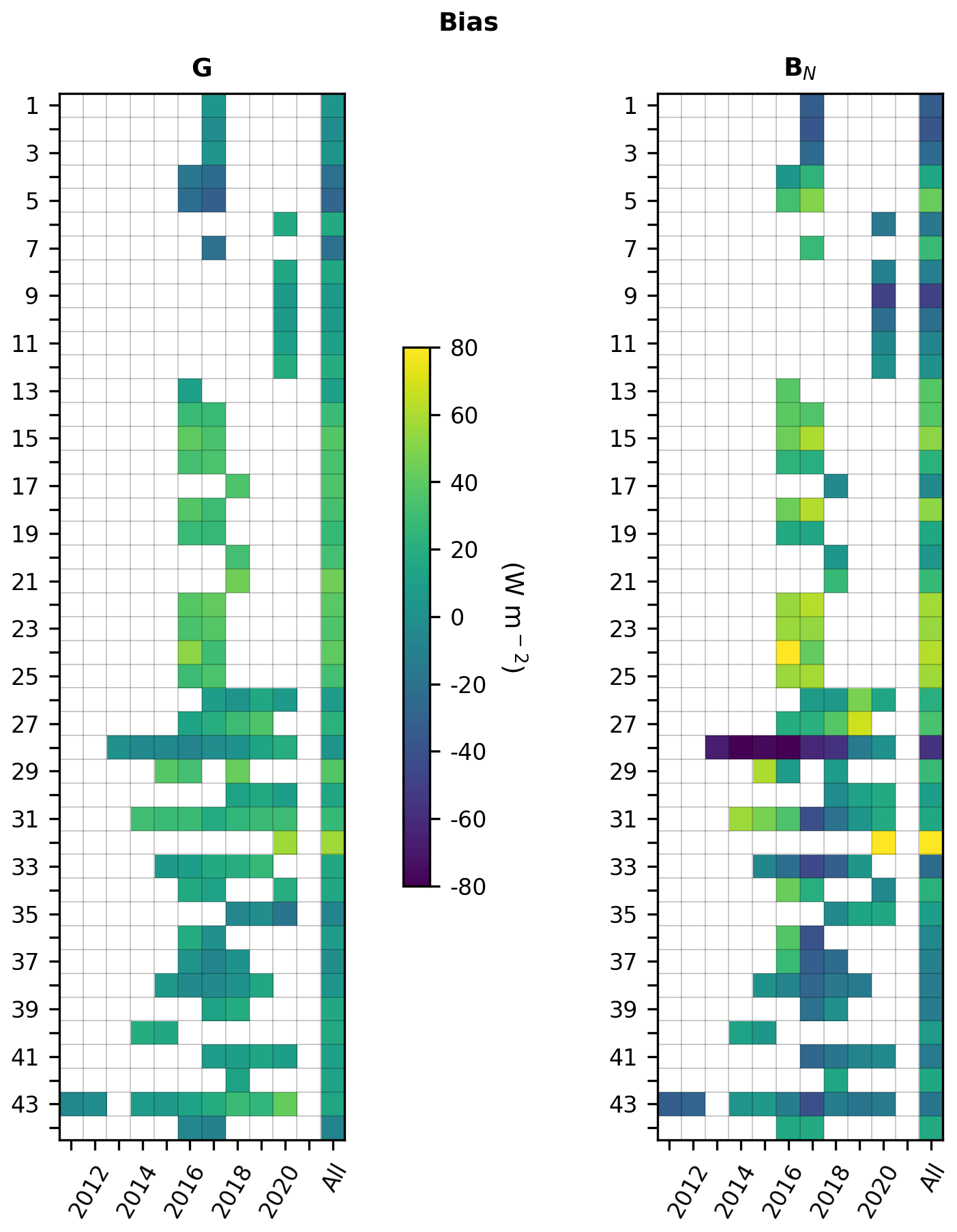
Figure A1Bias for G and BN at each station for each year and for the whole period (All). Numbers refer to the rank of the station in Table 1.
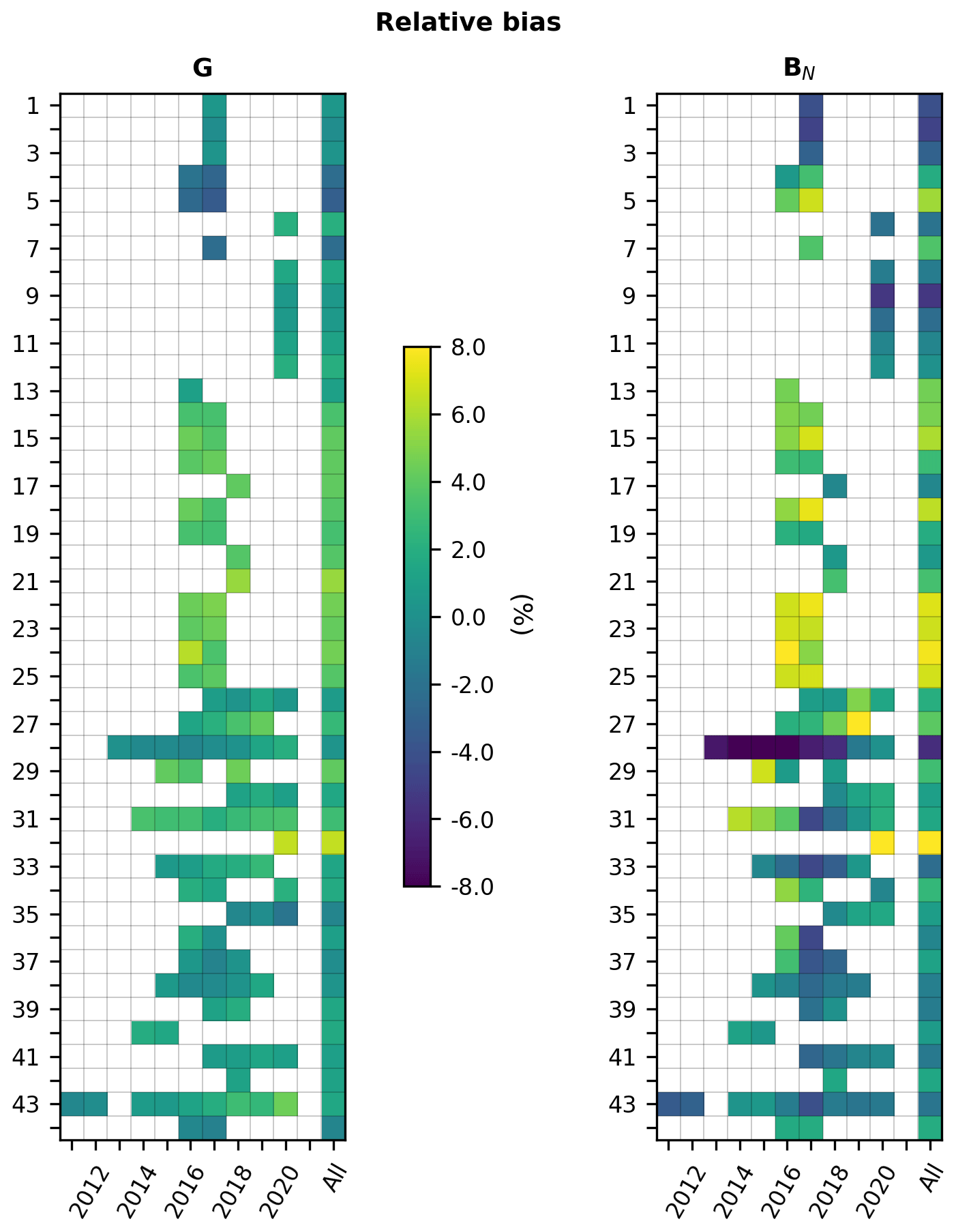
Figure A2Relative bias for G and BN at each station for each year and for the whole period (All). Numbers refer to the rank of the station in Table 1.
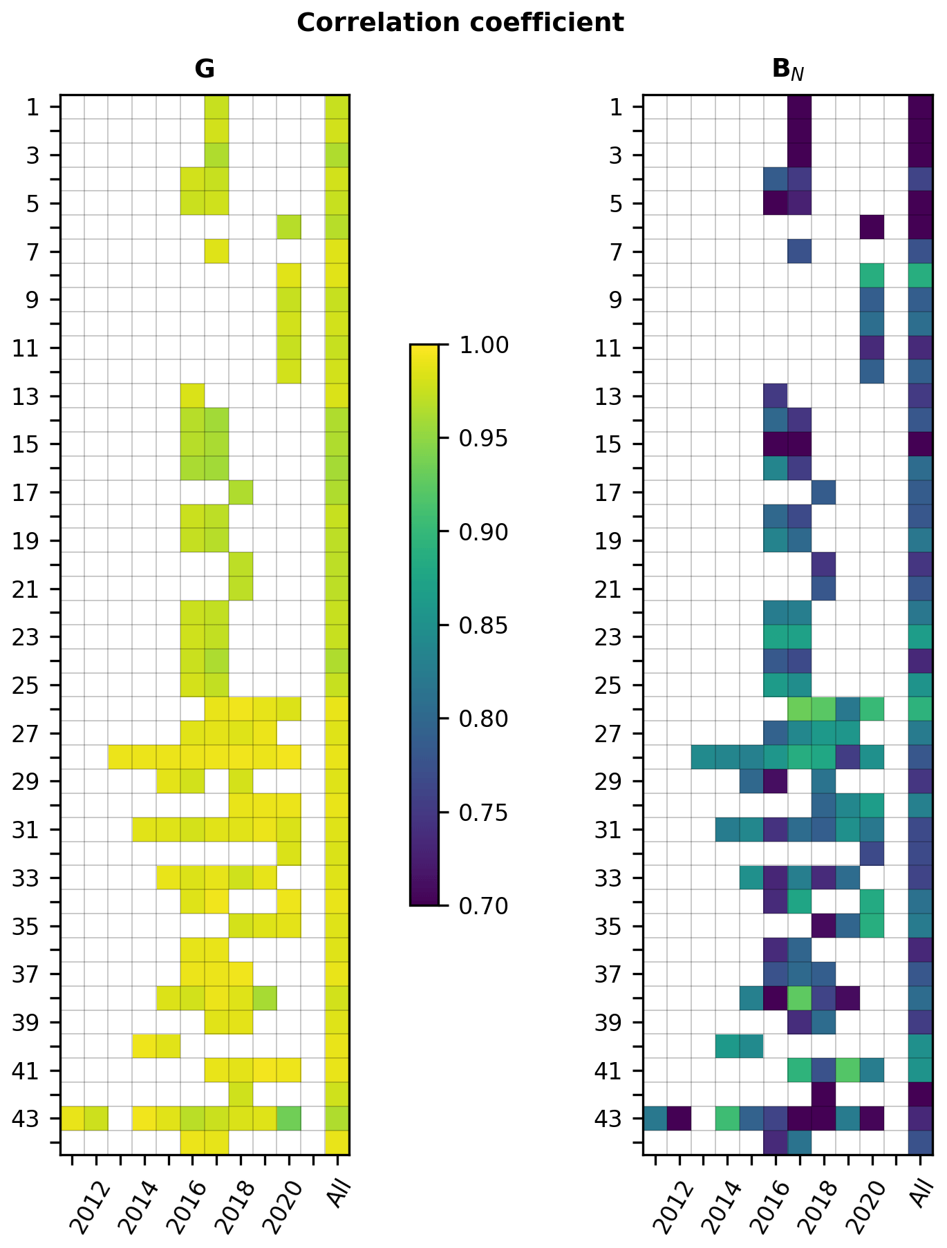
Figure A3Correlation coefficient for G and BN at each station for each year and for the whole period (All). Numbers refer to the rank of the station in Table 1.
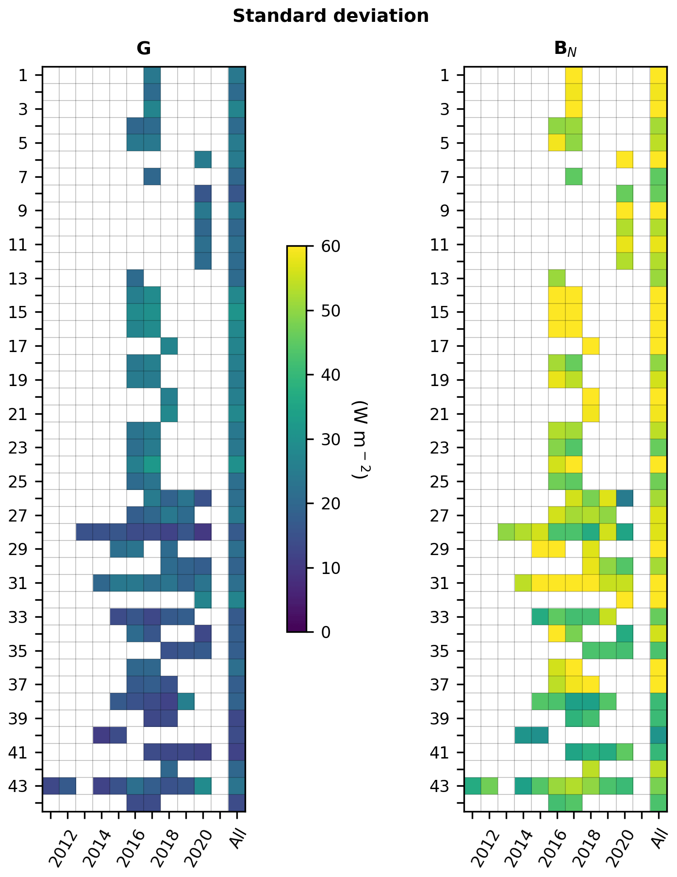
Figure A4Standard deviation of errors for G and BN at each station for each year and for the whole period (All). Numbers refer to the rank of the station in Table 1.
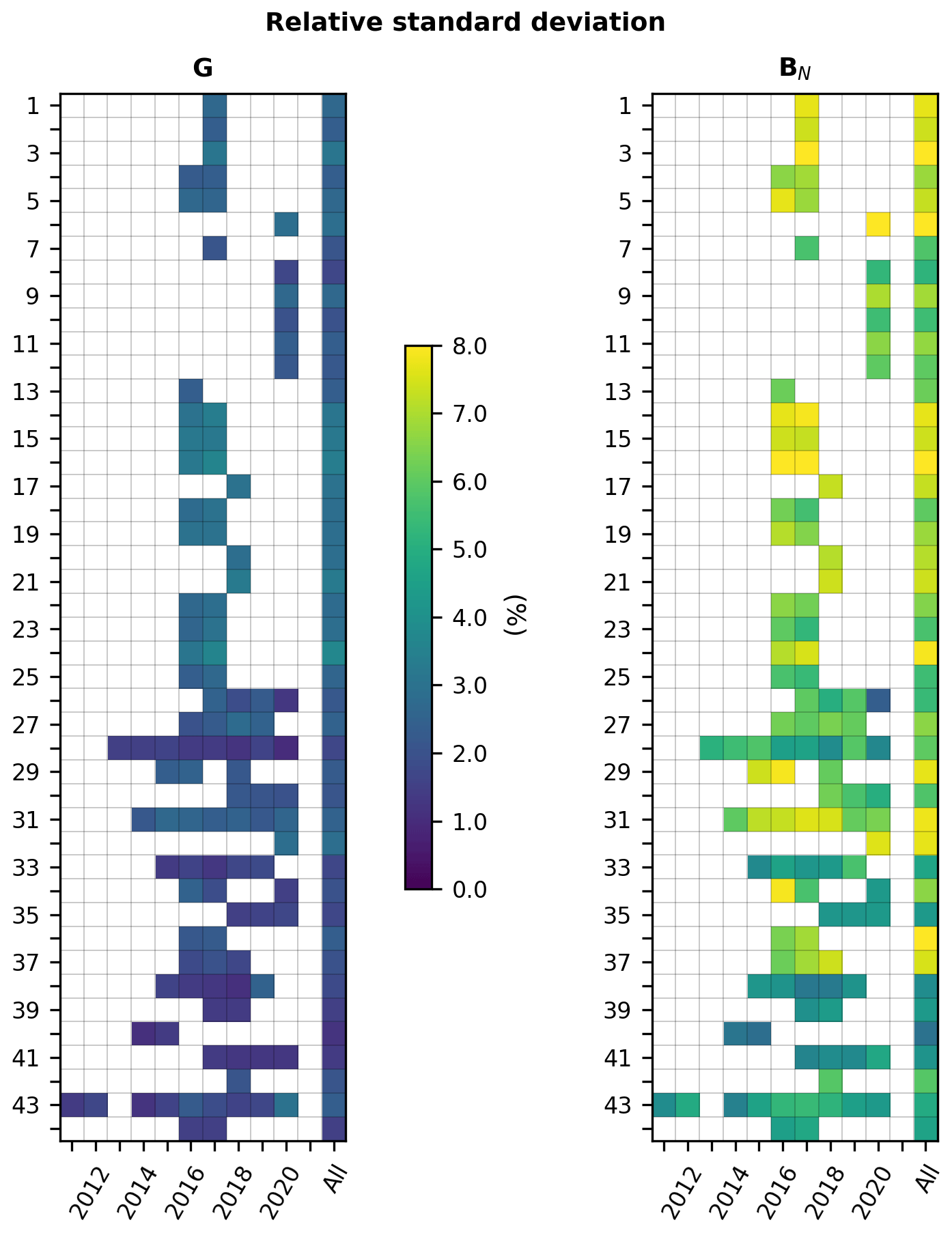
Figure A5Relative standard deviation of errors for G and BN at each station for each year and for the whole period (All). Numbers refer to the rank of the station in Table 1.
The following tables (Tables B1 to B6) list the results reported in other works for G and B or BN at summarizations 1 min, 10 min, and 1 h.
Table B1Results from previous works at summarization 1 min. Means of the measurements, correlation coefficients, bias, standard deviations, RMSE, and their values relative to the mean of the measurements for G.
Table B2Results from previous works at summarization 10 min. Means of the measurements, correlation coefficients, bias, standard deviations, RMSE, and their values relative to the mean of the measurements for G.
Table B3Results from previous works at summarization 1 h. Means of the measurements, correlation coefficients, bias, standard deviations, RMSE, and their values relative to the mean of the measurements for G.
Table B4Results from previous works at summarization 1 min. Means of the measurements, correlation coefficients, bias, standard deviations, RMSE, and their values relative to the mean of the measurements for B or BN.
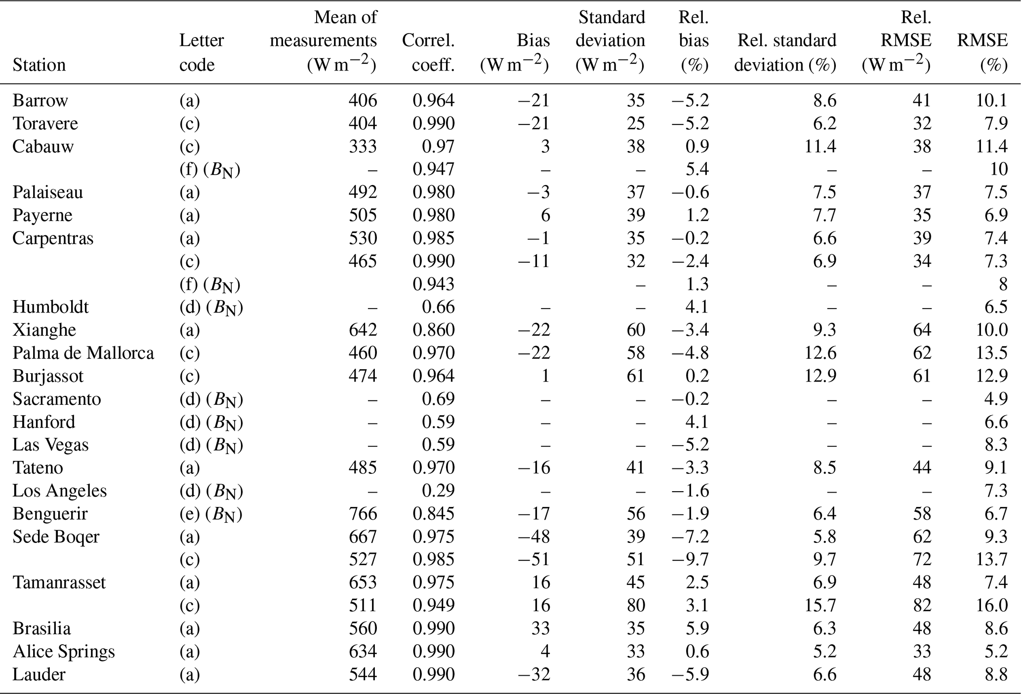
Table B5Results from previous works at summarization 10 min. Means of the measurements, correlation coefficients, bias, standard deviations, RMSE, and their values relative to the mean of the measurements for BN.
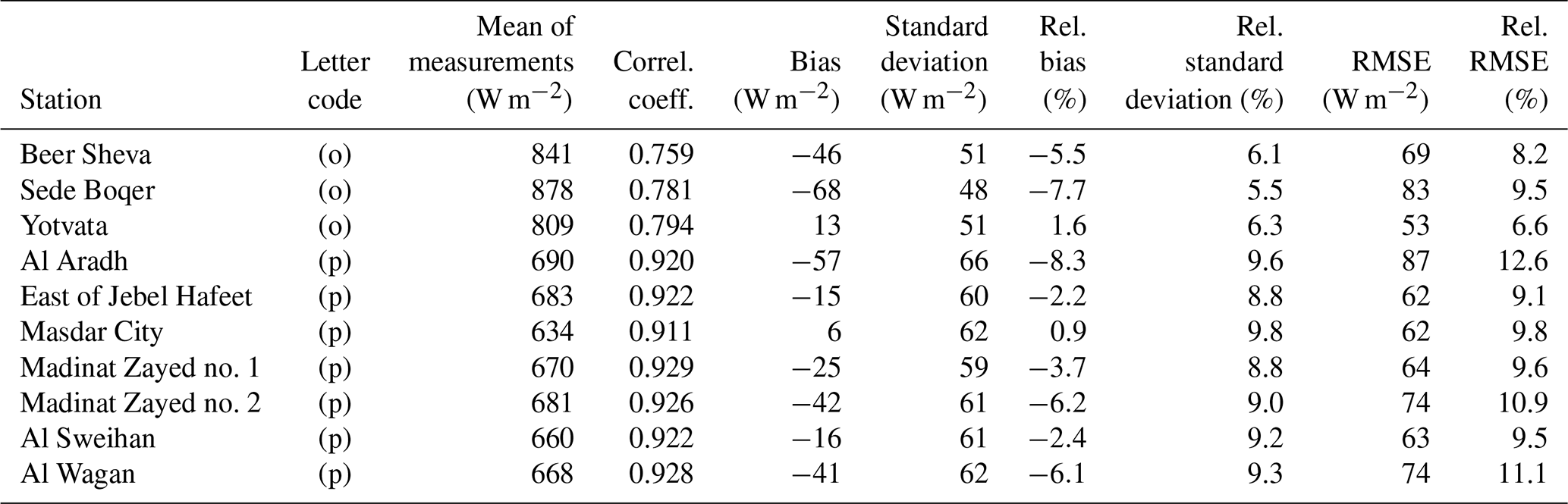
Table B6Results from previous works at summarization 1 h. Means of the measurements, correlation coefficients, bias, standard deviations, RMSE, and their values relative to the mean of the measurements for BN.
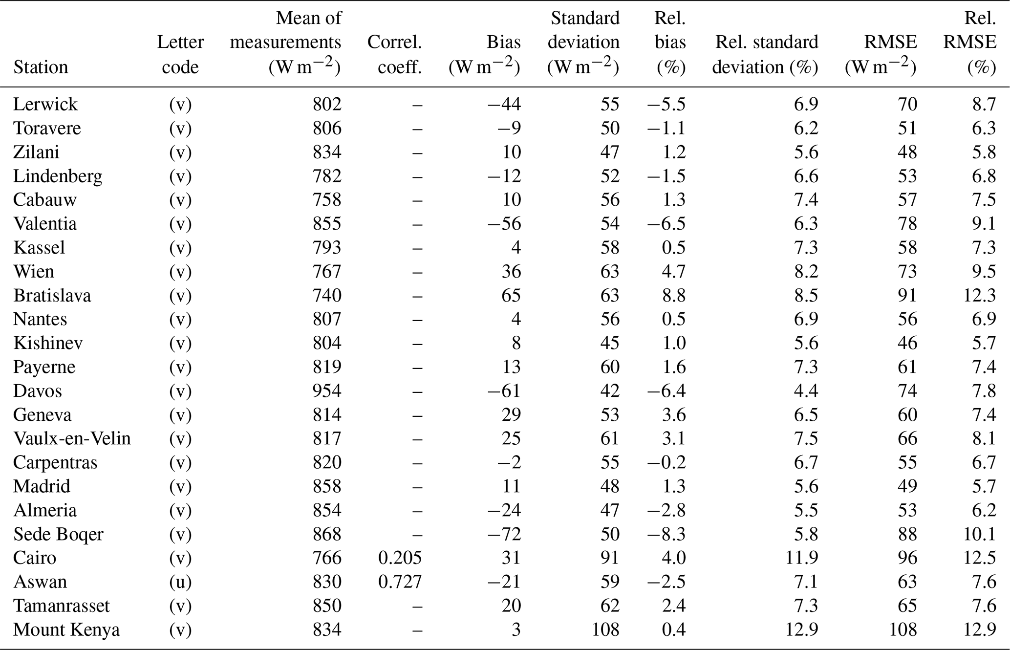
The various codes used for the comparison and plots implement well-known equations for computation of differences and statistics as well as well-known libraries in MATLAB and Python and offer no specificities.
All data used in this research can be freely accessed through several public sources. The BSRN data are the LR0100 product. They can be accessed freely upon registration at https://bsrn.awi.de (last access: 23 August 2022; Alfred-Wegener-Institute, 2022). SAURAN offers free access to its measurements via the website at https://sauran.ac.za/ (last access: 12 August 2022; Sauran, 2022). The World Bank and the International Finance Corporation, collectively the World Bank Group, have developed an open data platform – energydata.info – that provides access to a large number of datasets of solar radiation at the surface. The other measurements used in this work originate from this resource (https://energydata.info/dataset, last access: 8 August 2021; energydata, 2021). The McClear outputs and inputs from CAMS can be freely accessed upon registration at the CAMS Radiation Service (http://www.soda-pro.com/web-services/radiation/cams-mcclear, last access: 30 July 2022; ECMWF, 2022).
The supplement related to this article is available online at: https://doi.org/10.5194/amt-16-2001-2023-supplement.
The concept and design of the work were made by WWN and LW. WWN, YMSD, AA, and LW designed the methodology. WWN and YMSD identified sources of measurements from the stations, collected them, and performed their curation. WWN performed the plausibility check and the filtering of clear-sky instants. WWN collected the McClear estimates and performed the statistical analysis together with YMSD. LW did the analysis of similar previous works. All co-authors analyzed the results and contributed to the discussion. LW wrote the first draft with help from WWN and YMSD. WWN wrote the subsequent versions with contributions from all co-authors.
The contact author has declared that none of the authors has any competing interests.
Publisher's note: Copernicus Publications remains neutral with regard to jurisdictional claims in published maps and institutional affiliations.
The authors thank all operators of the ground stations whose valuable measurements they use in their work as well as the Alfred Wegener Institute, SAURAN, and the World Bank Group for hosting and maintaining the websites from which measurements can be collected.
The research leading to these results has partly received funding from the Copernicus Atmosphere Monitoring Service, a program being operated by the European Centre for Medium-Range Weather Forecasts (ECMWF) on behalf of the European Union.
This paper was edited by Udo Friess and reviewed by Brighton Mabasa and one anonymous referee.
Alani, O. E., Ghennioui, A., Merrouni, A. A., Ghennioui, H., Saint-Drenan, Y. M., and Blanc, P.: Validation of surface solar irradiances estimates and forecast under clear-sky conditions from the CAMS McClear model in Benguerir, Morocco, AIP Conference Proceedings, SolarPACES 2018, Casablanca, Morocco, October 2018, Vol. 2126, no. 1, p. 190005, https://doi.org/10.1063/1.5117702, 2019.
Alfred-Wegener-Institute: WRMC-BSRN, Alfred-Wegener-Institute [data set], https://bsrn.awi.de, last access: 23 August 2022.
Antonanzas-Torres, F., Urraca, R., Polo, J., Perpiñán-Lamigueiro, O., and Escobar, R.: Clear sky solar irradiance models: A review of seventy models, Renew. Sustain. Energy Rev., 107, 374–387, https://doi.org/10.1016/j.rser.2019.02.032, 2019.
Badosa, J., Wood, J., Blanc, P., Long, C. N., Vuilleumier, L., Demengel, D., and Haeffelin, M.: Solar irradiances measured using SPN1 radiometers: uncertainties and clues for development, Atmos. Meas. Tech., 7, 4267–4283, https://doi.org/10.5194/amt-7-4267-2014, 2014.
Bengulescu, M., Blanc, P., Boilley, A., and Wald, L.: Do modelled or satellite-based estimates of surface solar irradiance accurately describe its temporal variability?, Adv. Sci. Res., 14, 35–48, https://doi.org/10.5194/asr-14-35-2017, 2017.
Bengulescu, M., Blanc, P., and Wald, L.: On the intrinsic timescales of temporal variability in measurements of the surface solar radiation, Nonlin. Processes Geophys., 25, 19–37, https://doi.org/10.5194/npg-25-19-2018, 2018.
Blanc, P. and Wald, L.: The SG2 algorithm for a fast and accurate computation of the position of the Sun, Sol. Energy, 86, 3072–3083, https://doi.org/10.1016/j.solener.2012.07.018, 2012.
Blanc, P., Espinar, B., Geuder, N., Gueymard, C., Meyer, R., Pitz-Paal, R., Reinhardt, B., Renne, D., Sengupta, M., Wald, L., and Wilbert, S.: Direct normal irradiance related definitions and applications: the circumsolar issue, Sol. Energy, 110, 561–577, https://doi.org/10.1016/j.solener.2014.10.001, 2014a.
Blanc, P., Gschwind, B., Lefèvre, M., and Wald, L.: Twelve monthly maps of ground albedo parameters derived from MODIS data sets, Proceedings of IEEE Geoscience and Remote Sensing Symposium, held 13–18 July 2014, Quebec, Canada, 3270–3272, https://doi.org/10.1109/IGARSS.2014.6947177, 2014b.
Bojinski, S., Verstraete, M., Peterson, T. C., Richter, C., Simmons, A., and Zemp, M.: The concept of essential climate variables in support of climate research, applications, and policy, B. Am. Meteorol. Soc., 95, 1431–1443, https://doi.org/10.1175/BAMS-D-13-00047.1, 2014.
Bright, J. M., Sun, X., Gueymard, C. A., Acord, B., Wang, P., and Engerer, N. A.: Bright-Sun. A globally applicable 1-min irradiance clear-sky detection model, Renew. Sustain. Energy Rev., 121, 09706, https://doi.org/10.1016/j.rser.2020.109706, 2020.
Brooks, M. J., du Clou, S., van Niekerk, W. L., Gauché, P., Leonard, C., Mouzouris, M. J., Meyer, R., van der Westhuizen, N., van Dyk, E. E, and Vorster, F. J.: SAURAN: A new resource for solar radiometric data in Southern Africa, Journal of Energy in Southern Africa, 26, 2–10, http://www.scielo.org.za/scielo.php?script=sci_arttext&pid=S1021-447X2015000100001&lng=en&tlng=en (last access: 30 October 2021), 2015.
Calbó, J., González, J. A., and Pagès, D.: A method for sky-condition classification from ground-based solar radiation measurements, J. Appl. Meteorol., 40, 2193–2199, https://doi.org/10.1175/1520-0450(2001)040<2193:AMFSCC>2.0.CO;2, 2001.
Ceamanos, X., Carrer, D., and Roujean, J.-L.: Improved retrieval of direct and diffuse downwelling surface shortwave flux in cloudless atmosphere using dynamic estimates of aerosol content and type: application to the LSA-SAF project, Atmos. Chem. Phys., 14, 8209–8232, https://doi.org/10.5194/acp-14-8209-2014, 2014.
Chen, X. M., Li, Y., and Wanga, R. Z.: Performance study of affine transformation and the advanced clear-sky model to improve intra-day solar forecasts, J. Renew. Sustain. Ener., 12, 043703, https://doi.org/10.1063/5.0009155, 2020.
Cros, S., Liandrat, O., Sébastien, N., Schmutz, N., and Voyant, C.: Clear sky models assessment for an operational PV production forecasting solution, 28th European Photovoltaic Solar Energy Conference and Exhibition, Sep 2013, France, 5BV.4.69, 2013, https://www.eupvsec-proceedings.com/proceedings?paper=26738, last access: 14 July 2021.
Dantas de Paula, M., Gómez Giménez, M., Niamir, A., Thurner, M., and Hickler, T.: Combining European earth observation products with dynamic global vegetation models for estimating essential biodiversity variables, Int. J. Digit. Earth, 13, 262–277, https://doi.org/10.1080/17538947.2019.1597187, 2020.
Dev, S., Manandhar, S., Lee, Y. H., and Winkler, S.: Study of clear sky models for Singapore, 38th Progress in Electromagnetics Research Symposium (PIERS), 22–25 May 2017, https://ieeexplore.ieee.org/document/8293352/, last access: 15 July 2021.
ECMWF: CAMS McClear Service for irradiation under clear-sky, Atmosphere Monitoring Service [data set], http://www.soda-pro.com/web-services/radiation/cams-mcclear, last access: 30 July 2022.
Eissa, Y., Korany, M., Aoun, Y., Boraiy, M., Abdel Wahab, M., Alfaro, S., Blanc, P., El-Metwally, M., Ghedira, H., and Wald, L.: Validation of the surface downwelling solar irradiance estimates of the HelioClim-3 database in Egypt, Remote Sens-Basel, 7, 9269–9291, https://doi.org/10.3390/rs70709269, 2015a.
Eissa, Y., Munawwar, S., Oumbe, A., Blanc, P., Ghedira, H., Wald, L., Bru, H., and Goffe, D.: Validating surface downwelling solar irradiances estimated by the McClear model under cloud-free skies in the United Arab Emirates, Sol. Energy, 114, 17–31, https://doi.org/10.1016/j.solener.2015.01.017, 2015b.
Eissa, Y., Blanc, P., Ghedira, H., Oumbe, A., and Wald, L.: A fast and simple model to estimate the contribution of the circumsolar irradiance to measured broadband beam irradiance under cloud-free conditions in desert environment, Sol. Energy, 163, 497–509, https://doi.org/10.1016/j.solener.2018.02.015, 2018.
Ellis, B. H, Deceglie, M., and Jain, A.: Automatic detection of clear-sky periods from irradiance data, IEEE J. Photovoltaics, 9, 998–1005, https://doi.org/10.1109/JPHOTOV.2019.2914444, 2019.
Emde, C., Buras-Schnell, R., Kylling, A., Mayer, B., Gasteiger, J., Hamann, U., Kylling, J., Richter, B., Pause, C., Dowling, T., and Bugliaro, L.: The libRadtran software package for radiative transfer calculations (version 2.0.1), Geosci. Model Dev., 9, 1647–1672, https://doi.org/10.5194/gmd-9-1647-2016, 2016.
energydata: 970 datasets, energydata [data set], https://energydata.info/dataset, last access: 8 August 2021.
Fountoulakis, I., Papachristopoulou, K., Proestakis, E., Amiridis, V., Kontoes, C., and Kazadzis, S.: Effect of aerosol vertical distribution on the modeling of solar radiation, Remote Sens.-Basel, 14, 1143, https://doi.org/10.3390/rs14051143, 2022.
GEO (Group on Earth Observations): GEO Task US-09-01a: Critical Earth Observations Priorities. Health Societal Benefit Area: Air Quality, https://sbageotask.larc.nasa.gov/AirQuality_US0901a-FINAL.pdf (last access: 11 July 2022), 2010.
GEO (Group on Earth Observations): The GEOSS Water Strategy: From Observations to Decisions, https://www.ceos.org/document_management/Ad_Hoc_Teams/WSIST/WSIST_GEOSS-Water-Strategy-Full-Report_Jan2014.pdf (last access: 12 July 2021), 2014.
Gschwind, B., Ménard, L., Albuisson, M., and Wald, L.: Converting a successful research project into a sustainable service: the case of the SoDa Web service, Environ. Modell. Softw., 21, 1555–1561, https://doi.org/10.1016/j.envsoft.2006.05.002, 2006.
Gschwind, B., Wald, L., Blanc, P., Lefèvre, M., Schroedter-Homscheidt, M., and Arola, A.: Improving the McClear model estimating the downwelling solar radiation at ground level in cloud-free conditions – McClear-v3, Meteorol. Z., 28, 147–163, https://doi.org/10.1127/metz/2019/0946, 2019.
Gueymard, C. A.: Spectral circumsolar radiation contribution to CPV, AIP Conference Proceedings 1277, 6th International Conference on Concentrating Photovoltaic Systems, Freiburg, Germany, 7–9 April 2010, 316, https://doi.org/10.1063/1.3509220, 2010.
Gueymard, C. A.: Clear-sky irradiance predictions for solar resource mapping and large-scale applications: Improved validation methodology and detailed performance analysis of 18 broadband radiative models, Sol. Energy, 86, 2145–2169, https://doi.org/10.1016/j.solener.2011.11.011, 2012.
Gueymard, C. A. and Yang, D.: Worldwide validation of CAMS and MERRA-2 reanalysis aerosol optical depth products using 15 years of AERONET observations, Atmos. Environ., 225, 117216, https://doi.org/10.1016/j.atmosenv.2019.117216, 2020.
Ineichen, P.: Comparison of eight clear sky broadband models against 16 independent data banks, Sol. Energy, 80, 468–478, https://doi.org/10.1016/j.solener.2005.04.018, 2006.
Ineichen, P.: Validation of models that estimate the clear sky global and beam solar irradiance, Sol. Energy, 132, 332–344, https://doi.org/10.1016/j.solener.2016.03.017, 2016.
Juzeniene, A., Brekke, P., Dahlback, A., Andersson-Engels, S., Reichrath, J., Moan, K., Holick, M. F., Grant, W. B., and Moan, J.: Solar radiation and human health, Rep. Prog. Phys., 74, 066701, https://doi.org/10.1088/0034-4885/74/6/066701, 2011.
Kasten, F. and Young, A. T.: Revised optical air mass tables and approximation formula, Appl. Opt., 28, 4735–4738, https://doi.org/10.1364/AO.28.004735, 1989.
Kato, S., Ackerman, T., Mather, J., and Clothiaux, E.: The k–distribution method and correlated–k approximation for shortwave radiative transfer model, J. Quant. Spectrosc. Ra., 62, 109–121, https://doi.org/10.1016/S0022-4073(98)00075-2, 1999.
Kopp, G. and Lean, J. L.: A new, lower value of total solar irradiance: evidence and climate significance, Geophys. Res. Lett., 38, L01706, https://doi.org/10.1029/2010GL045777, 2011.
Korany, M., Boraiy, M., Eissa, Y., Aoun, Y., Abdel Wahab, M. M., Alfaro, S. C., Blanc, P., El-Metwally, M., Ghedira, H., Hungershoefer, K., and Wald, L.: A database of multi-year (2004–2010) quality-assured surface solar hourly irradiation measurements for the Egyptian territory, Earth Syst. Sci. Data, 8, 105–113, https://doi.org/10.5194/essd-8-105-2016, 2016.
Lean, J. and Rind, D.: Climate forcing by changing solar radiation, J. Climate, 11, 3069–3094, 1998.
Lefèvre, M.: Regular validation reports of the CAMS solar radiation products. Issues #33 and 34, https://atmosphere.copernicus.eu/supplementary-services (last access: 30 August 2022), 2021.
Lefèvre, M. and Wald, L.: Validation of the McClear clear-sky model in desert conditions with three stations in Israel, Adv. Sci. Res., 13, 21–26, https://doi.org/10.5194/asr-13-21-2016, 2016.
Lefèvre, M., Blanc, P., Espinar, B., Gschwind, B., Ménard, L., Ranchin, T., Wald, L., Saboret, L., Thomas, C., and Wey, E.: The HelioClim-1 database of daily solar radiation at Earth surface: an example of the benefits of GEOSS Data-CORE, IEEE J. Select. Top. Appl. Earth Observ. Remote Sens., 7, 1745–1753, https://doi.org/10.1109/JSTARS.2013.2283791, 2014.
Lefèvre, M., Oumbe, A., Blanc, P., Espinar, B., Gschwind, B., Qu, Z., Wald, L., Schroedter-Homscheidt, M., Hoyer-Klick, C., Arola, A., Benedetti, A., Kaiser, J. W., and Morcrette, J.-J.: McClear: a new model estimating downwelling solar radiation at ground level in clear-sky conditions, Atmos. Meas. Tech., 6, 2403–2418, https://doi.org/10.5194/amt-6-2403-2013, 2013.
Long, C. N. and Ackerman, T. P.: Identification of clear skies from broadband pyranometer measurements and calculation of downwelling shortwave cloud effects, J. Geophys. Res., 105, 15609, https://doi.org/10.1029/2000JD900077, 2000.
Mabasa, B., Lysko, M. D., Tazvinga, H., Zwane, N., and Moloi, S. J.: The performance assessment of six global horizontal irradiance clear sky models in six climatological regions in South Africa, Energies, 14, 2583, https://doi.org/10.3390/en14092583, 2021.
Mayer, B. and Kylling, A.: Technical note: The libRadtran software package for radiative transfer calculations - description and examples of use, Atmos. Chem. Phys., 5, 1855–1877, https://doi.org/10.5194/acp-5-1855-2005, 2005.
Möllenkamp, J., Beikircher, T., and Häberle, A.: Recalibration of SPN1 pyranometers against pyrheliometer and its relevance for the evaluation of concentrating solar process heat plants, Sol. Energy, 197, 344–358, https://doi.org/10.1016/j.solener.2019.12.055, 2020.
Ohmura, A., Gilgen, H., Hegner, H., Mueller, G., Wild, M., Dutton, E. G., Forgan, B., Froelich, C., Philipona, R., Heimo, A., Koenig-Langlo, G., McArthur, B., Pinker, R., Whitlock, C. H., and Dehne, K.: Baseline Surface Radiation Network (BSRN/WCRP): New precision radiometry for climate research, B. Am. Meteorol. Soc., 79, 2115–2136, https://doi.org/10.1175/1520-0477(1998)079<2115:BSRNBW>2.0.CO;2, 1998.
Oumbe, A., Wald, L., Blanc, P., and Schroedter-Homscheidt, M.: Exploitation of radiative transfer model for assessing solar radiation: the relative importance of atmospheric constituents, EUROSUN 2008, 1st International Congress on Heating, Cooling and Buildings, Lisbon, Portugal, Oct 2008, Paper 403, https://hal-mines-paristech.archives-ouvertes.fr/hal-00465779 (last access: 19 June 2022), 2008.
Oumbe, A., Bru, H., Hassar, Z., Blanc, P., Wald, L., Fournier, A., Goffe, D., Chiesa, M., and Ghedira, H.: Selection and implementation of aerosol data for the prediction of solar resource in United Arab Emirates, SolarPaces Symposium, held in Marrakech, Morocco, on 11–14 September 2012, USBKey Paper#22240, https://hal-mines-paristech.archives-ouvertes.fr/hal-00779749 (last access: 26 July 2022), 2012a.
Oumbe, A., Qu, Z., Blanc, P., Bru, H., Lefèvre, M., and Wald, L.: Modeling circumsolar irradiance to adjust beam irradiances from radiative transfer models to measurements, EMS Annual Meeting 2012, Lodz, Poland, 10–14 September 2012, EMS2012-152, https://meetingorganizer.copernicus.org/EMS2012/EMS2012-152.pdf (last access: 2 October 2021), 2012b.
Oumbe, A., Bru, H., Hassar, Z., Blanc, P., Wald, L., Eissa, Y., Marpu, P., Gherboudj, I., Ghedira, H., and Goffe, D.: On the improvement of MACC aerosol spatial resolution for irradiance estimation in the United Arab Emirates, 2013 ISES Solar World Congress, held in Cancun, Mexico, 3–7 November 2013, https://hal.archives-ouvertes.fr/hal-01493638 (last access: 265 July 2022), 2013.
Oumbe, A., Qu, Z., Blanc, P., Lefèvre, M., Wald, L., and Cros, S.: Decoupling the effects of clear atmosphere and clouds to simplify calculations of the broadband solar irradiance at ground level, Geosci. Model Dev., 7, 1661–1669, https://doi.org/10.5194/gmd-7-1661-2014, 2014.
Peel, M. C., Finlayson, B. L., and McMahon, T. A.: Updated world map of the Köppen-Geiger climate classification, Hydrol. Earth Syst. Sci., 11, 1633–1644, https://doi.org/10.5194/hess-11-1633-2007, 2007.
Perez, R., Ineichen, P., Seals, R. and Zelenka, A.: Making full use of the clearness index for parameterizing hourly insolation conditions, Sol. Energy, 45, 111–114, https://doi.org/10.1016/0038-092X(90)90036-C, 1990.
Perez, R., Seals, R., and Zelenka, A.: Comparing satellite remote sensing and ground network measurements for the production of site/time specific irradiance data, Sol. Energy, 60, 89–96, https://doi.org/10.1016/S0038-092X(96)00162-4, 1997.
Qin, Y., McVicar, T. R., Huang, J., West, S., and Steven, A. D. L.: On the validity of using ground-based observations to validate geostationary-satellite-derived direct and diffuse surface solar irradiance: Quantifying the spatial mismatch and temporal averaging issues, Remote Sens. Environ., 280, 113179, https://doi.org/10.1016/j.rse.2022.113179, 2022.
Qu, Z., Oumbe, A., Blanc, P., Espinar, B., Gesell, G., Gschwind, B., Klüser, L., Lefèvre, M., Saboret, L., Schroedter-Homscheidt, M., and Wald L.: Fast radiative transfer parameterisation for assessing the surface solar irradiance: The Heliosat-4 method, Meteorol. Z., 26, 33–57, https://doi.org/10.1127/metz/2016/0781, 2017.
Ranchin, T., Trolliet, M., Ménard, L., and Wald, L.: Which variables are essential for renewable energies?, Int. J. Digit. Earth, 13, 253–261, https://doi.org/10.1080/17538947.2019.1679267, 2020.
Reno, M. J. and Hansen, C. W.: Identification of periods of clear sky irradiance in time series of GHI measurements, Renew. Energ., 90, 520–531, https://doi.org/10.1016/j.renene.2015.12.031, 2016.
Rigollier, C., Bauer, O., and Wald, L.: On the clear sky model of the ESRA – European Solar Radiation Atlas with respect to the Heliosat method, Sol. Energy, 68, 33–48, https://doi.org/10.1016/S0038-092X(99)00055-9, 2000.
Roesch, A., Wild, M., Ohmura, A., Dutton, E. G., Long, C. N., and Zhang, T.: Assessment of BSRN radiation records for the computation of monthly means, Atmos. Meas. Tech., 4, 339–354, https://doi.org/10.5194/amt-4-339-2011, 2011.
Salamalikis, V., Tzoumanikas, P., Argiriou, A. A., and Kazantzidis, A.: Site adaptation of global horizontal irradiance from the Copernicus Atmospheric Monitoring Service for radiation using supervised machine learning techniques, Renew. Energ., 195, 92–106, https://doi.org/10.1016/j.renene.2022.06.043, 2022.
Salamalikis, V., Vamvakas, I., Blanc, P., and Kazantzidis, A.: Ground-based validation of aerosol optical depth from CAMS reanalysis project: An uncertainty input on direct normal irradiance under cloud-free conditions, Renew. Energ., 170, 847–857, https://doi.org/10.1016/j.renene.2021.02.025, 2021.
Sauran: Southern African Universities Radiometric Network, Sauran [data set], https://sauran.ac.za/, last access: 12 August 2022.
Schaaf, C. B., Gao, F., Strahler, A. H., Lucht, W., Li, X. W., Tsang, T., Strugnell, N. C., Zhang, X. Y., Jin, Y. F., Muller, J. P., Lewis, P., Barnsley, M., Hobson, P., Disney, M., Roberts, G., Dunderdale, M., Doll, C., d'Entremont, R. P., Hu, B. X., Liang, S. L., Privette, J. L., and Roy, D.: First operational BRDF, albedo nadir reflectance products from MODIS, Remote Sens. Environ., 83, 135–148, https://doi.org/10.1016/S0034-4257(02)00091-3, 2002.
Schroedter-Homscheidt, M.: The Copernicus Atmosphere Monitoring Service (CAMS) Radiation Service in a nutshell, v11, https://atmosphere.copernicus.eu/sites/default/files/2020-03/Copernicus_radiation_service_in_nutshell_v11.pdf (last access: 2 October 2021), 2019.
Sengupta, M., Habte, A., Wilbert, A., Gueymard, C., and Remund, J.: Best Practices Handbook for the Collection and Use of Solar Resource Data for Solar Energy Applications, 3rd Edn., Golden, Colorado, USA, National Renewable Energy Laboratory, NREL/TP-5D00-77635, https://www.nrel.gov/docs/fy21osti/77635.pdf, last access: 5 August 2021.
Sun, X., Bright, J. M., Gueymard, C. A., Acord, B., Wang, P., and Engerer, N. A.: Worldwide performance assessment of 75 global clear-sky irradiance models using principal component analysis, Renew. Sustain. Energy Rev., 111, 550–570, https://doi.org/10.1016/j.rser.2019.04.006, 2019.
Sun, X., Bright, J. M., Gueymard, C. A., Bai, X., Acord, B., and Wang, P.: Worldwide performance assessment of 95 direct and diffuse clear-sky irradiance models using principal component analysis, Renew. Sustain. Energy Rev., 135, 110087, https://doi.org/10.1016/j.rser.2020.110087, 2021.
Sun, X., Yang, D., Gueymard, C. A., Bright, J. M., and Wang, P.: Effects of spatial scale of atmospheric reanalysis data on clear-sky surface radiation modeling in tropical climates: A case study for Singapore, Sol. Energy, 525–537, https://doi.org/10.1016/j.solener.2022.06.001, 2022.
Tahir, Z. R., Amjad, G. M., Hamza, M., Shad, M. R., Qamar, A., Blanc, P., Abbas, S., Azhar, M., Safyan, M., Abdullah, M., Atif, M., and Haider, S. T.: Validating global horizontal irradiance estimated by McClear model under clear-sky and all-sky conditions in Pakistan, Energ. Environ.-UK, https://doi.org/10.1177/0958305X221118869, 2022.
Vuilleumier, L., Hauser, M., Félix, C., Vignola, F., Blanc, P., Kazantzidis, A., and Calpini, B.: Accuracy of ground surface broadband shortwave radiation monitoring, J. Geophys. Res.-Atmos., 119, 13838–13860, https://doi.org/10.1002/2014JD022335, 2014.
Wald, L.: Fundamentals of Solar Radiation, CRC Press, London, United Kingdom, 270 pp., https://doi.org/10.1201/9781003155454, 2021.
Wald, L. and Baleynaud, J.-M.: Observing air quality over the city of Nantes by means of Landsat thermal infrared data, Int. J. Remote Sens., 20, 947–959, https://doi.org/10.1080/014311699213019, 1999.
Wandji Nyamsi, W., Espinar, B., Blanc, P., and Wald, L.: How close to detailed spectral calculations is the k-distribution method and correlated-k approximation of Kato et al. (1999) in each spectral interval?, Meteorol. Z., 23, 547–556, https://doi.org/10.1127/metz/2014/0607, 2014.
Wandji Nyamsi, W., Arola, A., Blanc, P., Lindfors, A. V., Cesnulyte, V., Pitkänen, M. R. A., and Wald, L.: Technical Note: A novel parameterization of the transmissivity due to ozone absorption in the k-distribution method and correlated-k approximation of Kato et al. (1999) over the UV band, Atmos. Chem. Phys., 15, 7449–7456, https://doi.org/10.5194/acp-15-7449-2015, 2015.
Wilbert, S., Kleindiek, S., Nouri, B., Geuder, N., Habte, A., Schwandt, M., and Vignola, F.: Uncertainty of rotating shadowband irradiometers and Si-pyranometers including the spectral irradiance error, AIP Conference Proceedings 1734, SOLARPACES 2015, Cape Town, South Africa, 13–16 October 2015, 150009, https://doi.org/10.1063/1.4949241, 2016.
WMO: Chapter 7 – Measurement of Radiation, in: Vol 1 – Measurement of Meteorological Variables, Guide to Instruments and Methods of Observation, WMO-No. 8, 2018 edition, World Meteorological Organization, Geneva, Switzerland, 2018.
Yang, D.: Choice of clear-sky model in solar forecasting, J. Renew. Sustain. Ener., 12, 026101, https://doi.org/10.1063/5.0003495, 2020.
Zelenka, A., Perez, R., Seals, R., and Renné, D.: Effective accuracy of satellite-derived hourly irradiances, Theor. Appl. Climatol., 62, 199–207, https://doi.org/10.1007/s007040050084, 1999.
Zhong, X. and Kleissl, J.: Clear sky irradiances using REST2 and MODIS, Sol. Energy 116, 144–164, https://doi.org/10.1016/j.solener.2015.03.046, 2015.
Zieger, P., Fierz-Schmidhauser, R., Gysel, M., Ström, J., Henne, S., Yttri, K. E., Baltensperger, U., and Weingartner, E.: Effects of relative humidity on aerosol light scattering in the Arctic, Atmos. Chem. Phys., 10, 3875–3890, https://doi.org/10.5194/acp-10-3875-2010, 2010.
- Abstract
- Introduction
- Data used
- Screening of cloudless instants, selection of periods, and methodology of validation
- Results and discussion
- Possible explanations for the discrepancies
- Comparison between previous published works and ours
- Conclusions
- Appendix A: Graphs of the changes with years of the statistical quantities at each station for G and BN
- Appendix B: Tables of the results reported in other works for G and B or BN at summarizations 1 min, 10 min, and 1 h
- Code availability
- Data availability
- Author contributions
- Competing interests
- Disclaimer
- Acknowledgements
- Financial support
- Review statement
- References
- Supplement