Gap filling of turbulent heat fluxes over rice–wheat rotation croplands using the random forest model

This study investigated the accuracy of the random forest (RF) model in gap filling the sensible (H) and latent heat (LE) fluxes, by using the observation data collected at a site over rice–wheat rotation croplands in Shouxian County of eastern China from 15 July 2015 to 24 April 2019. Firstly, the variable significance of the machine learning (ML) model's five input variables, including the net radiation (R_n), wind speed (WS), temperature (T), relative humidity (RH), and air pressure (P), was examined, and it was found that R_n accounted for 78 % and 76 % of the total variable significance in H and LE calculating, respectively, showing that it was the most important input variable. Secondly, the RF model's accuracy with the five-variable (R_n, WS, T, RH, P) input combination was evaluated, and the results showed that the RF model could reliably gap fill the H and LE with mean absolute errors (MAEs) of 5.88 and 20.97 W m⁻², and root mean square errors (RMSEs) of 10.67 and 29.46 W m⁻², respectively. Thirdly, four-variable input combinations were tested, and it was found that the best input combination was (R_n, WS, T, P) by removing RH from the input list, and its MAE values of H and LE were reduced by 12.65 % and 7.12 %, respectively. At last, through the Taylor diagram, H and LE gap-filling accuracies of the RF model, the support vector machine (SVM) model, the k nearest-neighbor (KNN) model, and the gradient boosting decision tree (GBDT) model were intercompared, and the statistical metrics showed that RF was the most accurate for both H and LE gap filling, while the LR and KNN model performed the worst for H and LE gap filling, respectively.

1 Introduction

The turbulent fluxes between the atmosphere and the ground play a crucial role in global climate change and atmospheric circulation, and the inaccuracy of long-term observations of surface turbulent fluxes is a major factor in erroneous weather predictions and climate projections. Research on the ecological effects of urban green spaces, agricultural ecosystems, and forests all use surface turbulent fluxes as key indicators. Currently, the eddy covariance (EC) technique can be used to directly measure the turbulent fluxes (Wilson et al., 2001; Jiang et al., 2021; Wang et al., 2021). However, due to sensor failure and adverse meteorological factors (such as rainfall and frost), these high-frequency turbulence data are subject to errors (Khan et al., 2018). As a result, it is difficult to obtain a continuous time series of ground-based turbulent fluxes. Furthermore, quality assurance methods lead to unavailable sections of flux datasets (Nisa et al., 2021). Based on the above reasons, gap filling is in need of retrieving continuous datasets of EC-based fluxes (Alavi et al., 2006). Researchers have developed approaches based on existing meteorological information to fill up the gaps in atmospheric databases, such as interpolation, nonlinear regression, mean diurnal method, and sampling techniques from the marginal distribution (Falge et al., 2001; Hui et al., 2004; Stauch and Jarvis, 2006; Foltýnová et al., 2020). Further, the machine learning (ML) technique has also become an effective method to be used in the calculation of turbulent fluxes (Khan et al., 2021; McCandless et al., 2022).

As a result of recent developments in high computing technology, machine-learning-based algorithms have been developed and successfully used in various areas, such as natural language processing, data mining, biometrics, computer vision, search engines, clinical applications, video games, robots, etc. To address the missing data issue, machine-learning-based models have recently been used to fill data gaps in meteorological elements and turbulent fluxes (Bianco et al., 2019; Yu et al., 2020). As a result of their reliable and repeatable results, these models are now regarded as a standard gap-filling algorithm (Beringer et al., 2017; Isaac et al., 2017). ML algorithms have several deficiencies even if they perform well in some areas. For instance, overfitting is a major concern that can occur when the training window is too short or the training dataset's quality is poor. This is because the present ML approaches are not sufficiently adaptable to work in extreme situations with large values (Kunwor et al., 2017; Moffat et al., 2007). Furthermore, even with the best technique, the model uncertainty of gap filling still plays a role, particularly when the gaps are relatively large. Numerous novel ML and optimization algorithms have been created and put to use in numerous scientific domains since the 2000s, and their superiority has been demonstrated, either singly or as a component of a hybrid or ensemble model (e.g., Gani et al., 2016).

Based on the need for flux dataset gap filling, and the effectivity of the ML technique, this paper aims, firstly, to investigate the performance of the random forest (RF) machine learning algorithm trained from a dataset obtained over rice–wheat rotation croplands in Shouxian County, eastern China, in gap filling the sensible and latent heat fluxes; and, secondly, to analyze the RF model's accuracy with various meteorological input combinations during training; and, thirdly, to compare the performance of RF model with other four typical ML models.

2 Materials and methods

2.1 Study area

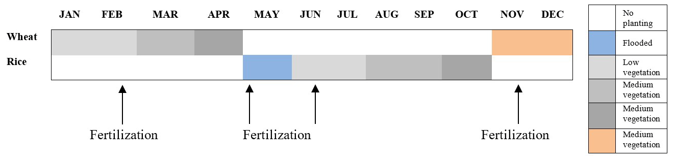
This observation was conducted at a site in Shouxian County in the eastern Chinese province of Anhui (32.42^∘ N, 116.76^∘ E) (Fig. 1). The altitude of the site is 27 m, and the annual mean air temperature and annual cumulative precipitation here are 16 ^∘C and 1115 mm, respectively. Summer (from June to September) precipitation accounts for nearly 60 % of the annual precipitation amount, which meets the high water demand of rice. Drought sometimes occurs due to lack of precipitation in the growing season of wheat. This observation site is rather flat, with farmland accounting for more than 90 % of the area. Winter wheat is grown here from November until late May, while from June to November the field is flooded, plowed, and harrowed as rice paddies (Duan et al., 2021a, b) (Fig. 2). The subtropical northern boundary of the monsoon humid climatic type describes the area's climate.

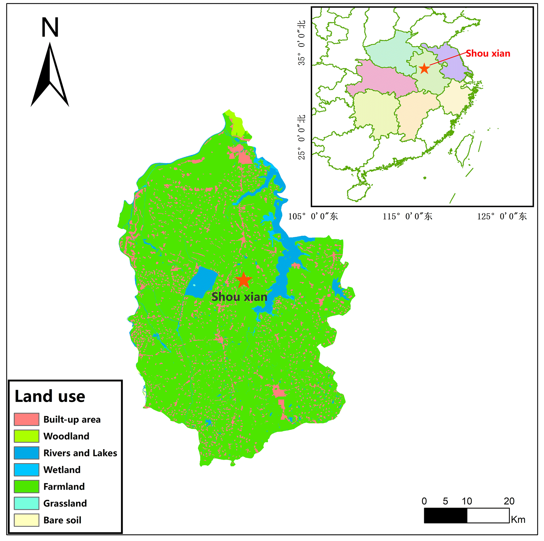
Figure 1 Geographical location and land cover map of Shouxian County.

Figure 2 Crop calendars for the rice and wheat in the North Yangtze River Delta region.

2.2 Data

Over the site described above, EC sensors (EC 150; Campbell Scientific Inc., Logan, UT, USA) were installed at 2.5 m above the ground, including a three-dimensional sonic anemometer (CSAT3; Campbell Scientific Inc., Logan, UT, USA) and a CO₂/H₂O open-path infrared gas analyzer. The sensible and latent heat fluxes were computed half-hourly using EddyPro software, with time lag compensation, double coordinate rotation, spectrum correction, and Webb–Pearman–Leuning density correction (Wutzler et al., 2018; Anapalli et al., 2019). Poor-quality fluxes (Eddypro quality check flag value of 2) were discarded. And a quality check based on the relationship between the measured flux and friction velocity was carried out to remove the biased data (Papale et al., 2006). Then, using the marginal distribution sampling technique, the flow data were gap filled (Reichstein et al., 2005). The time series of air temperature, relative humidity, wind speed, air pressure, friction velocity, and net radiation were also subjected to quality control. The missing data which need gap filling are H and LE, with 7205 and 16 013 missing, accounting for 12.09 % and 26.87 %, respectively. According to the criteria of $X\left(h\right)<(X-\mathrm{4}\mathit{\sigma })$ or $X\left(h\right)>(X+\mathrm{4}\mathit{\sigma })$, where X(h) indicates the time series of the component, X is the mean across the averaging interval, and σ is the standard deviation, noisy data were eliminated (Gao et al., 2003). Data observed from 15 July 2015 to 24 April 2019 are used in this study, and Fig. 3 shows the daily average data of R_n: net radiation (W m⁻²), u^∗: friction velocity (m s⁻¹), T: air temperature (^∘), RH: relative humidity (%), P: air pressure (hPa), and WS: wind speed (m s⁻¹).

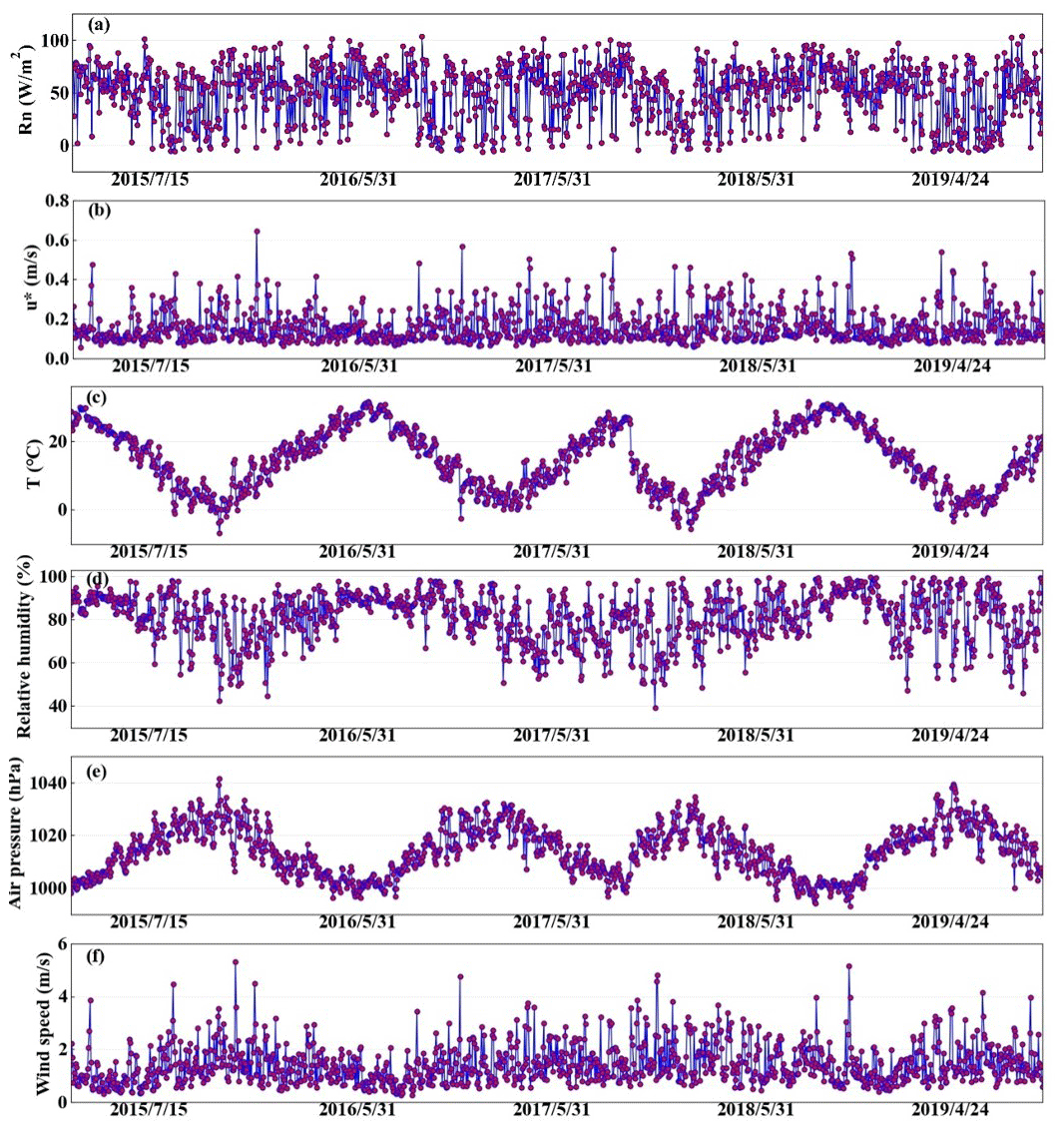
Figure 3 Daily averaged (a) R_n: net radiation (W m⁻²) , (b) u^∗: friction velocity (m s⁻¹), (c) T: air temperature (^∘), (d) RH: relative humidity (%), (e) P: air pressure (hPa), and (f) WS: wind speed (m s⁻¹).

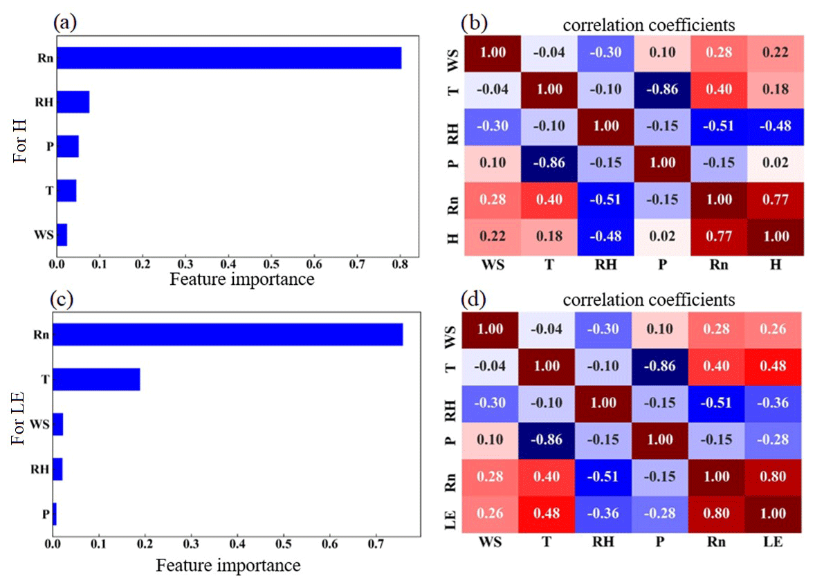
Figure 4 The feature importance of the variables for (a) H and (c) LE, and the correlation coefficient between each of the input variables for (b) H and (d) LE.

2.3 The RF model

RF is a machine learning method that is quick, adaptable, and frequently used to analyze classification and regression jobs (Breiman, 2001). This model can successfully evaluate highly dimensional and multicollinear data and is resistant to overfitting (Belgiu and Dragut, 2016). The RF model provides a feature selection tool to assist in determining the importance of the predictor. The contribution of each variable to the model, with important variables having a higher effect on the results of the model evaluation, is the definition of feature significance (Liu et al., 2021). Of the data, 90 % collected at the Shouxian observation site throughout the study period were used to train the RF model, while the remaining 10 % were used to independently validate the model (hereafter validation dataset). To lessen the overfitting in this case, a 10-fold cross-validation (CV) procedure was used (Cai et al., 2020). All training data used here were randomly divided into 10 subsamples of equal size for the 10-fold CV tests. And 9 out of the 10 subsamples were used as training data (hereafter training dataset), while the remaining subsample was used as testing data (hereafter testing dataset). All 10 of the subsamples were utilized as testing data exactly once for each of the 10 iterations of the CV procedure. One estimate was created by averaging the 10 findings from the folds. We modified the four RF model hyperparameters based on Bayesian optimization to get the optimal model (Baareh et al., 2021; Frazier, 2018): the maximum number of features considered to split a node (max features), the maximum number of trees to build (n estimators), the minimum sample number placed in a node prior to the node being split (min split), and the maximum number of levels for each decision tree (max depth). Bayesian optimizer is used to tune parameters, and you can quickly find an acceptable hyperparameter value; compared with grid search, the advantage is that the number of iterations is less (time saving), and the granularity can be very small. For example, if we want to adjust the regularized hyperparameters of linear regression, we set the black box function to linear regression, the independent variable is a hyperparameter, the dependent variable is linear regression in the training set accuracy, then set an acceptable black box function-dependent variable value, such as 0.95, and the obtained hyperparameter result is a hyperparameter that can make the linear regression accuracy exceed 0.95. The simulated performance of the 10-fold CV outcomes was evaluated using four statistical metrics: the correlation coefficient (r), mean absolute error (MAE), root mean square error (RMSE), and standard deviation (σ_n). As a result, the final RF model's parameters were adjusted as follows to have the best statistical metrics: n estimators is 246 min, split is 2, max features is 10, and max depth is 35.

The four statistical metrics are calculated by

$$\begin{array}{}\text{(1)}& {\displaystyle }r={\displaystyle \frac{\sum _{i=\mathrm{1}}^N\left(S_i-\stackrel{\mathrm{‾}}{S}\right)(O_i-\stackrel{\mathrm{‾}}{O})}{\sqrt{\sum _{i=\mathrm{1}}^N(S_i-\stackrel{\mathrm{‾}}{S}{)}^{\mathrm{2}}}\sqrt{\sum _{i=\mathrm{1}}^N(O_i-\stackrel{\mathrm{‾}}{O}{)}^{\mathrm{2}}}}},\text{(2)}& {\displaystyle }\mathrm{MAE}={\displaystyle \frac{\mathrm{1}}{N}}\sum _{i=\mathrm{1}}^N\left|S_i-O_i\right|,\text{(3)}& {\displaystyle }\text{RMSE}=\sqrt{{\displaystyle \frac{\sum _{i=\mathrm{1}}^N{\left(S_i-O_i\right)}^{\mathrm{2}}}{N}}},\text{(4)}& {\displaystyle }{\mathit{\sigma }}_n={\displaystyle \frac{\sqrt{\sum _{i=\mathrm{1}}^N(S_i-O_i{)}^{\mathrm{2}}}}{N}},\end{array}$$

where S stands for the modeled value, O is the observation, $\stackrel{\mathrm{‾}}{O}$ is the mean observed value, and $\stackrel{\mathrm{‾}}{S}$ is the mean modeled observation. σ_n indicates the standard deviation. The subscript i represents the serial number of samples, and N represents the total number of samples.

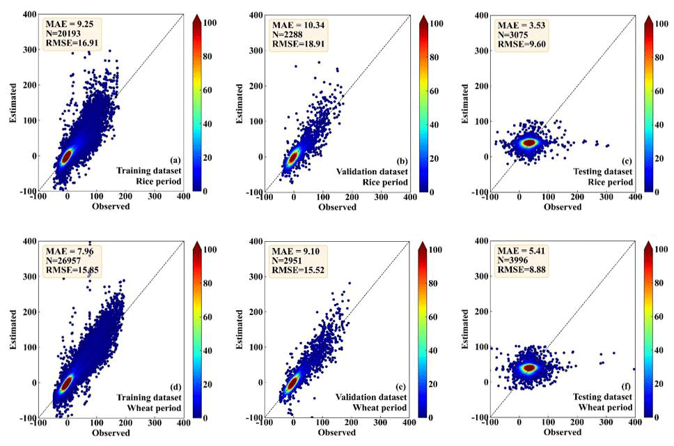
Figure 5 Scatter density plots of the observed and the RF-estimated H values, (a) and (d) for the training dataset, (b) and (e) for the validation dataset, and (c) and (f) for the testing dataset. And (a), (b), and (c) are in the period of rice, while (d), (e), and (f) are in the period of wheat.

3 Results and discussion

3.1 Driving factors of H and LE on a seasonal scale

The possible driving factors of H and LE were investigated to determine their respective contributions by the RF model, as shown in Fig. 4. R_n, which accounted for 78 % and 76 % of the total variable significance of H and LE, respectively, and was the most crucial variable in regulating the heat fluxes (Fig. 4a and c). Consistent with the high variable significance values, H and LE also had the highest r of 0.79 and 0.75 with H and LE, respectively, as shown in Fig. 4b and d. The other four factors contributed much less than R_n, and WS, T, RH, and P had importance values of 2 %, 4 %, 7 %, and 5 % (2.2 %, 19 %, 2 %, and 0.6 %) for H (LE), respectively. All these elements such as R_n, T, WS, RH are normalized before the model starts training. When these elements are normalized, it ensures uniformity and comparability. In general, all of these predictors played a role in the H and LE calculation, and for H, the sequence of importance was R_n, RH, P, T, and WS, while for LE, it was R_n, T, WS, RH, and P. The most significant impact on the change of H and LE came from R_n, which was the most important energy source of the surface and modulated the surface temperature directly. RH and T had a minor impact on the H and LE changes in terms of climatic parameters, which carried the information of the light-dependent reactions of H and LE fluxes. Particularly, WS and P had minimal impacts on the H and LE fluxes. The WS, T, and RH also affected H and LE according to the Monin–Obukhov similarity theory (Monin and Obukhov, 1954), while P represented the contributions from the background weather systems.

3.2 RF model evaluation

Figures 5–6 show the comparison between the observed and the RF-estimated H and LE, respectively. In the period of rice, the RF model showed good performance for both the training dataset (MAE is 8.51 and 17.89 W m⁻²; RMSE is 14.11 and 29.82 W m⁻², for H and LE, respectively) and the testing dataset (MAE is 9.61 and 10.34 W m⁻²; RMSE is 15.63 and 17.21 W m⁻², for H and LE, respectively) (Figs. 5a, b, 6a, and b). RF model also showed high consistency with direct measurements for the validation dataset (MAE is 5.88 and 20.97 W m⁻²; RMSE is 10.67 and 29.46 W m⁻², for H and LE, respectively), (Figs. 5c and 6c). In the period of wheat, the performance of the RF model for the training, testing, and validation datasets of H and LE was similar to that in the period of rice. For the training, testing, and validation datasets, respectively, the MAEs are 7.18, 8.01, and 6.01 W m⁻² for H, and 13.58, 8.82, and 19.93 W m⁻² for LE; and the RMSEs are 12.27, 13.61, and 9.86 W m⁻² for H, and 24.92, 15.17, and 28.74 W m⁻² for LE (Figs. 5d, e, f, 6d, e, f). These results demonstrate that the RF model is capable of effectively calculating the H and LE with input variables of R_n, WS, T, RH, and P.

3.3 Examination of input combinations

Meteorological elements may occasionally be unavailable due to the failure of sensors, so the five-variable input combination derived in Sect. 3.2 is not always applicable. Therefore, examination of other alternative input combinations is important to have substitute choices for data gap filling when the five-variable input combination is unavailable. In this subsection, we investigated the RF model's performance under the situation of lacking one element in the five-variable input combination; i.e., we tested the four-variable input combinations of (WS, T, RH, P), (R_n, T, RH, P), (R_n, WS, RH, P), (R_n, WS, T, P), and (R_n, WS, T, RH), by removing R_n, WS, T, RH, and P from the five-variable input combination, respectively. The MAEs and RMSEs for these combinations are shown in Table 1, and it demonstrates that the RF model's accuracy may either increase or decrease as a result of the removal of a meteorological element during the training phase. For instance, it was found that the model's performance greatly improved once RH was eliminated from the input combination, with the MAE and RMSE of H decreasing from 6.48 and 11.94 W m⁻² to 5.66 and 11.06 W m⁻², respectively, and LE from 19.1 and 39.39 W m⁻² to 17.74 and 35.27 W m⁻². This outcome is logical given that RH and H do not have a strong correlation; as a result, performance will be enhanced if RH is not included in the gap-filling processing pipeline. According to our findings, the RF model's performance may be greatly enhanced by excluding irrelevant meteorological elements from the study and choosing only those that have a significant impact on the variable. Our findings imply that in order to attain the best gap-filling accuracy, it is necessary to take into account both the advantages and disadvantages of ML-based models and the ideal input components. The results suggested that RH at a single level was not well correlated to the fluxes as shown in Sect. 3.1, because the one-level RH was strongly affected by the irrigation activity which was an external factor of the weather system. As a result, RF model performance was enhanced when the irrelevant variable (i.e., RH) was removed from the input list. The same condition also happened to the removal of WS, as could be seen from Sect. 3.1, WS showed small correlations with the fluxes. WS over this site was rather small, and frequently below 2 m s⁻¹, and under this light wind condition, the fluxes were mostly driven by the buoyancy rather than the wind shear. Figure 7 presents the MAE variation percentage of the four-variable input combinations from the five-variable input combination. After RH was removed from the input list, the RF model showed favorable performance for both H and LE, as shown in Fig. 7, with MAE values improvements of 12.65 % and 7.12 %, respectively. Notably, the removal of R_n from the input combination resulted in a considerable decline in the RF model's performances, with MAE degradation percentage values reaching 16.20 % and 10.73 %, respectively. This outcome makes sense, since R_n is highly associated with H and LE; hence, performance will be declined if R_n is left out of the input training dataset. As a consequence, our findings demonstrated that choosing strongly associated components could greatly increase the gap-filling accuracy. According to our findings, the best input combination is [R_n, WS, T, P].

Figure 6 Same as Fig. 5 but for LE.

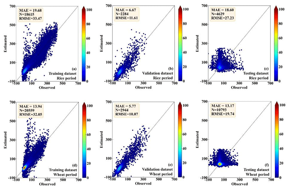
Table 1 The MAEs and RMSEs of the RF-estimated heat fluxes for the four-variable input combinations, and the corresponding changes from the five-variable input combination.

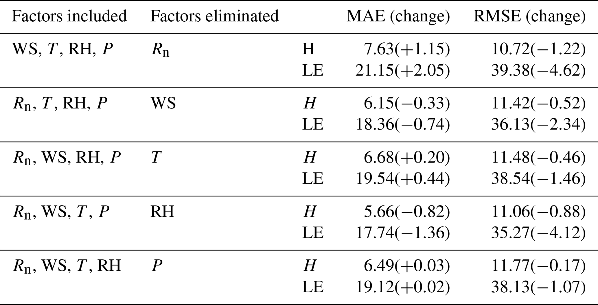
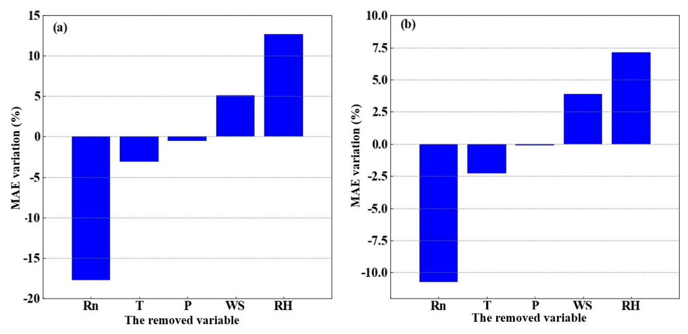
Figure 7 The MAE percentage variation after changing the five-variable input combinations to the four-variable input combinations, (a) for H and (b) for LE, respectively. The x axis labels indicate the removed variables.

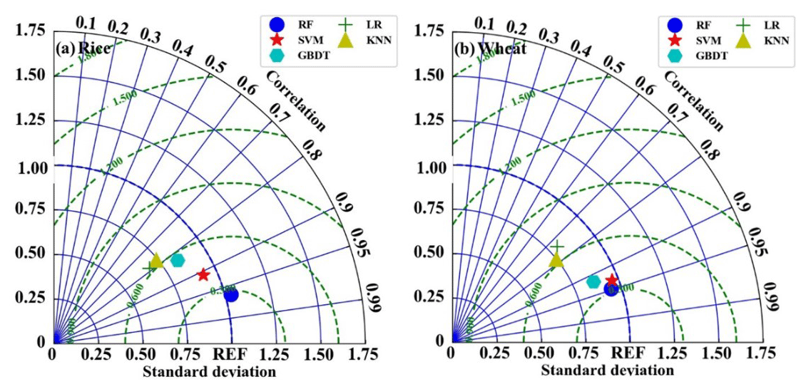
Figure 8 The performances of the five models for estimating H in the period of (a) rice and (b) wheat.

Figure 9 The same as in Fig. 8 but for LE.

It should be noted that other variables that might have an impact on the H and LE were not investigated here. For example, given that our research site was over farmland and plants were growing, knowledge of the variations of the leaf area index (LAI) and inclusion of it to the training dataset should also be useful to increase the accuracy of the RF model in H and LE gap filling. The monsoonal climate here also incurred considerable precipitation variations, which might as well potentially contribute to the RF model accuracy improvement. However, due to the lack of LAI and precipitation observations, the inclusion of the two variables into the RF model training dataset was not applicable in this study. Additionally, as shown above, more variables would bring a higher observation demand and lead to more complexity and potentially decreased results, such as the adding variable of RH.

3.4 Comparison with other four ML methods

3.4.1 Comparison in H estimation

To further investigate the reliability of the RF model, we used a Taylor diagram to compare its performance in H estimation with the other four ML models: support vector machine (SVM), k nearest-neighbor (KNN), gradient boosting decision tree (GBDT), and linear regression (LR). SVM is a data-oriented classification algorithm, and the basic model is to find the best separation hyperplane on the feature space so that the positive and negative sample intervals on the training set are maximum. Its advantages are that the kernel function can be used to map to a high-dimensional space; the use of the kernel function can solve the nonlinear classification; the classification idea is very simple, that is, to maximize the interval between the sample and the decision-making surface; the classification effect is better; and the nonlinear relationship between data and features is easy to obtain when the small and medium-sized sample size is large. KNN is particularly suitable for multi-classification problems. Its advantage is that it is simple in thought, easy to understand, and easy to implement; there are no estimation parameters and no training – it is highly accurate and insensitive to outliers. GBDT can flexibly handle various types of data, including continuous and discrete values. With relatively few parameter adjustment times, the prediction preparation rate can also be relatively high. If the data dimension is high, the computational complexity of the algorithm will increase. Using some robust loss functions, the robustness to outliers is very strong. LR is a statistical analysis method that uses regression analysis in mathematical statistics to determine the quantitative relationship between two or more variables that depend on each other.The results have good interpretability, can intuitively express the importance of each attribute in the prediction, and the calculation of entropy is not complicated.

All the models were optimized with the same technique described above for the RF model. The results are shown in Fig. 8. The EC measurements were used as the benchmark. It can be seen that the RF model generally outperforms the other four models, with standard deviations (σ_n) and correlation values of 1.05 and 0.98 during the period of rice planting and 0.96 and 0.95 during the period of wheat planting, respectively. The SVM model is the second most accurate model, with a σ_n and correlation of 0.92 and 0.98 during the period of rice planting and 0.91 and 0.93 during the period of wheat planting, respectively. The LR model performs the worst, with a σ_n and correlation of 0.60 and 0.76 during the period of rice planting and 0.80 and 0.72 during the period of wheat planting, respectively. The accuracy of KNN and the GBDT models is in between the above-discussed models, and the σ_n and correlation during the rice and wheat period for KNN is 0.68 and 0.73 and 0.77 and 0.82; for GBDT, it is 0.79 and 0.80 and 0.81 and 0.9, respectively.

3.4.2 Comparison in LE estimation

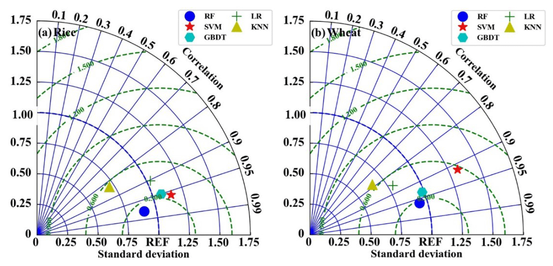
Figure 9 illustrates a comparison of the estimated LE by all five models during the period of rice and wheat planting. The results are similar to those in the H estimation, and the RF model is found to perform better than the other four models, with σ_n and correlation values of 0.95 and 0.97 during the period of rice planting and 0.97 and 0.96 during the period of wheat planting, respectively. Nonetheless, the KNN model performs the worst for LE estimating, and it has σ_n and correlation values of 0.68 and 0.82 during the period of rice planting and 0.62 and 0.79 during the period of wheat planting, respectively. Overall, as shown by the Taylor diagram of Figs. 8 and 9, in this study, the RF model has the best accuracy in either H or LE estimation for data gap filling.

4 Summary and conclusions

To assess the RF model's capacity for gap filling the sensible and latent heat flux measurements over rice–wheat rotation croplands, 90 % of the total observation data gathered at Shouxian were utilized for training and testing, and the remaining 10 % of data were used for independent validation. Our findings demonstrate that R_n is the most important variable in regulating H and LE, and it accounts for 78 % and 76 % of the total variable significance in the RF model construction for H and LE calculation, respectively. The least important variables are WS and P, and their total variable significance is 2 % and 0.6 %, respectively. During the periods of rice and wheat planting, the RF model with a five-variable input combination shows reliable performance, with MAE values of 5.88 and 20.97 W m⁻² and RMSE values of 10.67 and 29.46 W m⁻², respectively. However, further analysis of the RF model with four-variable input combinations indicates that the performance of the model is improved when RH is removed from the input list, and the MAE values decrease by 12.65 % and 7.12 % for H and LE, respectively. Nonetheless, the four-variable input combination without R_n causes an increase in the MAE values of the model, by 16.20 % and 10.73 % for H and LE, respectively. Therefore, the best input combination found in this study for heat flux gap filling is [R_n, WS, T, P]. Statistical comparison of RF and other four typical ML models (LR, KNN, SVN, and GBDT) by Taylor diagram further shows that RF is the most accurate, with the standard deviations and correlation values of 0.95 and 0.97 during the period of rice planting and 0.97 and 0.96 during the period of wheat planting, respectively. On the other hand, the LR and KNN models perform the worst for H and LE gap filling, respectively, according to the statistical metrics of the Taylor diagram.

This study is based on only the data collected over rice–wheat rotation croplands, but the method presented above to find a reliable gap-filling ML model can also be used over other types of underlying surfaces and in other climate zones. It should be noted that over different types of underlying surfaces and climates, the variable significance can vary, and a careful check of the input combinations is needed. For example, over polar oceans with strong winds, R_n probably is not the most important driving factor, while the winds which cause mostly the turbulence may take the first place. On the other hand, over areas without human irrigation activity, RH will possibly be strongly related to the latent heat flux, and hence the inclusion of it in the input list may increase the ML model performance. Besides the examination of the input combinations, the choice of an ML model and the method to optimize its parameters are also important.

Overall, this study shows the potential to use the RF model to produce trustworthy gap-filling data of H and LE over rice–wheat rotation croplands, and the ML methods are suggested to be used to derive the fluxes' estimations when direct EC observations are not available.