Estimation of NO₂ emission strengths over Riyadh and Madrid from space from a combination of wind-assigned anomalies and a machine learning technique

Nitrogen dioxide (NO₂) air pollution provides valuable information for quantifying NO_x (NO_x = NO + NO₂) emissions and exposures. This study presents a comprehensive method to estimate average tropospheric NO₂ emission strengths derived from 4-year (May 2018–June 2022) TROPOspheric Monitoring Instrument (TROPOMI) observations by combining a wind-assigned anomaly approach and a machine learning (ML) method, the so-called gradient descent algorithm. This combined approach is firstly applied to the Saudi Arabian capital city of Riyadh, as a test site, and yields a total emission rate of 1.09×10²⁶ molec. s⁻¹. The ML-trained anomalies fit very well with the wind-assigned anomalies, with an R² value of 1.0 and a slope of 0.99. Hotspots of NO₂ emissions are apparent at several sites: over a cement plant and power plants as well as over areas along highways. Using the same approach, an emission rate of 1.99×10²⁵ molec. s⁻¹ is estimated in the Madrid metropolitan area, Spain. Both the estimate and spatial pattern are comparable with the Copernicus Atmosphere Monitoring Service (CAMS) inventory.

Weekly variations in NO₂ emission are highly related to anthropogenic activities, such as the transport sector. The NO₂ emissions were reduced by 16 % at weekends in Riyadh, and high reductions were found near the city center and in areas along the highway. An average weekend reduction estimate of 28 % was found in Madrid. The regions with dominant sources are located in the east of Madrid, where residential areas and the Madrid-Barajas airport are located. Additionally, due to the COVID-19 lockdowns, the NO₂ emissions decreased by 21 % in March–June 2020 in Riyadh compared with the same period in 2019. A much higher reduction (62 %) is estimated for Madrid, where a very strict lockdown policy was implemented. The high emission strengths during lockdown only persist in the residential areas, and they cover smaller areas on weekdays compared with weekends. The spatial patterns of NO₂ emission strengths during lockdown are similar to those observed at weekends in both cities. Although our analysis is limited to two cities as test examples, the method has proven to provide reliable and consistent results. It is expected to be suitable for other trace gases and other target regions. However, it might become challenging in some areas with complicated emission sources and topography, and specific NO₂ decay times in different regions and seasons should be taken into account. These impacting factors should be considered in the future model to further reduce the uncertainty budget.

1 Introduction

Nitrogen oxides (NO_x = NO + NO₂) are a group of highly reactive trace gases (NO and NO₂). These gases are toxic to human health and play a key role in tropospheric chemistry by catalyzing tropospheric O₃ formation and acting as aerosol precursors, and this tropospheric O₃ is a secondary pollutant that is also harmful to human health (IPCC, 2021). The emission of NO_x is dominated by human activities and is mostly related to fossil fuel or biomass combustion (Goldberg et al., 2019). The major anthropogenic source in Europe is road transport (39 %), followed by another four sectors with similar shares: energy production and distribution (14 %); commercial, institutional, and households (13 %); energy use in industry (11 %); and agriculture (11 %) (EEA, 2021). The near-surface abundance of NO_x has generally increased with urbanization and industrialization (IPCC, 2021; Barré et al., 2021). Additionally, due to its short tropospheric lifetime (1–12 h) (Beirle et al., 2011; Stavrakou et al., 2013), NO_x concentrations are highly variable and strongly correlated with local emission sources (Goldberg et al., 2019). Thus, NO₂ observations can be considered as an excellent indicator of NO_x emissions. For this reason, accurate knowledge of the spatial and temporal distribution of NO₂ atmospheric abundances is critical.

Space missions succeed in delivering well-resolved maps of tropospheric NO₂ columns, such as the early Global Ozone Monitoring Experiment (GOME) (Burrows et al., 1999), the widely used Ozone Monitoring Instrument (OMI) (Boersma et al., 2007; He et al., 2020), and the latest TROPOspheric Monitoring Instrument (TROPOMI) (Veefkind et al., 2012). Among them, TROPOMI, which has operated aboard Sentinel-5 Precursor (S5P) since October 2017, has an outstanding importance. It is a push-broom grating spectrometer and measures direct and reflected sunlight in the ultraviolet, visible, near-infrared, and shortwave infrared bands (Veefkind et al., 2012). TROPOMI offers daily coverage of data with an unprecedented spatial resolution of 3.5×7 km² (3.5×5.5 km² since August 2019) and a high signal-to-noise ratio (van Geffen et al., 2021). The TROPOMI NO₂ data have been used for a variety of studies to estimate the NO_x lifetime and emissions. For example, Lorente et al. (2019) demonstrated that the strength and distribution of NO₂ emissions from Paris can be directly determined from TROPOMI NO₂ measurements. Beirle et al. (2019) mapped NO_x emissions at a high spatial resolution based on the continuity equation and quantified urban pollution from Riyadh, Saudi Arabia (8.5 kg s⁻¹ over 250×250 km²). A top-down NO_x emission estimate approach was developed by Goldberg et al. (2019), who reported that three megacities (New York City, Chicago, and Toronto) in North America emitted 3.9–5.3 kg s⁻¹ NO_x. Liu et al. (2020) demonstrated a 48 % drop in the tropospheric NO₂ column densities in China during the COVID-19 lockdown. The reductions in NO₂ emissions across the European urban areas resulting from the lockdown were studied by Barré et al. (2021), and −23 % changes on average were obtained based on TROPOMI NO₂ observations.

TROPOMI is unique due to its very high spatial and temporal resolution and provides a large number of data despite a planned mission lifetime of only about 4 years. This huge data set offers the possibility of exploitation by quickly developed artificial intelligence machine learning (ML) techniques. For example, the application of ML to assess the NO₂ pollution changes during the COVID-19 lockdown (Petetin et al., 2020; Keller et al., 2021; Barré et al., 2021; Chan et al., 2021). However, to date, most studies have focused on changes in the NO₂ column abundances. The accurate amount and spatial pattern of deduced emission strengths are also important and can aid air quality policy development.

In this study, the gradient descent (GD) ML approach incorporating the wind-assigned method (Tu et al., 2022a, b) is used to train the “modeled truth”, constructed from a simple downwind plume model for the emissions in each grid pixel using spaceborne NO₂ observations, in order to estimate the NO₂ emission strengths of two (mega)cities: Riyadh (Saudi Arabia) and Madrid (Spain). The rest of the paper is organized as follows. Section 2 presents the data set and the combined method (wind-assigned and ML methods). The approach is applied to the Saudi Arabian capital city Riyadh for its evaluation and then to Madrid; this is followed by a discussion of the differences on weekdays and at weekends as well as the changes before and during the COVID-19 lockdown period (Sect. 3). Conclusions are given in Sect. 4.

2 Data and methodology

2.1 TROPOMI tropospheric NO₂ columns and wind data

The NO₂ data used in this study were obtained from the Sentinel-5P Pre-Operations Data Hub (https://s5phub.copernicus.eu/dhus/#/home, last access: 18 April 2023), which provides level-2 data sets with three different data streams: the Non-Time-Critical or Offline (OFFL), the Reprocessing (RPRO), and the Near-real-time (NRTI) streams. The NRTI stream is available within 3 h after the actual satellite measurement, may sometimes be incomplete, and has a slightly lower data quality (http://www.tropomi.eu/data-products/level-2-products, last access: 14 September 2022); thus, this data set is not considered here. The RPRO data cover a time range from 30 April 2018 to 17 October 2018, and the OFFL data cover the remaining time period. Meanwhile, the NO₂ data set is an aggregate of different versions. The RPRO data are v1.2, whereas OFFL data include several versions: v1.2 until 20 March 2019, v1.3 until 29 November 2020, v1.4 until 5 July 2021, v2.2 until 15 November 2021, v2.3 until 17 July 2022, and v2.4 after 17 July. An improved FRESCO (Fast Retrieval Scheme for Clouds from the Oxygen A-band) cloud retrieval has been introduced in v1.4, which leads to higher tropospheric NO₂ columns over areas with pollution sources under a small but nonzero cloud coverage (van Geffen et al., 2022). We used the TROPOMI tropospheric NO₂ from May 2018 to June 2022 over the Saudi Arabian capital city of Riyadh and another (mega)city in Europe, namely Madrid (Spain). A quality flag (qa_value) value of >0.75 is recommended, as data are thereby restricted to cloud-free (cloud radiance fraction <0.5) and snow- and ice-free observations (van Geffen et al., 2021). There are nearly 1 380 000 good-quality measurements in Riyadh (23.6–25.4^∘ N, 46.1–47.4^∘ E) and 930 000 good-quality measurements in Madrid (39.5–41.5^∘ N, 4.5–3^∘ W) over 4 years. These observations are then binned on a regular $\mathrm{0.1}{}^{\circ }\times \mathrm{0.1}{}^{\circ }$ grid for this study with the prerequisite that the number of observations is larger than five in the respective grid point. The number of TROPOMI measurements in each 0.1^∘ grid pixel is distributed evenly with a number range of 4400–4800 in Riyadh, whereas larger differences are observed in Madrid with a number range of 2200–3700 (see Fig. A1).

We use the horizontal wind information from ERA5, which is the fifth-generation climate reanalysis produced by the European Centre for Medium-Range Weather Forecasts (ECMWF) at a spatial resolution of $\mathrm{0.25}{}^{\circ }\times \mathrm{0.25}{}^{\circ }$ (Copernicus Climate Change Service, 2017). NO₂ is a short-lived species, and its level can be easily influenced by the orography; therefore, we use ERA5 at 10 m.

2.2 Wind-assigned and ML methods

The averaged distribution of emitted NO₂ over a long-term period can be approximated by an evenly distributed cone-shaped plume, which is prescribed by wind speed and direction, and source strength with consideration of its temporal decay:

$$\begin{array}{}\text{(1)}& \mathrm{\Delta }{\mathrm{NO}}_{\mathrm{2}(xi,yi)}={\displaystyle \frac{\mathit{\epsilon }}{v\cdot d_{(xi,yi)}\cdot \mathit{\alpha }}}\times \exp \left(-{\displaystyle \frac{t}{\mathit{\tau }}}\right),\end{array}$$

where ε is the emission strength and has an initialized value of 1×10²⁶ molec. s⁻¹. The study area is binned on a regular $\mathrm{0.1}{}^{\circ }\times \mathrm{0.1}{}^{\circ }$ grid, and the emission rates at each grid are assumed to be constant during the study period. α is the angle of the emission cone and has an empirical value of $\mathrm{1}/\mathrm{3}$ rad (i.e., 60^∘) (Tu et al., 2022a). d and t are the distance in meters and the transport time in hours between the downwind location and the NO₂ emission source, respectively. v is the wind speed in meters per second from ERA5, and τ is the lifetime/decay time in hours for NO₂. For simplification, seasonal and spatial variability in the lifetime is not considered, and empirical values based on Beirle et al. (2011, 2019), i.e., fixed values of 4 h for Riyadh and 7 h for Madrid, are used in this study. The daily plumes (ΔNO₂) from the individual emission source are computed based on Eq. (1) and are then superimposed to obtain a total daily plume. The ERA5 model wind is divided into two opposite wind regimes based on the predominant wind regimes at each site (i.e., S is 90–270^∘ and N is the rest for Riyadh, whereas SW is 135–315^∘ and NE is the rest for Madrid; see Fig. A2). A temporally averaged ΔNO₂ plume is obtained for each wind regime, and the difference between the two plumes generates the wind-assigned anomalies (for more details, the reader is referred to Tu et al., 2022a, b).

The study area has x×y (=N) grids. Each grid cell is considered to be an independent point source at position $s_{{\mathrm{lat}}_i},s_{{\mathrm{lat}}_j}$, which yields a map of wind-assigned anomalies (${\mathit{c}}_{s_{{\mathrm{lat}}_i},s_{{\mathrm{lat}}_j}}$). The wind information is assumed to be constant at each time over the study area in this study. The modeled wind-assigned anomalies derived from the point source located at the center grid (${\mathrm{lat}}_{i_{\mathrm{0}}},{\mathrm{long}}_{j_{\mathrm{0}}}$) are considered to be a parent map (see Fig. A3a):

$$\begin{array}{}\text{(2)}& {\mathit{c}}_{s_{{\mathrm{lat}}_{i_{\mathrm{0}}}},s_{{\mathrm{lat}}_{j_{\mathrm{0}}}}}=\left(p_{{\mathrm{lat}}_{\mathrm{1}},{\mathrm{long}}_{\mathrm{1}}}\mathrm{\cdots }{p}_{{\mathrm{lat}}_i,{\mathrm{long}}_j}\mathrm{\cdots }{p}_{{\mathrm{lat}}_x,{\mathrm{long}}_y}\right).\end{array}$$

The anomalies derived from other point sources are identical to the parent anomalies, and the value at each grid depends on the location relative to the parent location (see Fig. A3b):

$$\begin{array}{}\text{(3)}& \begin{array}{rl}& {\mathit{c}}_{s_{{\mathrm{lat}}_i},s_{{\mathrm{long}}_j}}=(p_{{\mathrm{lat}}_{\mathrm{1}}-{\mathrm{lat}}_{i_{\mathrm{0}}},{\mathrm{long}}_{\mathrm{1}}-{\mathrm{long}}_{i_{\mathrm{0}}}}\mathrm{\cdots }{p}_{{\mathrm{lat}}_i-{\mathrm{lat}}_{i_{\mathrm{0}}},{\mathrm{long}}_j-{\mathrm{long}}_{i_{\mathrm{0}}}}\mathrm{\cdots }\\ & p_{{\mathrm{lat}}_x-{\mathrm{lat}}_{i_{\mathrm{0}}},{\mathrm{long}}_y-{\mathrm{long}}_{i_{\mathrm{0}}}}).\end{array}\end{array}$$

These maps of wind-assigned anomalies at each grid are input for the further step, which needs to be reformatted. The locations of the grids are reordered in the sequence of latitude and longitude values from west to east and from north to south. The first grid at lat₁,long₁ is located in the far northwest, and the last grid at lat_x,long_y is located in the far southeast. Therefore, each map of wind-assigned anomalies is converted to a new column vector ${\mathit{c}}_k={\left(a_{k,\mathrm{1}}\mathrm{\cdots }{a}_{k,N}\right)}^{\mathit{T}}$, i.e., a_k,k represents the wind-assigned anomalies at the kth grid cell derived from point sources at the kth grid cell. The N grids generate N vectors to construct an N × N matrix:

$$\begin{array}{}\text{(4)}& \mathbf{M}=\left({\mathit{c}}_{\mathrm{1}}\mathrm{\cdots }{\mathit{c}}_N\right)=\left(\begin{array}{lll}{a}_{\mathrm{1},\mathrm{1}}& \mathrm{\cdots }& a_{N,\mathrm{1}}\\ \mathrm{⋮}& \mathrm{\ddots }& \mathrm{⋮}\\ a_{\mathrm{1},N}& \mathrm{\cdots }& a_{N,N}.\end{array}\right)\end{array}$$

The estimated emission rate is a column vector w=(w₁⋯w_N)^T. As the emission rates cannot be negative, we use log(w_k) as a proxy for the w_k. The final result is then the exponent of the log(w_k) and scaled by the initial ε of 1×10²⁶ molec. s⁻¹. The model-calculated map (m) of the wind-assigned anomalies can then be written as follows:

$$\begin{array}{}\text{(5)}& \begin{array}{rl}\mathit{m}& =\mathbf{M}\times \mathit{w}=\left(\begin{array}{lll}{a}_{\mathrm{1},\mathrm{1}}& \mathrm{\cdots }& a_{N,\mathrm{1}}\\ \mathrm{⋮}& \mathrm{\ddots }& \mathrm{⋮}\\ a_{\mathrm{1},N}& \mathrm{\cdots }& a_{N,N}\end{array}\right)\times (w_{\mathrm{1}}\mathrm{\cdots }{w}_N{)}^{\mathit{T}}\\ & =(m_{\mathrm{1}}\mathrm{\cdots }{m}_N{)}^{\mathit{T}}.\end{array}\end{array}$$

The wind-assigned anomaly method is also applied to the TROPOMI tropospheric NO₂ column, yielding a true map y=(y₁⋯y_N)^T.

To estimate the emission strengths accurately, the modeled map (m) should approximate the true map (y). This problem is then converted to find the best w which results in the minimum value of the difference between y and m, i.e., the cost function:

$$\begin{array}{}\text{(6)}& \begin{array}{rl}& L\left(\mathit{y}\mathbf{,}\mathit{m}\right)={\displaystyle \frac{\mathrm{1}}{N}}\sum _{i=\mathrm{1}}^N{\left(y_i-m_i\right)}^{\mathrm{2}}=\\ & {\displaystyle \frac{\mathrm{1}}{N}}\sum _{i=\mathrm{1}}^N{\left(y_i-\left(a_{\mathrm{1},i}\mathrm{\cdots }{a}_{N,i}\right)\times (w_{\mathrm{1}}\mathrm{\cdots }{w}_N{)}^{\mathit{T}}\right)}^{\mathrm{2}}.\end{array}\end{array}$$

In our approach, the above equation can be considered to solve a linear system with constraints over the coefficients. In the ML framework, the popular GD algorithm can be a simple yet effective solution to find the coefficients. These coefficients can satisfy the approximation and the constraints at the same time by formulating some of the constraints into the loss function that needs to be optimized. The main idea of GD is to find the partial derivatives of all coefficients in the system with respect to the loss function and to use the local (gradient) information to reach a solution closer to the true state, which minimizes the approximation loss. In practice, this is implemented using an iterative process in which the data are sampled for the required gradients. However, there is only one single “data point” (one column vector) in our problem formulation. For each iteration (Eq. 7), the new weight (w_t+1) is equal to the old weight (w_t) minus the gradient multiplied by the learning rate η (or the so-called step size). Here, we use the default settings (η=0.001) as employed by Kingma and Ba (2015):

$$\begin{array}{}\text{(7)}& {\mathit{w}}_{t+\mathrm{1}}={\mathit{w}}_t+\mathrm{\Delta }{\mathit{w}}_t={\mathit{w}}_t-\mathit{\eta }\times \sum _{i=\mathrm{1}}^N{\displaystyle \frac{\mathit{\delta }L}{\mathit{\delta }{\mathit{w}}_t}}.\end{array}$$

The selected areas in this study are highly isolated from the neighboring sources; thus, the emission rates at the edge can be assumed to be zero. However, the initial constraint of the sources can increase the final biases. Therefore, we use a larger study area with (n+2) × (m+2) grids as the input data and remove the outmost rectangle within a two-grid width of the target area of n×m grids.

When applying GD to complicated systems with many parameters, there are many variations of GD that do not only rely on the gradients but also introduce additional temporal information (i.e., the accumulation of gradients over time, known as “momentum”) to help GD converge more quickly and reliably. Among those algorithms, we decided to use Adaptive Moment Estimation (ADAM), as it is characterized by enhanced efficiency and low cost requirements (Kingma and Ba, 2015) compared with second-order methods such as BFGS (Broyden–Fletcher–Goldfarb–Shanno); moreover, for our problem, it can slightly outperform other GD variations, such as the original gradient descent (GD) with momentum or Adadelta/Adagrad. In addition, it has been documented that ADAM is superior because it employs the cumulative first-order and second-order moments; thus, it has become the de facto method in the current deep learning scene when dealing with large numbers of data and parameters (Kingma and Ba, 2015).

3 Results and discussion

3.1 Testing approaches for NO₂ emission estimation in Riyadh

Riyadh was chosen as the test site because this city, located in an area that experiences an arid climate, has high NO_x emissions, due to the high population density (∼4300 residents per square kilometer; https://worldpopulationreview.com/world-cities/riyadh-population, last access: 29 March 2022), and strong point sources of NO_x close to the metropolitan area, such as a cement plant and power plants. Moreover, Riyadh is remote from other sources and has favorable weather conditions for space-based measurements, such as low cloud cover and high surface albedo (Beirle et al., 2019; Rey-Pommier et al., 2022). The two typical wind regimes present in Riyadh favor the applicability of the wind-assigned anomaly method and are another reason for choosing this region for this work.

Figure 1 illustrates the averaged wind-assigned plumes derived from the TROPOMI tropospheric NO₂ and the ML method over the analyzed period (May 2018–June 2022). The ML-modeled plumes show excellent agreement with the satellite results (true map). A stronger plume is observed in the south of Riyadh, as the wind more often comes from the north (Fig. A2a, b). The good correlation between these two maps is also presented in the one-to-one figure (Fig. 1c), with an R² value of 1.0 and a slope value of 0.99. The estimated emission strengths based on the ML model (Fig. 1d) show a similar spatial pattern, especially for the main sources near the city center, to the results in Beirle et al. (2019) (Fig. 2). Hotspots of NO₂ emissions are apparent at several sites: over a cement plant and power plants as well as over areas along the highways (Fig. 1d). These power plants have capacities larger than 1 GW and use crude oil and partly natural gas as fossil fuels (Beirle et al., 2019). The total emission rate is about 1.09×10²⁶ molec. s⁻¹. Our estimate is slightly higher than the results of Beirle et al. (2019) (8.3×10²⁵ molec. s⁻¹ from December 2017 to October 2018), who used wind fields from the ECMWF operational analysis at about 450 m above the ground. This difference might be due to the different study periods and methods used. The pattern of wind direction is similar at a higher level (100 m), while the wind speed increases (Fig. A2a, b, c); therefore, it is expected that wind at these levels has minor impacts on the estimates.

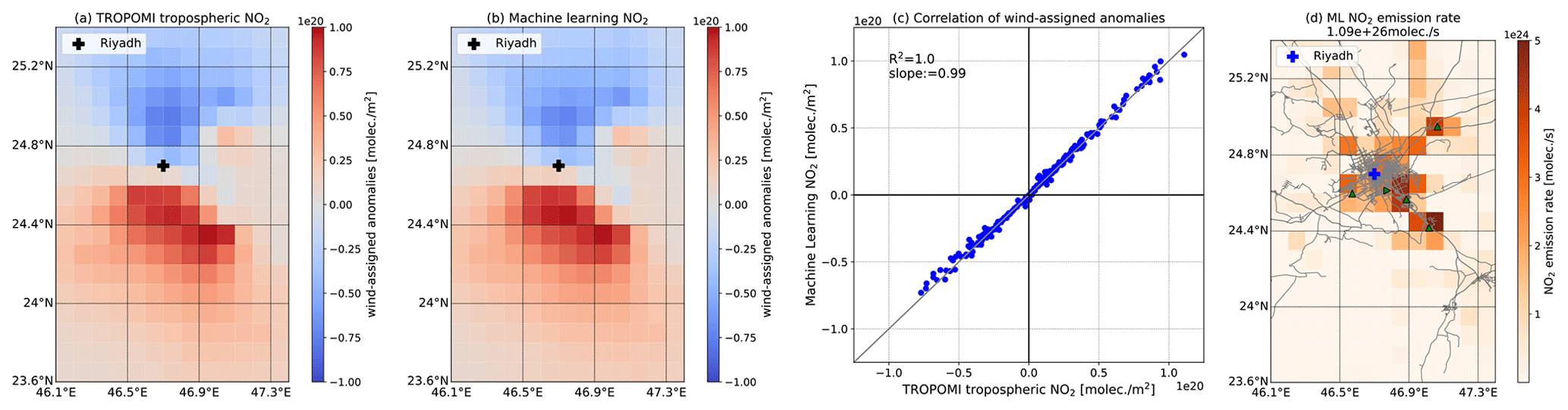
Figure 1 Wind-assigned plumes derived from (a) TROPOMI tropospheric NO₂ and (b) the ML method; (c) a correlation plot between (a) and (b) for each grid (where the x and y labels represent the data sets from which the wind-assigned anomalies were derived); and (d) the estimated emission rates in Riyadh, Saudi Arabia. The data in panels (a), (b), and (d) are gridded on a regular latitude–longitude grid with 0.1^∘ spacing. In panel (d), the number in the panel heading presents the total emission rate; triangle symbols and the right-pointing triangle symbol represent power plants and a cement plant, respectively; gray lines represent the highways (data derived from https://www.openstreetmap.org (last access: 19 April 2023), © OpenStreetMap, and https://www.mapcruzin.com, last access: 11 April 2022).

3.2 NO₂ emission in Madrid

As a (mega)city in Europe, Madrid (Spain) is another target in this study. The population of the Madrid metropolitan area is estimated to be about 6.7 million, and nearly half of the residents live in Madrid city, resulting in a population density of ∼5400 residents per square kilometer (https://worldpopulationreview.com/world-cities/madrid-population, last access: 29 March 2022). Figure 2a and b display the wind-assigned anomalies derived from TROPOMI observations and the ML method, showing clearly pronounced bipolar plumes that are symmetrical in the Madrid city center. The ML-trained anomalies show very good agreement with the TROPOMI values, with an R² value of 0.99 and a slope of 0.98 (Fig. 2c). The spatial pattern of estimated emission strengths is shown in Fig. 2d and is comparable to that of the CAMS-REG-AP (Copernicus Atmospheric Monitoring Service regional anthropogenic emission inventory, https://eccad.aeris-data.fr/catalogue/, last access: 31 March 2022; Granier et al., 2019; Kuenen et al., 2021) (Fig. 2e). CAMS-REG-AP covers emissions from the United Nations Economic Commission for Europe (UNECE) for the main air pollutants (e.g., NO_x, expressed as NO₂) with a spatial resolution of $\mathrm{0.05}{}^{\circ }\times \mathrm{0.1}{}^{\circ }$ to $\mathrm{0.1}{}^{\circ }\times \mathrm{0.1}{}^{\circ }$ in longitude and latitude on a yearly basis over Europe (Kuenen et al., 2014). CAMS-REG-v5.1 BAU 2020 is the latest version of a series of emission inventories that extrapolate CAMS-REG-v5.1 to the year 2020, neglecting the impacts related to COVID-19 (Kuenen et al., 2021). CAMS-REG-v5.1 covers the data from 2000 to 2018, and CAMS-REG-v4.2-ry covers the updated recent years of 2018 and 2019 (https://eccad3.sedoo.fr/#CAMS-REG-AP, last access: 17 August 2022). The total emission rate over the whole study is about 1.90×10²⁵ molec. s⁻¹, which is close to the CAMS inventory value of 1.12×10²⁵ molec. s⁻¹ in 2020.

Our estimate is lower than a previous estimate of 6.8×10²⁵ molec. s⁻¹ derived from OMI data during 2005–2009 (Beirle et al., 2011). The time series of tropospheric NO₂ observed by OMI since 2004 and TROPOMI since 2018 at two study sites are shown in Fig. A13, and their correlations are shown in Fig. A14. In Riyadh, NO₂ amounts increased from 2004 and reached their highest value in around 2016, except for a sudden drop in 2013. A continuous decrease is observed in Madrid except in the early period in 2014 and 2015, and the COVID-19 lockdown led to an obvious reduction in NO₂ emissions in 2020. NO₂ concentrations retrieved from the OMI observations are generally lower (slope = 0.8074) than TROPOMI results with a mean bias of $\mathrm{6.3}\times {\mathrm{10}}^{\mathrm{18}}\pm \mathrm{9.8}\times {\mathrm{10}}^{\mathrm{18}}$ molec. m⁻² in Riyadh. The R² value in the Madrid area (R²=0.8542) is slightly smaller than the value in Riyadh (R²=0.9357). However, the mean bias is lower and the standard deviation is higher in the Madrid area, with a value of $\mathrm{1.9}\times {\mathrm{10}}^{\mathrm{18}}\pm \mathrm{1.2}\times {\mathrm{10}}^{\mathrm{19}}$ molec. m⁻² (slope = 0.8353). The ML emission rate retrieved from OMI observations (binned in $\mathrm{0.25}{}^{\circ }\times \mathrm{0.25}{}^{\circ }$ bins) is 17 % lower in Riyadh and 18 % lower in the Madrid area than those from the TROPOMI observations. Thus, the discrepancy between this and previous study is mainly due to the data sets used.

In addition, it is important to highlight that considerable efforts have been made in the last decades to promote the control and regulation of air quality policies across Europe (EEA, 2020). In this context, the Madrid City Council launched the “Air quality and climate change plan for the city of Madrid” (Plan A) in 2017, which was aimed at reducing pollution and adapting to climate change; this document assumed a ∼25 % reduction in the NO₂ concentration in the central area by 2020 (https://www.madrid.es/UnidadesDescentralizadas/Sostenibilidad/CalidadAire/Ficheros/PlanAire&CC_Eng.pdf, last access: 21 January 2022). The binned emission rates agree well between the CAMS inventory and the ML-trained results, with an R² value of 0.66 and a slope of 1.44 (Fig. 2f), although the ML-trained results are higher than the inventory. This is probably related to the fact that TROPOMI measures real-time NO₂ emissions which are not fully considered in the CAMS inventory.

Based on the spatial pattern, the dominant NO₂ sources can be easily distinguished. High NO₂ emissions are found near the city center, but the highest emissions occur to the east, south, and southwest where the residential areas are located. The northwest of Madrid is home to natural protected areas, and the Guadarrama mountain range runs in a northeast–southwest direction. No obvious NO₂ sources are found in these mountain regions. The Madrid-Barajas airport (presented as the triangle symbol in Fig. 2d and e), which is the main international airport in Spain and the second largest airport in Europe, is northeast of the city center, and this region shows high NO₂ emissions. This is because aircraft exhaust emissions are highly enriched in NO₂ during taxi and takeoff (Herndon et al., 2004) and the NO₂ concentrations near the airport are higher than the emissions from highways and busy roadways (Hudda et al., 2020). In addition, orographic features (i.e., the development of mountain breezes along the slope of the Guadarrama mountain range) cause the accumulation of pollutants along the northeast–southwest axis (Querol et al., 2018). Significant plumes of NO₂ columns are observed for wind from narrow wind regimes covering NE${}_{\mathrm{1}/\mathrm{2}}$ (0–90^∘) and SW${}_{\mathrm{1}/\mathrm{2}}$ (18–270^∘) (Fig. A6a, b). NO₂ accumulates near the city center for NW${}_{\mathrm{1}/\mathrm{2}}$ (270–360^∘) wind regimes, and a much weaker plume is found for SE${}_{\mathrm{1}/\mathrm{2}}$ (90–180^∘) wind regimes due to fewer wind days and a weaker wind speed (Fig. A6c, d).

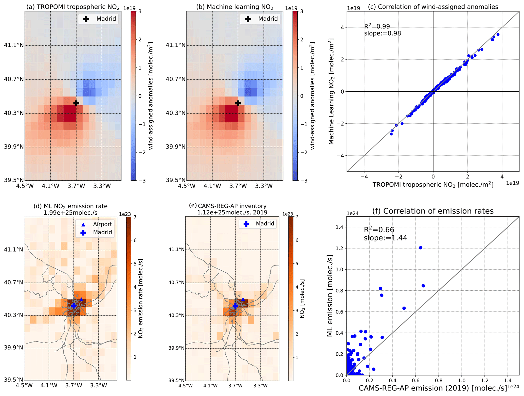
Figure 2 Panels (a)–(d) show the same information as Fig. 1a–d, respectively, but for the Madrid area in Spain. Panel (e) presents the spatial distribution of the CAMS-REG-AP inventory in 2019, and panel (f) shows the correlation of emission rates between ML and the CAMS-REG-AP inventory.

3.3 NO₂ emission changes on weekdays and at weekends

NO_x emission variations result in significant changes in the weekly cycle, which is an unequivocal sign of anthropogenic sources (Beirle et al., 2003).

The estimated emission rates for weekdays (Sunday to Thursday) and weekends (Friday and Saturday) in Riyadh are presented in Fig. 3. It should be noted that the weekends in Saudi Arabia are Fridays and Saturdays. The lowest NO₂ column abundances are observed on Fridays, followed by those on Saturdays (Fig. A7). The NO₂ emissions were reduced by 16 % at weekends, and high reductions were found near the city center and the areas along Highway 65. Highway 65 is a major north–south highway in central Saudi Arabia and runs in the southeast–northwest direction, connecting Riyadh to Al Majma'ah in the northwest and to Kharj in the southeast (Fig. A8).

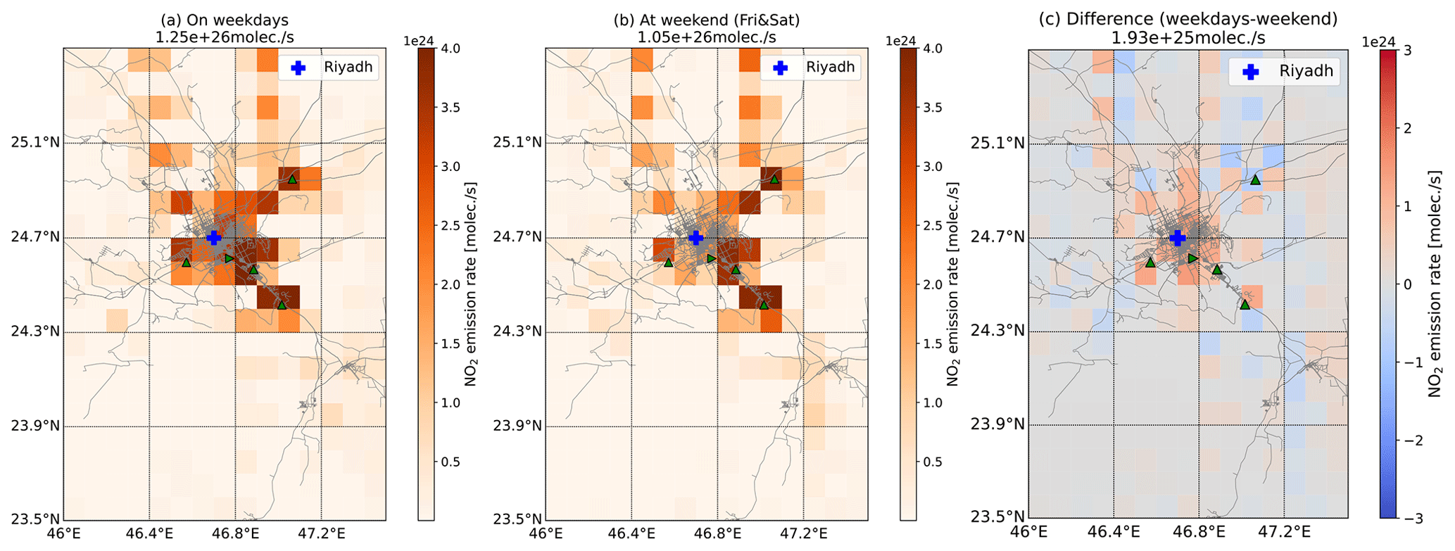
Figure 3 Averaged ML-estimated emission strengths for (a) weekdays (Sunday to Thursday), (b) weekends (Friday and Saturday), and (c) their difference (weekdays − weekend) in Riyadh. The number in each panel heading presents the total emission rate.

Significant column declines are found in large cities, especially in Europe, at weekends (Stavrakou et al., 2020). The weekly cycle of NO₂ column abundances in the Madrid area is different from that in Riyadh, as the lowest amounts are observed on Sundays, the second day of the weekend (Fig. A9). An outstanding difference becomes apparent: much higher NO₂ amounts are found on workdays, especially in urban areas. These high emissions are mainly due to road transport, which is the largest NO_x contributor in Europe (Crippa et al., 2018) and emits up to 90 % of the NO₂ in Madrid (Borge et al., 2014).

The ML-estimated emission strengths for Madrid are presented in Fig. 4. High NO₂ emission sources on weekdays are evenly distributed around the city center (Fig. 4a). However, at weekends, the northeastern regions close to the airport, far from the city center, are the main sources, and no obvious sources are observed in the southwestern regions (Fig. 4b). The total NO₂ emission strength in the urban area (denoted using dashed rectangles) at weekends (7.62×10²⁴ molec. s⁻¹) is about 28 % lower than that observed on weekdays (1.06×10²⁵ molec. s⁻¹). This result is similar to the result observed in another European city – Helsinki, where the weekly variability in traffic-related emissions was reduced by 30 % at weekends (Ialongo et al., 2020). By subtracting weekend emissions from those on weekdays (Fig. 4c), we found that the dominant NO₂ sources are in the east-to-northeast and south-to-southwest regions, where the residential areas and workplaces are mainly located (Fig. A10). Orographic features further cause the accumulation of NO₂ in these regions (see Sect. 3.2). The wind-assigned anomalies and correlation plots are presented in Fig. A11. Note that slightly higher scattering in the results at weekends is mostly due to fewer data points.

Figure 4 The same as Fig. 3 but for the Madrid area. The number in each panel heading presents the total emission rate in the dashed rectangle (70×70 km²).

3.4 COVID-19 lockdown effect

The current global pandemic caused by the coronavirus disease (COVID-19) has largely impacted human life and the economic situation. To minimize the spread of the COVID-19 (SARS-CoV-2) virus, countries around the world have enforced lockdown measures. Recent studies have reported decreasing NO_x concentrations in the atmosphere due to lockdown measures as well as additional reductions in areas with more stringent lockdown measures, such as in Spain (Abdelsattar et al., 2021; Barré et al., 2021; Sun et al., 2021; Liu et al., 2021; Vîrghileanu et al., 2020; Keller et al., 2021; Bauwens et al., 2020; Fan et al., 2020; Huang and Sun, 2020). An approximate 40 % decrease in NO₂ was observed in Riyadh by OMI (Abdelsattar et al., 2021). Bauwens et al. (2020) illustrated the impact of the COVID-19 outbreak on NO₂ based on TROPOMI and OMI observations. The averaged NO₂ column decreased by ∼29 % as derived from TROPOMI observations and by ∼21 % as derived from OMI observations in Madrid during the lockdown period (Bauwens et al., 2020). These NO₂ reductions are strongly related to the lockdown policy and are also presented in the study by Levelt et al. (2022), who reported that NO₂ column amounts decreased by 14 %–63 % in megacities globally. A sharp reduction of 54 % in the NO₂ tropospheric column amounts was observed in Madrid during the lockdown period, and a reduction of 36 % was noted during the transition period. The time series of TROPOMI tropospheric NO₂ columns displays an obvious decrease when the lockdown started in early 2020 (Fig. A12). The NO₂ amounts reached their lowest values in April 2020; since this time, they have gradually returned to normal levels, as in previous years. We analyze the same seasonal period in 2019 (before lockdown, March–June 2019) and in 2020 (during the lockdown, March–June 2020) for Riyadh and Madrid.

Figure 5 presents the spatial distribution of estimates before and during the lockdown in Riyadh. NO₂ emissions decreased by 21 %: from 1.23×10²⁶ molec. s⁻¹ before lockdown to 9.67×10²⁵ molec. s⁻¹ during lockdown. The spatial distribution of estimates during lockdown is similar to that at weekends, when significant decreases are observed along Highway 65 and emissions are generally reduced in the city center and in the areas where the cement plant and power plants are located.

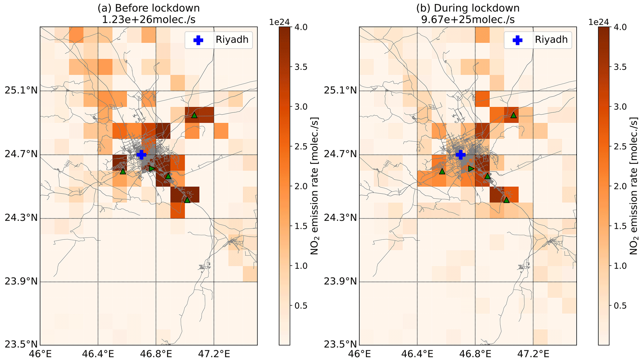
Figure 5 Averaged ML-estimated emission strengths before lockdown (March–June 2019) and during lockdown (March–June 2020). The number in each panel heading presents the total emission rate.

The NO₂ emission estimate in the urban area of Madrid is about 1.14×10²⁵ molec. s⁻¹ before lockdown, and it decreases by 62 % to 4.30×10²⁴ molec. s⁻¹ during the lockdown period (Fig. 6). This result fits well with recent studies (Baldasano, 2020; Barré et al., 2021; Guevara et al., 2021). The European Environment Agency (EEA) also reported a 56 %–72 % reduction in NO₂ concentrations in Madrid based on in situ monitoring data (EEA, 2020). Even compared with the emission at weekends, the lockdown emission was reduced by 44 %. The regions with high NO₂ emissions are constrained to the east of Madrid, where there are residential areas. Note that the lockdown spatial pattern reproduces the pattern observed at weekends during the whole period (Fig. 4b), corroborating that NO₂ emissions are highly related to transportation. Civil aviation was also restricted during the lockdown and, thus, a lower NO₂ emission strength is observed close to the airport. The reduction in Madrid was larger than that in Riyadh, as Madrid was under a very strict lockdown policy.

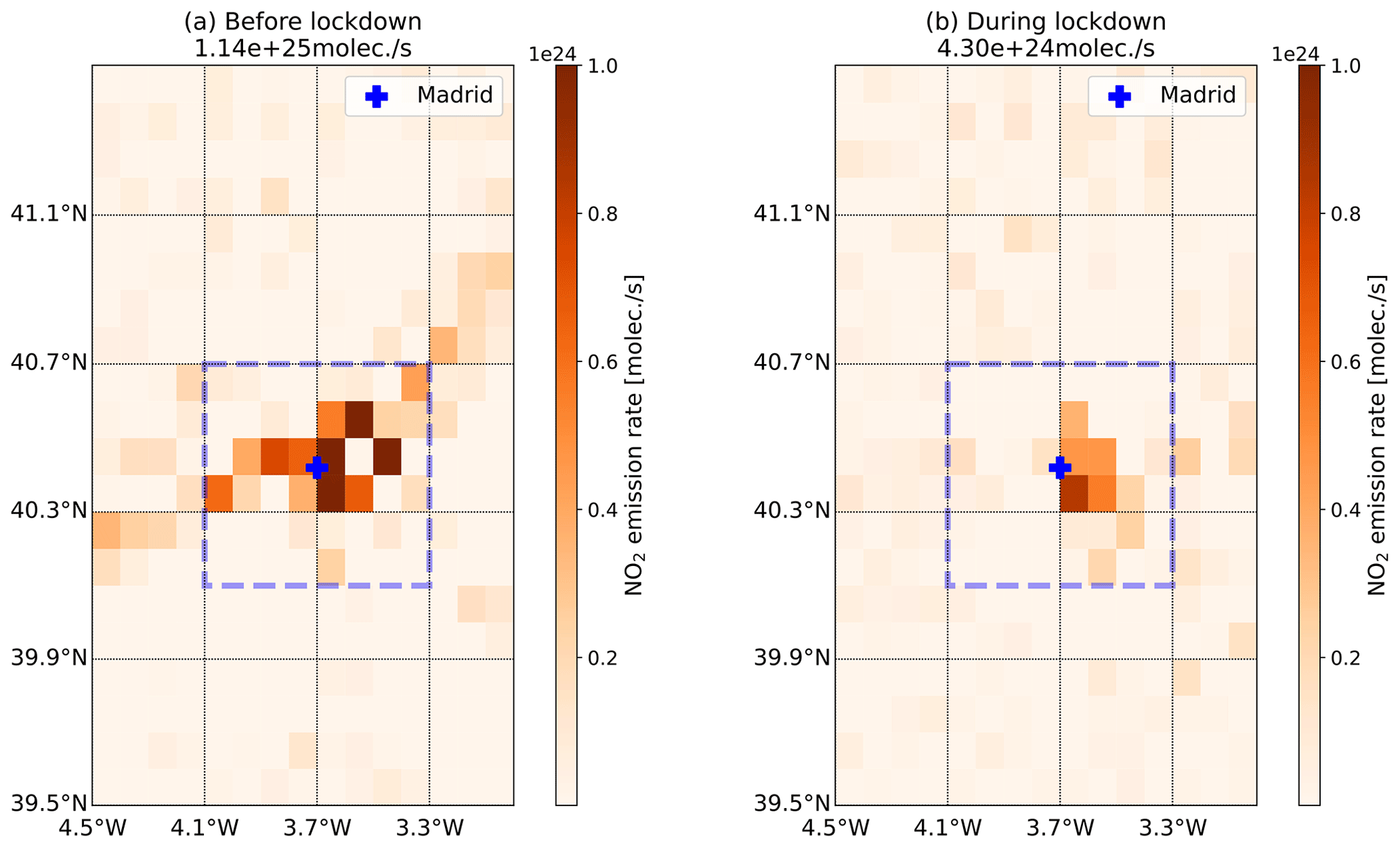
Figure 6 The same as Fig. 5 but for the Madrid area. The number in each panel heading presents the total emission rate in the dashed rectangle (70×70 km²).

4 Uncertainty analysis

4.1 Different choice of α and τ values

The angle (α) of the emission cone is an empirical value, as is the lifetime/decay time (τ) for NO₂. These values can introduce uncertainties; thus, different α and τ values are used to investigate their impacts on emissions. The spatial patterns of the estimates using different α or τ values are quite similar. The absolute values of the emission rate increase with increasing α (see Fig. 7a). A change of 10^∘ in α introduces a difference of less than 3.2 %. A decrease of 1.5 % is observed when using $\mathit{\alpha }=\mathrm{50}{}^{\circ }$, and an increase of 1.4 % is observed for $\mathit{\alpha }=\mathrm{70}{}^{\circ }$, compared with $\mathit{\alpha }=\mathrm{60}{}^{\circ }$. Increasing values of τ result in lower estimates (see Fig. 7b). With respect to the result obtained with τ= 4 h, the estimate increases by ∼42 % for τ=3 h and decreases by ∼20 % for τ=5 h.

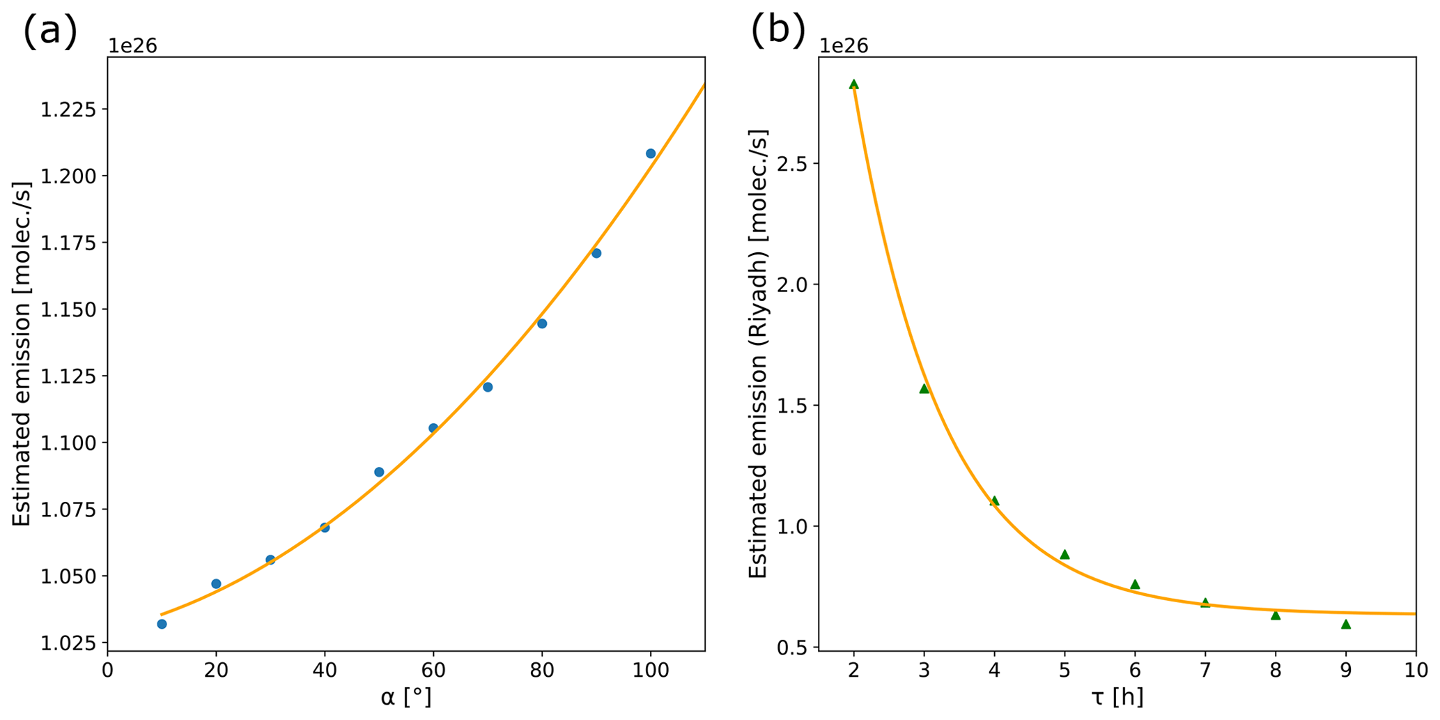
Figure 7 Estimated emissions using a different cone angle α (a) and NO₂ lifetime τ (b) based on TROPOMI data in Riyadh in 2019.

4.2 Different choice of wind field segmentation

The wind field segmentation is decided based on the predominant wind fields. We chose different segmentation for Riyadh (i.e., SW comprised 135–315^∘ and NE comprised the rest of the fields) and for Madrid (i.e., SE comprised 45–225^∘ and NW comprised the rest of the fields). The spatial pattern of the estimates in Riyadh (Fig. 8a) is similar to previous results, whereas some unexpected positive emissions are obtained southwest of Madrid. Increases of 11.0 % in Riyadh and 4.5 % in Madrid are estimated. Using different wind segmentation leads to different spatial distributions of estimates, especially in Madrid where the topography (e.g., land cover, altitude) is more complicated than in Riyadh.

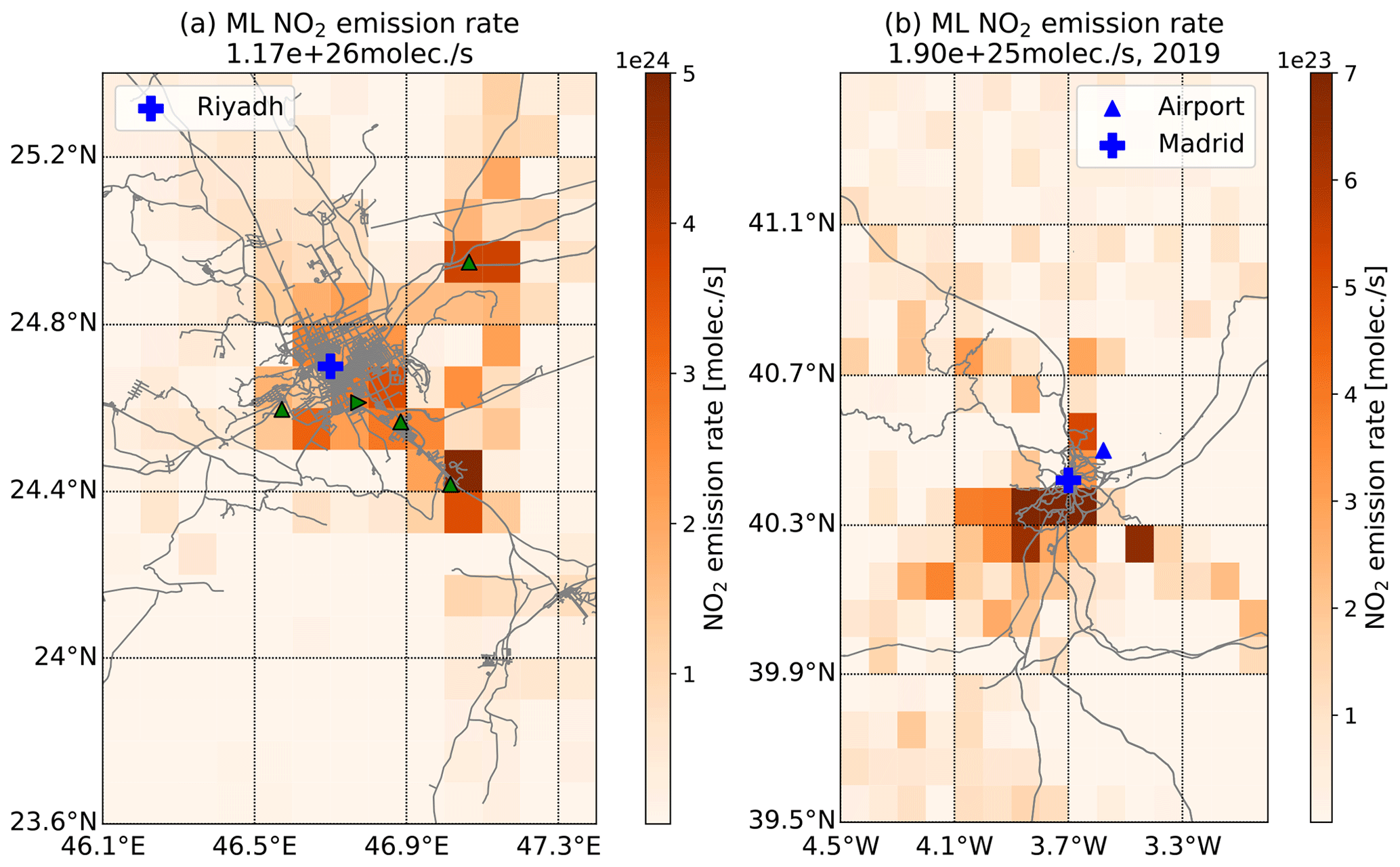
Figure 8 Panel (a) is similar to Fig. 1d but using southwest–northeast wind field segmentation; panel (b) is similar to Fig. 2d but using southeast–northwest wind field segmentation. Note that data are based on TROPOMI data in 2019.

4.3 Different choice of wind field in the vertical and horizontal dimensions

The wind speed increases with altitude (Fig. A2c, f), whereas the distribution of the wind directions remains similar. Approximate increases of 19 % and 39 % in the wind speed at 100 m are observed in Riyadh and Madrid, respectively. The estimates change slightly in both cities, as the wind-assigned method compensates for the increases in both wind fields.

To limit the computational effort, we simplified the horizontal distribution of the wind field to an even distribution, i.e., constant wind speed and wind direction over the study area at each time gap (1 h). This might introduce some errors; thus, a full year of data in 2020 is used to investigate the uncertainty. The wind direction and speed are interpolated at each pixel center, as ERA5 wind is at a spatial resolution of $\mathrm{0.25}{}^{\circ }\times \mathrm{0.25}{}^{\circ }$. Either the spatial distribution or the estimated emission is similar to those with a constant wind field in both cities. The estimates change by 1.9 % in Riyadh and by −1.3 % in Madrid. The average pixel-to-pixel difference is 6.8×10²¹ ($\pm \mathrm{4.6}\times {\mathrm{10}}^{\mathrm{23}}$) molec. s⁻¹ in Riyadh and $-\mathrm{8.3}\times {\mathrm{10}}^{\mathrm{20}}$ ($\pm \mathrm{4.5}\times {\mathrm{10}}^{\mathrm{22}}$) molec. s⁻¹ in Madrid.

Figure 9 Panels (a) and (b) are similar to Figs. A4c and A5c, respectively, but using a spatially varying wind field.

5 Conclusions

This paper proposes a combination of wind-assigned anomalies and machine learning (ML) methods to estimate the average tropospheric NO₂ emission strength and its spatial pattern derived from TROPOMI observations from May 2018 to June 2022. The Adaptive Moment Estimation (ADAM) algorithm, as one of the gradient descent ML algorithms, is chosen because of its high efficiency and low cost requirements.

Riyadh is first used as a test site due to its high population density, remote location with respect to other sources, and favorable weather conditions, which allow for the high availability of space-based observations. Consistent wind-assigned plumes are found based on TROPOMI measurements and on the ML-trained plumes. A very good correlation is obtained between these two wind-assigned plumes, with an R² value of 1.0 and a slope of 0.99. The spatial pattern of the estimated emission strengths of the main sources near the city center also agrees with the results from Beirle et al. (2019). Several NO₂ emission hotspots, associated with a cement plant and power plants, are discernible. The total emission rate over the whole area is about 1.09×10²⁶ molec. s⁻¹, which is higher than the aforementioned previous study (8.5×10²⁵ molec. s⁻¹; Beirle et al., 2019). This difference might be due to the different study period and methods. These results suggest that our combined method works properly and is reliable.

We extended this method to the (mega)city of Madrid, Spain. The averaged NO₂ emission estimates are 1.99×10²⁵ molec. s⁻¹ in total, and the dominant emitting area is around the city center, especially in the north-to-northeast and south-to-southeast regions. The region including the international Madrid-Barajas Airport in the northeast is also distinguished by high emission rates, as aircraft exhaust emissions are highly enriched in NO₂ during taxi and takeoff (Herndon et al., 2004). The orographic features also cause NO₂ accumulation in the northeast–southwest regions, along the Guadarrama mountain range.

NO₂ emission is highly related to transportation; thus, NO₂ emission changes between weekdays and weekends are investigated as well. Different weekly cycles of NO₂ are observed in Riyadh and Madrid. In Riyadh, the lowest NO₂ column abundances are observed on Fridays, followed by those on Saturdays. Moreover, NO₂ emissions are reduced by 16 % at weekends, and high reductions are found near the city center and the areas along Highway 65. In Madrid, the regions to the west and southwest of the city are not the main NO₂-emitting areas at weekends, but they are main source areas on weekdays, indicating that many workplaces are located in the southwest. The estimates are 1.06×10²⁵ molec. s⁻¹ on weekdays and 7.62×10²⁴ molec. s⁻¹ at weekends in the urban area (70 km × 70 km²). This 28 % reduction in NO₂ emissions is mainly due to people commuting from home to the city center and workplaces.

Many studies have demonstrated that the lockdown policy response to the COVID-19 pandemic reduced NO₂ emissions (Barré et al., 2021; Sun et al., 2021; Liu et al., 2021; Vîrghileanu et al., 2020; Keller et al., 2021; Bauwens et al., 2020; Fan et al., 2020; Huang and Sun, 2020). Countries like Spain imposed a very stringent lockdown beginning in March 2020. An average NO₂ emission reduction of 62 % was observed during the lockdown (March–June 2020) compared with the March–June 2019 period. The regions with dominant NO₂ emissions during lockdown were limited to the east of Madrid, where there are residential areas. Reduced NO₂ emissions (21 %) were observed in Riyadh, especially near the city center. This reduction was much smaller than that in Madrid, as the latter was under a very strict lockdown regulation.

Our easy-to-apply method has successfully proven its consistency and reliability using two contrasting examples (Riyadh and Madrid). However, its application in some areas with a complicated emission source distribution and topography might not be feasible. The varying decay time for short-lived species in different regions and seasons is another important factor affecting the estimates of emissions. We plan to include these refinements in future studies in order to reduce the uncertainties in both the wind-assigned anomaly method and the ML approach. The spatial distributions of estimates generally show checkerboard-like structures. We assume that these structures indicate that the inversion attempts to resolve fine structures that are poorly constrained by the observations. When we converge to a stable solution with minimal bias, we are confident that the spatially averaged retrieved emissions are more realistic. It is our hope that the method presented here can be applied to other key gases, such as carbon dioxide or methane, for which the background concentration needs to be considered as well as to other regions. Meanwhile, the powerful ML framework might allow one to investigate related questions – for example, perhaps a joint estimation of the NO₂ lifetime and the emission strength would be possible.

Appendix A

Figure A1 The number of TROPOMI measurements in each 0.1^∘ grid pixel for Riyadh and Madrid during May 2018–June 2022.

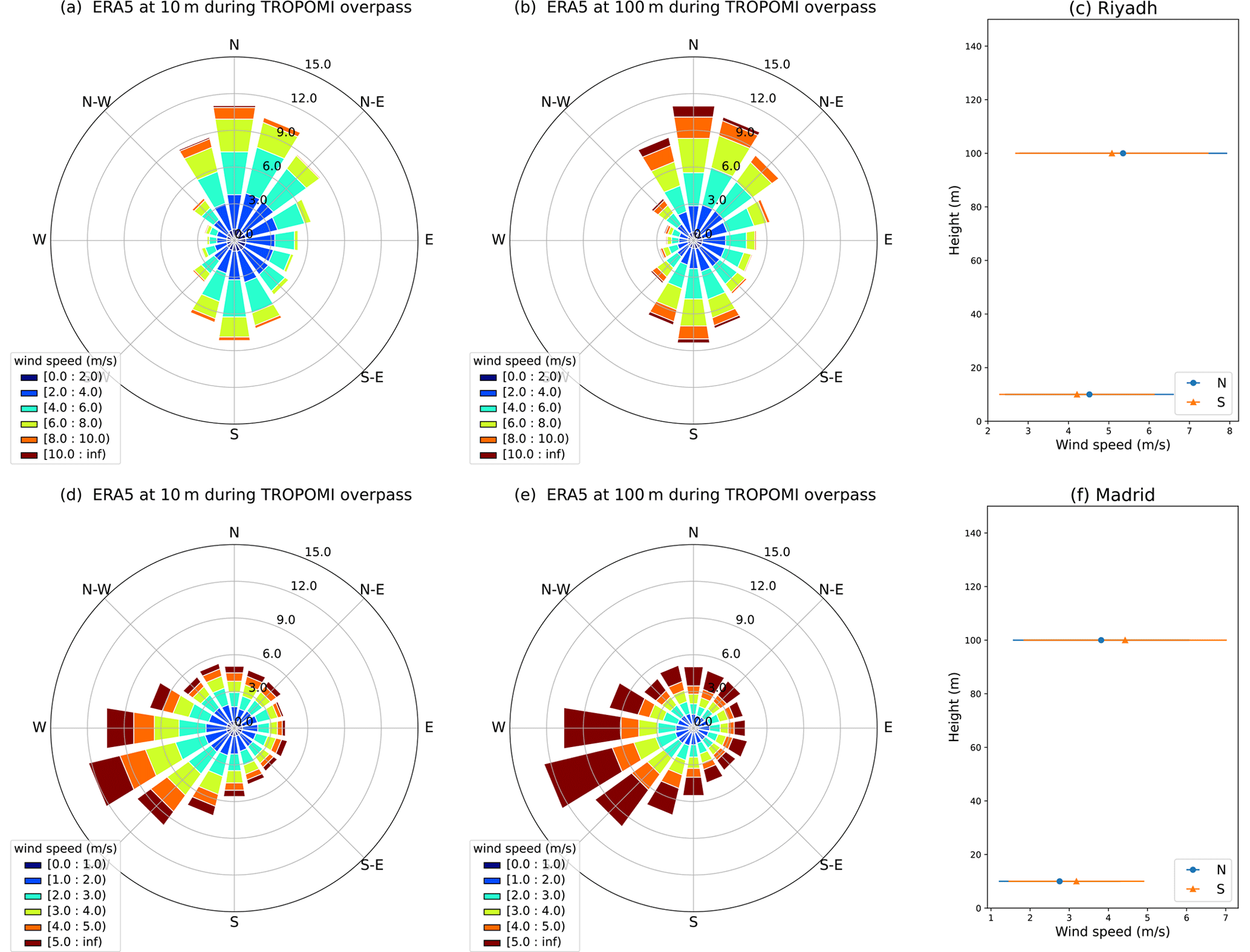
Figure A2 Wind roses of the daytime ERA5 model wind at 10 and 100 m during TROPOMI overpasses and of wind speed at two levels in Riyadh (a–c) and Madrid (d–f).

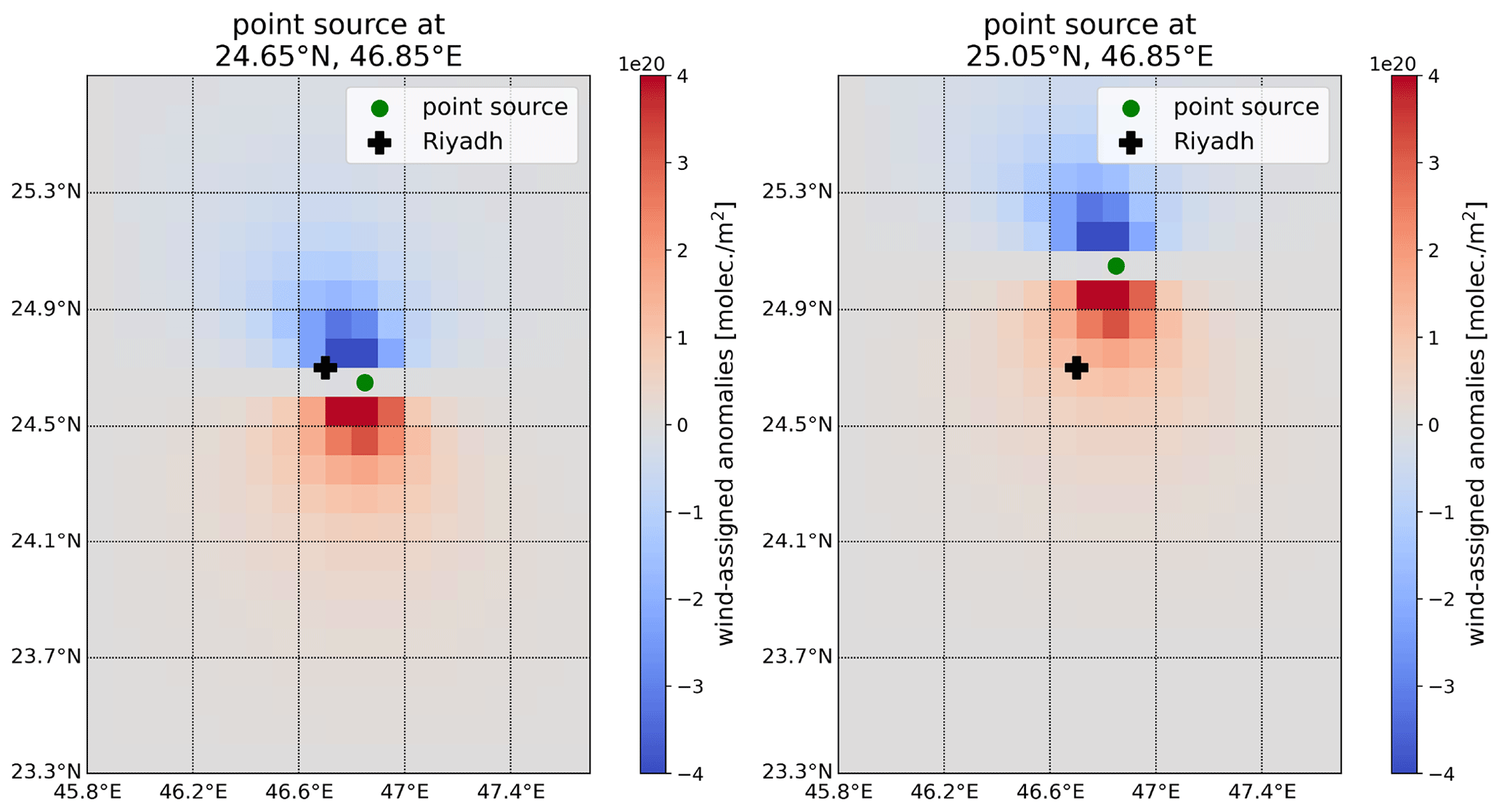
Figure A3 Examples of a wind-assigned plume for the point sources at 24.65^∘ N, 46.85^∘ E and at 25.05^∘ N, 46.85^∘ E in Riyadh.

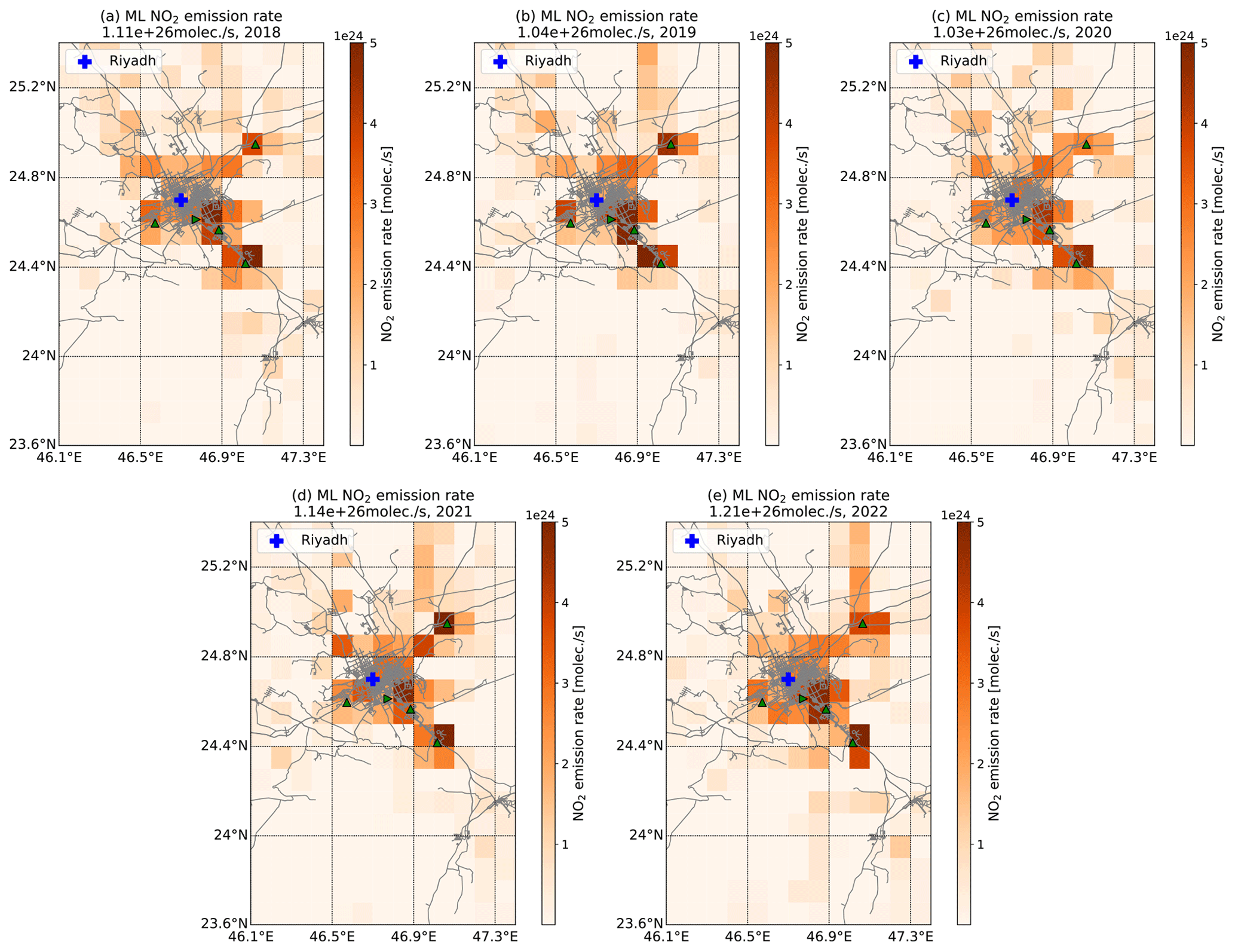
Figure A4 Yearly averaged estimated NO₂ emission rates in Riyadh for the years 2018 to 2022. Note that data in 2018 started from May and data in 2022 ended in June.

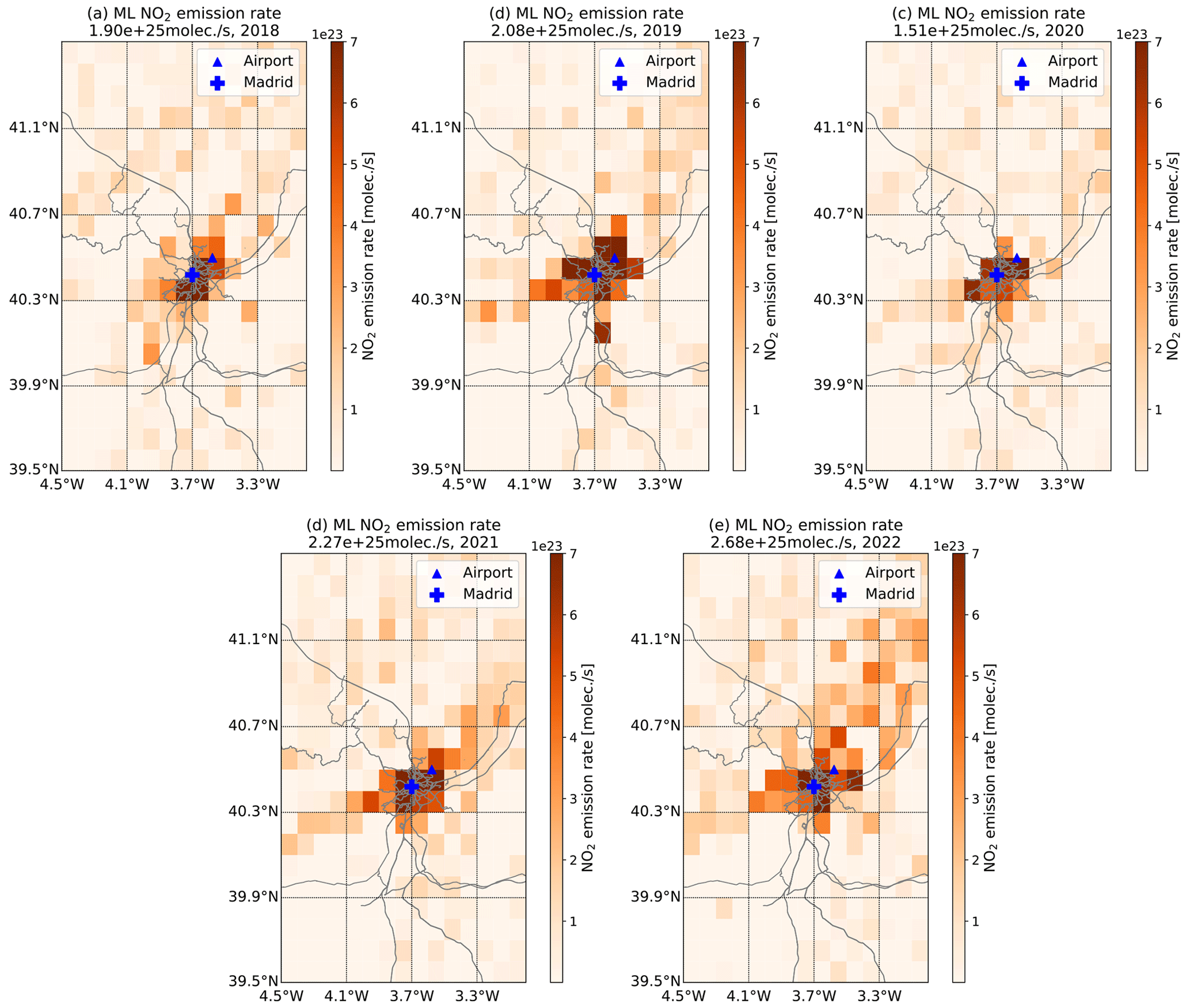
Figure A5 Similar to Fig. A4 but for the Madrid area.

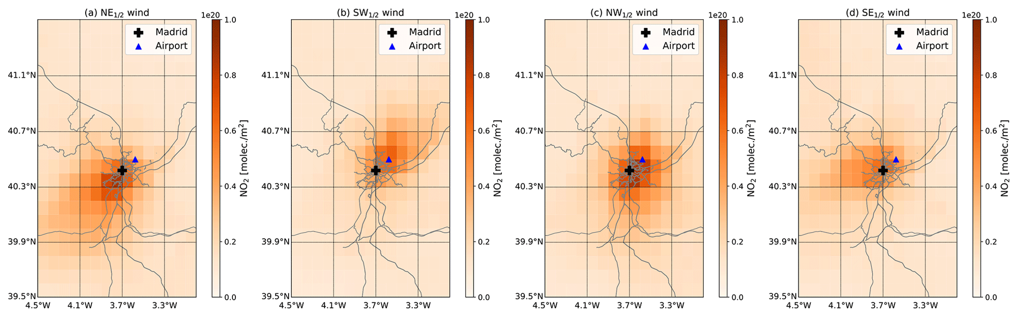
Figure A6 TROPOMI tropospheric NO₂ column for narrow wind regimes covering (a) NE${}_{\mathrm{1}/\mathrm{2}}$ (0–90^∘), (b) SW${}_{\mathrm{1}/\mathrm{2}}$ (180–270^∘), (c) NW${}_{\mathrm{1}/\mathrm{2}}$ (270–360^∘), and (d) SE${}_{\mathrm{1}/\mathrm{2}}$ (90–180^∘), respectively.

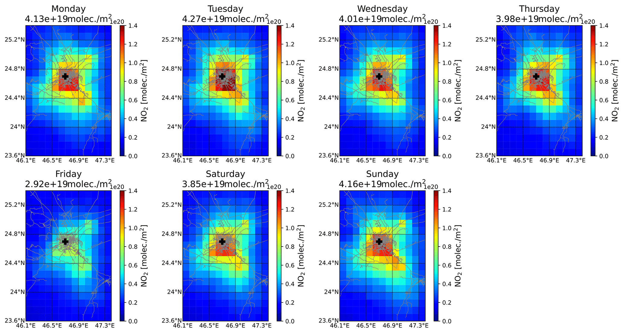
Figure A7 The TROPOMI tropospheric NO₂ column during the week in Riyadh. The number in the panel heading represents the average column abundance over the area.

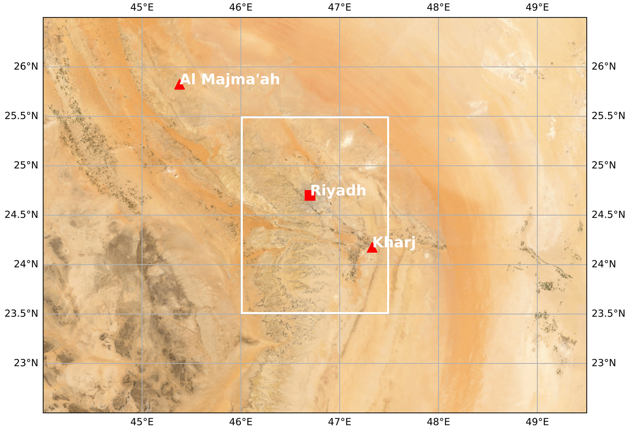
Figure A8 Map of Riyadh (© Esri). The area in the white rectangle represents the study area.

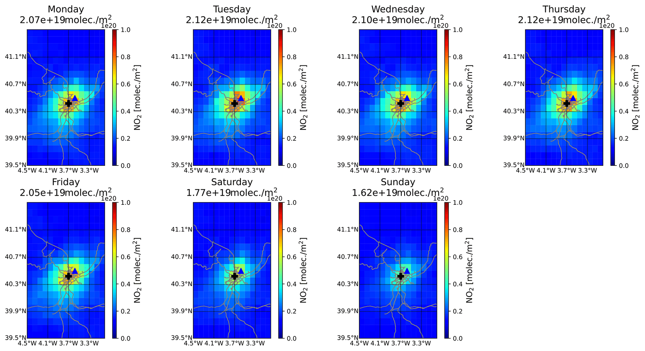
Figure A9 The same as Fig. A7 but for the Madrid area.

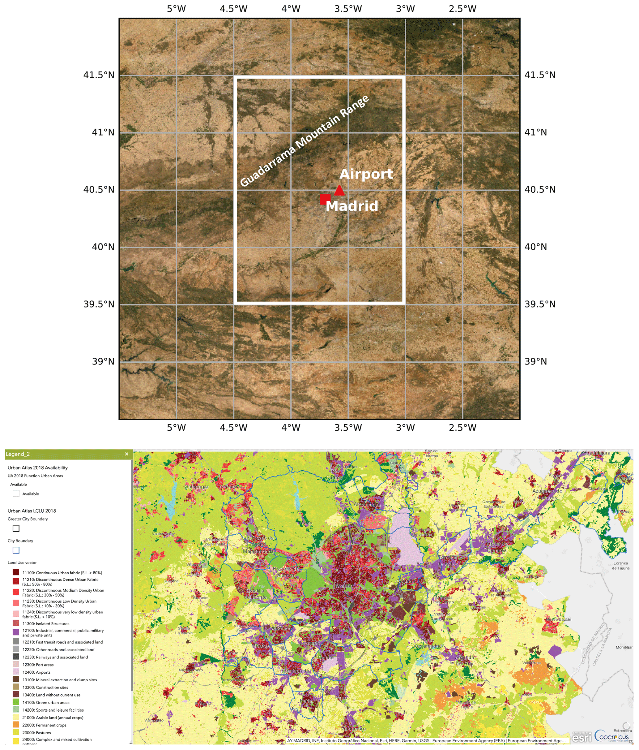
Figure A10 Map of the study area (top; © Esri) and a zoomed-in version (bottom; https://land.copernicus.eu/local/urban-atlas/urban-atlas-2018, last access: 25 April 2022) for Madrid.

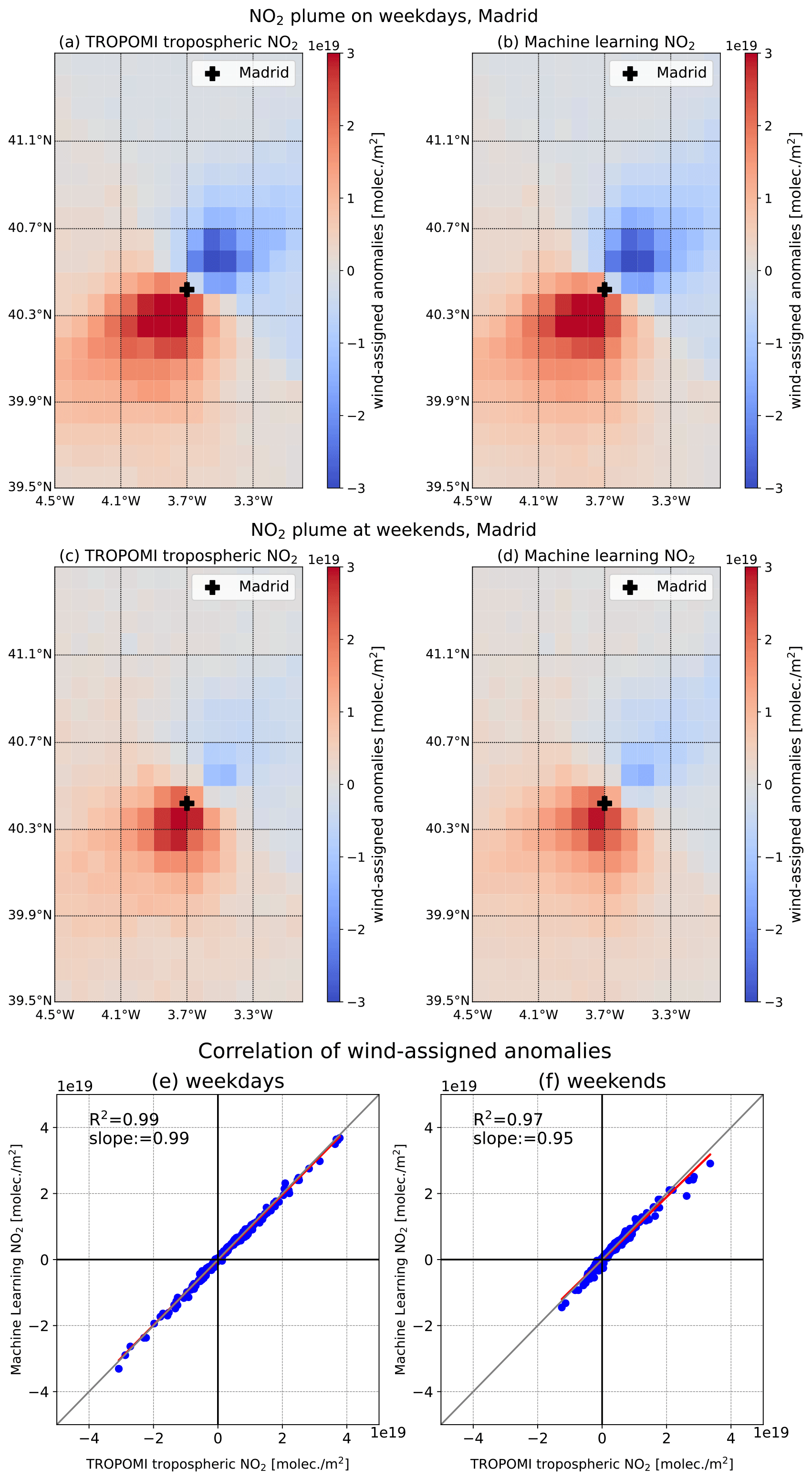
Figure A11 Wind-assigned plumes derived from TROPOMI observations (a, c), the ML method (b, d), and their correlation plots (e, f) on weekdays (a, b, e) and weekends (c, d, f) in Madrid.

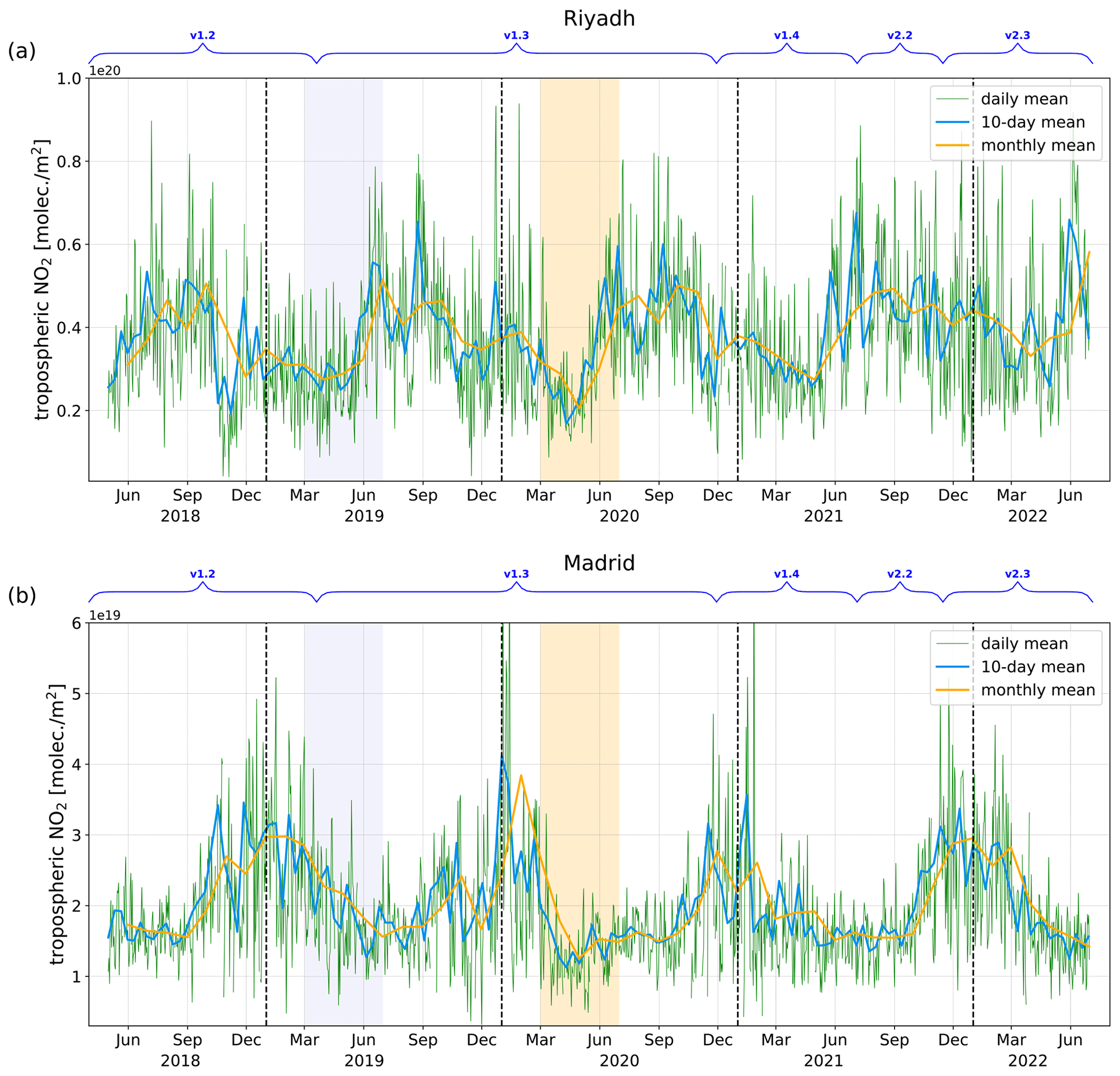
Figure A12 Time series of TROPOMI tropospheric NO₂ columns in terms of the daily, 10 d, and monthly mean in (a) Riyadh and (b) Madrid. The areas marked using lavender and orange colors are the study periods in 2019 and 2020, respectively. The annotations on top of each panel represent the different versions of data sets.

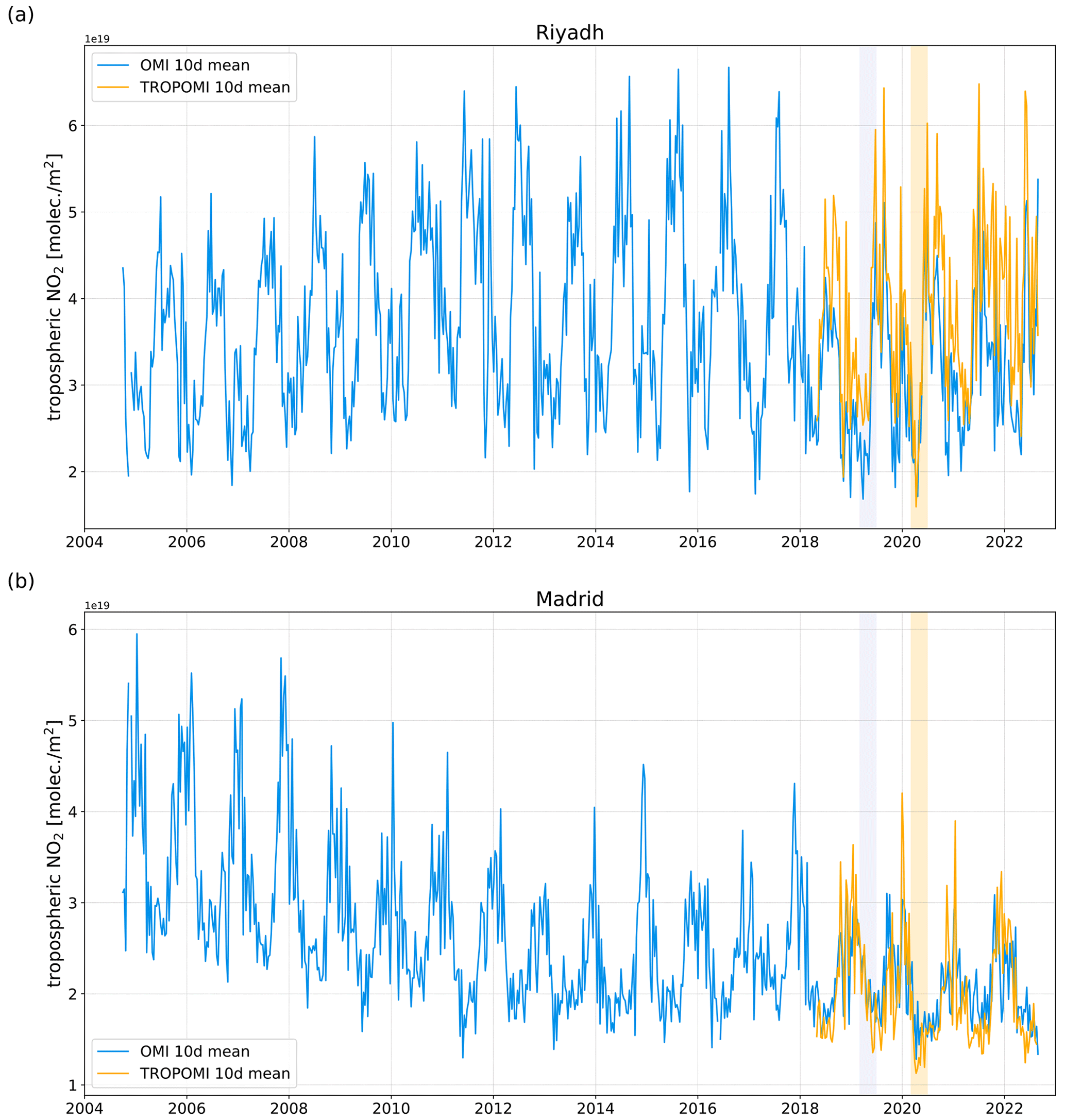
Figure A13 Time series of the TROPOMI and OMI tropospheric NO₂ columns in terms of the 10 d mean in (a) Riyadh and (b) Madrid. The areas marked using lavender and orange colors are the study periods in 2019 and 2020, respectively

Figure A14 Correlation plot between the TROPOMI and OMI tropospheric NO₂ columns.

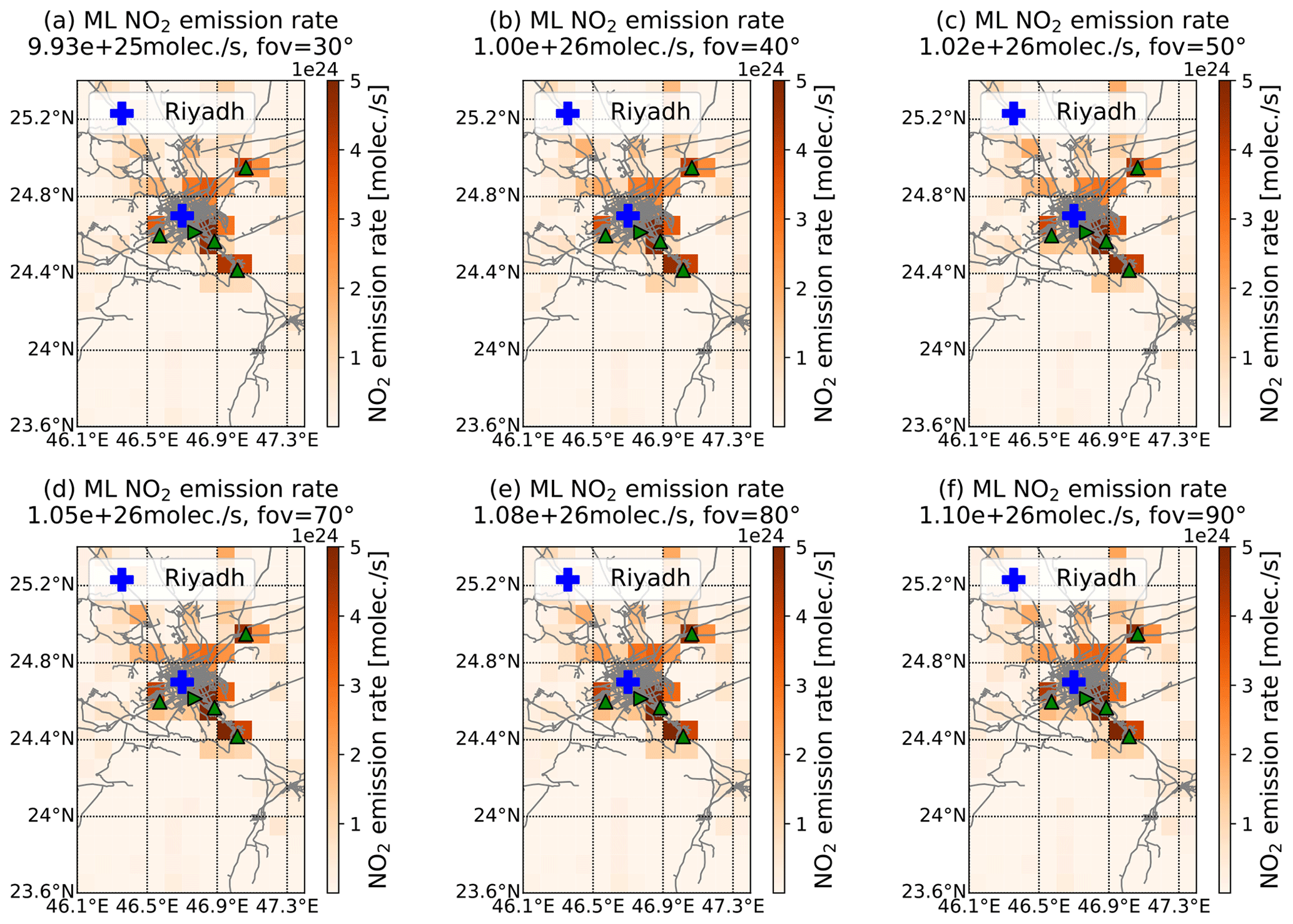
Figure A15 Estimated emission rates in Riyadh for different angles (α) of the emission cone from 30 to 90^∘.

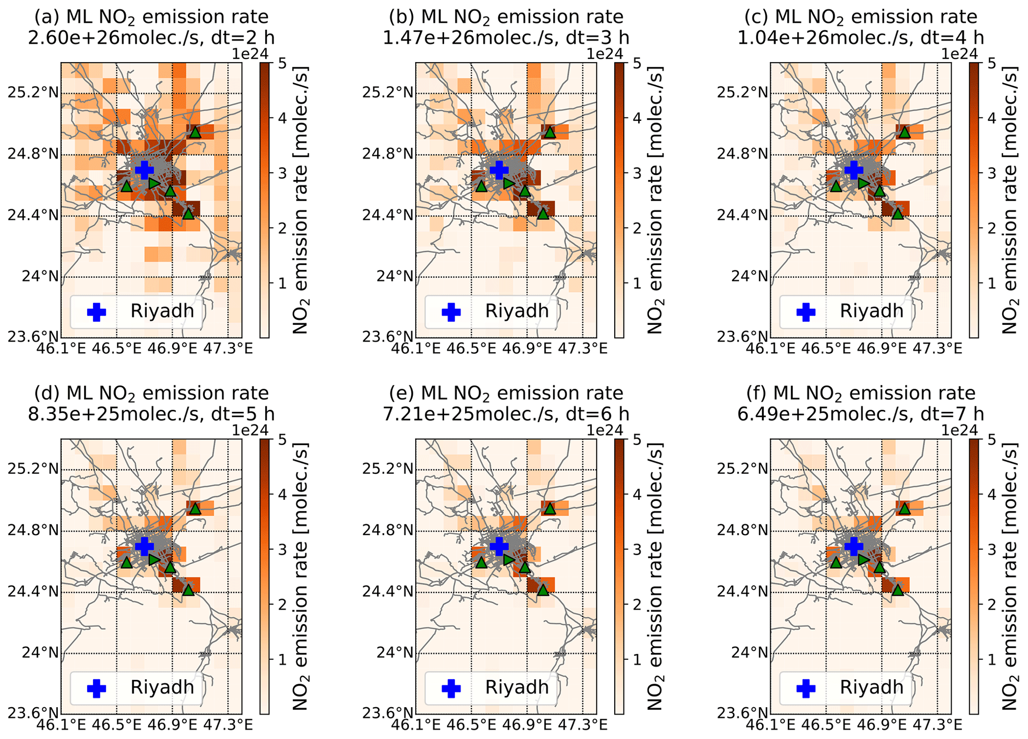
Figure A16 Estimated emission rates in Riyadh for a different decay time (τ) from 1 to 7 h. Note that the color bars are different from that in Fig. 1d in order to cover a larger range.