Across-track extension of retrieved cloud and aerosol properties for the EarthCARE mission: the ACMB-3D product

The narrow cross section of cloud and aerosol properties retrieved by L2 algorithms that operate on data from EarthCARE's nadir-pointing sensors is broadened across-track by an algorithm that is described and demonstrated here. This scene construction algorithm (SCA) consists of four components. At its core is a radiance-matching procedure that works with measurements made by EarthCARE's Multi-Spectral Imager (MSI). In essence, an off-nadir pixel gets filled with retrieved profiles that are associated with a (nearby) nadir pixel whose MSI radiances best match those of the off-nadir pixel. The SCA constructs a 3D array of cloud and aerosol (and surface) properties for entire frames that measure ∼6000 km along-track by 150 km across-track (i.e., the MSI's full swath). Constructed domains out to ∼15 km across-track on both sides of nadir are used explicitly downstream as input for 3D radiative transfer models that predict top-of-atmosphere (TOA) broadband solar and thermal fluxes and radiances. These quantities are compared to commensurate measurements made by EarthCARE's Broadband Radiometer (BBR), thus facilitating a continuous closure assessment of the retrievals. Three 6000 km ×200 km frames of synthetic EarthCARE observations were used to demonstrate the SCA. The main conclusion is that errors in modelled TOA fluxes that stem from use of 3D domains produced by the SCA are expected to be less than ±5 W m⁻² and rarely larger than ±10 W m⁻². As such, the SCA, as purveyor of information needed to run 3D radiative transfer models, should help more than hinder the radiative closure assessment of EarthCARE's L2 retrievals.

1 Introduction

The objective of the EarthCARE satellite mission is to help improve numerical predictions of weather, air quality, and climatic change via application of synergistic L2-retrieval algorithms to observational data from its cloud-profiling radar (CPR), backscattering lidar (ATLID), and passive multi-spectral imager (MSI) (Illingworth et al., 2015). EarthCARE's overarching scientific goal (ESA, 2001) is to retrieve cloud and aerosol properties with enough accuracy that when used to initialize atmospheric radiative transfer (RT) models, simulated top-of-atmosphere (TOA) broadband radiative fluxes, for domains covering ∼ 100 km², agree with their observation-based counterparts to within ±10 W m⁻² more often than not. Observed TOA fluxes derive from radiances measured by EarthCARE's multi-angle broadband radiometer (BBR). As the latter are not used by retrieval algorithms, comparing them to modelled values, obtained by RT models operating on retrieved quantities, affects a moderately stringent verification of the retrievals (Barker et al., 2023) – moderately stringent because BBR radiances consist, in part, of photons that share the same gaseous pathlength and number of cloud–aerosol–surface scattering event distributions as those that constitute MSI radiances. These imperfections aside, this radiative closure verification is a well-defined and cost-effective final stage in EarthCARE's formal processing chain (Eisinger et al., 2023).

In light of EarthCARE's ambitious goal of limiting differences between measured and modelled TOA fluxes to ±10 W m⁻² when averaged over assessment domains that measure ∼ 5 km across-track by ∼ 21 km along-track, the usefulness of its radiative closure programme depends much on reducing errors and uncertainties in BBR measurements, variables needed by RT models that are not provided by EarthCARE observations, and RT models. Included in this are issues of observational geometry that face use of BBR data for EarthCARE's closure assessment. First, L2-retrieved profiles are ∼ 1 km in diameter, while the BBR was designed to perform best for footprints of ∼ 10 × 10 km. For this configuration, fluxes and radiances computed for sequences of retrieved profiles contribute only ∼ 10 % of the signal to each BBR footprint (or pixel). Second, at only ∼ 1 km wide, net horizontal fluxes for each retrieved column and sequences of them will rarely be close to zero (e.g., Barker and Li, 1997; Marshak et al., 1998). This implies that 3D RT models, as opposed to their ubiquitous 1D counterparts, will be required to make EarthCARE's radiative closure assessment fruitful (Illingworth et al., 2015) – hence the need for 3D arrays of data that describe the Earth–atmosphere system adjacent to the ∼ 1 km wide retrieved L2 cross section.

Fortunately, BBR data are not bound to 10 km resolution, as point-spread function widths of its native radiances are ∼ 0.7 km. This offers much flexibility to the design of the closure assessment (e.g., Tornow et al., 2015). The extreme case is to use a single along-track line of BBR radiances that overlap, at best approximately, the ∼ 1 km wide curtain of L2-retrieved profiles, referred to hereinafter as the L2 plane. This would, however, degrade BBR performance, via reduced signal-to-noise ratio and pointing accuracy, and thus weaken closure assessments. Alternatively, one could attempt an across-track broadening of the L2 plane so as to cover as many BBR native radiances as deemed necessary. Regardless of the route taken and the size of domains over which closure assessments are to be performed, there is the ever-present related issue of lateral flow of photons both within assessment domains and between assessment domains and their adjacent areas. Taking these issues together, EarthCARE's science team opted for its closure assessment experiment to use 3D RT models applied to assessment domains centred on the L2 plane with across-track widths appreciably greater than 1 km (Illingworth et al., 2015).

The method for approximating 3D geophysical variables adjacent to the L2 plane, in order to safely use both 3D RT models and BBR data, is the radiance-matching scene construction algorithm (SCA) (Barker et al. 2011), which forms the basis of the ACMB-3D processor. The purpose of the current paper is to recap, in Sect. 2, the SCA; present several operational details associated with it; and demonstrate, in Sect. 3, its overall performance using simulated observations for a virtual Earth–observation system (Qu et al. 2023; Donovan et al. 2023). The application of RT models to SCA products and subsequent radiative closure assessments for the same virtual environments are discussed by Cole et al. (2023) and Barker et al. (2023). A brief discussion is given in Sect. 4.

2 Three-dimensional atmosphere–surface scene construction algorithm

To begin, EarthCARE's products are partitioned into ∼5000 km long frames, which makes eight​​​​​​​ frames/orbit. Position in a frame is defined by the Joint Standard Grid (JSG). Each frame contains N_JSG L2-retrieved columns along-track. Frame widths are 150 km as defined by the Multi-Spectral Imager's (MSI) swath: 35 km to the right and 115 km to the left of the L2 plane (relative to the satellite's direction of motion). Some algorithms require data beyond nadir, and so each frame's files also contain n_ε swaths of data from neighbouring frames. JSG coordinates are denoted as (i,j), with i running along-track from 1−n_ε to N_JSG+n_ε and j running perpendicular to the L2 plane, which is located at j=0.

As documented by Cole et al. (2022), EarthCARE's radiative products are produced by 1D and 3D broadband RT models. Some of these products are used to perform radiative closure assessments of L2 retrievals (see Barker et al., 2023). While 1D RT models are applied, in ACM-RT (see Cole et al., 2022), to all non-corrupt columns in the L2 plane, their results are averaged over small domains D in processor ACMB-DF, where radiative closure is assessed, referred to hereinafter as assessment domains, whose along-track centres, at j=0, are the L2 plane. Conversely, 3D RT models operate directly on D, and domain-average results are computed in ACM-RT and used in ACMB-DF. The structure of D for j≠0 is defined by the 3D scene construction algorithm (SCA), which is explained in the following subsections. Along-track lengths of D, in terms of JSG cells, are n_assess columns (pixels), while their across-track half-widths are m_assess, making full across-track widths 2m_assess+1 columns (pixels). The initial plan is to fix m_assess and n_assess at 2 and 21, respectively. Thus, domains D are $\sim \mathrm{5}\times \mathrm{21}$ km, so their areal extents, regardless of location, are ∼100 km², which is what the Broadband Radiometer (BBR) was designed to operate at (see Illingworth et al., 2015).

The operational SCA is made up of several sub-algorithms. At its core is definition of D at $(i,j\ne \mathrm{0})$ via MSI radiance matching (Barker et al., 2011). Other crucial components include the definition of buffer zones around D, as required by the 3D RT models; screening and ranking of D in an attempt to maximize the usefulness of the radiative closure assessment process; and estimation of errors for TOA fluxes and radiances that stem from the radiance-matching algorithm. To improve readability of the main text, many details of these sub-algorithms are presented in Appendices A and B. General results are shown and discussed in Sect. 3.

2.1 Radiance matching

The core of the SCA, and thus the ACMB-3D processor, is passive narrowband radiance matching of an off-nadir MSI pixel's spectral radiances with their nadir counterparts along the L2 plane (Barker et al., 2011). As this methodology has been described and used elsewhere (Barker et al., 2011, 2012, 2014; Sun et al., 2016), it is recapped briefly here, with details reiterated in Appendix A. Note that all independent variables referred to here are available to the ACMB-3D processor from other EarthCARE processors – all of which are reported on in this special issue.

Let r_k(i,j) be MSI radiances, for the kth channel, where values at position $(i,j=\mathrm{0})$ align along the L2 plane and have geophysical profiles associated with them. When seeking to populate an off-nadir recipient column at $(i,j\ne \mathrm{0})$ with a suitable donor from the L2 plane, the algorithm quantifies how well $r_k(i,j\ne \mathrm{0})$ match $r_k(m,j=\mathrm{0})$ for all $m\in \left[i-M,i+M\right]$, with M being the number of JSG pixels, forward and backward, along the L2 plane one is prepared to allow the algorithm to search. While M could depend on a host of variables, a default value of 200 has been used thus far. As explained in Appendix A, for a nadir pixel to be a potential donor, the recipient's and donor's surface types (land, sea, and snow/ice) must match, and cosine of solar zenith angles μ₀ and azimuth angles between Sun and satellite tracking direction φ_r must differ by less than specified amounts. Figure 1 shows a schematic of solar–satellite geometry. While the recipient and L2-donor pixels could be required to have the same cloud phase, the intention all along has been for the algorithm to rely just on radiances and not other algorithms.

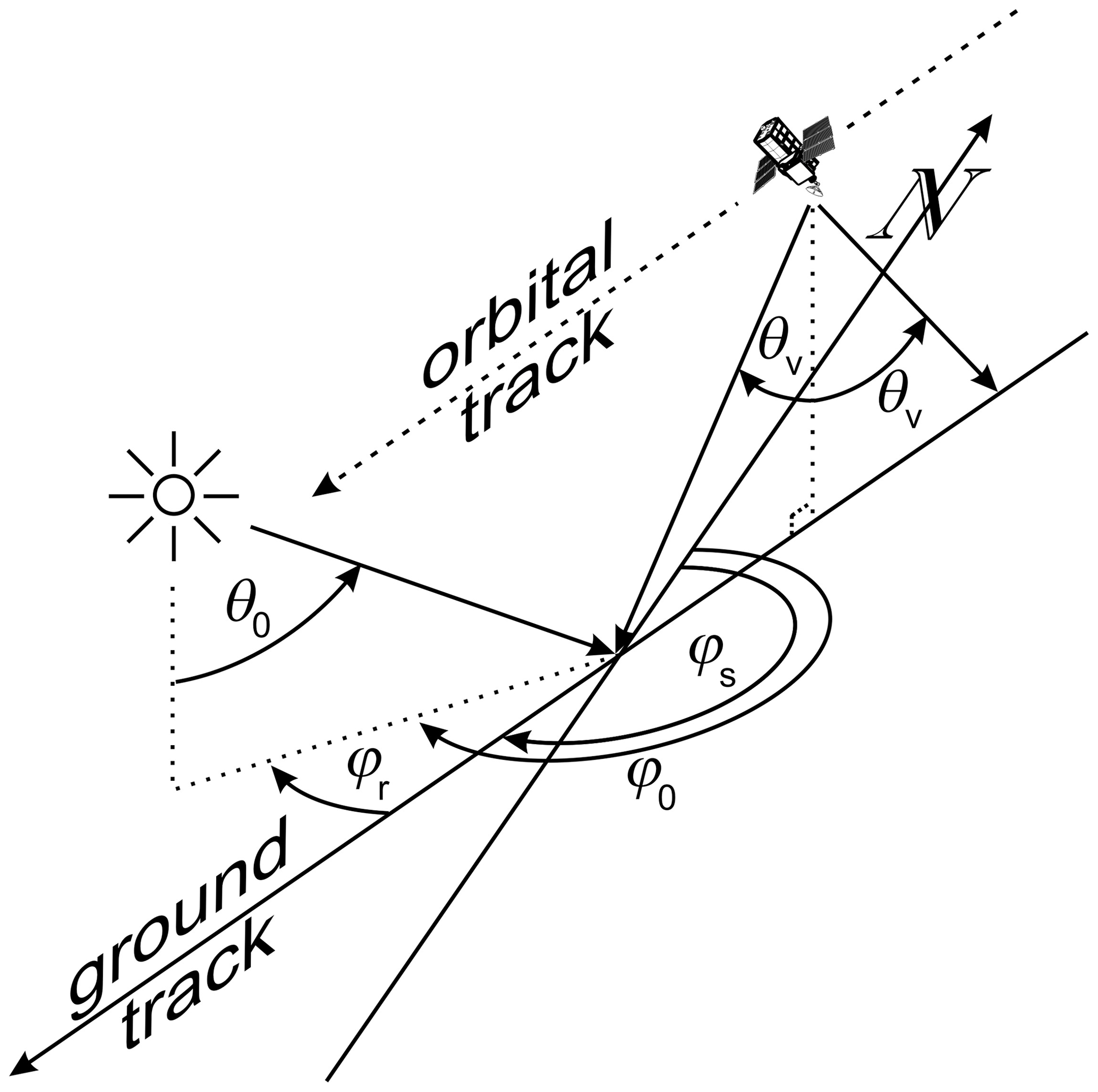
Figure 1 Schematic showing solar zenith angle θ₀, solar azimuth angle relative to north φ₀, satellite-tracking vectors relative to north φ_s, solar azimuth angle relative to satellite tracking direction φ_r, and the BBR's two off-nadir zenith angles θ_v.

Of those L2-plane pixels whose MSI radiances best resemble those at $(i,j\ne \mathrm{0})$, the one lying physically closest to $(i,j\ne \mathrm{0})$ becomes the donor, and its profiles of geophysical information get replicated at $(i,j\ne \mathrm{0})$. This procedure is performed for all $(i,j\ne \mathrm{0})$ across the MSI's swath; pixels at (i,0) donate to themselves. The result is construction of a 3D atmosphere–surface domain made up of profiles from the L2 plane. Correspondingly, MSI imagery are reconstructed, too. Figure 2 shows a schematic of the radiance-matching procedure. Hereinafter, values at (i,j) that are based on the SCA are indexed as $\left(m^{*}\right(i,j),\mathrm{0})$, which ties them back to the $m^{*}(i,j)$th column/pixel along the L2 plane.

Figure 2 (a) A swath of passive imagery and the location of an off-nadir pixel at (i,j) whose radiances match best with those along nadir at $(m^{*},\mathrm{0})$. (b) A schematic illustrating the attribution of the (recipient) column associated with the pixel at (i,j) to the (donor) column of information inferred from EarthCARE's active–passive measurements at $(m^{*},\mathrm{0})$.

2.2 Assessment domains and their buffer zones

The 3D RT models used for EarthCARE employ cyclic horizontal boundary conditions. Real cloudy domains and those produced by the SCA are, however, non-cyclical, and so when 3D RT models operate on them, adverse effects near the perimeter of D are affected by photon paths crossing discontinuous optical properties. One way to deal with this is to add atmosphere and surface to all edges of D so as to not eliminate but rather displace away from D any adverse effects set up by the assumed cyclic boundary conditions. Hereinafter, the domain resulting from the combination of D and its buffer zones is denoted as D⁺.

Figure 3 Schematic showing the radiative closure assessment domain D(i) (black) and the radiation computation domain D⁺(i), the union of D(i), and the buffer zone (shaded). See the text for definitions of indices.

Buffer zones also accommodate the fact that the BBR's oblique radiances associated with D consist partly of photons that were scattered by the atmosphere and surface outside of D. Barker et al. (2015) described an adjustment to 3D RT Monte Carlo models that approximates fractional contributions to a BBR radiance from photons whose last scattering event, by any particular scattering species, took place in D. Their algorithm, however, is too time-consuming for EarthCARE's official data-processing system. Nevertheless, the buffer zone should adequately capture contributions to BBR radiances that come from beyond D.

Setting the along- and across-track dimensions of buffer zones is described in detail in Appendix B. Figure 3 shows D, its associated D⁺, and the indices that locate them on the JSG. The number of pixels in the along-track direction that are out in front $n_{\mathrm{buffer}}^{\searrow }$ and trailing $n_{\mathrm{buffer}}^{\swarrow }D$ can vary and depend on the minimum along-track buffer length $d_{\parallel }^{min}$, assumed to be ∼5 km, BBR viewing zenith angle θ_v, and nearby cloud-top altitudes $h\left(m^{*}\right(i,j),\mathrm{0})$ as defined by the radiance-matching algorithm. Figure 4 is a schematic of this process, which is detailed in Appendix B.

Figure 4 Schematic showing the procedure for finding along-track buffer zone size – in this case $n_{\mathrm{buffer}}^{\swarrow }$. (a) $h_D^{max}$ is maximum cloud-top altitude in assessment domain D, and $d_{\parallel }^{min}$ is the smallest size buffer zone allowed. (b) As the algorithm searches out in front of D, a cloud is encountered, part of which lies between D and the satellite, and so the buffer zone increases. (c) Continuing the search, still a higher cloud is encountered between D and the satellite, thus increasing the buffer zone further. (d) There is still more cloud between D and the satellite so the buffer zone increases again, this time to its final value of $n_{\mathrm{buffer}}^{\swarrow }$, despite the possibility of cloud tops further out being higher yet still. See text and Appendix B for details.

Note that $n_{\mathrm{buffer}}^{\swarrow }$ and $n_{\mathrm{buffer}}^{\searrow }$ are independent of θ₀. This is because for EarthCARE's orbit, over 80 % of observations with ${\mathit{\theta }}_{\mathrm{0}}<\mathrm{90}{}^{\circ }$ have $\mathrm{30}{}^{\circ }<{\mathit{\phi }}_{\mathrm{r}}<\mathrm{150}{}^{\circ }$, implying that, for most cases, projection of a direct beam (and hence cloud shadows) into the along-track walls of D will be small. Exceptions are for very large θ₀ with ${\mathit{\phi }}_{\mathrm{r}}<\mathrm{30}{}^{\circ }$ or ${\mathit{\phi }}_{\mathrm{r}}>\mathrm{150}{}^{\circ }$, but these cases are usually avoided because the RT models rely on the plane-parallel approximation.

Determination of the size of cross-track buffer zones m_buffer depends on $h\left(m^{*}\right(i,j),\mathrm{0})$ adjacent to the sunlit side of D and minimum size for the across-track buffer zone $d_{\perp }^{min}$. If a cloud to the side of D casts a shadow that falls onto the region formed by D and its along-track buffer zones, then the cross-track buffer zone extends to include the cloud doing the shadowing. Unlike the along-track, m_buffer gets applied to both sides of D. Figure 5 summarizes definition of m_buffer.

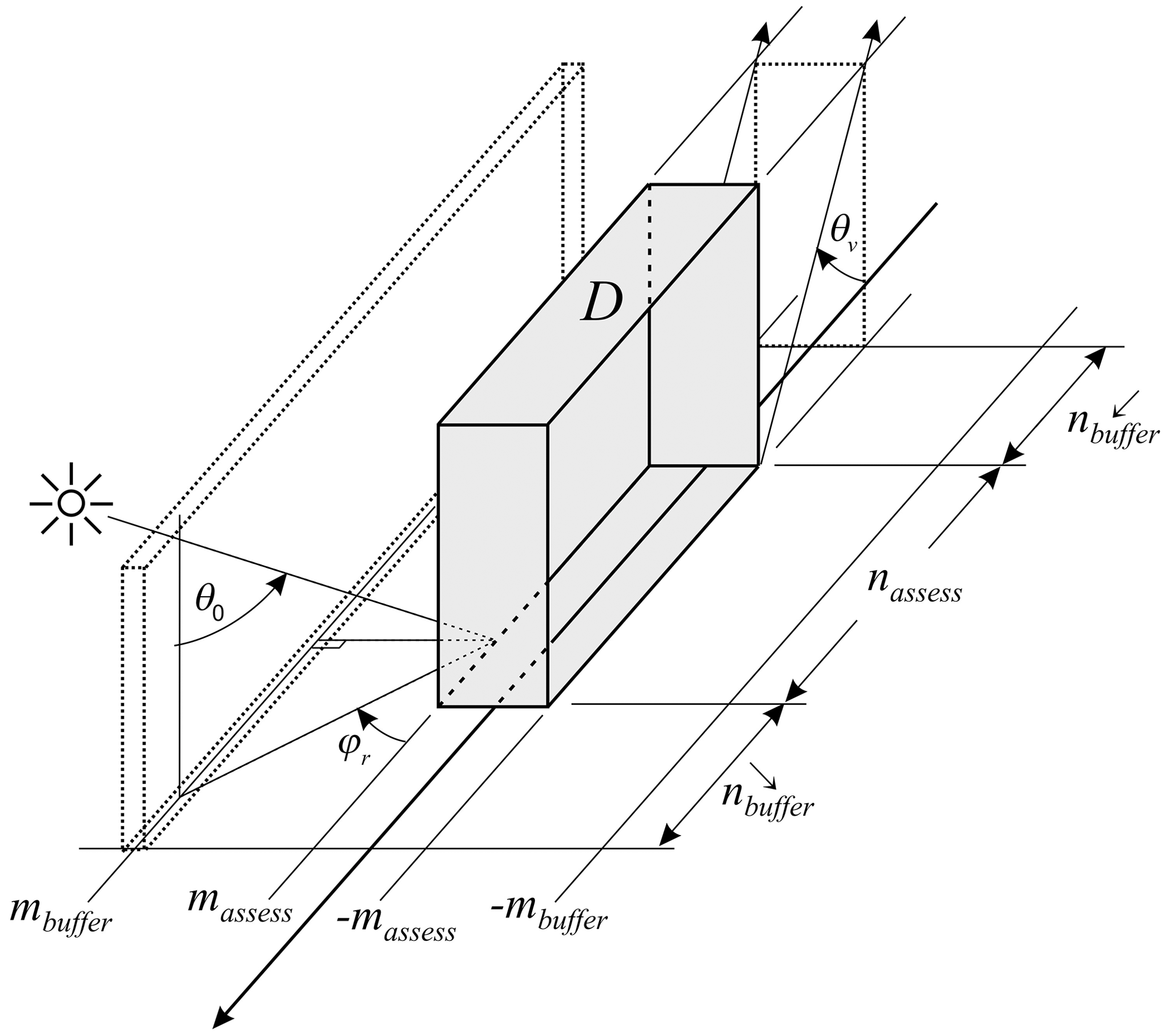
Figure 5 Schematic showing the procedure for finding the size of the cross-track buffer zone size m_buffer. See text and Appendix B for details.

2.3 Screening radiative closure assessment domains

Due to computational limitations and time constraints on product production, it is anticipated that only a small number of D per frame will participate in the 3D RT radiative closure exercise (i.e., processor ACMB-DF). Hence, domains D that emerge from the SCA must be screened and ranked to ensure that an adequate range of cases, from simple to complex, is assessed in order to (i) provide well-rounded pictures of algorithmic performances, (ii) gauge whether mission objectives are being met, and (iii) provide guidance to data users who wish to focus on select conditions. At the same time, screening and ranking should be flexible enough to be changed during the mission. For instance, simple scenarios are likely to be of particular interest during the commissioning phase (e.g., mono-phase, single-layer, overcast clouds).

The screening process eliminates domains D that are likely to yield uninformative assessments. It has three stages as described in the following subsections. Each frame has two sets of surviving assessment domains: D_1D contains domains that 1D RT results are averaged over and D_3D contains domains that 3D RT models get applied to. Domains in D_1D and D_3D consist, respectively, of radiative assessment domains D and radiative computation domains D⁺ (see Fig. 3).

2.3.1 Screening stage 1: failed retrievals and corrupt data

If there are corrupt data or failed retrievals for any column in either D or D⁺, the domain will not be forwarded to subsequent processes. This is because they simply cannot be used by 3D RT models. Examples of failed retrievals include algorithms that did not converge to a solution or converged to values that are out of bounds. Corrupt data, on the other hand, include failure at the L1 level and data corrupted during transmission.

2.3.2 Screening stage 2: geophysical conditions

(a) Solar zenith angle

Generally speaking, solar RT becomes increasingly complicated as solar zenith angle θ₀ increases. This is because (i) radiances and fluxes for EarthCARE-sized domains will depend increasingly on conditions outside D and D⁺ and (ii) Earth's sphericity becomes increasingly important and EarthCARE's RT codes are plane-parallel models. Not only do large θ₀ values impact the SCA directly, they stress retrieval algorithms that use MSI data. Hence, when the Sun is up, D or D⁺ must have

$$\begin{array}{}\text{(1)}& max\left\{{\mathit{\theta }}_{\mathrm{0}}(i,j)\right\}<{\mathit{\theta }}_{\mathrm{0}}^{*}\forall (i,j)\in D\text{or}{D}^{+},\end{array}$$

where ${\mathit{\theta }}_{\mathrm{0}}^{*}$ is the maximum allowed value of θ₀, in order for solar radiances to be considered by the SCA. Initially, ${\mathit{\theta }}_{\mathrm{0}}^{*}=\mathrm{75}{}^{\circ }$. When the Sun is down, however, data from solar channels are simply not used; as shown by Barker et al. (2011), this diminishes the SCA's performance.

(b) Single surface type

To focus closure assessments on retrieved cloud and aerosol properties and reduce potential complications due to boundary conditions that are outside the purview of EarthCARE's retrievals, D and D⁺ must have at least 90 % of their area occupied by a single broad class of surface type. These types are water (oceans and lakes), land, and ice.

(c) Homogeneous land surfaces

Each JSG pixel has a land-type designation obtained from the International Geosphere–Biosphere Programme (USGS, 2018). Let f_ℓ be the fraction of JSG pixels in either D or D⁺ that corresponds to the ℓth surface type. For reasons listed above, if D and D⁺ are a land domain, then for them to be included in D_1D and D_3D, they must have

$$\begin{array}{}\text{(2)}& max\left\{f_{\mathrm{\ell }}\right\}>f^{*},\end{array}$$

where f^* is set initially to 0.9.

(d) Surface elevation

Uncertainties in spectral bidirectional reflectance and emittance functions as well as albedos and emissivities are complicated by variations in surface elevation. In an attempt to limit uncertainties associated with the setting of these lower boundary conditions in the RT models, only very flat assessment domains are allowed. Hence, if σ_srf is standard deviation of surface elevation for D or D⁺, then for them to be included in D_1D and D_3D, they  must have

$$\begin{array}{}\text{(3)}& {\mathit{\sigma }}_{\mathrm{srf}}<{\mathit{\sigma }}_{\mathrm{sfc}}^{*},\end{array}$$

where ${\mathit{\sigma }}_{\mathrm{sfc}}^{*}$ is set initially to 0.1 km.

2.3.3 Screening stage 3: quality of radiance matching

Where SCA reconstructed MSI radiances are poor, it is reasonable to assume that corresponding constructed 3D domains are too. Thus, the final screening stage addresses the quality of reconstructed MSI imagery, but it also provides bias-correction estimates for modelled TOA quantities.

For an assessment domain D of n_assess JSG pixels along-track and $j\in \left[-m_{\mathrm{assess}},m_{\mathrm{assess}}\right]$ across-track, the nth moment of r_k over D, excluding the L2 line along j=0, is

$$\begin{array}{}\text{(4)}& \begin{array}{rl}& 〈r_k^n〉\\ & ={\displaystyle \frac{\mathrm{1}}{\mathrm{2}{m}_{\mathrm{assess}}{n}_{\mathrm{assess}}}}\sum _{i=i_{\mathrm{1}}}^{i_{\mathrm{1}}+n_{\mathrm{assess}}-\mathrm{1}}\sum _{j\in \left[-m_{\mathrm{assess}},-\mathrm{1}\right]\cup \left[\mathrm{1},m_{\mathrm{assess}}\right]}{r}_k^n(i,j),\end{array}\end{array}$$

where i₁ is the along-track JSG index at the edge of D. Corresponding reconstructed values are

$$\begin{array}{}\text{(5)}& \begin{array}{rl}& 〈{\widehat{r}}_k^n〉\\ & ={\displaystyle \frac{\mathrm{1}}{\mathrm{2}{m}_{\mathrm{assess}}{n}_{\mathrm{assess}}}}\sum _{i=i_{\mathrm{1}}}^{i_{\mathrm{1}}+n_{\mathrm{assess}}-\mathrm{1}}\sum _{j\in \left[-m_{\mathrm{assess}},-\mathrm{1}\right]\cup \left[\mathrm{1},m_{\mathrm{assess}}\right]}{r}_k^n\left(m^{*}\right(i,j),\mathrm{0}).\end{array}\end{array}$$

Therefore, errors stemming from the radiance-matching algorithm, for the kth MSI channel, are

$$\begin{array}{}\text{(6)}& \mathrm{\Delta }〈{\widehat{r}}_k^n〉=〈{\widehat{r}}_k^n〉-〈r_k^n〉.\end{array}$$

Let 〈F_SW〉 and 〈F_LW〉 be TOA shortwave (SW) and longwave (LW) fluxes, averaged over D, as estimated by angular direction models in the BMA-FLX processor (Velázquez-Blázquez et al., 2023). Since MSI radiances r₁ (0.67 µm) and r₆ (10.80 µm) often correlate well with 〈F_SW〉 and 〈F_LW〉 (Barker et al., 2014), TOA flux bias errors due to the radiance-matching algorithm can be approximated as

$$\begin{array}{}\text{(7)}& \begin{array}{rl}& \mathrm{\Delta }〈{\widehat{F}}_{\mathrm{SW}}〉\approx 〈F_{\mathrm{SW}}〉{\displaystyle \frac{〈r_{\mathrm{1}}〉-〈{\widehat{r}}_{\mathrm{1}}〉}{〈{\widehat{r}}_{\mathrm{1}}〉}}\text{and}\\ & \mathrm{\Delta }〈{\widehat{F}}_{\mathrm{LW}}〉\approx 〈F_{\mathrm{LW}}〉{\displaystyle \frac{〈r_{\mathrm{6}}〉-〈{\widehat{r}}_{\mathrm{6}}〉}{〈{\widehat{r}}_{\mathrm{6}}〉}}.\end{array}\end{array}$$

If these values satisfy

$$\begin{array}{}\text{(8)}& \left|\mathrm{\Delta }〈{\widehat{F}}_{\mathrm{SW}}〉\right|>\mathrm{\Delta }{F}_{\mathrm{SW}}^{*}{\mathit{\mu }}_{\mathrm{0}}\text{and}\left|\mathrm{\Delta }〈{\widehat{F}}_{\mathrm{LW}}〉\right|>\mathrm{\Delta }{F}_{\mathrm{LW}}^{*},\end{array}$$

where $\mathrm{\Delta }{F}_{\mathrm{SW}}^{*}$ and $\mathrm{\Delta }{F}_{\mathrm{LW}}^{*}$ are tolerable broadband TOA flux errors arising from the radiance-matching algorithm, D is not included in either D_1D or D_3D. Both $\mathrm{\Delta }〈{\widehat{F}}_{\mathrm{SW}}〉$ and $\mathrm{\Delta }〈{\widehat{F}}_{\mathrm{LW}}〉$ get passed to ACMB-DF and used to bias-correct estimated TOA fluxes made by both 1D and 3D RT models. This completes the screening processes leaving D_1D and D_3D with m_1D and m_3D assessment domains, respectively.

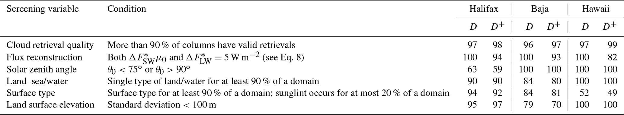
Table 1 provides a glimpse into success rates of D and D⁺, in all three frames, for the screenings just described using conditions as summarized in the table. Of course, overall success rate for ${\mathit{\theta }}_{\mathrm{0}}<\mathrm{75}{}^{\circ }$ will be much smaller than most reported here owing to these being descending frames. Note also the tendency for success rates for D⁺ to be less than those for D. This is because the areal extents of D⁺ are always larger than that for D.

Table 1 Success rates of D and D⁺ for the three frames that meet the conditions as listed.

2.4 Ranking radiative assessment domains

As noted above, the EarthCARE mission will provide near-real-time products with limited computational resources. The portion of the processing chain constrained most by this involves 3D SW RT models. For them to achieve adequate signal-to-noise ratios, just a small fraction of the thousands of potential domains D⁺ per frame can be assessed. Thus, to enhance efficacy of the radiative assessment process, an algorithm was developed that ranks D⁺ in D_3D. At any time, ranking can be overruled manually, such as when testing during the commissioning phase. The ranking algorithm that was decided upon samples cloud scenarios in proportion to relative frequencies of occurrence.

For the initial version of the algorithm, 1 km resolution MODIS-retrieved values (MYD06_L2) of cloud optical depth τ_cld and cloud-top pressure p_cld, inferred from measurements made during 2020, were grouped into 5×21 km arrays to match EarthCARE's planned 5×21 km domains D, and for each array, mean values 〈τ_cld〉 and 〈p_cld〉 were computed along with total cloud fraction A_c (Platnick et al., 2015). They were then assigned to bins defined by 10^∘ ranges of latitude and longitude, as well as ranges for 〈τ_cld〉, 〈p_cld〉, A_c, and time of observation of

$$\begin{array}{}\text{(9)}& \begin{array}{ll}〈{\mathit{\tau }}_{\mathrm{cld}}〉& :(\mathrm{0},\mathrm{4}];(\mathrm{4},\mathrm{23}];(\mathrm{23},\mathrm{150}]\\ 〈p_{\mathrm{cld}}〉& :(\mathrm{0},\mathrm{440}];(\mathrm{440},\mathrm{680}];(\mathrm{680},\mathrm{\infty })\\ A_{\mathrm{c}}& :(\mathrm{0},\mathrm{0.25}];(\mathrm{0.25},\mathrm{0.75}];(\mathrm{0.75},\mathrm{0.99}];(\mathrm{0.99},\mathrm{1}]\\ \text{time}& :\text{DJF};\text{MAM};\text{JJA};\text{SON}.\end{array}\end{array}$$

Since only cloud-bearing domains need be ranked, the number of applicable bins is 23 328, of which the nth has N_n domains. When ${\mathit{\theta }}_{\mathrm{0}}\ge \mathrm{90}{}^{\circ }$, 〈τ_cld〉 is not retrieved, so the same ranking procedure uses the remaining three variables only. Radiative closure assessments for SW fluxes are not done when $\mathrm{75}{}^{\circ }<{\mathit{\theta }}_{\mathrm{0}}<\mathrm{90}{}^{\circ }$ on account of too many overwhelming uncertainties with retrievals and plane-parallel RT modelling. Thus, domains in this range are not ranked.

For EarthCARE frames with 5000 1 km L2 columns in the L2 plane, there is the potential for $\mathrm{5000}-\mathrm{21}+\mathrm{1}=\mathrm{4980}$ (over-sampled) assessment domains, each of which falls into one of the MODIS bins. Now, using only domains with A_c>0.01, form the frame-specific cumulative frequency such that the ith domain has a value

$$\begin{array}{}\text{(10)}& N\left(i\right)={\displaystyle \frac{\mathrm{1}}{N\left(\mathrm{4980}\right)}}\sum _{j=\mathrm{1}}^i{N}_n\left(j\right);i=\mathrm{1},\mathrm{\dots },N_{\mathrm{cld}}\le \mathrm{4980}.\end{array}$$

Then, generate a uniform pseudo-random number $R\in (\mathrm{0},\mathrm{1}]$ and find the closest N(i); this identifies the top-ranked D⁺. This is repeated, without replacement, until (possibly all) the domains are ranked. The resulting lists are passed on to ACM-RT.

3 Results

The SCA's sub-algorithms are discussed in series in this section. The only part not evaluated here is the ranking algorithm (see Sect. 2.4). Its performance is demonstrated in Cole et al. (2022; in this issue) where radiative transfer models act on the highest ranked assessment domains.

3.1 Reconstruction of passive radiances

Radiance matching is the essence of the SCA, and a sampling of results is provided here. More details are in Barker et al. (2011, 2012, 2014) and Sun et al. (2016). All results presented here, and when ${\mathit{\theta }}_{\mathrm{0}}<\mathrm{90}{}^{\circ }$, come from using MSI channels: 1 (0.67 µm), 4 (2.21 µm), 5 (8.80 µm), and 7 (12.00 µm); i.e., K_s=4 in Eq. (A1). Obviously, when ${\mathit{\theta }}_{\mathrm{0}}\ge \mathrm{75}{}^{\circ }$ the SW channels are not used. The largest impediment facing this algorithm is when conditions off the ground track (GT) differ much from the relatively few samples along the GT (Barker et al., 2011). Figure 6 shows a full-width segment of the Hawaii frame that contains both catastrophic failure due to inadequate conditions along the GT and excellent performance for the opposite reason. Approximately 50–100 km east of the GT, between 9.5 and 13^∘ N, radiances, especially channel 1's, that are associated with much cloud are severely short-changed on account of a long stretch of near-cloudless conditions at nadir. To partially remedy this, the algorithm would have to be permitted to search the GT much further than 200 km, as in this example, but in so doing it would run the risk of identifying donor columns associated with increasingly different meteorological conditions. On the other hand, between 5 and 8^∘ N performance is extremely good across the entire 150 km wide frame.

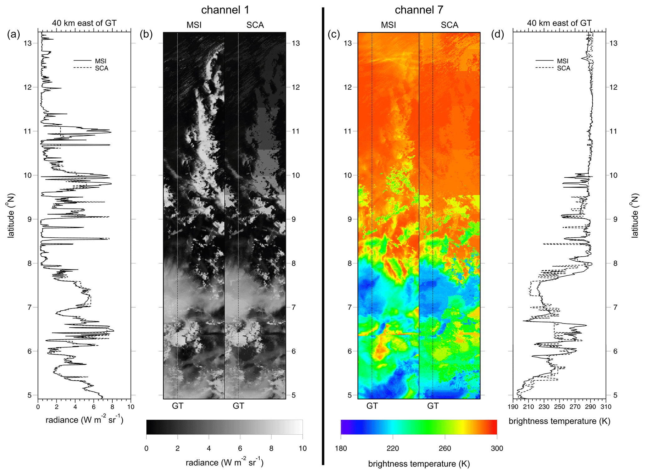
Figure 6 (a, b) MSI and corresponding SCA channel 1 radiances for a segment of the Hawaii frame measuring 150 km wide and 900 km long. (c, d) Corresponding brightness temperatures from channel 7 radiances. Dashed lines marked GT indicate the ground track at nadir, which coincides with the L2 plane. Line graphs show MSI and SCA values along the centres of the domains, which are 40 km east of GT.

Figure 7 shows mean bias errors (MBEs) and root mean square errors (RMSEs) for reconstructed MSI channels 1 and 7 as functions of distance, east and west, of GT for the full lengths of the three test frames (see Qu et al., 2022). By definition, MBE and RMSE along GT are zero. For channel 1's reconstructions, MBEs out to ±20 km are generally smaller than 0.05 W m⁻² sr⁻¹, with smaller errors for cloudless pixels. The negative biases for Baja and Hawaii frames out past ∼5 km from GT stem from clouds along the GT being slightly darker than those elsewhere over the frames (see Fig. 6). Likewise, MBEs for channel 7 are generally smaller than 0.5 K. Over the 5 km wide assessment domains centred on GT, MBEs for both channels are almost negligible relative to the frame-wide average values that are listed along the base of each plot.

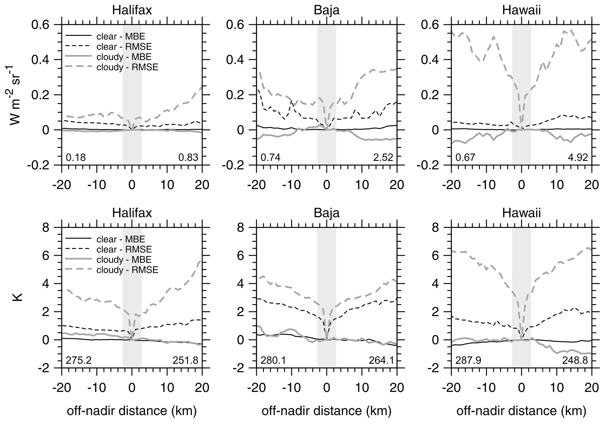
Figure 7 Full-frame mean bias errors (MBEs) and root mean square errors (RMSEs) for SCA reconstructed radiances as functions of distance (negative values are W) from the ground track (GT in Fig. 6). Upper and lower rows are for MSI channel 1 radiances and channel 7 brightness temperatures. Full-frame mean values are listed on the base of each plot: clear sky on the left and cloudy sky on the right. Grey bands indicate EarthCARE's default assessment domains.

Unlike MBEs, however, RMSE values jump immediately off the GT. In general, they continue to increase with distance from GT, but it is difficult to say at what distance they become unusable. It is important to note that RMSE values plotted here get reduced by at least a factor of 10 for averages over assessment domains.

3.2 Definition of assessment domain buffer zones

The planned initial default values for both $d_{\parallel }^{min}$ and $d_{\perp }^{min}$ is 5 km. Thus, for D measuring 5×21 km, 3D RT will be applied to domains D⁺ that measure at least ∼15 km across-track by ∼31 km along-track. Figure 8 shows sizes of D⁺ along the Hawaii frame. The most notable feature is that along-track lengths vary much more than across-track lengths. This is driven by the fixed along-track off-nadir views of the BBR; whenever cloud occurs, especially high cloud, values of $n_{\mathrm{buffer}}^{\searrow }$ and $n_{\mathrm{buffer}}^{\swarrow }$ exceed 0. Lengths of D⁺ maximize between about 3 and 6^∘ N, where mean cloud-top altitudes h reach ∼17 km; this is despite cloud fractions for D⁺ being substantially less than 1.

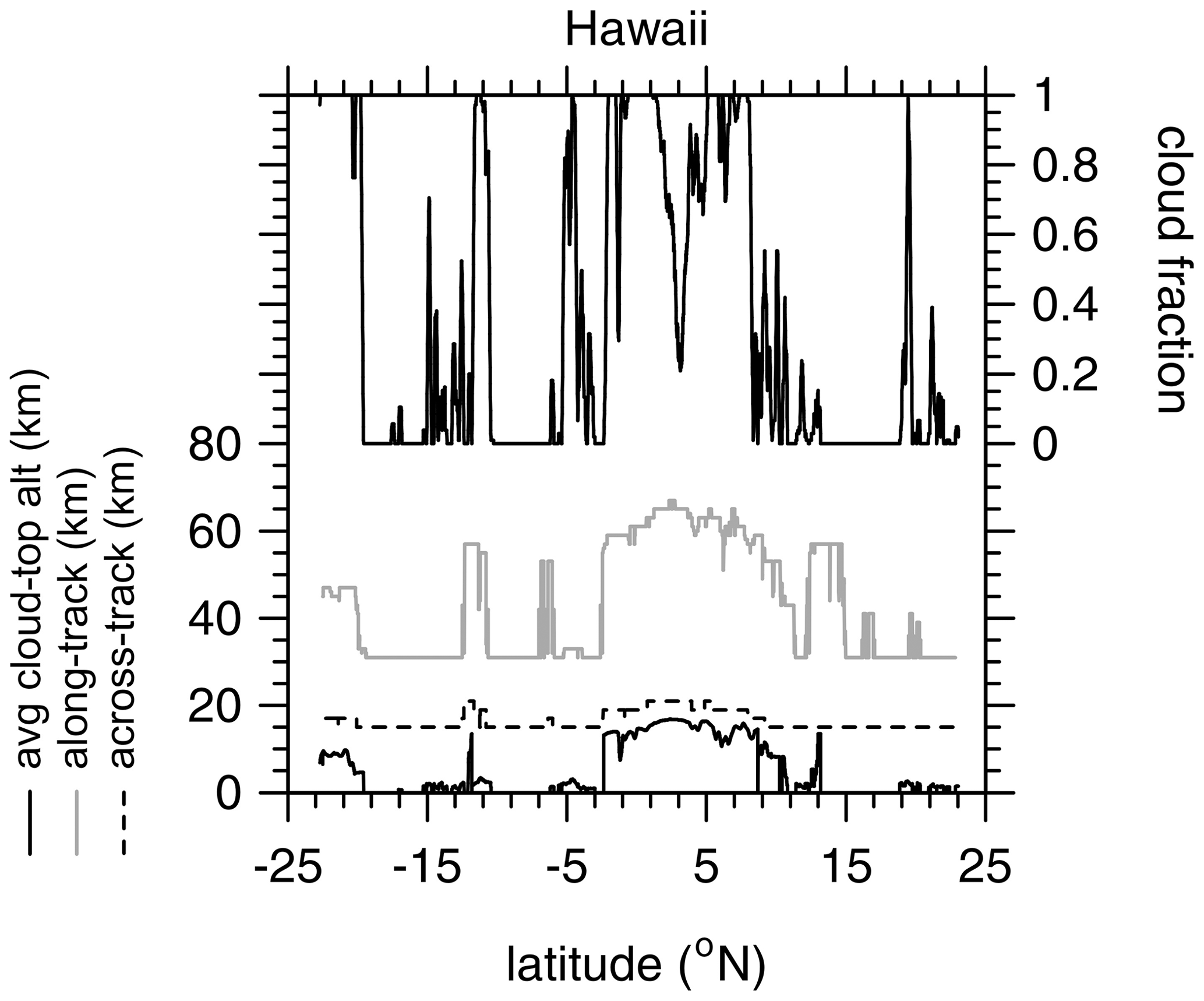
Figure 8 Along-track and across-track length of assessment domain plus buffer zones as functions of latitude for the Hawaii frame. All assessment domains are 5 km across-track by 21 km along-track. The minimum size for all buffer zones is 5 km. Also shown are corresponding values of mean cloud-top altitude and cloud fraction for 5×21 km assessment domains.

While across-track buffer sizes m_buffer depend on h, too, they also depend on φ_r and θ₀. Near latitude 10^∘ N, while ${\mathit{\phi }}_{\mathrm{r}}\approx \mathrm{107}{}^{\circ }$ (Sun is shining almost perpendicular to GT), ${\mathit{\theta }}_{\mathrm{0}}\approx \mathrm{30}{}^{\circ }$ and lengths of cloud shadows cast perpendicular to GT are small. As such, there is little need to expand the domain across-track, and so m_buffer=0 and cross-track size of D⁺ equal the default 15 km. Near latitude 21^∘ S, however, where mean h values are the same as near 10^∘ N, clouds are more overcast, but equally important, ${\mathit{\phi }}_{\mathrm{r}}\approx \mathrm{130}{}^{\circ }$, which is still not far off shining perpendicular to GT, and ${\mathit{\theta }}_{\mathrm{0}}\approx \mathrm{50}{}^{\circ }$. Together these conspire to cast cloud shadows well beyond D, resulting in domains D⁺ that are slightly larger than the default.

3.3 Estimation of SCA-related bias errors for TOA broadband fluxes

In a manner similar to cloud radiative effects, estimation of errors for TOA broadband radiative fluxes that arise from the SCA process provide a simple, integrated indication of SCA performance. Figure 9 shows cumulative frequency distributions of $\mathrm{\Delta }〈{\widehat{F}}_{\mathrm{SW}}〉$ and $\mathrm{\Delta }〈{\widehat{F}}_{\mathrm{LW}}〉$ (see Eq. 7) for the Hawaii frame. Errors for this frame are the largest of the three. As is often the case, errors tend to be largest for SW fluxes and increase slightly as assessment domain A_c increases. The latter point basically indicates that the SCA does extremely well in clear-sky conditions, even for the Baja frame that was mostly over variable land.

It is encouraging to see that median errors for both bands are negligible for all conditions. Moreover, as Fig. 9 shows, with ∼90 % of errors being within ±3 W m⁻², and slightly better for the other frames, errors imparted on TOA flux estimates by the SCA will not hinder assessment of EarthCARE's objective of retrieving cloud–aerosol properties well enough as to be able to model, on average, TOA fluxes to within ±10 W m⁻².

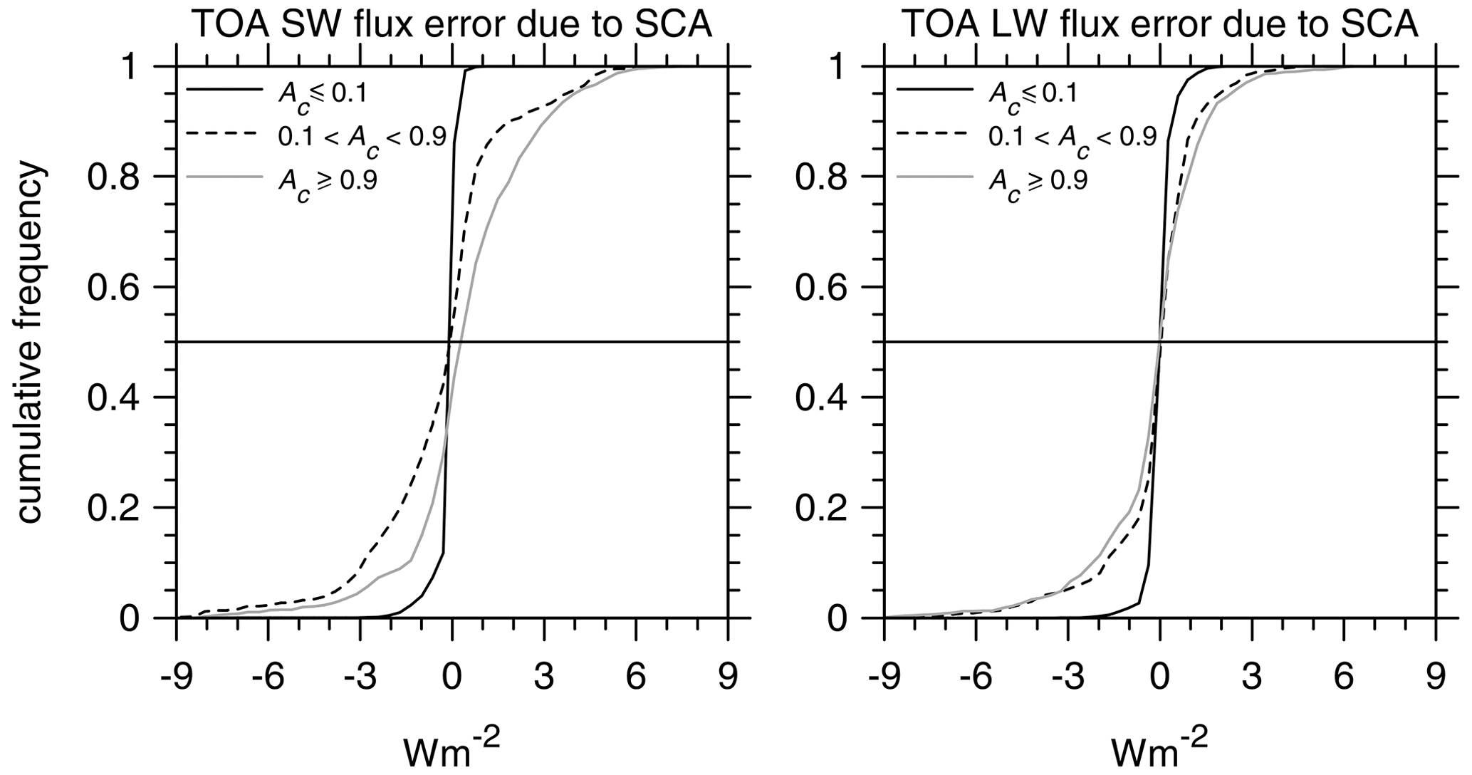
Figure 9 Cumulative frequency distributions of estimated errors in broadband TOA upwelling SW and LW fluxes stemming from the SCA for all 5×21 km assessment domains in the Hawaii frame. Distributions are partitioned for three ranges of assessment domain total cloud fraction A_c.

4 Summary and discussion

The EarthCARE satellite mission has set itself a very high bar with its plan to infer cloud and aerosol properties, from its observations, well enough that when used to initialize radiative transfer (RT) models, their estimates of TOA fluxes will differ from observed values by, typically, less than ±10 W m⁻². To realize and gauge the success of this radiative closure assessment it will be necessary to employ, operationally, 3D atmospheric RT models. This by itself will set EarthCARE apart from its predecessors, which have relied entirely on 1D RT models. The immediate issue facing this plan is that L2 retrievals at nadir are just ∼1 km wide, and at this scale net fluxes of lateral flowing radiation, not accounted for by 1D RT models, can be substantial (e.g., Marshak et al., 1998). To justifiably use 3D RT models, however, the atmosphere–surface system has to be defined on both sides of the narrow L2 plane. The point of this paper was to demonstrate EarthCARE's method of expanding its L2 retrievals perpendicular to the L2 plane. At the core of this 3D scene construction algorithm (SCA) is a radiance-matching (RM) scheme that uses EarthCARE's MSI passive imagery (cf. Barker et al., 2011, 2012, 2014). There are, however, other aspects of this process that have been documented here for the first time.

Synthetic radiances measured virtually by EarthCARE's MSI for three test frames, which were produced for end-to-end simulation of EarthCARE's measurement-processing chain (see Qu et al., 2022), were used here to demonstrate the performance of the SCA. Reconstruction of measured MSI radiances forms the foundation of the SCA. Basically, off-nadir pixels are paired with a nadir pixel whose spectral radiances best match theirs. The 3D domains to be used by the 3D RT models are constructed by taking columns of geophysical information associated with matching nadir pixels and inserting them at the off-nadir pixels.

Comparing reconstructed radiances to their observed counterparts provides a straightforward indication of the success of the SCA. If observed radiances are reconstructed poorly, one has to also assume that correspondingly constructed 3D surface–atmosphere domains are unfit for both 3D RT models and radiative closure assessment. SCA errors flare up when conditions needed at off-nadir locations are lacking from the nearby the L2 plane. Typical performances of the SCA are shown in Sect. 3.1 and, as expected, generally erode the further recipient pixels are from their donors. This is not much of an issue for radiative assessment domains themselves, for they extend just 2 km from the L2 plane. Their buffer zones, however, which are described in Sect. 2.2, can be as much as 10 km from the L2 plane (see Fig. 3). The reason why assessment domains are so small is because EarthCARE's radiative closure assessment seeks to verify the narrow L2 retrievals and not the SCA; the SCA should help achieve this as invisibly as possible.

Once defined, assessment domains and their buffer zones get screened (see Sect. 2.3) in an attempt to identify those most likely to realize useful closure assessments. Furthermore, the intersection of EarthCARE's data-processing limitations with the computational demand of the 3D solar RT model (Cole et al., 2022) forces the need to rank assessment domains to ensure that the few that get assessed per frame lead to good samplings, over the mission's life, of conditions that occur over the globe and the year. This process is described in Sect. 2.4.

The simple method of estimating TOA flux bias errors that are likely to arise from the SCA (Barker et al., 2014) was assessed using test frame synthetic observations. Reassuringly, it is shown in Sect. 3.3 that most TOA flux errors due to the SCA's imperfect atmospheres, for assessment domains measuring 5×21 km, can be expected to be much smaller, and rarely larger, than EarthCARE's stated goal of ±10 W m⁻².

To conclude, it is tempting to view the SCA as a very cost-effective (i.e., almost free) scanning active sensor system (cf. Illingworth et al., 2018). But one almost always gets what one pays for, and the SCA is, when pushed, no exception. Its performance, especially well removed from the L2 plane, cannot be expected to rival that of an authentic scanning active sensor system (Barker et al., 2021); to use it as a full-up replacement would be cavalier. In its current role, however, as purveyor of approximate, ancillary information that both facilitates use of 3D RT models and strengthens verification of L2 retrievals, it appears as though its shortcomings will be tolerable and outweighed by its benefits.

Appendix A: Radiance-matching algorithm

Let r_k(i,j) be MSI radiance, for the kth MSI channel, at (i,j) on the joint standard grid (JSG) in which j=0 is along the L2 plane. Following Barker et al. (2011), when seeking to populate a column at $\left(i,j\ne \mathrm{0}\right)$ with a suitable proxy from $\left(i,j=\mathrm{0}\right)$, begin by computing, for K_s channels,

$$\begin{array}{}\text{(A1)}& \begin{array}{rl}& F(i,j;m)\\ & =\mathrm{\Lambda }(i,j;m)\sum _{k=\mathrm{1}}^{K_s}{a}_k{\left[{\displaystyle \frac{r_k(i,j)-r_k(m,\mathrm{0})}{max\left[r_k(i,j),r_k(m,\mathrm{0})\right]}}\right]}^{\mathrm{2}};\\ & m\in \left[i-M,i+M\right];j\notin \mathrm{0},\end{array}\end{array}$$

where (m,0) holds potential donor profiles for the recipient at $(i,j\ne \mathrm{0})$, a_k represents weights that could depend on channel but were assumed to equal 1, and M is number of pixels, forward and backward, along the L2 plane to be searched for a donor. The function $\mathrm{\Lambda }(i,j;m)$ is defined as

$$\begin{array}{}\text{(A2)}& \mathrm{\Lambda }(i,j;m)=\left\{\begin{array}{rl}-\mathrm{1};& \mathit{\chi }=\text{.false.}\\ \mathrm{1};& \mathit{\chi }=\text{.true.}\end{array}\right.\end{array}$$

By requiring

$$\begin{array}{}\text{(A3)}& \mathit{\chi }=\left\{\begin{array}{c}\text{surface at}(i,j)=\text{surface at}(m,\mathrm{0})\\ \text{.and.}\\ \left|{\mathit{\mu }}_{\mathrm{0}}(i,j)-{\mathit{\mu }}_{\mathrm{0}}(m,\mathrm{0})\right|<\mathrm{\Delta }{\mathit{\mu }}_{\mathrm{0}}\\ \text{.and.}\\ {\mathit{\mu }}_{\mathrm{0}}(i,j)\cdot {\mathit{\mu }}_{\mathrm{0}}(m,\mathrm{0})>\mathrm{0}\\ \text{.and.}\\ \left|{\mathit{\phi }}_{\mathrm{r}}(i,j)-{\mathit{\phi }}_{\mathrm{r}}(m,\mathrm{0})\right|<\mathrm{\Delta }{\mathit{\phi }}_{\mathrm{r}}\\ \text{.and.}\\ m\in \left[\mathrm{1},N_{\mathrm{JSG}}\right],\end{array}\right.\end{array}$$

it controls whether or not a pixel at (m,0) is to be considered as a potential donor (see Sect. 2.3). The upper condition means that surface types (land, sea, and snow/ice) must be the same at (i,j) and (m,0). The next two conditions mean that at (i,j) and (m,0) cosine of solar zenith angles μ₀ must differ by less than Δμ₀=0.005, and the Sun must be up or down at both locations. Next, the difference between solar azimuth angles relative to the satellite's tracking direction φ_r must be less than $\mathrm{\Delta }{\mathit{\phi }}_{\mathrm{r}}=\mathrm{5}{}^{\circ }$. The final condition simply means that the search cannot go past the ends of a frame. It almost goes without saying, but when the Sun is down at (m,0), SW radiances are simply not used in Eq. (A1).

For the $\mathrm{1}\le M^{\prime }\le \mathrm{2}M+\mathrm{1}$ values of $F(i,j;m)\ge \mathrm{0}$ that get computed, define Euclidean distances between the centres of (i,j) and (m,0) as

$$\begin{array}{}\text{(A4)}& L(i,j;m)=\mathrm{\Delta }L{\left[(i-m{)}^{\mathrm{2}}+j^{\mathrm{2}}\right]}^{\mathrm{1}/\mathrm{2}},\end{array}$$

where ΔL is horizontal resolution, which for EarthCARE is ∼1 km, and sort $F(i,j;m)$ from smallest to largest (i.e., best to worst radiance match), with $L(i,j;m)$ going along passively. Denote the reordered sequences as ${\left\{\widehat{F}(i,j;m)\right\}}_{m=\mathrm{1}}^{M^{\prime }}$ and ${\left\{\widehat{L}(i,j;m)\right\}}_{m=\mathrm{1}}^{M^{\prime }}$. Finally, the donor for location $(i,j\ne \mathrm{0})$ is deemed to reside at

$$\begin{array}{}\text{(A5)}& m^{*}(i,j)=\underset{m\in \left[\mathrm{1},M^{\prime }\cdot f\right]}{\text{argmin}}\left\{\widehat{L}(i,j;m)\right\},\end{array}$$

which reads as follows: find m that corresponds to the smallest distance between the recipient at (i,j) and those pixels that constitute the smallest 100f % of $\widehat{F}(i,j;m)$. The tuneable parameter f will be set initially to 0.05, but this could change (see Barker et al., 2011). The procedure outlined here is performed for all $(i,j\ne \mathrm{0})$ across the MSI's swath, with pixels at (i,0) donating to themselves.

Appendix B: Calculation of buffer zone sizes

B1 Along-track length

Let $h\left(i^{\ast }(i,j),\mathrm{0}\right)$ be cloud-top altitude at JSG cell (i,j) using the SCA's field. Using these values, define for each i in a frame the highest cloud top in across-track swaths of JSG pixels spanning the assessment domains as

$$\begin{array}{}\text{(B1)}& h_{\perp }^{max}\left(i\right)=max\left\{h\left(i^{\ast }(i,j),\mathrm{0}\right)\right\}:j\in \left[-m_{\mathrm{assess}},m_{\mathrm{assess}}\right].\end{array}$$

The symbols ⊥ and ∥ indicate across- and along-tracks, respectively. Thus, the maximum cloud-top altitude in an assessment domain D(n) is

$$\begin{array}{}\text{(B2)}& h_D^{max}\left(n\right)=max\left\{h_{\perp }^{max}\left(i\right)\right\}:i\in \left[n,n+n_{\mathrm{assess}}-\mathrm{1}\right].\end{array}$$

Consider first the buffer zone out in front of D(n); applicable most to the BBR's backward view. The minimum number of JSG pixels that one needs be concerned about searching to see if clouds outside of D(n) obscure part of D(n) is

$$\begin{array}{}\text{(B3)}& n_{\mathrm{buffer}}=\text{nint}\left({\displaystyle \frac{max\left\{d_{\parallel }^{min},h_D^{max}\left(n\right)\tan {\mathit{\theta }}_{\mathrm{v}}\right\}}{〈\mathrm{\Delta }x〉}}\right),\end{array}$$

where $d_{\parallel }^{min}$ is the absolute minimum along-track buffer length, assumed for EarthCARE to be ∼5 km; θ_v is the BBR viewing zenith angle; and 〈Δx〉 is the mean length of JSG pixels in the along-track direction. For EarthCARE, 〈Δx〉≈1 km. If maximum cloud-top altitude across the entire useable part of the 5000 km frame is

$$\begin{array}{}\text{(B4)}& \begin{array}{rl}{h}_{\mathrm{F}}^{max}& =max\left\{h(i,j)\right\}:i\in \left[m_{\mathrm{1}}+\mathrm{1},N_{\mathrm{JSG}}-m_{\mathrm{2}}+\mathrm{1}\right],\\ & j\in \left[-m_{\mathrm{assess}},m_{\mathrm{assess}}\right],\end{array}\end{array}$$

then the absolute maximum number of JSG pixels one needs to search for outside of D(n) that might obscure part of D(n) is

$$\begin{array}{}\text{(B5)}& n_{\mathrm{buffer}}^{max}\approx \text{nint}\left({\displaystyle \frac{h_{\mathrm{F}}^{max}\tan {\mathit{\theta }}_{\mathrm{v}}}{〈\mathrm{\Delta }x〉}}\right).\end{array}$$

This can be reduced by knowing the location of the along-track JSG pixel that houses the highest cloud between the last pixel of D(n) and $n_{\mathrm{buffer}}^{max}$ pixels out in front of it. This is expressed as

$$\begin{array}{}\text{(B6)}& \begin{array}{rl}& n_{\mathrm{buffer}}^{max}\left(n\right)\\ & =\underset{i\in \left[n+n_{\mathrm{assess}}+n_{\mathrm{buffer}}\left(n\right),n+n_{\mathrm{assess}}+n_{\mathrm{buffer}}\left(n\right)+n_{\mathrm{buffer}}^{max}\right]}{\text{argmax}}\\ & h_{\perp }^{max}\left(i\right).\end{array}\end{array}$$

Proceed then to search

$$\begin{array}{}\text{(B7)}& \begin{array}{rl}& h_{\perp }^{max}\left(i\right)\\ & \ge {\displaystyle \frac{\left[i-\left(n+n_{\mathrm{assess}}\right)\right]〈\mathrm{\Delta }x〉}{\tan {\mathit{\theta }}_{\mathrm{v}}}}:\\ & i=n+n_{\mathrm{assess}}+n_{\mathrm{buffer}},\mathrm{\dots },n+n_{\mathrm{assess}}+n_{\mathrm{buffer}}^{max}\left(n\right),\end{array}\end{array}$$

where n_buffer comes from Eq. (B3). Let values of i for which the condition in Eq. (B7) is met form the set {i^′}. Therefore, the size of the buffer zone for the back-looking view associated with D(n) is

$$\begin{array}{}\text{(B8)}& n_{\mathrm{buffer}}^{\swarrow }\left(n\right)=\left\{\begin{array}{ll}{n}_{\mathrm{buffer}};& \text{if}\text{Eq. (B7)}\text{is never met}\\ max\left\{i^{\prime }\right\};& \text{if}\text{Eq. (B7)}\text{is met.}\end{array}\right.\end{array}$$

To set the size of the buffer zone for the fore-looking view $n_{\mathrm{buffer}}^{\searrow }\left(n\right)$, Eq. (B6) through Eq. (B8) are reapplied reversing indices. Figure 4 is a schematic of this process.

Note that determination of $n_{\mathrm{buffer}}^{\swarrow }\left(n\right)$ and $n_{\mathrm{buffer}}^{\searrow }\left(n\right)$ is independent of θ₀. This is because for EarthCARE's orbit, over 80 % of observations with ${\mathit{\theta }}_{\mathrm{0}}<\mathrm{90}{}^{\circ }$ have $\mathrm{30}{}^{\circ }<{\mathit{\phi }}_{\mathrm{r}}<\mathrm{150}{}^{\circ }$, implying that, for most cases, projection of direct beam (and hence cloud shadows) into the along-track ends of D(n) will be small. The exceptions are for very large θ₀ with $\mathrm{150}{}^{\circ }<{\mathit{\phi }}_{\mathrm{r}}<\mathrm{30}{}^{\circ }$; but most of these cases will be avoided via the screening process as discussed in Sect. 2.3.2.

B2 Across-track length

Next, determine the size of across-track buffer zones m_buffer. They are set using cloud information on the sunlit side of D(n). Here the idea is that if a cloud anywhere to the side of D casts a shadow that falls onto the region formed by D and its along-track buffer zones, then the across-track buffer zone extends to include the cloud doing the shadowing. Once m_buffer is established, it is applied to the opposing side of D(n), too.

Begin by setting a minimum size for the buffer zone of $d_{\perp }^{min}$, so that searching starts at cross-track JSG pixel $\pm m_{\mathrm{assess}}\pm m_{\mathrm{buffer}}$, where $m_{\mathrm{buffer}}=\text{nint}\left(d_{\perp }^{min}/〈\mathrm{\Delta }y〉\right)$ is the minimum buffer size in JSG pixels; choice of using + or − depends on which side of D the Sun is on. For EarthCARE, $d_{\perp }^{min}=\mathrm{5}$ km. One then determines the highest cloud in the row of JSG pixels at distance j pixels from the L2 plane as

$$\begin{array}{}\text{(B9)}& \begin{array}{rl}{h}_{\parallel }(n,j)& =max\left\{h(i,j)\right\}:\\ & i\in \left[n-n_{\mathrm{buffer}}^{\swarrow }\left(n\right),n+n_{\mathrm{assess}}+n_{\mathrm{buffer}}^{\searrow }\left(n\right)\right].\end{array}\end{array}$$

If it happens that

$$\begin{array}{}\text{(B10)}& h_{\parallel }(n,j)\ge {\displaystyle \frac{\text{abs}\left(j-m_{\mathrm{assess}}\right)〈\mathrm{\Delta }y〉}{\tan {\mathit{\theta }}_{\mathrm{0}}\sin {\mathit{\phi }}_{\mathrm{r}}}}\end{array}$$

is satisfied at j, the across-track buffer gets reset to $m_{\mathrm{buffer}}\leftarrow \text{abs}\left(j-m_{\mathrm{assess}}\right)$. This process is continued out to the edge of the MSI's swath. Figure 5 is a schematic of this procedure. The aggregation of an assessment domain D and its buffer zones is denoted as D⁺.