the Creative Commons Attribution 4.0 License.
the Creative Commons Attribution 4.0 License.
 | 09 May 2023
Calibrating radar wind profiler reflectivity factor using surface disdrometer observations
Christopher R. Williams
Joshua Barrio
Paul E. Johnston
Paytsar Muradyan
Scott E. Giangrande
This study uses surface disdrometer reflectivity factor estimates to calibrate the vertical and off-vertical pointing radar beams produced by an ultra high frequency (UHF) band radar wind profiler (RWP) deployed at the US Department of Energy (DOE) Atmospheric Radiation Measurement (ARM) program Southern Great Plains (SGP) Central Facility in northern Oklahoma from April 2011 through July 2019. The methodology consists of five steps. First, the recorded Doppler velocity power spectra are adjusted to account for Nyquist velocity aliasing and coherent integration filtering effects. Second, the spectrum moments are calculated. The third step increases the signal-to-noise ratio (SNR) due to inflated noise power estimates during convective rain events that cause SNR to be biased low. The fourth step determines the RWP calibration constant for one radar beam (called the “reference” beam) by comparing uncalibrated RWP reflectivity factors at 500 m above the ground to 1 min resolution surface disdrometer reflectivity factors. The last step uses the calibrated reference beam reflectivity factor to calibrate the other radar beams during precipitation. There are two key findings. The RWP sensitivity decreased by approximately 3 to 4 dB yr−1 as the hardware aged. This drift was slow enough that the reference calibration constant can be estimated over 3-month intervals using episodic rain events. The calibrated moments are available on the DOE ARM data archive, and the Python processing code is available on public repositories.
- Article
(16197 KB) - Full-text XML
- BibTeX
- EndNote


Ultra high frequency (UHF) band (900–1290 MHz) radar wind profiler (RWP) technology was developed in the 1980s by the US National Oceanic and Atmospheric Administration (NOAA) Aeronomy Laboratory and Wave Propagation Laboratory to study the horizontal wind motions from near the surface to approximately 5 (Ecklund et al., 1988; Angevine et al., 1996, 1998; Carter et al., 1995). When raindrops are not in the radar resolution volume, the radar return power during this “clear-air” condition is due to Bragg scattering from changes in the refractive index caused by temperature and humidity gradients (Gage and Balsley, 1978). When raindrops are in the radar resolution volume, the long radar wavelength of 0.25 to 0.33 m implies that Rayleigh scattering dominates the return signal, providing a vertical structure of precipitation without any signal attenuation (Rogers et al., 1993). Calibration procedures for radars operating at higher frequencies will need to account for attenuation through the precipitation (Williams, 2022).
Radars measure the return signal power as a function of range. For meteorological applications, the signal power needs to be converted to radar reflectivity factor. In general, there are two methods to convert signal power to radar reflectivity factor. The first method directly converts the measured power and range information into radar reflectivity factor. This method requires rigorous characterization of every radar hardware component using best engineering practices. For radars with steerable antennas, rigorous engineering practices include recording the transmitted power in real time and performing balloon-mounted sphere calibrations to characterize the antenna beam pattern and beam-pointing hardware (Chandrasekar et al., 2015). For radars that are not end-to-end rigorously characterized (e.g. radar wind profilers), the radar reflectivity factor can be estimated indirectly by using the noise relative signal power (i.e. signal-to-noise ratio, SNR) and an external reference to determine the radar calibration constant. For vertically pointing radars, the external reference has come from ground-based radars (e.g. Hogan et al., 2000; Williams, 2012; Kneifel et al., 2015; Radenz et al., 2018), from nearby surface disdrometer observations (Gage et al., 2000; Williams et al., 2005; Myagkov et al., 2020), from nearby rain gauges (Hartten et al., 2019), and from satellite radar statistics (Protat et al., 2011; Kollias et al., 2019; Hartten et al., 2019; Protat et al., 2022).
Since RWPs were originally designed for horizontal wind profile measurements, the NOAA Doppler velocity power spectra processing routines were optimized to estimate mean radial velocity and did not estimate radar reflectivity factor (Merritt, 1995). Even today, real-time processed NOAA RWP datasets do not estimate radar reflectivity factor but include the spectrum moments of SNR, mean radial velocity, spectrum width, and noise power (NOAA, 2022). The radar reflectivity factor is estimated from SNR as shown in Gage et al. (1994, 2000) and described in more detail in Tridon et al. (2013) and Hartten et al. (2019). One limitation of RWP signal processing routines is that increased noise power occurs at range gates that have large backscattered signal power. This overestimated noise power leads to underestimated SNR, which leads to underestimated radar reflectivity factor. The elevated noise power in RWPs was discussed in Tridon et al. (2013) and mitigated by using the measured noise power at far range gates as a new noise power at all range gates. The adjusted SNR is then used to estimate the radar reflectivity factor. The work presented herein builds on the concepts discussed in Tridon et al. (2013) but includes additional SNR biases not discussed in that work. Specifically, this study includes signal power biases due to Nyquist velocity aliasing and coherent integration filtering. Also, this study uses a daily median noise power in the adjusted SNR estimate to account for RWP operating modes that do not have range gate sampling above intense precipitation such that the noise power is still biased high at the “far” range gates.
As discussed above, an external reference is needed to determine a radar calibration constant, and this study uses surface disdrometer reflectivity factors to calibrate RWP radar reflectivity factors obtained at 500 m. The surface disdrometer was about 100 m from the RWP, and the calibration procedure includes shifting the time-series data to account for the 500 m vertical displacement and 100 m horizontal separation between the measurement locations. Depending on the wind speed and direction, disdrometer time-series data could lead or lag the RWP time-series data. An overarching aim of this study is to standardize the RWP signal processing steps to remove known biases in radar reflectivity factor estimates and provide those codes to the radar community on a public repository.
The radar and disdrometer datasets used in this study are described in Sect. 2 (Datasets). Spectrum adjustment methods are discussed in Sect. 3 (Methods) and include adjustments due to Nyquist velocity aliasing, coherent integration filtering, and increased noise power. Section 3 also includes calibration methods derived from surface disdrometer observations. In Sect. 4 (Results), the radar calibration constant is shown to vary over an 8-year dataset, with decreased sensitivity caused by degrading hardware and sudden increases in sensitivity due to installing new hardware. Conclusions are presented in Sect. 5, and Appendix A provides additional processing code details.
This study uses radar observations from a UHF-band radar wind profiler (RWP) operating at 915 MHz and a surface disdrometer located at the US Department of Energy (DOE) Atmospheric Radiation Measurement (ARM) program (Mather and Voyles, 2013) Southern Great Plains (SGP) Central Facility in northern Oklahoma, USA, from 22 March 2011 to 18 August 2019. All datasets used in this study are available online using the ARM data discovery tool (ARM 1998a, b, c, d, 2011).
Table 1Pertinent RWP operating parameters (SGP Central Facility, 22 March 2011 through 18 August 2019).
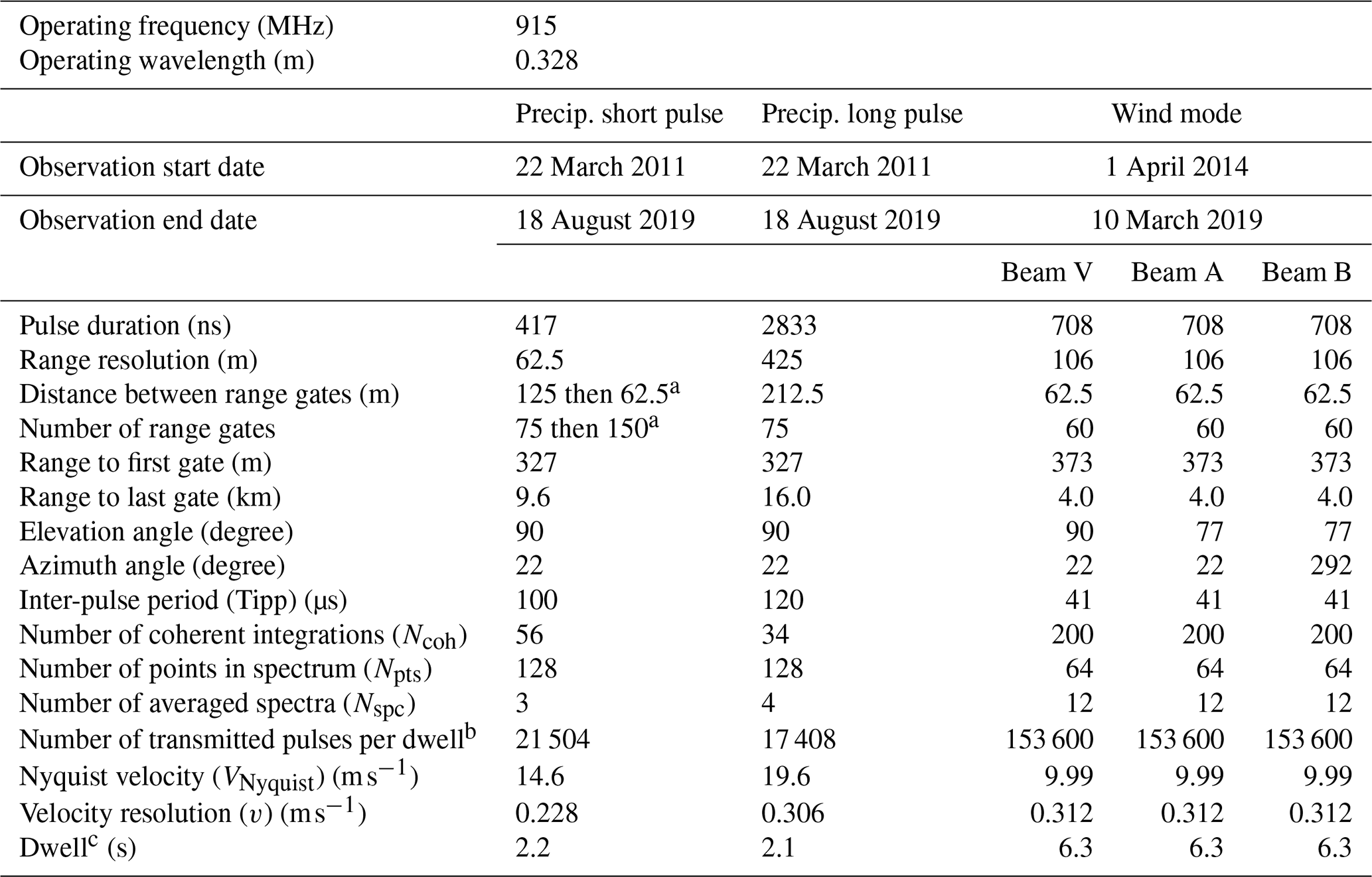
a Distance between range gates and the number of range gates changed on 4 April 2014. b Number of transmitted pulses per dwell: (NcohNnptsNspc). c Dwell is the time needed to transmit all pulses: Dwell=(TippNcohNptsNspc) (s).
2.1 Radar wind profiler
The ARM SGP Central Facility RWP was a Vaisala Meteorological Systems Inc. LAP-3000 wind profiler (Muradyan and Coulter, 2020) and is a commercial version of the NOAA UHF wind profiler developed under an industry–government 1991 Cooperative Research and Development Agreement (CRADA). From 22 March 2011 to 31 March 2014, the RWP operated in a precipitation mode observing only in the vertical direction. The precipitation mode sampled the atmosphere with a short and long pulse, yielding low-sensitivity short-range measurements and high-sensitivity long-range measurements, respectively. On 1 April 2014, a wind mode was added to the RWP and consisted of transmitting pulses in three different directions in order to estimate the horizontal wind as a function of height. The RWP collected data in both precipitation and wind modes for 5 years. On 11 March 2019, the wind mode operating parameters changed, and on 19 August 2019, the RWP hardware failed and was eventually replaced with a wind profiler produced by a different radar manufacturer. The LAP-3000 RWP can only collect data in one beam direction with one pulse configuration at a time. Thus, during the 2011 to 2014 period, the radar alternated between two vertically pointing precipitation mode radar beams, requiring approximately 5 s to collect both beams of data. During the 2014 to 2019 period, the radar sequentially collected data in five unique radar beams (i.e. two precipitation mode beams and three wind mode beams), requiring approximately 25 s to complete one observation cycle. Table 1 lists pertinent RWP operating parameters for both modes.
The ARM RWP uses the manufacturer's default processing routines (Muradyan and Coulter, 2020). For each mode, the RWP transmits a sequence of pulses and performs coherent integrations, fast Fourier transforms (FFTs), and spectra averages. Using the precipitation short-pulse mode as an example, the RWP transmits 56 radar pulses (represented by Ncoh) and integrates the in-phase and quadrature voltages (also called I and Q voltages) to produce one in-phase and one quadrature voltage (i.e. Icoh and Qcoh). After collecting 128 (represented by Npts) coherently averaged Icoh and Qcoh voltages, a von Hann window is applied to the time series and a complex FFT is performed to produce a Doppler velocity power spectrum. Another sequence of 7168 pulses (calculated as NcohNnpts) is transmitted and processed to produce another Doppler velocity power spectrum. After producing three power spectra (represented by Nspc), the three power spectra are averaged and saved to disc. The option of calculating a median spectrum or statistically averaging the three spectra (as discussed in Merritt, 1995) in order to remove transient signals (e.g. birds or other flying objects passing through the radar beam) was not implemented. A total of 21 504 pulses (NcohNptsNspc) are transmitted per dwell and a 100 µs inter-pulse period yields a 2.2 s dwell. For each Doppler velocity spectrum, the first three spectrum moments (i.e. signal-to-noise ratio, mean radial velocity, and spectrum width) are estimated using the manufacturer's single peak processing routine with integration limits bounded by the Nyquist velocities ± VNyquist. The average spectra and the moments are saved to disc.
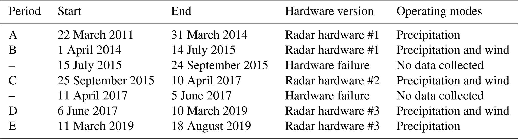
Between 2011 and 2019, the RWP had two hardware failures. In 2015, the phase shifter module controlling the beam-pointing direction failed due to age and overuse. A new phase shifter module was installed. In 2017, the final amplifier in the transmitter module failed, and several relays failed in the phase shifter module. The transmitter module was replaced with a used Vaisala unit scavenged from a newer RWP, and the relays were replaced. Since calibration constants change with ageing and changing hardware, the RWP dataset is divided into five calibration periods as listed in Table 2.
2.2 Surface disdrometer
A 2-dimensional video disdrometer (VDIS) manufactured by Joanneum Research in Graz, Austria (Schönhuber et al., 2008), was deployed about 100 m from the RWP at the SGP Central Facility (Wang et al., 2021; ARM, 2011). The VDIS uses two orthogonal pointing cameras in the horizontal plane to detect raindrops falling through a 10 cm square opening and then estimates the raindrop number concentration with a 1 min temporal resolution (Tokay et al., 2001, 2013). Radar reflectivity factors assuming Rayleigh scattering were calculated using PyDisdrometer routines (Hardin and Guy, 2014), as used in previous studies using VDIS observations (Giangrande et al., 2019).
The calibration procedure uses the 1 min surface disdrometer radar reflectivity factor to estimate a RWP calibration constant for the precipitation short-pulse mode using 1 min averaged RWP observations at 500 m altitude. The other RWP modes could be calibrated directly with the 1 min surface disdrometer observations, but to increase the number of samples, the other RWP modes are calibrated using the precipitation short-pulse mode as a reference and using multiple range gates and nearest-in-time observations. The calibration procedure described herein is only valid for RWP modes that collect data while it is raining. If the RWP is adaptive and collects precipitation mode data when it is raining and wind mode data otherwise, then there are not any nearest-in-time precipitation mode observations nor surface disdrometer observations available to calibrate the wind mode observations. In this situation, the precipitation mode data can be calibrated, but the wind mode data cannot be calibrated with the disdrometer observations.
The ARM RWP records the average Doppler velocity power spectra, and real-time spectrum moments are calculated on the RWP host computer using the RWP manufacturer processing routines. These real-time spectrum moments are labelled “a0” using ARM's file naming protocols (ARM, 2022) and saved on the ARM archive in netCDF format (ARM 1998a, b, c, d). The recorded spectrum moments are not calibrated and do not include a radar reflectivity factor estimate. To illustrate the motivation for reprocessing the recorded spectra and recalculating the spectrum moments, Fig. 1 shows time–height cross-sections of recorded moments including signal-to-noise ratio (SNRa0) (dB) (Fig. 1a), mean radial velocity () (m s−1) (Fig. 1b), and spectrum noise power () (dB) (Fig. 1c) for a rain event on 7 June 2018 using the precipitation short-pulse mode. Examination of the SNRa0 time–height structure in Fig. 1a suggests convective rain near 11:45 to 12:00 UTC, followed by stratiform rain after about 12:15 UTC. There are a couple questionable features in this figure between 11:35 and 12:10 UTC that raise concern about the quality of the real-time spectrum moments. First, the SNRa0 contains speckles of low-magnitude SNR above the height of about 3 km. Second, the has large, unphysical jumps in velocity over several range gates and over several profiles due to Nyquist velocity aliasing. Third, the spectrum noise power , which is the denominator in estimating SNR, has large and variable magnitudes at nearly all range gates. The first two features are due to the online processing codes incorrectly estimating the spectrum moments, and the third feature is due to the broad signal velocity power spectra occupying a large portion of the velocity power spectrum, causing the noise level estimate to be contaminated by the signal power.
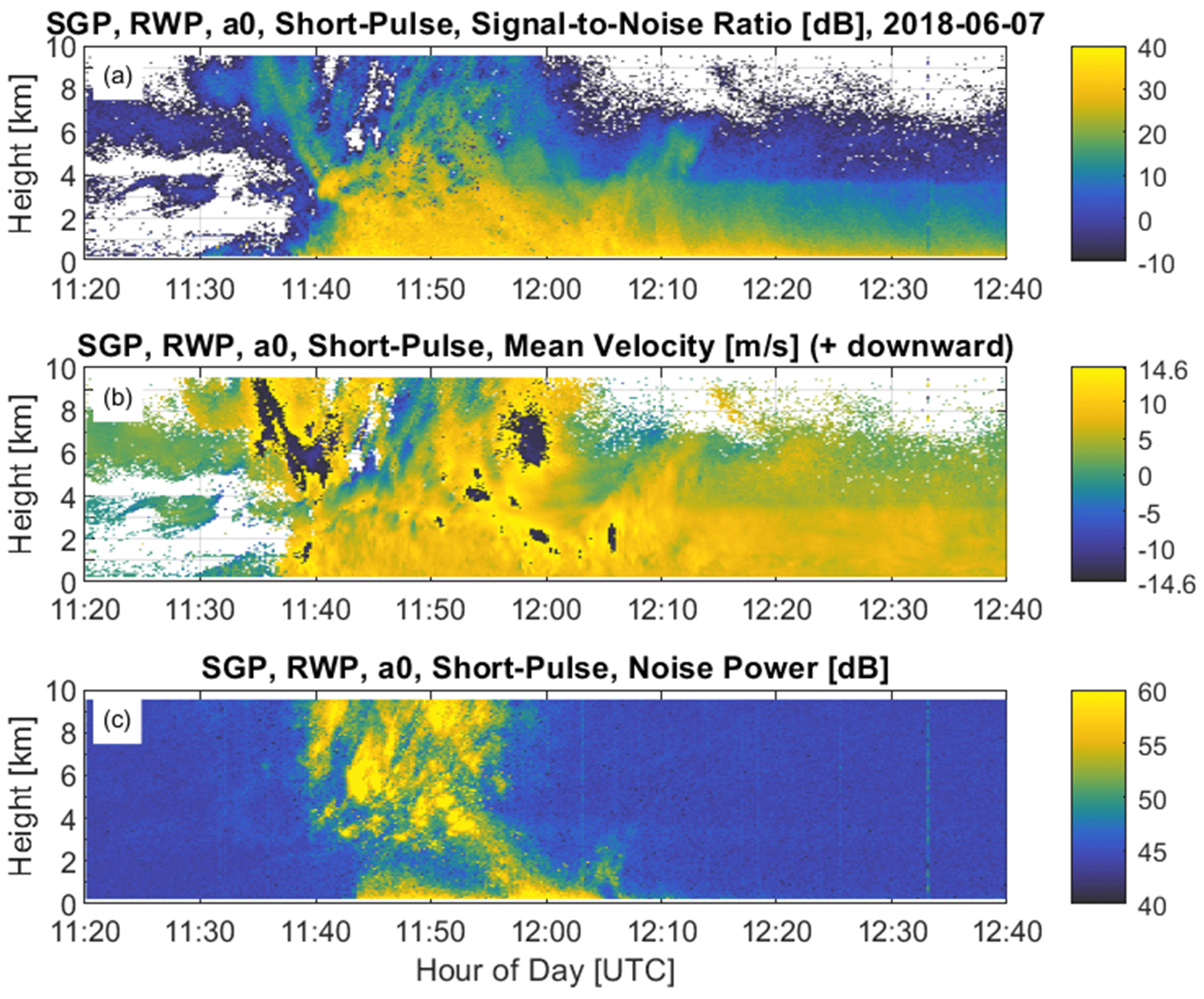
Figure 1Radar wind profiler (RWP) spectrum moments calculated with the real-time processing algorithms and downloaded from the DOE ARM archive. RWP is located at the SGP Central Facility. Observations are from the vertically pointing beam using the precipitation short-pulse mode on 7 June 2018 between 11:20 and 12:40 UTC. (a) Signal-to-noise ratio (SNR) (dB), (b) mean radial velocity with positive values moving downward toward the radar (m s−1), and (c) spectrum noise power (dB).
This section describes the five-step RWP calibration procedure. First, the raw Doppler velocity power spectra are adjusted to account for both Nyquist velocity aliasing (see Sect. 3.1.1) and coherent integration filtering (see Sect. 3.1.2). Second, the spectrum moments are recalculated (see Sect. 3.1.3). Third, the recalculated SNR is increased to account for leaking signal power into the noise power to yield an adjusted signal-to-noise ratio (see Sect. 3.2). Fourth, a calibration constant is determined for the precipitation short-pulse radar beam (defined as the “reference” beam) by comparing radar reflectivity factors with surface disdrometer observations (see Sect. 3.3). The last step determines relative calibration offsets between the reference beam and the other four radar beams. The calibration constant for each beam is the combination of the reference beam calibration constant and that beam's relative calibration offset (see Sect. 3.4). To differentiate between the real-time processed moments and the reprocessed moments, the former estimates are labelled “a0” and the latter are labelled “revised”.
3.1 Doppler velocity power spectrum adjustments and calculating spectrum moments
This subsection describes three processing steps: (1) spectrum adjustments due to Nyquist velocity aliasing, (2) spectrum adjustments due to coherent integration, and (3) recalculating the spectrum moments. Appendix A presents a flow diagram illustrating how these processing steps are applied to a profile of radar observations.
3.1.1 Eliminating Nyquist velocity aliasing
Nyquist velocity aliasing is when the target radial velocity exceeds the Nyquist velocity, and the target appears to be moving in the opposite direction. One velocity aliasing mitigation technique is to concatenate two copies of the same Doppler velocity spectrum to remove the artificial boundary at the Nyquist velocity (Williams et al., 2018). Figure 2 shows an example of velocity aliasing between 5 and 8 km using precipitation short-pulse mode Doppler velocity power spectra for a single profile collected on 7 June 2018 at 11:58:20 UTC. The original power spectra are plotted within the Nyquist velocity (VNyquist) range of ± 14.6 m s−1, with downward motions having positive values consistent with raindrop gravitational fall speeds. The original spectra are copied in Fig. 2 to visualize and to mitigate Nyquist velocity aliasing. Specifically, the original downward motions between 0 and 14.6 m s−1 are copied to upward motions between −29.2 and −14.6 m s−1. The original upward motions between −14.6 and 0 m s−1 are copied to downward motions between 14.6 and 29.2 m s−1. The red circles in Fig. 2 designate real-time mean radial velocity moments . Note the jump in near 5.5 km from downward to upward motion, which is due to the assumption in the real-time signal processing routines that all signal power is within the Nyquist interval of ±VNyquist.
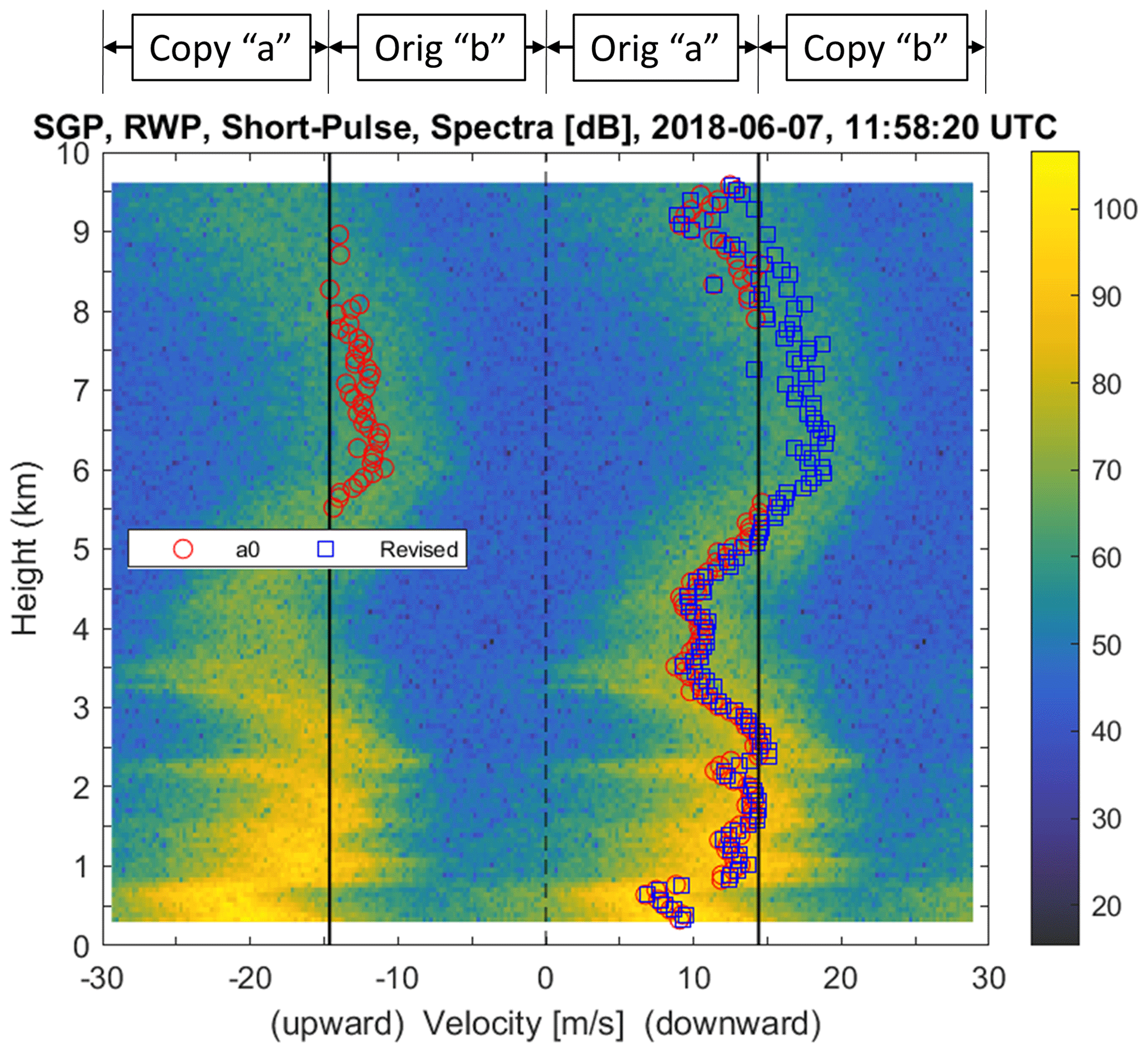
Figure 2Spectra profile at time 11:58:20 UTC on 7 June 2018. Downward velocities have positive values and are approaching the ground-based radar. Original spectra are plotted between Nyquist velocities −14.6 and 14.6 m s−1 and are indicated with solid lines. The portion of original spectra with downward motion is copied to be more upward than the Nyquist velocity (i.e. portion labelled “a”), and the portion of original spectra with upward motion is copied to be more downward than the Nyquist velocity (i.e. portion labelled “b”). Red circles designate real-time estimated mean radial velocities, and blue squares denote revised mean radial velocities. Dashed line indicates 0 m s−1 velocities. Spectra magnitudes are uncalibrated spectral power density units expressed in decibels (i.e. 10log[S(v)] with units dB).
For spectra that have velocity aliasing, the SNR is biased low when using the assumption that all of the signal power is within ± VNyquist. This issue can be visualized in Fig. 3 and shows individual spectra at 6 km (Fig. 3a) and 3 km (Fig. 3b). The signal-to-noise ratio can be estimated using (Riddle et al., 2012):
where vstart and vend (m s−1) are the integration limits indicating the start and end velocities of the power spectrum S(vi) containing signal power (uncalibrated power per (m s−1)), vi is the velocity bin, Δv (m s−1) is the velocity bin resolution, is the spectrum mean noise level (uncalibrated power per (m s−1)) (Hildebrand and Sekhon, 1974), and Npts is the number of points in the spectrum. The real-time processing routine uses only the spectrum between ± VNyquist to determine the spectrum moments. In Fig. 3b, the maximum magnitude is near 10 m s−1 (downward), the vstart integration limit is near 0 m s−1, and the vend limit stops at the Nyquist velocity of 14.6 m s−1. The spectrum between these integration limits is shaded red and labelled a0 spectrum in Fig. 3. The revised processing routine uses the extended spectrum that spans between ± 2VNyquist. Since the original spectrum is copied into the extended spectrum, the maximum magnitude peak that occurs near 10 m s−1 (downward) also occurs near −19 m s−1 (upward). The revised processing routine uses information from the previous range gate to select which of the two peaks to process. Appendix A describes the processing steps using a prior velocity Vprior to select one of the two peaks. After a peak is selected, the revised processing routine uses the same search technique as the real-time processing routine, except it uses the extended spectrum illustrated in Figs. 2 and 3. For the spectrum shown in Fig. 3b, the vstart integration limit is the same determined from the real-time processing routine, but the vend limit extends past the Nyquist velocity and ends where the spectrum crosses the mean noise level near 20 m s−1 (downward). The different integration limits cause the real-time processing method to underestimate both the SNR and mean radial velocity relative to the dealiased method by 0.2 dB and 0.2 m s−1, respectively. As will be seen in the next section, including the incoherent averaging filtering effects will increase these differences.
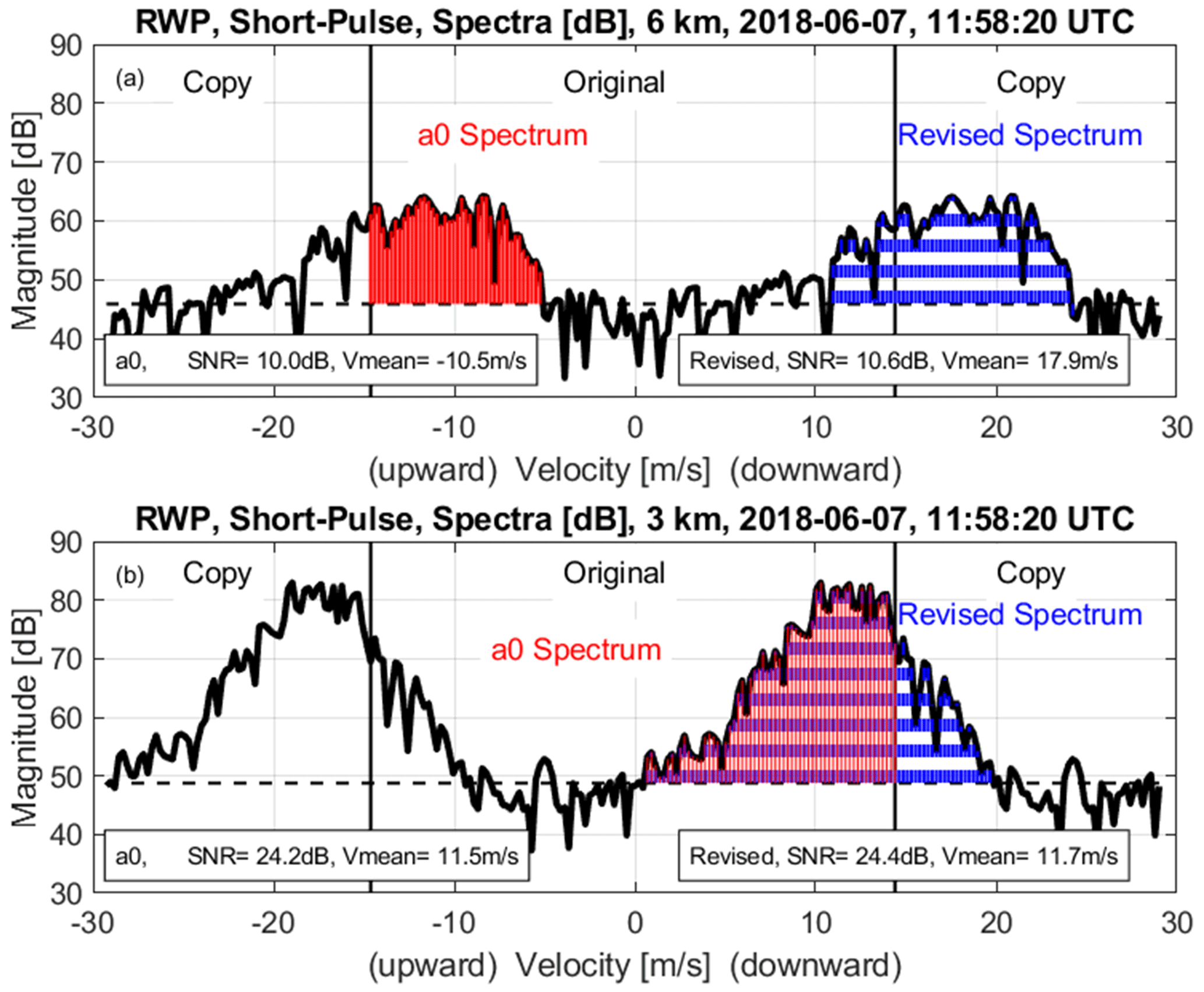
Figure 3Example of integration limits used in the real-time and revised spectrum moment estimation algorithms. Uncalibrated spectral power density expressed in decibels (dB) for profile at 11:58:20 UTC on 7 June 2018 at (a) 6 km and (b) 3 km. Red shading and horizontal blue bars indicate spectral power density used to estimate a0 and revised moments, respectively.
In Fig. 2, between 5.5 and 9 km, appears to have upward motion. This is because the true maximum spectrum magnitude has a downward velocity occurring outside the ± VNyquist boundaries, and the aliased peak has an upward velocity. Figure 3a shows the velocity power spectrum at 6 km, and the real-time processing routine found integration limits that bound the upward spectrum maximum magnitude peak near −12 m s−1. The integration limits are −14.6 (at the Nyquist boundary) and approximately −5 m s−1. This a0 spectrum region is shaded red in Fig. 3a. In contrast, the revised processing routine selected the downward moving peak in the dealiased spectrum and found integration limits of approximately 11 and 24 m s−1 downward (spectrum region with blue strips). The different integration limits produce significantly different mean radial velocities of equal to −10.5 m s−1 and equal to 17.9 m s−1.
3.1.2 Coherent integration adjustment
Coherent integration is a signal processing technique that accumulates the radar measured in-phase and quadrature voltages (a.k.a. I and Q voltages) over consecutive transmitted pulses. Sinusoidal oscillations with slowly varying phase over the accumulation interval are said to be coherent, and their accumulated I and Q voltages cause an increase in signal power. Conversely, accumulating I and Q voltages over high-frequency oscillations, including noise fluctuations, will produce lower-magnitude accumulated I and Q voltages resulting in smaller signal power. Thus, coherent integration increases radar detection by acting as a low-pass filter that increases low-frequency signal powers and decreases high-frequency noise power (Farley, 1985).
Coherent integration is also known as time-domain averaging (TDA) and is implemented by changing the number of coherent integration samples Ncoh, which changes the effective time between transmitted samples and decreases the Nyquist velocity using
where λ is the radar operating wavelength and TIPP is the inter-pulse period (a.k.a. time between transmitted pulses). Coherent integration also applies a boxcar filter to the I and Q voltage time-series samples before integrating, which is equivalent to applying a low-pass filter to the integrated time series (Wilfong et al., 1999). Since coherent integration is performed before computing the FFT on the complex I and Q voltage samples, the low-pass filter manifests as a reduction in FFT signal power magnitude as a function of velocity vi and has the form (Schmidt et al., 1979)
where ) is the recorded signal power spectrum at velocity bin vi, ) is the expected signal power spectrum without any time-domain low-pass filtering effects, and Npts is the number of complex I and Q samples after coherent integration, which is also the number of velocity bins in the power spectrum after performing the FFT calculation. The ratio yields integers from to . Note that the low-pass filter response function (the expression within the square brackets in Eq. 3) has a magnitude of one when vi=0 and decreases with increasing vi.
The impact of the TDA low-pass filter can be mitigated by applying a correction factor to the recorded Doppler velocity power spectra, as discussed in Wilfong et al. (1999). Since the low-pass filter only affects coherent signals, the correction factor should only be applied to the signal portion of the power spectrum and not to the random noise power. Thus, the TDA-corrected power spectrum STDA(vi) is estimated using
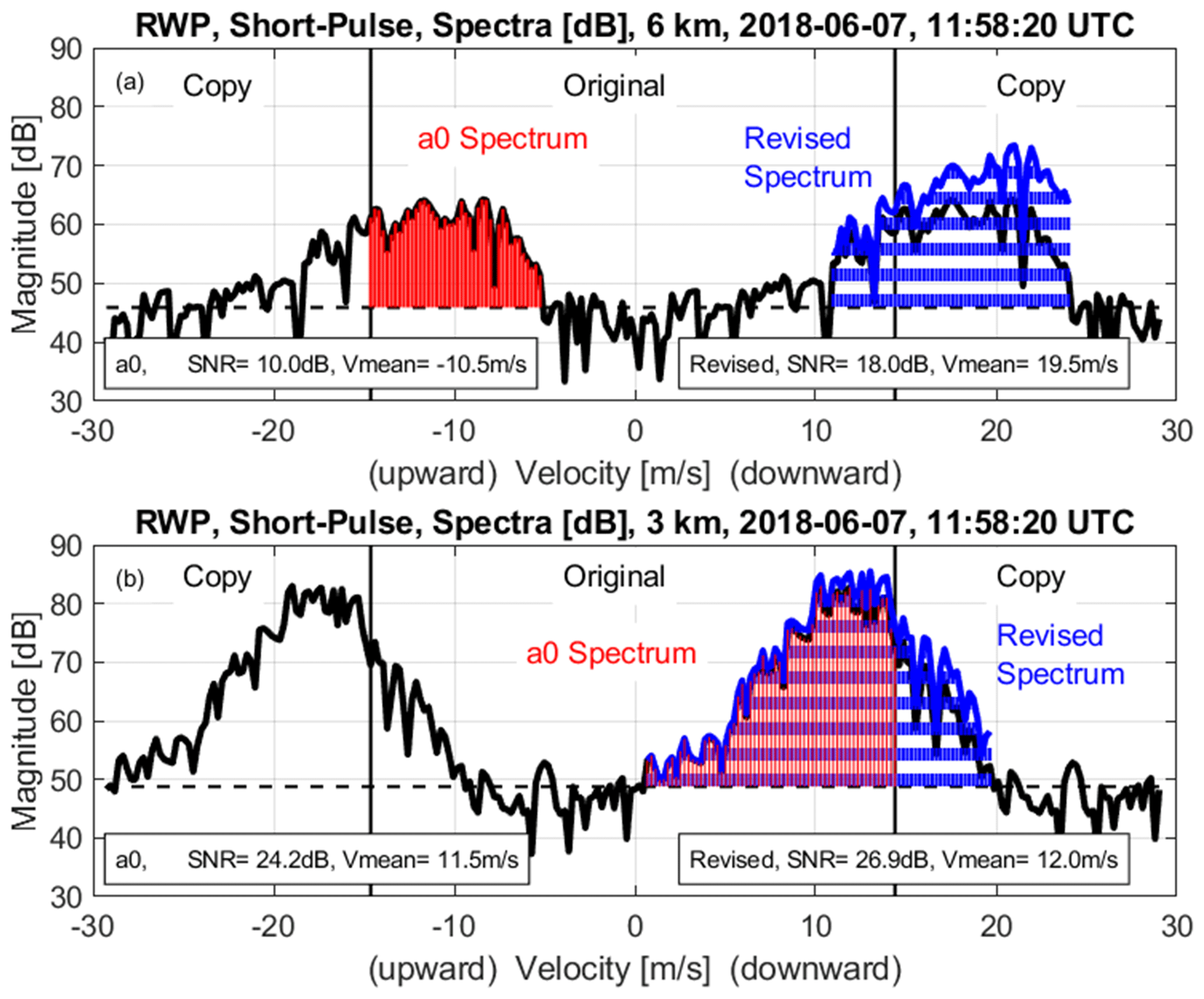
where S(vi) is the recorded Doppler velocity power spectrum. For the precipitation short-pulse mode, the correction factor magnitude (the expression in the square brackets in Eq. 4) at ± VNyquist is 2.47 in natural units as in Eq. (4) or 3.9 dB in decibels. Figure 4 shows the recorded power spectra shown in Fig. 3, with the revised spectrum corrected for the TDA filtering expressed in Eq. (4). The SNR and mean radial velocity moments for real-time moments and the revised spectrum are listed in Fig. 4. Comparing the non-TDA- and TDA-corrected moments for the dealiased spectra at 6 km (see Figs. 3a and 4a, respectively) indicates that the SNR increased by 7.4 dB, and the mean radial velocity became more downward by 1.6 m s−1 when including the TDA filter correction. Note that the difference in a0 and TDA-corrected mean radial velocities at 6 km is 30 m s−1 (see Fig. 4a) and is not a multiple of ± 2VNyquist (± 29.2 m s−1). This indicates that simple integer ± 2VNyquist adjustments, as proposed by Tridon et al. (2013), will not account for improper integration limits used in the real-time processing routines.
3.1.3 Calculating spectrum moments
After adjusting the recorded spectrum due to Nyquist velocity aliasing and coherent integration effects, the spectrum moments are calculated following the method and equations presented in Williams et al. (2018) Appendix A. The calculated revised spectrum moments include spectrum signal power () (dB), spectrum noise power () (dB), signal-to-noise ratio (SNRrevised) (dB), spectrum mean radial velocity () (m s−1), spectrum SD (σrevised) (m s−1), spectrum width (Wrevised=2σrevised) (m s−1), spectrum skewness, and spectrum kurtosis. The dealiasing procedure described in Sect. 3.1.1 produces a spectrum with two peaks (e.g. see Figs. 2 and 3). To determine which peak to analyse, the processing routine starts at the lowest range gate and calculates a prior velocity Vprior that is used to select a peak in the next range gate. More details of the processing steps are provided in Appendix A.
3.2 Signal-to-noise ratio (SNR) adjustment
Signal power is estimated relative to the estimated mean noise power and is quantified with the signal-to-noise ratio SNR. If the noise power estimate is too large, then the signal-to-noise ratio and the inferred signal power are underestimated. The a0 processed noise power shown in Fig. 1c had increased magnitudes at nearly all range gates during the convective rain event between approximately 11:35 and 12:10 UTC. This increased noise power is not expected for RWPs because the gain is constant with range so that noise power should be independent of range. Also, Fig. 2 shows signal power spread over a large fraction of the velocity spectrum. These two features are linked: the broad signal spectra are causing increased noise power estimates. Specifically, as the signal velocity power spectrum broadens and occupies more of the velocity spectrum, the noise estimator is biased by the inclusion of signal power. The RWP online signal processing uses the Hildebrand and Sekhon (1974) noise level estimator to separate noise-only spectral bins from signal-plus-noise spectral bins based on the statistical properties of both populations (for more details see Merritt, 1995, and Wilfong et al., 1999). If the signal-plus-noise spectral bins are included in the noise-only population, then the noise level estimate will be biased high, leading to an underestimated SNR. To correct for this low SNR bias, a reference noise power (dB) is determined and an adjusted SNR is estimated using
where SNRrevised and are moments calculated in Sect. 3.1.3.
The noise power for every spectrum is estimated using the method outlined in Hildebrand and Sekhon (1974). The reference noise power is the median noise power derived from all spectra collected on a given day. Figure 5 shows the daily median noise power for the precipitation short pulse (black plusses) and long pulse (red crosses) for the 8-year dataset. The jump in daily median noise power in mid-2017 corresponds to replacing the transmitter with a used, yet updated version, from the same RWP vendor. It is interesting to note that the seasonal noise variation decreased with the updated transmitter and not when the equipment shelter air conditioning system was updated in mid-2016.
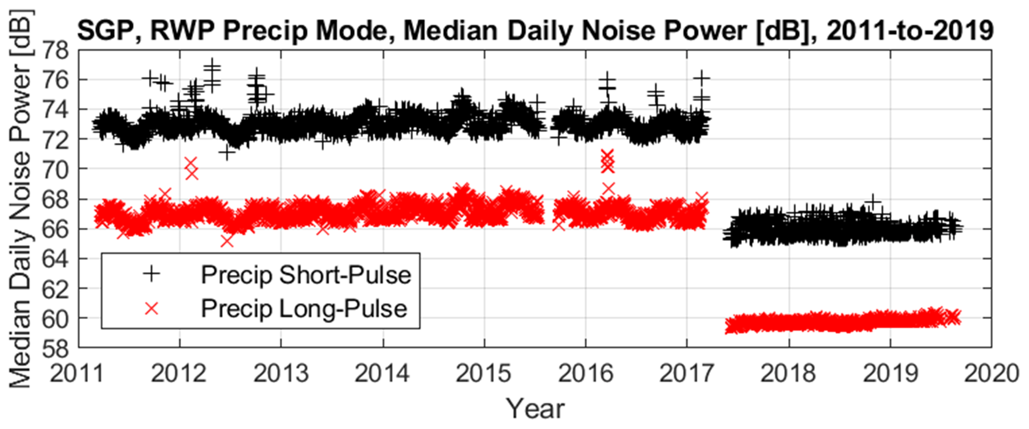
Figure 5Daily median noise level for the precipitation short-pulse (black plusses) and long-pulse (red crosses) mode for observations between 2011 and 2019.
Figure 6 illustrates the impact of adjusting the signal-to-noise ratio with the reference noise power. Figure 6a shows the real-time estimated SNRa0 (thick line) and (thin line) profiles. The large variations in between 4 and 5 km appear as large and inverse variations in SNRa0. Figure 6b shows the adjusted signal-to-noise ratio using two methods. The method described in Tridon et al. (2013) uses the real-time moments (SNRa0 and ) to estimate the adjusted signal-to-noise ratio (thick blue line in Fig. 6b). The method described herein recalculates the moments and then estimates the adjusted signal-to-noise ratio using Eq. (5) (thin red line). The profile offset in Fig. 6b is due to different reference noise powers used in the two methods. The has more variability than , indicating that the revised spectra reprocessing method produces smoother, more vertically consistent SNR vertical profiles than the Tridon et al. (2013) method.
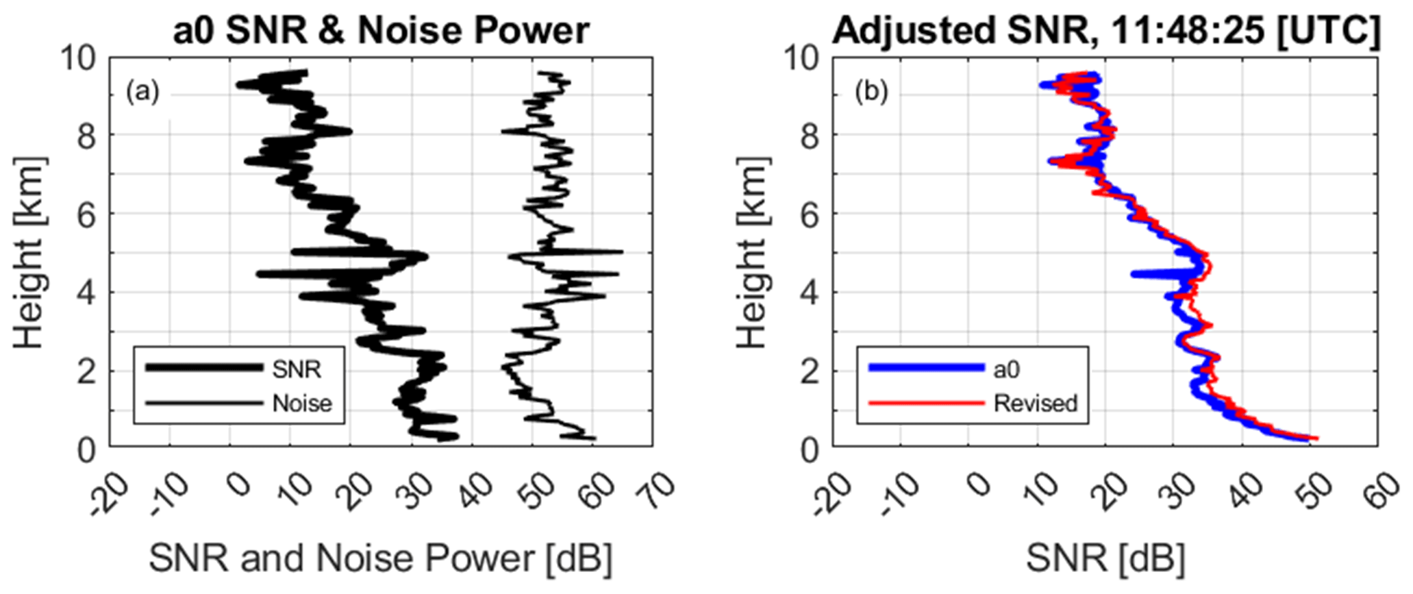
Figure 6Moment profiles at time 11:48:25 UTC on 7 June 2018. (a) SNR and spectrum noise power from real-time spectrum processing routines. (b) Adjusted SNR using the a0 moments shown in panel (a) (thick blue line) and adjusted SNR using the revised spectral method (thin red line). The adjusted SNR profiles are offset because of different reference noise values.
3.3 Calibrating reference beam to surface disdrometer
The precipitation short-pulse beam is defined as the RWP reference beam, and the radar reflectivity factor ZPrecipShort (dBZ) for this beam is estimated from the adjusted signal-to-noise ratio using
where r (m) is range from the radar, and CPrecipShort (dB) is the calibration constant. To estimate the calibration constant CPrecipShort, an initial value of CPrecipShort equal to 0 dB is selected, and Eq. (6) is used to estimate the RWP reflectivity factor at all range gates. These initial RWP reflectivity factors at 500 are averaged into 1 min quantities and then compared with the 1 min surface disdrometer radar reflectivity factors. Using only disdrometer reflectivity factors between 20 and 40 dBZ, the reflectivity factor differences are calculated for RWP lags between ± 4 min. Both positive and negative lags are needed because the two instruments are separated by approximately 100 m, and the horizontal wind speed and direction can cause the surface rain observations to occur before the radar observations at 500 m altitude. Figure 7 shows scatter plots and statistics of mean, SD, and Pearson's correlation coefficient for the 7 June 2018 rain event at nine different lags. For this rain event, the distribution in Fig. 7d is selected for calibration because it has the highest Pearson's correlation coefficient of 0.95.

Figure 7Scatter plots of reflectivity factor differences between RWP precipitation short-pulse mode (with CPrecipShort = 0 dB) and surface disdrometer for different minute lags for the rain event on 7 June 2018. Positive lags indicate RWP shifted to a later time. Lag times for each panel are (a) −4 min, (b) −3 min, (c) −2 min, (d) −1 min, (e) 0 min, (f) 1 min, (g) 2 min, (h) 3 min, and (i) 4 min. This rain event had 153 min samples with surface disdrometer reflectivity factor between 20 and 40 dBZ. Each panel indicates rain event mean difference, standard deviation (SD), and Pearson's correlation coefficient (r). Panel (d) has the largest Pearson's correlation coefficient and is used for calibrating this event. The calibration constant for this event is CPrecipShort = −49 dB.
Using the calibration constant and lag determined from Fig. 7d (i.e. CPrecipShort = −49.5 dB and −1 min lag), Fig. 8a shows the time–height cross-section of calibrated RWP precipitation short-pulse mode radar reflectivity factor. Figure 8b shows a time series of RWP reflectivity factor at 500 m (red crosses) and the surface disdrometer reflectivity factor (black plusses). The thin blue lines in Fig. 8b at 20 and 40 dBZ indicate the reflectivity factor range used for calculating the RWP and disdrometer differences, which are shown in Fig. 8c. Also shown in Fig. 8c are the statistics for this lag, including lag, number of samples, calibration constant, SD, and Pearson's correlation coefficient. Figure 8d shows surface disdrometer rain rate RR and mass-weighted mean diameter Dm. The SD of 1.9 dB for this event is due to spatiotemporal mismatch between the surface disdrometer and radar sample volume as well as measurement uncertainties of both instruments and is comparable to 1 to 2 dB measurement uncertainties of side-by-side surface disdrometers (Tapiador et al., 2017; Wang et al., 2021). Note that the lag is only used in the calibration procedure and not used as a time offset for any other purpose.
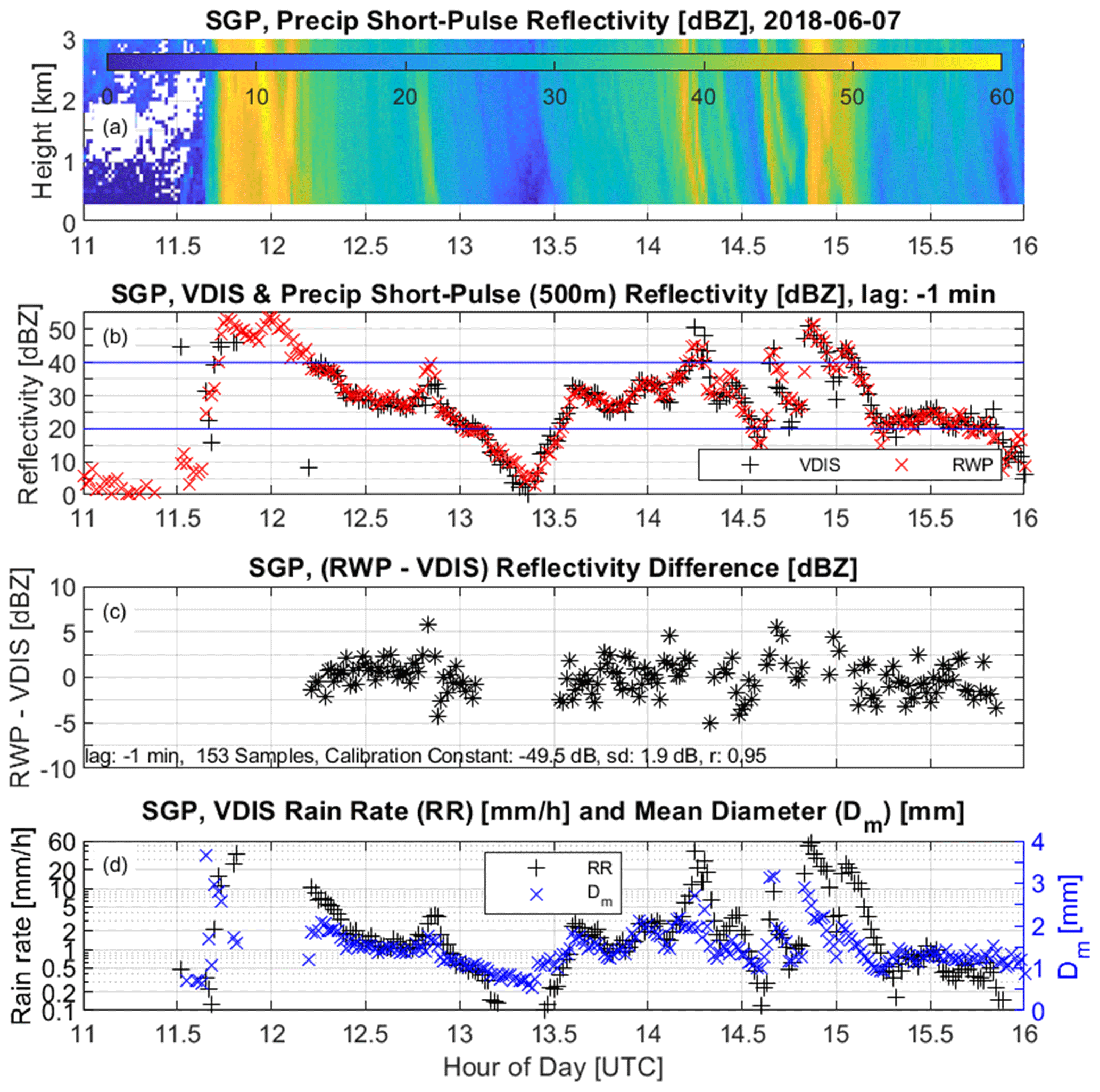
Figure 8RWP precipitation short-pulse mode and surface disdrometer observations from 7 June 2018 between 11:00 and 16:00 UTC. (a) RWP radar reflectivity factor with calibration constant of −49.5 dB; (b) RWP radar reflectivity factor (red crosses) at 500 m range with −1 min lag and surface VDIS radar reflectivity factor (black plusses); (c) reflectivity factor difference (RWP – VDIS) for samples with VDIS reflectivity factor within 20 to 40 dBZ, as indicated with blue thin lines in panel (b); and (d) disdrometer rain rate RR and mean diameter Dm. Statistics of lag, number of samples, calibration constant, standard deviation (SD), and Pearson's correlation coefficient (r) are shown in panel (c).
Figure 9 shows improved moments and calibrated reflectivity factors for the same rain event shown in Fig. 1. The top panel (Fig. 9a) shows the revised adjusted signal-to-noise ratio (), and the middle panel (Fig. 9b) shows the revised mean radial velocity (). Compared to the a0 real-time processed moments, the reprocessed moments in Fig. 9a and b show improved data quality and uniformity. The calibrated radar reflectivity is shown in Fig. 9c.
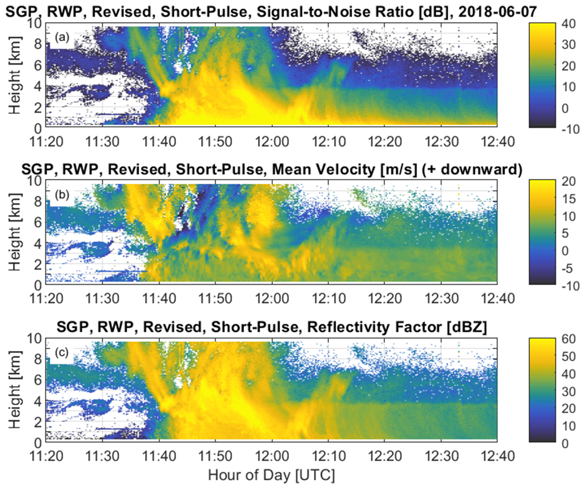
Figure 9Similar to Fig. 1 except RWP spectrum moments for the precipitation short-pulse mode calculated with the revised processing algorithms. (a) Signal-to-noise ratio (dB), (b) mean radial velocity (m s−1) with positive values moving downward consistent with raindrop gravitation fall speeds, and (c) surface disdrometer calibrated radar reflectivity factor ZPrecipShort (dBZ).
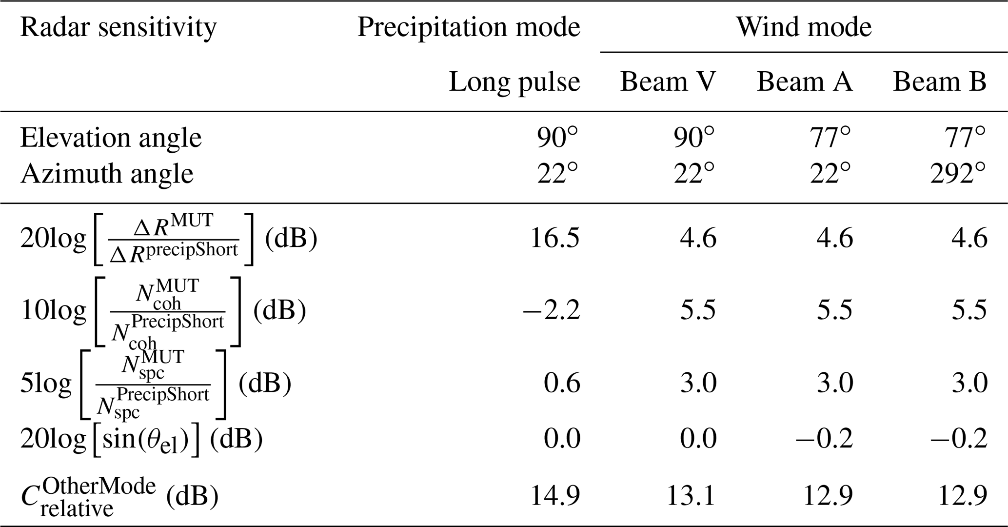
Table 3Expected relative sensitivity of other radar beams compared with the reference precipitation short-pulse beam. Relative sensitivity has four terms in Eq. (7) and is dependent on range resolution ΔR, coherent integration Ncoh, number of averaged Doppler velocity power spectra Nspc, and elevation angle.
3.4 Relative calibration constants for other radar beams
The radar sensitivity can be adjusted by changing the transmitted pulse length, the number of coherent integrations, and the number of averaged Doppler velocity spectra. Using the precipitation short-pulse mode as the reference beam, the expected relative change in sensitivity for the other four radar beams can be estimated using
where ΔR is the range resolution, Ncoh is the number of coherent samples, Nspc is the number of averaged power spectra, θel is the elevation angle from the horizon, and the superscripts PrecipShort and MUT represent the precipitation short-pulse mode and the mode under test (MUT), respectively. Using the values from Table 1 and Eq. (7), Table 3 lists the expected relative sensitivities for the precipitation long-pulse mode and the wind mode. The last term in Eq. (7) represents the decrease in gain associated with beam-pointing direction in phased-array antennas (Balanis, 1997). As the beam-pointing direction deviates from broadside (a.k.a. vertical direction in the RWP), the projected antenna area decreases, causing the gain to decrease and beam width to increase (Balanis, 1997; Palmer et al., 2022). System losses and variations in antenna gain cause the measured relative sensitivities to deviate from the expected values listed in Table 3.
The reflectivity factor for the other four radar beams follows Eq. (6) with the addition of the relative calibration constant (dB) and is estimated using
The negative sign in the bracketed term is because a positive indicates that this mode is more sensitive than the precipitation short-pulse mode and will produce a larger for the same radar reflectivity factor. Note that weaker radar reflectivity factors will be detected at further ranges at the expense of possible receiver saturation from large reflectivity factor targets at close range.
To estimate relative sensitivities between the other beams and the reference beam, reflectivity factors are estimated at all profiles and range gates using Eq. (8) with set to zero and then estimating the differences from nearby precipitation short-pulse mode observations. Figure 10 shows scatter plots and histograms of reflectivity factor differences for the precipitation long-pulse beam during the 7 June 2018 rain event. Valid observations are constrained to be within the height interval of 800 and 2100 m and precipitation short-pulse reflectivity factors greater than 30 dBZ. Over 13 000 valid samples are used from this event to calibrate the precipitation long-pulse beam. The mean relative offset is 15.5 dB for this event, with a SD of 1.3 dB. The relative calibration constant is set to 15.5 dB and implies that the long-pulse mode is more sensitive and produces a larger signal-to-noise ratio for the same radar reflectivity factor as expressed in Eq. (8).
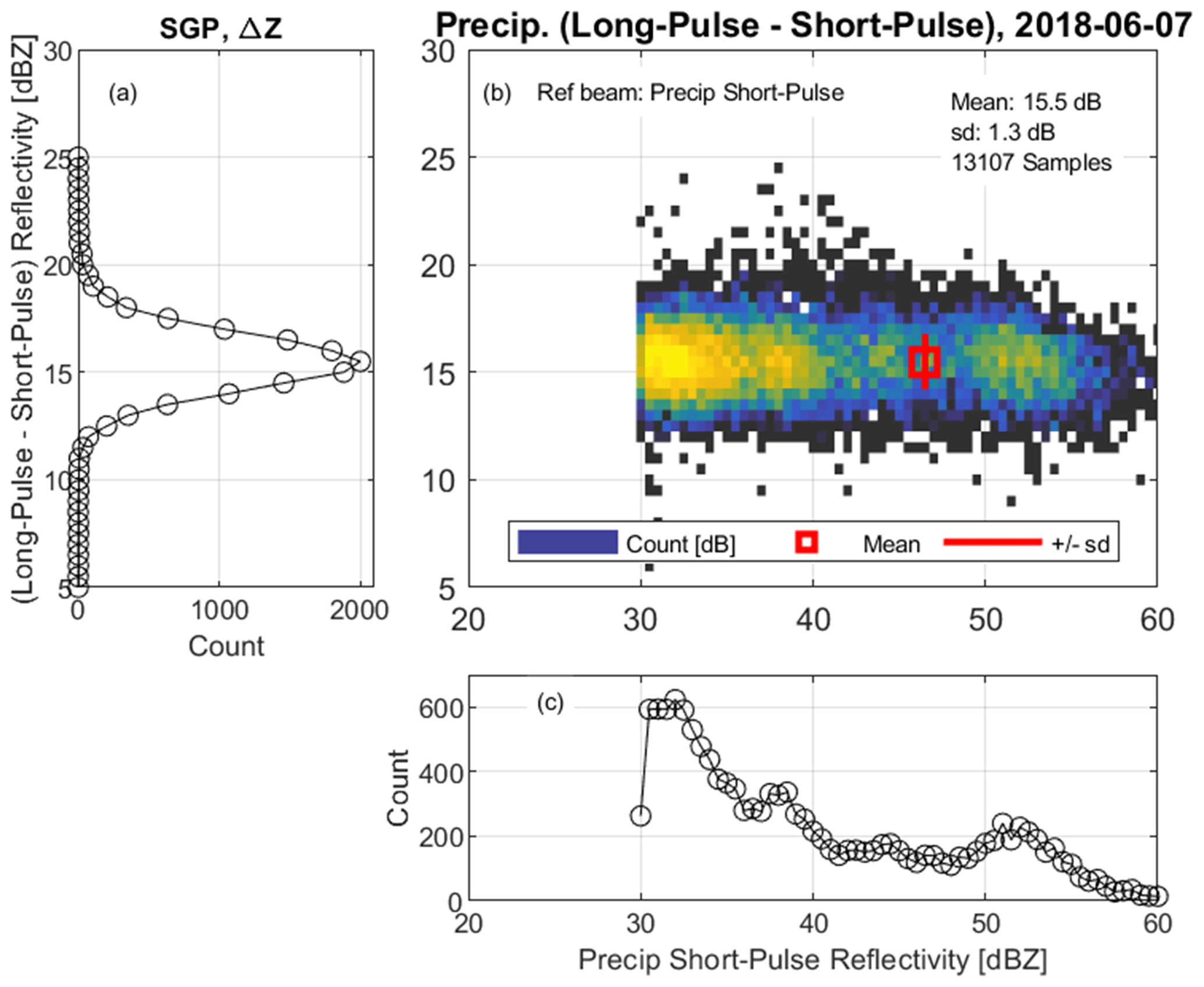
Figure 10Reflectivity factor differences between precipitation long-pulse beam with (dB) and disdrometer calibrated precipitation short-pulse beam observations for the rain event on 7 June 2018. Observations are limited to heights between 800 and 2100 m and precipitation short-pulse beam reflectivity greater than 30 dBZ. (a) Histogram of reflectivity difference (long pulse – short pulse) indicating relative calibration offset, (b) relative 2-dimensional count of reflectivity difference, and (c) histogram of disdrometer calibrated precipitation short-pulse reflectivity.
Figure 11a and b show the time–height cross-sections of cross-calibrated precipitation short- and long-pulse reflectivity factors at their native resolution for the 7 June 2018 rain event. Figure 11c shows the precipitation long-pulse relative calibration offset for each matched short- and long-pulse observation. The relative calibration offsets shown in Fig. 11c are the same samples used to produce Fig. 10 and indicate the limited height interval used in the comparison to avoid large reflectivity gradients near the radar bright band caused by melting particles.
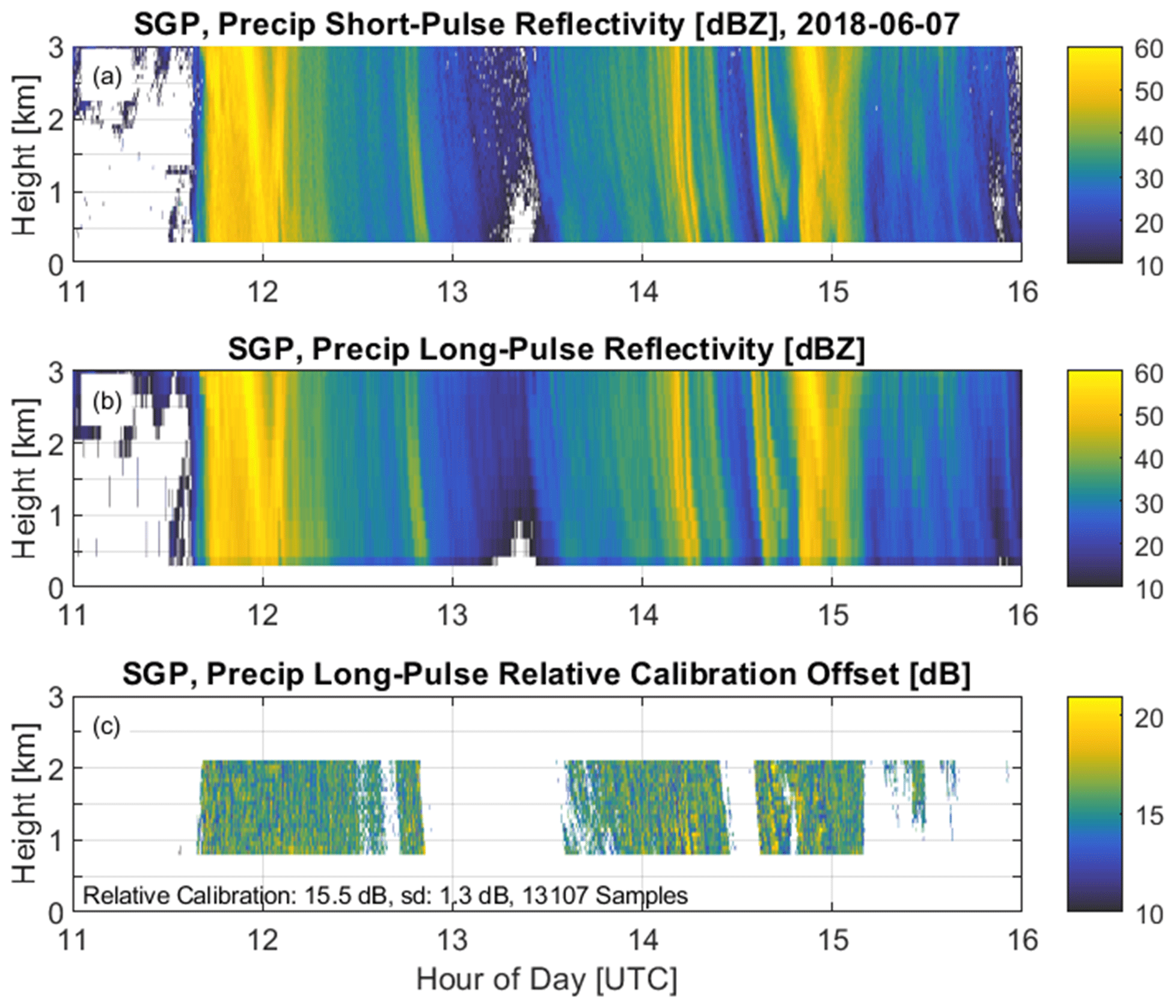
Figure 11Time–height cross-sections for the 7 June 2018 rain event. (a) Surface disdrometer calibrated precipitation short-pulse reflectivity factor ZPrecipShort, (b) cross-calibrated precipitation long-pulse reflectivity factor ZPrecipLong with = 15.5 dB, and (c) the precipitation long-pulse relative calibration offset for each matched short- and long-pulse observation. Relative calibration offset is only calculated for ZPrecipShort > 30 dBZ and for heights between 800 and 2100 m.
Estimating the relative calibration offsets for the three wind beams follows the same procedure used for estimating the precipitation long-pulse beam relative calibration offset. As expected, the calibration offsets for the oblique beams have more event-to-event variability than the vertically pointing wind mode beam and will be discussed further in the next section and shown in Fig. 14.
This section explores how the individual rain event precipitation short-pulse beam calibration constants varied over the 8-year record from 22 March 2011 to 18 August 2019. The variation of the relative calibration constants is examined as a function of ageing hardware and a function of changing radar hardware after equipment failures.
4.1 Reference beam calibration: event, monthly, and 3-month intervals
From 22 March 2011 to 18 August 2019, the precipitation short-pulse beam calibration constant CPrecipShort was estimated on 340 d, each having at least 120 min of surface disdrometer reflectivity factor greater than 20 dBZ. Figure 12 shows CPrecipShort for every valid precipitation event using black plus symbols. The calibration constant is approximately −50 dB at the beginning of this record in 2011 and then increases to about −35 dB near the beginning of 2015. There is an abrupt drop in calibration constant near the end of 2015, and then the calibration constant steadily increases until the end of this dataset in 2019. Snow events were not included in the calibration procedure.
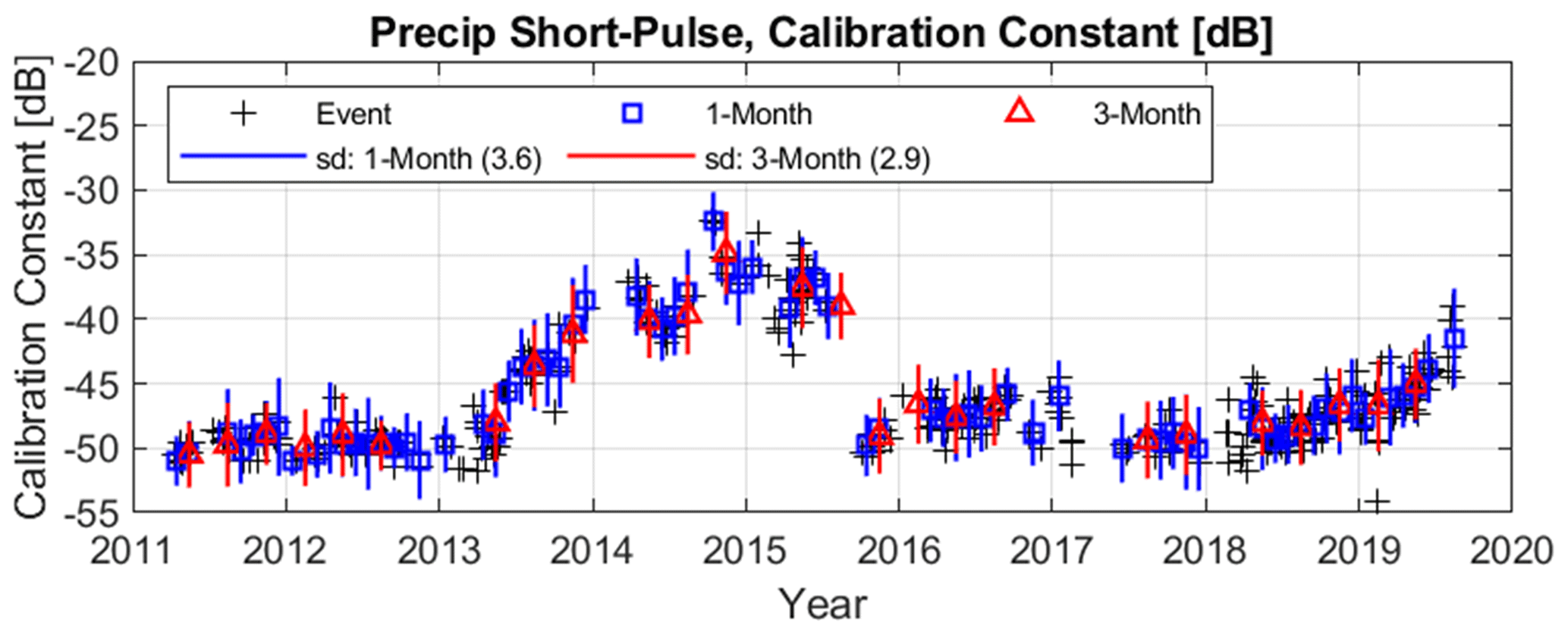
Figure 12Precipitation short-pulse beam calibration constant CPrecipShort (dB) from March 2011 through July 2019 estimated using individual rain events (black plusses), 1-month interval (blue squares), and 3-month interval (red triangles). Vertical blue and red lines are ± SD for 1- and 3-month interval calculations, respectively. Mean SDs over the 9-year dataset were 3.6 and 3.0 dB for the 1- and 3-month intervals, respectively.
An increase in calibration constant, without changing operating parameters, indicates the radar sensitivity is degrading. Referring to Eq. (6), if the reflectivity factor is constant and the measured SNR decreases because of ageing radar hardware, then the calibration constant must increase. Thus, from early 2011 to mid-2015, the calibration was stable until early 2013, then increased approximately 15 dB over the next 2 years, indicating a rapid change in calibration. There was a hardware failure in mid-2015.
The gaps in measurements in mid-2015 and early 2017 are when the radar was not operating. A new antenna phase shifter module was installed in September 2015, and the calibration constant dropped by about 10 dB relative to the old hardware. In mid-2017, a new radar transmitter and receiver module was installed, and the mean noise level dropped by about 7 dB (see Fig. 5), but the short-pulse beam calibration constant did not change significantly. The steady increase in calibration constant from 2016 through 2019 suggests an approximate 3 dB yr−1 decrease in sensitivity for this modified radar. Though not documented publicly, similar decreasing sensitivity rates have been estimated in other NOAA UHF wind profilers and have been attributed to delamination of the fibreglass patch antenna (Ecklund et al., 1988).
The slow change in calibration constant between precipitation events suggests that the disdrometer-to-RWP calibration procedure could be performed using fixed time intervals instead of individual rain events. To test this hypothesis, calibration constants were determined using all rain events during 1-month and 3-month intervals (i.e. months of JFM, AMJ, JAS, and OND). The 1- and 3-month calibration constants are plotted in Fig. 12 using blue squares and red triangles, respectively. The vertical blue and red lines represent 1- and 3-month calibration constant SDs, with mean SDs over the 9-year record equal to 3.6 and 2.9 dB, respectively. These SDs represent variations due to spatiotemporal mismatch of surface disdrometer and radar measurements, instantaneous measurement uncertainties of both instruments, and ageing hardware over the sampling interval.
4.2 Relative calibration for each hardware calibration period
Since the radar operating parameters did not change during the 2011 to 2019 interval, variations in relative calibration constants will depend on changes to the radar hardware. This section examines how the precipitation long-pulse and wind mode relative calibration constants evolved with hardware changes.
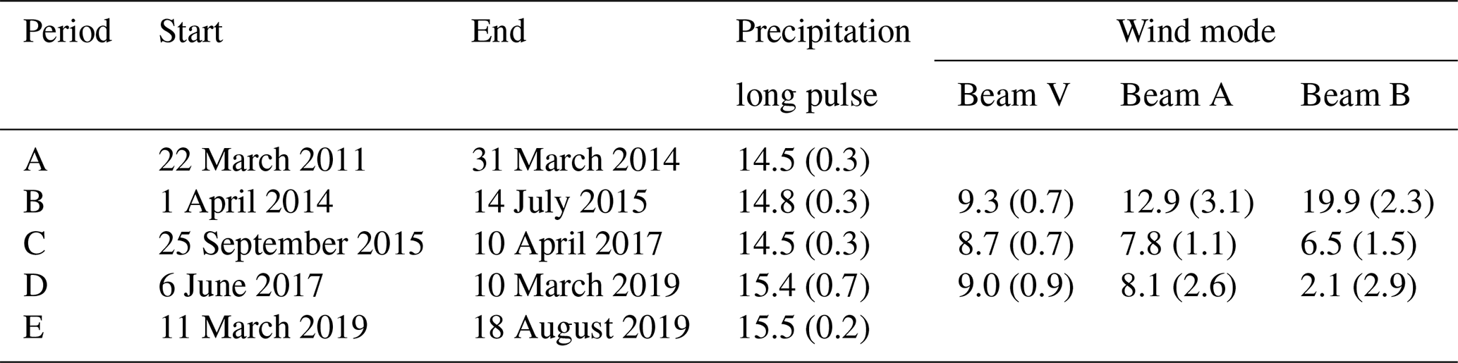
Table 4RWP relative calibration constants (dB) (SD) relative to precipitation short-pulse mode.
4.2.1 Changes in precipitation long-pulse relative calibration constants
The relative calibration constants for the precipitation long-pulse beam were estimated for every day with at least 1000 precipitation short- and long-pulse range gate samples between 800 and 2100 m range and with precipitation short-pulse reflectivity factor greater than 30 dBZ. The lower height limit of 800 m is to ensure the long-pulse beam observations are beyond the radar blind zone, and the 2100 m limit is to avoid reflectivity factor gradients near the melting layer. The precipitation long-pulse relative calibration constants were estimated for the 690 d meeting these criteria and are shown in Fig. 13 using black crosses. The dashed lines are the mean relative calibration values for each stable hardware interval labelled A through E (see Table 2). The relative calibration constant mean and SD for each interval are listed in Table 4.
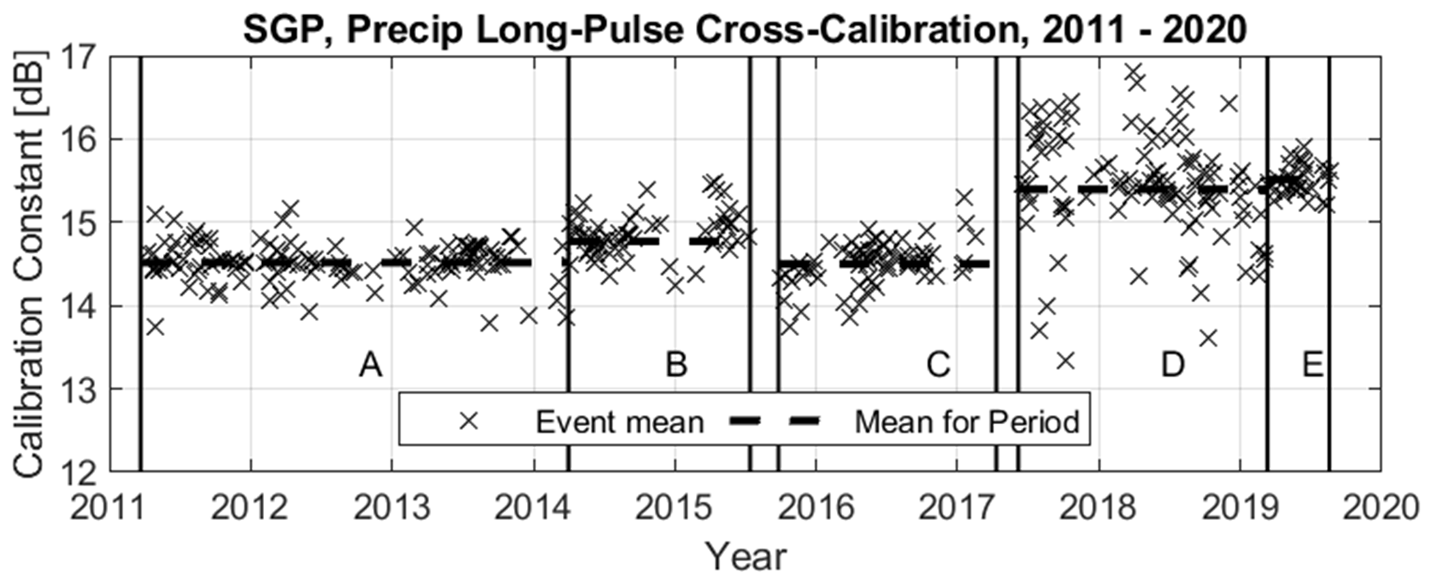
Figure 13Precipitation long-pulse beam relative calibration constant CPrecipLong (dB) from 22 March 2011 through 18 August 2019, estimated using individual rain events (black crosses). Thick dashed lines are mean relative calibration constants (listed in Table 4) for stable hardware intervals labelled A through E as described in Table 2.
4.2.2 Changes in wind mode relative calibration constants
Similar to the conditions applied when estimating the precipitation long-pulse beam relative calibration constants, the wind mode beams were estimated for every day with at least 1000 range gate samples between 500 and 2100 m range and with precipitation short-pulse reflectivity factor greater than 30 dBZ. The wind mode has a shorter pulse length than the precipitation long-pulse beam, which enables valid wind observations down to 500 m. Figure 14 shows the daily relative calibration constants for the three wind beams (black crosses), with thick dashed lines representing the mean relative calibration constant for each hardware interval. The vertical beam relative calibration constant is fairly stable over the 2014 to 2019 observation period, with values listed in Table 4. There is more event-to-event variability in the oblique beam relative calibration constants compared to the vertical beam because there is more horizontal distance between the vertical pointing reference beam and the oblique beams. A 14∘ off-vertical pointing angle causes approximately 250 m horizontal distance between the vertical beam and oblique beam at 1 km height. Aside from the larger event-to-event variability, the oblique beam mean relative calibration constants change for each radar hardware configuration. This is probably due to changes in the antenna phase shift module that controls the antenna beam pattern and pointing direction. Table 4 lists the mean oblique beam relative calibration constants for each hardware configuration.

Figure 14Relative calibration constants for wind mode for every rain event from March 2014 through February 2019. (a) Vertical beam (beam V, az: 22∘, el: 90∘), (b) oblique beam (beam A, az: 22∘, el: 76∘), and (c) oblique beam (beam B, az: 292∘, el:y76∘). The thick dashed lines are mean relative calibration constants (listed in Table 4) for stable hardware intervals labelled B, C, and D as described in Table 2.
This work describes a procedure to calibrate a UHF-band radar wind profiler (RWP) reflectivity factor to surface disdrometer observations. The revised procedure builds on the method described in Tridon et al. (2013) by correcting the recorded Doppler velocity power spectra due to Nyquist velocity aliasing and coherent integration bias effects, before recalculating the spectrum moments. The revised method also calibrates the oblique pointing RWP beams that are used to measure horizontal wind motions.
This cross-calibration procedure uses precipitation measurements from one instrument (i.e. surface disdrometer) as the reference dataset and then calibrates another instrument (i.e. the RWP) using measurements from the same precipitation event. This method cannot identify any biases in measurements from either instrument, and the difference in measurements also includes instrument measurement uncertainties. To address biases, the calibration procedure is structured so that a single calibration constant establishes the disdrometer-to-radar calibration. Then, if future comparisons with another instrument determine that the disdrometer-to-radar calibration is biased, a simple offset can be added to the radar reflectivity factor.
Regarding measurement uncertainties, the SD of the reflectivity factor difference (i.e. SD[ZPrecipShort−ZDisdrometer]) includes variability due to different measurement technologies and due to spatiotemporal differences between measurements made at the surface and 500 m above the ground. The radar-to-disdrometer reflectivity factor difference SDs were similar in magnitude (i.e. approximately 2 dB) to SDs from side-by-side surface disdrometers measuring the same precipitation event (Tapiador et al., 2017; Wang et al., 2021). Thus, the reflectivity factor difference SD is a relative measure indicating the quality of the comparison and is larger than a calibration constant uncertainty.
The calibration procedure determined an absolute calibration constant for the precipitation short-pulse beam, which was then called the reference beam. The relative calibration between this reference beam and all other beams was determined, enabling all beams to be cross-calibrated to the surface disdrometer, including the RWP oblique pointing beams. The horizontal distance between the vertically pointing reference and oblique pointing beams caused an increase in event-to-event variability in the oblique beam relative calibration constant, as the two radar beams were observing different regions of the same precipitation event.
The precipitation short-pulse calibration constant changed over the 8-year dataset. The calibration constant tended to increase over time, corresponding to a decrease in radar sensitivity, consistent with hardware degrading over time. Referencing Eq. (6), degrading hardware will produce lower SNR for the same radar reflectivity factor, which is compensated with a larger calibration constant. The radar sensitivity increased significantly (i.e. over 10 dB) when degraded hardware was replaced with new hardware. Between early 2013 and mid-2015, the RWP sensitivity decreased by about 15 dB, for a rate of about 7 dB yr−1, before a hardware failure in mid-2015. Between 2016 and 2019, the RWP radar sensitivity decreased at a rate of about 3 to 4 dB yr−1. The approximate 2 dB calibration SD and the slow change in radar sensitivity implies that the calibration constant can be computed using many rain events over a 1- or 3-month interval.
To promote the calibration of radar wind profilers and other radar systems, the processing codes used in this study are available on a public GitHub repository (Williams, 2023a) and a public Zenodo repository (Williams, 2023b). This code is being incorporated into the ARM RWP processing suite with the intent of ARM RWP spectra being reprocessed using this calibration procedure. Also, the 8 years of data processed in this study are available on the ARM Archive as a PI product (Williams, 2023c).
This appendix describes the processing steps applied to a spectra profile needed to account for Nyquist velocity aliasing (Sect. 3.1.1), account for coherent integration bias (Sect. 3.1.2), and calculate the spectrum moments (Sect. 3.1.3). As discussed in Sect. 3.1.1, spectrum power from targets with true radial velocities greater than the Nyquist velocity will appear to be moving in the opposite direction due to velocity aliasing. The Python code provided in public repositories eliminates velocity aliasing by extending the original spectrum from 0 to VNyquist to the velocity range −2VNyquist to −VNyquist (this segment is called “a” in Fig. 2) and copying the segment from −VNyquist to 0 to the velocity range VNyquist to 2VNyquist (this segment is called “b” in Fig. 2). One problem created by copying and appending the original spectrum to itself is that the new spectrum now has two peaks with the same maximum magnitude. One peak is in the ±VNyquist velocity range, and the other peak is in one of the two extended spectrum velocity ranges. To determine which peak to process, the provided Python code utilizes a prior velocity Vprior derived from the previous range gate to select one of the two peaks, which ensures continuity between range gates.
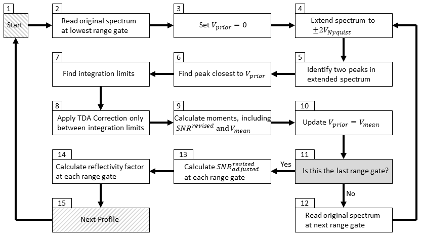
Figure A1Flow diagram to process one spectra profile as implemented in the provided Python code.
Figure A1 shows the flow diagram to process one spectra profile as implemented in the provided Python code. The processing diagram starts in box 1 in the upper left corner of Fig. A1. In box 2, the original spectrum at the lowest range gate is read into memory. The prior velocity Vprior is set to zero (box 3), which effectively assumes the spectrum velocity peak is not velocity aliased in this first range gate. The original spectrum is extended to ±2VNyquist in box 4. Box 5 identifies the two peaks in the extended spectrum. Using Vprior as the reference, the peak closest to Vprior is selected for further processing (box 6). The integration limits vstart and vend define the region containing signal power and are needed to estimate the spectrum moments (e.g. see Eq. 1). Box 7 estimates the integration limits by starting at the spectrum peak and moving down both sides of the peak until the spectrum magnitude drops below the mean noise level (Carter et al., 1995). Box 8 performs the time-domain averaging (TDA) correction, which is only applied to the signal power above between the integration limits. The spectrum moments are calculated in box 9, and the prior velocity Vprior is updated in box 10. If the current range gate is not the last range gate in the profile (box 11), then the next range gate original spectrum is read into memory (box 12), and processing continues in box 4. If the current range gate is also the last range gate in the profile (box 11), then box 13 is executed and estimates the adjusted SNR at all range gates using Eq. (5). Box 14 estimates the radar reflectivity factor at all range gates. The next profile is selected in box 15, and processing resumes in box 1.
The Python code that processes the raw Doppler velocity power spectra is available on GitHub: https://github.com/ChristopherRWilliams/RWP_Python_moments (last access: 5 April 2023, Williams, 2023a). This Python source code is also stored in an open repository with digital object identifier https://doi.org/10.5281/Zenodo.7734427 (Williams, 2023b).
All raw observations used in this study are available online using the DOE ARM data discovery tool: https://doi.org/10.5439/1025128 (ARM, 1998a), https://doi.org/10.5439/1025129 (ARM, 1998b), https://doi.org/10.5439/1025136 (ARM, 1998c), https://doi.org/10.5439/1025137 (ARM, 1998d), and https://doi.org/10.5439/1025315 (ARM, 2011). The calibrated RWP moments produced in this study are available using the DOE ARM data discovery tool: https://doi.org/10.5439/1969962 (Williams, 2023c).
CRW, PM, and SG conceptualized the study. CRW developed the spectral processing software in the MATLAB language and performed the analysis. JB converted the MATLAB code into Python code. PEJ developed the coherent integration and SNR adjustment methodologies. CRW wrote the paper, and all authors reviewed and edited the paper.
The contact author has declared that none of the authors has any competing interests.
Publisher's note: Copernicus Publications remains neutral with regard to jurisdictional claims in published maps and institutional affiliations.
This research received funding through the US Department of Energy (DOE) Atmospheric System Research (ASR) program under award DE-SC0021345. Additionally, Paul E. Johnston was supported by the NOAA Physical Sciences Laboratory and CIRES through the NOAA cooperative agreement NA17OAR4320101. We recognize and appreciate the work of field technicians deployed year-round to the Southern Great Plains and tasked with keeping these instruments running. The datasets used in this research were provided by the Office of Biological and Environmental Research of the US Department of Energy as part of the Atmospheric Radiation Measurement (ARM) Climate Research Facility.
This research has been supported by the US Department of Energy Office of Biological and Environmental Research (grant no. DE-SC0021345) and the US National Oceanic and Atmospheric Administration (NOAA) Physical Sciences Laboratory (cooperative agreement no. NA17OAR4320101).
This paper was edited by Stefan Kneifel and reviewed by three anonymous referees.
Angevine, W. M., Buhr, M. P., Holloway, J. S., Trainer, M., Parrish, D. D., MacPherson, J. I., Kok, G. L., Schillawski, R. D., and Bowlby, D. H.: Local meteorological features affecting chemical measurements at a North Atlantic coastal site, J. Geophys. Res., 101, 28935–28945, 1996.
Angevine, W. M., Grimsdell, A. W., McKeen, S. A., and Warnock, J. M.: Entrainment results from the Flatland boundary layer experiments, J. Geophys. Res., 103, 13689–13701, 1998.
ARM: Radar Wind Profiler (915RWPPRECIPMOM), 2011-03-22 to 2019-08-18, Southern Great Plains (SGP) Central Facility, Lamont, OK (C1), Compiled by Muradyan, P., Atmospheric Radiation Measurement user facility, ARM Data Center [data set], https://doi.org/10.5439/1025128, 1998a.
ARM: Radar Wind Profiler (915RWPPRECIPSPEC), 2011-03-22 to 2019-08-18, Southern Great Plains (SGP) Central Facility, Lamont, OK (C1), Compiled by Muradyan, P., Atmospheric Radiation Measurement user facility, ARM Data Center [data set], https://doi.org/10.5439/1025129, 1998b.
ARM: Radar Wind Profiler (915RWPWINDMOM), 2014-03-06 to 2019-03-10, Southern Great Plains (SGP) Central Facility, Lamont, OK (C1), Compiled by Muradyan, P., Atmospheric Radiation Measurement user facility, ARM Data Center [data set], https://doi.org/10.5439/1025136, 1998c.
ARM: Radar Wind Profiler (915RWPWINDSPEC), 2014-03-06 to 2019-03-10, Southern Great Plains (SGP) Central Facility, Lamont, OK (C1), Compiled by Muradyan, P., Atmospheric Radiation Measurement user facility, ARM Data Center [data set], https://doi.org/10.5439/1025137, 1998d.
ARM: Video Disdrometer (VDIS), 2011-03-22 to 2019-08-18, Southern Great Plains (SGP) Central Facility, Lamont, OK (C1), Compiled by Wang, D., Atmospheric Radiation Measurement user facility, ARM Data Center [data set], https://doi.org/10.5439/1025315, 2011.
ARM: Formatting and file naming protocols, Atmospheric Radiation Measurement user facility, https://www.arm.gov/guidance/datause/formatting-and-file-naming-protocols, last access: 25 April 2023.
Balanis, C. A.: Antenna Theory, John Wiley and Sons, New York, 959 pp., ISBN 0-471-59268-4, 1997.
Carter, D. A., Gage, K. S., Ecklund, W. L., Angevine, W. M., Johnston, P. E., Riddle, A. C., Wilson, J. S., and Williams, C. R.: Developments in UHF lower tropospheric wind profiling at NOAA's Aeronomy Laboratory, Radio Sci., 30, 977–1001, 1995.
Chandrasekar, V., Baldini, L., Bharadwaj, N., and Smith, P. L.: Calibration procedures for global precipitation-measurement ground-validation radars, URSI Radio Science Bulletin, 355, 45–73, 2015.
Ecklund, W. L., Carter, D. A., and Balsley, B. B.: A UHF wind profiler for the boundary layer: Brief description and initial results, J. Atmos. Ocean. Tech., 5, 432–441, https://doi.org/10.1175/1520-0426(1988)005<0432:AUWPFT>2.0.CO;2, 1988.
Farley, D. T.: On-line data processing techniques for MST radars, Radio Sci., 20, 1177–1184, 1985.
Gage, K. S. and Balsley, B. B.: Doppler radar probling of the clear atmosphere, B. Am. Meteorol. Soc., 59, 1074–1093, 1978.
Gage, K. S., Williams, C. R., and Ecklund, W. L.: UHF wind profilers: A new tool for diagnosing tropical convective cloud systems, B. Am. Meteorol. Soc., 75, 2289–2294, 1994.
Gage, K. S., Williams, C. R., Johnston, P. E., Ecklund, W. L., Cifelli, R., Tokay, A. and Carter, D. A.: Doppler radar profilers as calibration tools for scanning radars, J. Appl. Meteorol., 39, 2209–2222, 2000.
Giangrande, S. E., Wang, D., Bartholomew, M. J., Jensen, M. P., Mechem, D. B., Hardin, J. C., and Wood, R.: Midlatitude oceanic cloud and precipitation properties as sampled by the ARM Eastern North Atlantic Observatory, J. Geophys. Res.-Atmos., 124, 4741–4760, https://doi.org/10.1029/2018JD029667, 2019.
Hardin, J. and Guy, N.: PyDisdrometer (PyDSD), Zenodo [code], https://doi.org/10.5281/zenodo.9991, 2014.
Hartten, L. M., Johnston, P. E., Castro, V. M. R., and Pérez, P. S. E.: Postdeployment calibration of a tropical UHF profiling radar via surface- and satellite-based methods, J. Atmos. Ocean. Tech., 36, 1729–1751, https://doi.org/10.1175/JTECH-D-18-0020.1, 2019.
Hildebrand, P. H. and Sekhon, R. S.: Objective determination of the noise level in Doppler spectra, J. Appl. Meteorol., 13, 808–811, 1974.
Hogan, R. J., Illingworth, A. J., and Sauvageot, H.: Measuring crystal size in cirrus using 35- and 94-GHz radars, J. Atmos. Ocean. Tech., 17, 27–37, https://doi.org/10.1175/1520-0426(2000)017<0027:MCSICU>2.0.CO;2, 2000.
Kneifel, S., von Lerber, A., Tiira, J., Moisseev, D., Kollias, P., and Leinonen, J.: Observed relations between snowfall microphysics and triple-frequency radar measurements, J. Geophys. Res.-Atmos., 120, 6034–6055, https://doi.org/10.1002/2015JD023156, 2015.
Kollias, P., Puigdomènech Treserras, B., and Protat, A.: Calibration of the 2007–2017 record of Atmospheric Radiation Measurements cloud radar observations using CloudSat, Atmos. Meas. Tech., 12, 4949–4964, https://doi.org/10.5194/amt-12-4949-2019, 2019.
Mather, J. H. and Voyles, J. W.: The ARM climate research facility: A review of structure and capabilities, B. Am. Meteorol. Soc., 94, 377–392, 2013.
Merritt, D. A.: A Statistical Averaging Method for Wind Profiler Doppler Spectra, J. Atmos. Ocean. Tech., 12, 985–995, https://doi.org/10.1175/1520-0426(1995)012<0985:ASAMFW>2.0.CO;2, 1995.
Muradyan, P and Coulter, R.: Radar Wind Profiler (RWP) and Radio Acoustic Sounding System (RASS) instrument handbook, U. S. Department of Energy, Atmospheric Radiation Measurement user facility, DOE/SC-ARM-TR-044, https://doi.org/10.2172/1020560, 2020.
Myagkov, A., Kneifel, S., and Rose, T.: Evaluation of the reflectivity calibration of W-band radars based on observations in rain, Atmos. Meas. Tech., 13, 5799–5825, https://doi.org/10.5194/amt-13-5799-2020, 2020.
NOAA: Physical System Laboratory Wind Profiler Network Data and Image Library, National Oceanic and Atmospheric Administration, https://psl.noaa.gov/data/obs/datadisplay/, last access: 17 October 2022.
Palmer, R., Bodine, D., Kollias, P., Schvartzman, D., Zrnić, D., Kirstetter, P., Zhang, G., Yu, T-Y, Kumjian, M., Cheong, B., Collis, S., Frasier, S., Fulton, C., Hondl, K., Kurdzo, J., Ushio, T., Rowe, A., Salazar-Cerreño, J., Torres, S., Weber, M., and Yeary, M.: A primer on phased array radar technology for atmospheric sciences, B. Am. Meteorol. Soc., 103, E2391–E2416, https://doi.org/10.1175/BAMS-D-21-0172.1, 2022.
Protat, A., Bouniol, D., O'Connor, E. J., Baltink, H. K., Verlinde, J., and Widener, K.: CloudSat as a global radar calibrator, J. Atmos. Ocean. Tech., 28, 445–452, https://doi.org/10.1175/2010JTECHA1443.1, 2011.
Protat, A., Louf, V., Soderholm, J., Brook, J., and Ponsonby, W.: Three-way calibration checks using ground-based, ship-based, and spaceborne radars, Atmos. Meas. Tech., 15, 915–926, https://doi.org/10.5194/amt-15-915-2022, 2022.
Radenz, M., Bühl, J., Lehmann, V., Görsdorf, U., and Leinweber, R.: Combining cloud radar and radar wind profiler for a value added estimate of vertical air motion and particle terminal velocity within clouds, Atmos. Meas. Tech., 11, 5925–5940, https://doi.org/10.5194/amt-11-5925-2018, 2018.
Riddle, A. C., Hartten, L. M., Carter, D. A., Johnston, P. E., and Williams, C. R.: A minimum threshold for wind profiler signal-to-noise ratios, J. Atmos. Ocean. Tech., 29, 889–895, https://doi.org/10.1175/JTECH-D-11-00173.1, 2012.
Rogers, R. R., Ecklund, W. L., Carter, D. A., Gage, K. S., and Ethier, S. A.: Research applications of a boundary-layer wind profiler, B. Am. Meteorol. Soc., 74, 567–580, https://doi.org/10.1175/1520-0477(1993)074<0567:RAOABL>2.0.CO;2, 1993.
Schmidt, G., Rüster, R., Czechowsky, P.: Complementary codes and digital filtering for detection of weak VHF radar signals from the mesosphere, IEEE T. Geosci. Elect., GE-17, 154–161, 1979.
Schönhuber, M., Lammer, G., and Randeu, W. L.: The 2D-Video-Disdrometer, in: Precipitation: Advances in Measurement, Estimation and Prediction, Springer, Heidelberg, Germany, 3–31, https://doi.org/10.1007/978-3-540-77655-0_1, 2008.
Tapiador, F. J., Navarro, A., Moreno, R., Jiménez-Alcázar, A., Marcos, C., Tokay, A., Durán, L, Bodoque, J. M., Martín, R., Petersen, W., and de Castro, M.: On the optimal measuring area for pointwise rainfall estimations: A dedicated experiment with 14 laser disdrometers, J. Hydrometeorol., 18, 753–760, https://doi.org/10.1175/JHM-D-16-0127.1, 2017.
Tokay, A., Kruger, A., and Krajewski, W. F.: Comparison of drop size distribution measurements by impact and optical disdrometers, J. Appl. Meteorol. Clim., 40, 2083–2097, https://doi.org/10.1175/1520-0450(2001)040<2083:CODSDM>2.0.CO;2, 2001.
Tokay, A., Petersen, W. A., Gatlin, P., and Wingo, M.: Comparison of raindrop size distribution measurements by collocated disdrometers, J. Atmos. Ocean. Tech., 30, 1672–1690, https://doi.org/10.1175/JTECH-D-12-00163.1, 2013.
Tridon, F., Battaglia, A., Kollias, P., Luke, E., and Williams, C. R.: Signal postprocessing and reflectivity calibration of the Atmospheric Radiation Measurement Program 915-MHz Wind Profilers, J. Atmos. Ocean. Tech., 30, 1038–1054, https://doi.org/10.1175/JTECH-D-12-00146.1, 2013.
Wang D., Bartholomew, M., Giangrande, S. E., and Hardin, J. C.: Analysis of three types of collocated disdrometer measurements at the ARM southern great plains observatory, U. S. Department of Energy, Atmospheric Radiation Measurement user facility, DOE/SC-ARM-TR-275, https://doi.org/10.2172/1828172, 2021.
Wilfong, T. L., Merritt, D. A., Lataitis, R. J., Weber, B. L., Wuertz, D. B. and Strauch, R. G.: Optimal generation of radar wind profiler spectra. J. Atmos. Ocean. Tech., 16, 723–733, 1999.
Williams, C. R.: Vertical air motion retrieved from dual-frequency profiler observations, J. Atmos. Ocean. Tech., 29, 1471–1480, https://doi.org/10.1175/JTECH-D-11-00176.1, 2012.
Williams, C. R.: How much attenuation extinguishes mm-wave vertically pointing radar return signals?, Remote Sens., 14, 1305, https://doi.org/10.3390/rs14061305, 2022.
Williams, C. R.: Radar Wind Profiler (RWP) processing codes in Python, GitHub [code], https://github.com/ChristopherRWilliams/RWP_Python_moments (last access: 5 April 2023), 2023a.
Williams, C. R.: Radar Wind Profiler (RWP): Calculate spectrum moments using Python code, Zenodo [code], https://doi.org/10.5281/zenodo.7734427, 2023b.
Williams, C. R.: Calibrated Radar Wind Profiler (RWP) moments from SGP, Atmospheric Radiation Measurement user facility, ARM Data Center [data set], https://doi.org/10.5439/1969962, 2023.
Williams, C. R., Gage, K. S., Clark, W., and Kucera, P.: Monitoring the reflectivity calibration of a scanning radar using a profiling radar and a disdrometer, J. Atmos. Ocean. Tech., 22, 1004–1018, 2005.
Williams, C. R., Maahn, M., Hardin, J. C., and de Boer, G.: Clutter mitigation, multiple peaks, and high-order spectral moments in 35 GHz vertically pointing radar velocity spectra, Atmos. Meas. Tech., 11, 4963–4980, https://doi.org/10.5194/amt-11-4963-2018, 2018.