the Creative Commons Attribution 4.0 License.
the Creative Commons Attribution 4.0 License.
 | 30 May 2023
Using a deep neural network to detect methane point sources and quantify emissions from PRISMA hyperspectral satellite images
Peter Joyce
Cristina Ruiz Villena
Yahui Huang
Alex Webb
Manuel Gloor
Fabien H. Wagner
Martyn P. Chipperfield
Rocío Barrio Guilló
Chris Wilson
Anthropogenic emissions of methane (CH4) have made a considerable contribution towards the Earth's changing radiative budget since pre-industrial times. This is because large amounts of methane are emitted from human activities, and the global warming potential of methane is high. The majority of anthropogenic fossil methane emissions to the atmosphere originate from a large number of small (point) sources. Thus, detection and accurate, rapid quantification of such emissions are vital to enable the reduction of emissions to help mitigate future climate change. There exist a number of instruments on satellites that measure radiation at methane-absorbing wavelengths, which have sufficiently high spatial resolution that can be used for detecting plumes of highly spatially localised methane “point sources” (areas on the order of m2 to km2). Searching for methane plumes in methane-sensitive satellite images using classical methods, such as thresholding and clustering, can be useful but is time-consuming and often involves empirical decisions. Here, we develop a deep neural network to identify and quantify methane point source emissions from hyperspectral imagery from the PRecursore IperSpettrale della Missione Applicativa (PRISMA) satellite with 30 m spatial resolution. The moderately high spectral and spatial resolution, as well as considerable global coverage and free access to data, makes PRISMA a good candidate for methane plume detection. The neural network was trained with simulated synthetic methane plumes generated with the large eddy simulation extension of the Weather Research and Forecasting model (WRF-LES), which we embedded into PRISMA images. The deep neural network was successful at locating plumes with a F1 score, precision, and recall of 0.95, 0.96, and 0.92, respectively, and was able to quantify emission rates with a mean error of 24 %. The neural network was furthermore able to locate several plumes in real-world images. We have thus demonstrated that our method can be effective in locating and quantifying methane point source emissions in near-real time from 30 m resolution satellite data, which can aid us in mitigating future climate change.
- Article
(4370 KB) - Full-text XML
-
Supplement
(1281 KB) - BibTeX
- EndNote


Methane (CH4) is a powerful greenhouse gas with a warming potential which, per unit mass emitted, is 84 times larger than for carbon dioxide over a 20-year period (Stocker et al., 2013). Emissions of methane as a result of human activities have contributed to one-quarter of climate warming since pre-industrial times (Etminan et al., 2016). A large proportion of anthropogenic methane from industrial sources originates from point sources such as coal mines and oil and gas production facilities (Saunois et al., 2020). Furthermore, these emissions are generally underestimated by inventory-based approaches (Alvarez et al., 2018; Karion et al., 2013; Zavala-Araiza et al., 2015). A large proportion of these anthropogenic emissions originates from a small number of strong point sources due to oil and gas production equipment malfunction (Brandt et al., 2016; Duren et al., 2019; Zavala-Araiza et al., 2017). Consequently, much of the methane emitted from such sources could be reduced at no net cost (IEA, 2017; Ocko et al., 2021). Acting to reduce methane emissions in this sector could be one of the most cost-effective methods of mitigation against further climate change.
Methane point sources from oil and gas production are typically small in extent, and emissions are difficult to quantify and variable in time (Allen et al., 2013; Frankenberg et al., 2016; Cusworth et al., 2021b). The primary challenge faced when estimating methane emissions from point sources from satellite data comes from the relatively low spatial resolution (in the order of kilometres) of satellite imagery from dedicated sensors such as the Greenhouse Gases Observing SATellite (GOSAT) (Kuze et al., 2009) and the TROPOspheric Monitoring Instrument (TROPOMI) (Levelt et al., 2006). These sensors typically have high spectral resolution of methane absorption bands in the shortwave infrared (SWIR) range of the electromagnetic spectrum to provide accurate measurements with high precisions of around 10–20 ppb (parts per billion) (Lorente et al., 2021; Parker et al., 2020). SWIR bands can also be effectively utilised to detect and quantify point sources from lower-spectral-resolution sensors (Jacob et al., 2016; Duren et al., 2019). Recent hyperspectral spaceborne imaging spectrometers contain hundreds of spectral channels in the visible–shortwave infrared range, with spectral resolution typically around 10 nm and spatial resolutions of tens of metres. Due to their spatial and spectral resolution, they have been identified as useful new tools for identifying and quantifying methane point source emissions. PRecursore IperSpettrale della Missione Applicativa (PRISMA), developed and operated by the Italian Space Agency (ISA) since 2019, is the first hyperspectral mission where the satellite imagery has been openly released to the scientific community. The satellite consists of a panchromatic camera and an advanced hyperspectral instrument that measures radiances in approximately 250 bands between 400 and 2500 nm. The instrument has a spatial resolution of 30 m, a swath of 30 km, and a 12 nm spectral resolution (Galeazzi et al., 2008). PRISMA has been successful in quantifying CO2 emissions from coal- and gas-fired power plants (Cusworth et al., 2021a). However, how to best extract information on the location and extent of methane plumes is not yet fully established. Successful detection of methane point sources from PRISMA using a matched-filter retrieval technique has been reported by Guanter et al. (2021), albeit with a strong dependence of detection accuracy on surface type. In particular, brightness and homogeneity of the satellite images were identified to significantly influence the accuracy of methane detection techniques.
Current approaches for detecting methane point sources and quantifying emission rates are time-intensive and laborious and can be prone to errors without sufficient training. They typically involve a spectral analysis of satellite data to infer methane column mean mixing ratios (Thorpe et al., 2014) followed by a methane plume detection method (often based on thresholding and clustering) and finally the integrated mass enhancement (IME) method to estimate the emission (Varon et al., 2018). Previous efforts utilising spaceborne imaging spectrometers to quantify methane point source emission rates have proved successful but often with large errors of source detection and emissions estimates. The IME method yielded errors between 5 % and 12 % using 50 m resolution Greenhouse Gas Satellite – Demonstrator (GHGSat-D) imagery (Varon et al., 2018). However, this uncertainty estimate does not include errors from unknown wind speed and direction, which are both highly uncertain, where uncertainties are estimated to be 15 %–65 % larger. The multi-band multi-pass (MBMP) method was successful in quantifying methane point source emissions from Sentinel-2 multispectral instrument (MSI) imagery, with precision between 30 % and 90 % (Varon et al., 2021). The primary limitation of this approach is surface interference (Cusworth et al., 2019) which leads to artefacts and false anomalies, which can be mistakenly attributed to emission plumes. This is a major disadvantage for multi- and hyperspectral missions because the better the resolution (and the greater the number of channels), the better the discrimination between the surface and methane absorption. Sherwin et al. (2023) found comparatively lower errors but required considerable human intervention. Thus, producing a model that minimises errors and can automatically locate methane sources would make emission monitoring from space faster, more reliable, and more scalable, thus providing an invaluable tool to aid mitigation. A first effort has also been made to estimate emission rates from AVIRIS-NG data using a neural network and without utilising wind speed and direction data. These estimates were subject to an error of roughly 30 % of the emission rates (Jongaramrungruang et al., 2019). It is apparent that the noise in the satellite data, the lack of accurate wind data, and the complex structures of methane plumes make it difficult to model emission rates accurately via traditional approaches.
In recent years, deep neural network methods have improved rapidly. LeNet (LeCun et al., 1989) was one of the earliest convolutional neural networks (CNNs) and was used successfully to identify handwritten digits. This work laid the foundations for using artificial intelligence to obtain meaningful information from image data (known as computer vision). Deep learning models entered the mainstream following considerable reductions in model training time through the utilisation of graphics processing units (GPUs) (Oh and Jung, 2004). Deep learning was then revolutionised for image classification with the introduction of AlexNet (Krizhevsky et al., 2017). CNNs have since been applied to self-driving cars (e.g. Nugraha and Su, 2017), the discovery of new drug treatments (e.g. Wallach et al., 2015), facial recognition (e.g. Matsugu et al., 2003), and many other applications. The ease with which deep neural networks can be trained and deployed has also improved considerably in recent years, partially due to the development of application programming interfaces (APIs), such as Keras (Chollet, 2015). This has been supplemented by the increasing ubiquity and decreasing costs of GPUs and cloud computing servers, which together have enabled deep learning models to be trained rapidly and at a relatively low cost. Currently, work utilising deep neural networks has already proven to be considerably more effective than classical methods to detect point source emissions of nitrogen dioxide (NO2) (Finch et al., 2022).
More recently, a deep neural network has been used to quantify methane point source emissions using the airborne AVIRIS-NG instrument (Jongaramrungruang et al., 2022). In this study, a CNN was trained on synthetic plumes inserted into real images to extract features present in plumes of varying intensities and with differing wind speeds to locate and quantify the emission rates of the point sources. Jongaramrungruang et al. (2022) estimated emission rates of plumes with a mean absolute error of 17 % for emissions larger than 40 kg h−1. The classification accuracy (determining whether a plume is present in an image) was 90 % when testing plumes with emission rates above 100 kg h−1; however, the accuracy dropped to 50 % for emission rates around 50–60 kg h−1. The spatial and spectral resolution of the aircraft data used in this study (AVIRIS-NG) has far higher spatial and spectral resolution than PRISMA, thus making methane detection prone to lower errors. However, PRISMA data are publicly available and cover a far larger spatial range with regular repeat measurements, thus making it a superior resource for rapid detection of methane point source emissions across many regions on earth. Thus, a deep neural network that is capable of utilising PRISMA data to detect methane emissions could be very effective in our efforts to mitigate future climate change.
In this study, we produced pseudo-observations of simulated synthetic methane plumes generated with the large eddy simulation extension of the Weather Research and Forecasting model (WRF-LES). These simulated plumes were then embedded into an array of PRISMA images and used as training data for a novel neural network architecture that aimed to produce masks of the locations of methane plumes and estimate their emission rates from PRISMA satellite imagery. The effectiveness of this model was then tested on images of real-world plumes. The results from the neural network were then compared with a classical technique that combined PCA-based retrievals with clustering using DBSCAN. The techniques utilised here can be adapted to locate and quantify emission rates using any satellite imagery with suitable shortwave-infrared bands or applied to detecting other greenhouse gases, such as carbon dioxide (CO2).
2.1 Simulating methane plumes with WRF-LES
The Weather Research and Forecasting (WRF) model system has comprehensive and multiple capabilities for studying atmospheric phenomena from global down to large eddy scales. The default large eddy simulation case (LES) of the WRF V4.2.2 was used and modified to simulate methane plumes for a single point source with a release rate of 1000 kg h−1. The default LES case does not consider clouds, radiation, or topography but includes surface physics and 1.5-order TKE (turbulent kinetic energy) prediction scheme (WRF model User's Guide: https://www2.mmm.ucar.edu/wrf/users/, last access: 15 March 2022). A constant thermal flux of 100 W m−2 was applied at the surface to drive the turbulence. Two nested domains with one-way nesting were deployed in the simulations. The outer domain had a size of 5.4 km × 6.3 km, with 90 m horizontal resolution and periodic boundary conditions. The inner domain had a size of 3.6 km × 4.5 km, with 30 m horizontal grid spacing and 30 m vertical resolution and flow-dependent boundary conditions for scalars. The plume was only released in the inner domain after a 3 h spin-up run. The total running time is 5 h, and the final 2 h run was considered for the training, test, and validation data.
We designed 15 scenarios consisting of five different southerly wind speeds ranging from 1 to 9 m s−1, each of which was uniformly applied from the surface to the model top, and three different patterns of potential temperature vertical profiles (Fig. S1 in the Supplement). The potential temperature in the scenarios is specified as 290 K from the surface to one of the 3 different mixing depths of 500, 800, and 1100 m (Fig. S2). Above the mixing depth, there is an inversion layer of 700 m with a vertical gradient of potential temperature of 0.009 K m−1 applied from the top of the mixing layer to the model top. For each simulation, the CH4 distribution is saved once every minute, and thus there are 120 different scenes for a 2 h simulation. Altogether there are 1800 scenes for the 15 simulations in the data, where the plume was integrated over vertical columns. Figure 1 shows one snapshot of a plume with initial conditions of 3 m s−1 southerly wind and 800 m mixing depth 30 min after release.
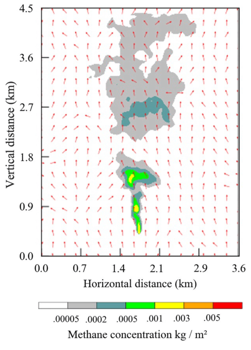
Figure 1Snapshot of a simulated plume 30 min after release for initial conditions of 3 m s−1 southerly wind and 800 m mixing depths. Red arrows indicate wind direction at the moment of the snapshot.
2.2 Satellite data retrieval
Methane absorbs solar radiation at a set of shortwave-infrared wavelengths that are well known and documented in spectroscopic databases. The absorption of light by methane in the atmosphere therefore alters the reflected sunlight measured by the satellite in a very predictable way that allows us to quantify the amount of methane along the light path. Here we use a data-driven retrieval algorithm to estimate the methane enhancements from reflected sunlight using statistical methods based on the work by Thorpe et al. (2014). This type of simple and fast retrieval method is commonly used for instruments with comparably low spectral resolutions, for which a more sophisticated, so-called full-physics approach provides no extra benefit.
The relationship between the spectral intensity at each point in the satellite spectra and the column enhancement of methane in the scene is represented by a methane Jacobian vector, which describes the change in the logarithm of the intensity Ik in band k with respect to the column enhancement of methane . The spectral variation of the background of the scene (i.e. outside of the plume) is approximated by a number of principal components of all measured spectra combined derived using the principal component analysis (PCA) method. We perform the PCA on the logarithm of measured spectra of the scene and select the singular vectors (principal components) that best describe the spectral variability of the scene. The optimal number of singular vectors was determined by trial and error, and was found to be the first three. We then concatenate these vectors with the methane Jacobian to construct the matrix J with dimension 4× number of PRISMA bands, which we use along with the logarithm of the measured radiances, y, to find a vector W that minimises the cost function in a linear least squares fit for each pixel:
The modelled radiance F is calculated from J and W as follows:
We can then rewrite Eq. (2) as the sum of the background (k) and CH4 (c+1) components of the radiance:
where c is the number of singular vectors used. Thus, the modelled logarithmic radiance F(W,J) is a linear combination of the singular vectors, Jk, the CH4 Jacobian, Jc+1, and their weights, Wk and Wc+1, respectively. This method is described in more detail in Thorpe et al. (2014). In order to avoid column-wise changes in the instrument's radiometric response, and since the wavelengths scale for each across-track pixel of a PRISMA image is different, it is necessary to infer the principal components for each column in the across-track direction separately.
2.3 Training data generation
We generated synthetic datasets to train the machine-learning model by combining PRISMA images with the synthetic plumes simulated with WRF-LES (described in Sect. 2.1). We use the SWIR spectral radiance from PRISMA Level-1b data as well as the RGB bands. These datasets come with pixel quality and cloud mask information, which we apply in our data preparation process. We selected 36 different PRISMA background images to cover a wide range of scenes representative of places where methane plumes might be expected (Table S1 in the Supplement). These images also cover a range of different dates throughout the ∼3 years of PRISMA data available in the archive, to account for different illumination conditions. All the selected scenes have less than 1 % cloud cover, and any pixels flagged as cloudy in the PRISMA product were excluded from the analysis.
A total of 9700 image tiles were generated for training, each tile with a size of 256×256 pixels. The tile size was deliberately selected as a power of 2 to optimise the model performance. Each tile was selected at random from one of the 36 1000×1000-pixel PRISMA background scenes, and a synthetic methane plume was subsequently embedded in it. The synthetic plume was also selected randomly from the WRF-LES simulations, with the following parameters also randomised following a uniform distribution:
-
Time step. A time step of between 1 and 120 s is used (Fig. S3).
-
Plume origin. This includes any point within the background scene tile, excluding the areas near the edges to avoid missing parts of the plume.
-
Emission rate. All simulated plumes have a 1000 kg h−1 emission rate, so we applied a scaling factor between 0.1 and 10 to have a range between 100 and 10 000 kg h−1 (Fig. S4).
The synthetic plumes from WRF-LES are first converted into maps of methane vertical column densities (in molecules cm−2). The original plume simulations are all carried out for an emission of 1000 kg h−1, and the scenarios for different emission rates are obtained by scaling the simulated concentrations. Each plume is inserted into the background PRISMA image tile by modifying the PRISMA SWIR radiances according to the Beer–Lambert law for absorption. Methane columns are converted into optical depth for each band using a representative methane absorption cross-section for each band computed from the HITRAN database (Gordon et al., 2022) for a temperature of 293 K and pressure of 1 atmosphere. The use of a single temperature and pressure value is a simplification that could introduce small uncertainties for vertically extended plumes. Each of the 9700 training datasets contains 38 PRISMA radiance bands (3 RGB and 35 SWIR (2100–2365 nm) channels) and the synthetic plume (i.e. the “true” methane enhancements to be used as labels in the model).
2.4 Training data processing
Each PRISMA sub-image (256×256-pixel tile) was normalised by subtracting the mean and dividing it by the standard deviation (SD) of the whole collection of training images such that the mean of all the images was 0 and the SD was 1 for each band. This data normalisation step is standard when using deep neural networks as it is understood to optimise the training time. Following on from this, the undefined (NaN, not a number) values present in the images were changed to equal the mean value of each band in the respective image. These NaN values correspond to either invalid (e.g. saturated) or cloudy pixels.
Every time an image was retrieved during the training process, data augmentations were randomly applied. The augmentations were as follows: rotation by a multiple of 90∘ and horizontal and vertical flipping. No brightness and contrast augmentations were made because the quantification of methane plumes relies on the specific band information inside the plume region. The purpose of data augmentation was to increase the data volume, to reduce overfitting, and to improve the ability of the model to produce accurate results with data that is different to the training data.
To predict the methane concentration, it was first necessary to model the methane plume mask (binary classification of plume/non-plume per pixel) because the vast majority of pixels in the training images did not contain a plume (zero-inflated data). To create the ground truth masks for binary segmentation, an initial methane concentration threshold of 8×10¹⁸ molecules cm−2 was chosen as it was the cut-off point where the plumes were no longer visible. Furthermore, training the model with a lower threshold resulted in non-convergence. After the model was trained at the 8×10¹⁸ molecules cm−2 threshold, it was possible to continue training the model at a lower threshold. Thus, we tested training the model at 5×10¹⁷ molecules cm−2 increments until the validation loss dropped substantially. The lowest threshold where this was the case was 4×10¹⁸ molecules cm−2. This final step is important because it increases the range for which the model can locate and quantify methane emissions.
2.5 Deep neural network architecture and training process
The training of the neural network was split into four steps. First, the model was trained to locate the regions of the image containing a plume via per pixel binary semantic segmentation. Next, the column enhancements of methane were predicted inside the region of the estimated plume mask from the first stage. Following on from this, the emission rate of the plume in the image was estimated. To ensure that the emission rate estimates would equal zero when no plume was present, an intermediate prediction layer was included where a whole image binary classification was made regarding whether a plume was present in the image or not. At each stage of the model, the input was a concatenation of the input satellite image and all the previous outputs (Fig. 2). To optimise the training of the model weights, each portion of the model was trained alone such that the weights in all the other parts were not being updated. The parts of the model were trained in order, moving downwards across the models depicted in Fig. 2. The loss function to predict the plume mask was as follows:
where BC is binary cross-entropy, and SDC is the Sørensen–Dice coefficient, defined as follows:
where TP is true positive, FN is false negative, and FP is false positive. This loss function was chosen because of the large number of non-plume pixels present in the image. The loss function for the mask concentration was mean squared error (MSE), a standard choice for regression modelling. For the whole image binary classification part of the model, binary cross-entropy was chosen, which is common for solving 1-dimensional binary problems. Finally, for the emission rate part of the model, MSE was chosen as the loss function until the validation error started to plateau, after which the model was only trained on images containing plumes, and mean absolute percentage error was given as the loss function. This was done to ensure that the proportion error was minimised rather than the absolute error. Mean absolute percentage error was not used throughout the whole training process because it was important that the model was trained on some images with no plumes (so an emission rate of zero could be possible), and mean absolute percentage error produced very high loss values when false positives were made by the model.
For plume mask detection, a UNet model was used, and for methane concentration, a ResNet model was used. For the whole image binary plume detection and emission rate estimation, however, CNNs with only an encoder branch were used. The two encoder CNNs have identical architectures except that the activation function at the end of the whole image binary classification model has sigmoid activation because the predictions are constrained between 0 and 1, and the emission rate estimator has a ReLU activation function.
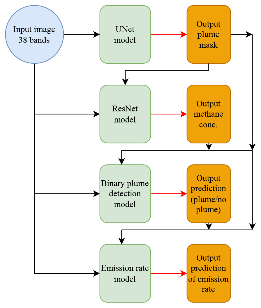
Figure 2Structure of the neural networks used in this study. Green boxes indicate portions of the neural network, and orange boxes indicate predictions made by each stage of the neural network. Black lines indicate flow of data into models, and red lines indicate predictions resulting from a model.
2.5.1 Estimating plume masks
Estimating the mask of a methane plume involved using a similar architecture to a UNet model (Ronneberger et al., 2015) (Fig. 3). UNet models consist of two paths; the first is the encoder, which captures the context in the image and is composed of convolutional and max pooling layers. The second path is the decoder, which enables localisation of the features captured by the encoder and consists of convolutional and upsampling layers (Ronneberger et al., 2015). In our model architecture, there is an additional 1×1 convolutional layer with 64 filters at the beginning because methane plumes are associated with anomalies in certain SWIR bands of the PRISMA imagery. This additional convolution makes the network pay closer attention to individual pixel values in the satellite data rather than focussing more on the shapes present in the image. Methane does not absorb in the visible bands; thus, the inclusion of the visible bands helps the neural network to distinguish between plume and non-plume by providing information on the background of the image. Methane plumes can be identified based on the typical spatial structures that form as a result of turbulence and advection in the atmosphere, as well as the variations in methane-absorbing bands compared with the background landscape. It is the latter reason why an additional 1×1 convolutional layer was deemed to be helpful in improving the accuracy of the model.
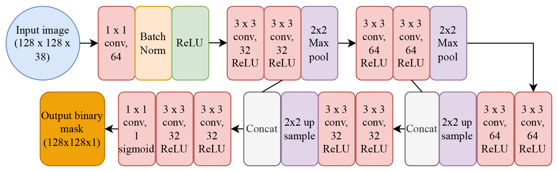
Figure 3Architecture of the deep neural network for the UNet portion of the model. “1×1 conv, 64” refers to a convolutional filter with kernel size 1×1 and 64 filters. “Batch Norm” refers to a batch normalisation layer, “Concat” refers to a concatenation between the inputs to that layer, “2×2 Max pool” refers to a max pooling layer with pool size 2, and “2×2 up sample” refers to upsampling layer with size 2. “ReLU” and “sigmoid” refer to the rectified linear unit and sigmoid activation functions respectively.
2.5.2 Estimating methane column enhancements inside plumes
Estimating the methane column enhancement within the plumes predicted in Sect. 2.4.1 uses a concatenation of the input image and the mask predictions. This step to aid the estimation of methane concentrations is necessary because the vast majority of pixels do not contain a plume (a zero-inflated regression problem). Such problems often have the issue that the model will converge at predicting zeros everywhere. Thus, the inclusion of the mask prediction helps to prevent this. The ensuing model is composed initially of a 1×1 convolutional layer for a similar reason as its inclusion in the UNet model (see Sect. 2.5.1). Following on from this are two ResNet layers (He et al., 2016), which are characterised by double-layer skip connections, ReLU activation functions, and batch normalisation (Fig. 4). A ResNet architecture was selected for this portion of the model as it is known to be lightweight and powerful at regression predictions in computer vision.
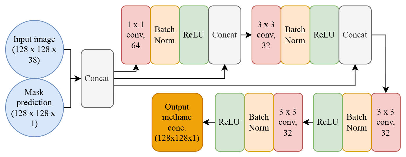
Figure 4Architecture of the deep neural network for the ResNet portion of the model. “1×1 conv, 64” refers to a convolutional filter with kernel size 1×1 and 64 filters. “Batch Norm” refers to a batch normalisation layer, and “Concat” refers to a concatenation between the inputs to that layer. “ReLU” refers to the rectified linear unit activation function.
2.5.3 Estimating emission rate of plumes
The prediction of the whole image binary classification of plume/not plume involved an architecture identical to the one presented in this section (except that the final activation layer was sigmoid, not ReLU). The inputs to the emission rate portion of the model are the outputs from all the previous stages of the model concatenated with the input image. The outputs of the mask prediction and whole image binary segmentation are continuous between 0 and 1. The majority of the methane concentration output is also in this range because the methane concentration ground truth was preprocessed via min–max normalisation (to optimise training time). This is to ensure that more information is available to the model to accurately estimate emission rates. Following on from this is the 1×1 convolutional layer, which was included for the same reason as in the previous stages of the model (see Sect. 2.5.1). This is followed by the encoder part of the model, in which a convolutional layer is followed by batch normalisation, ReLU activation, and max pooling, which is done seven times with increasing filters every second loop. These layers encode features about the methane plumes and reduce the dimensionality of the tensors. Finally, there is a dense layer and ReLU activation to collect all information obtained and output a single floating-point number as the predicted emission rate (Fig. 5).
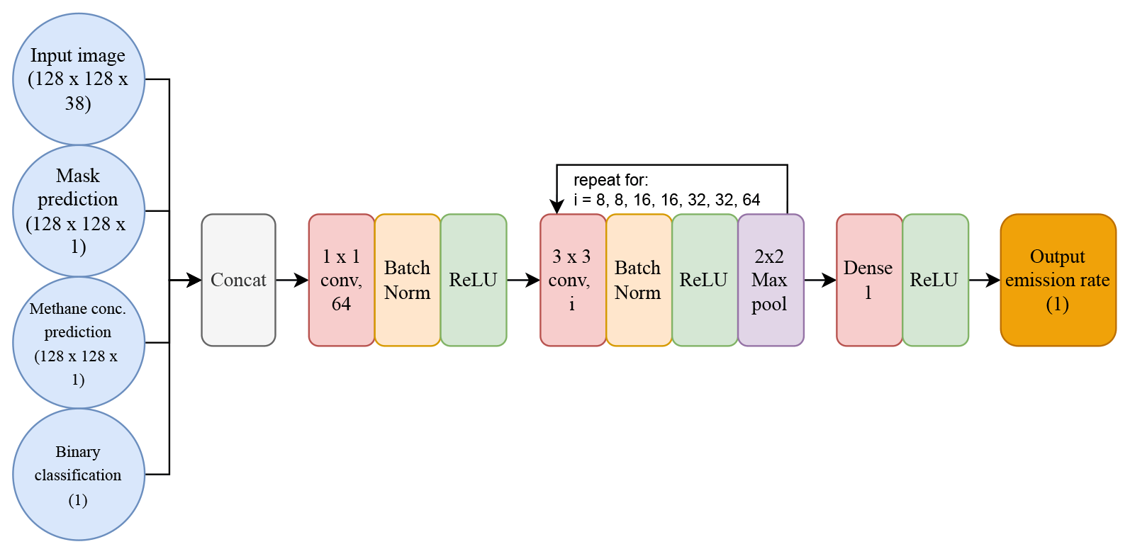
Figure 5Architecture of the deep neural network for the emission rate prediction of the model. “1×1 conv, 64” refers to a convolutional filter with kernel size 1×1 and 64 filters. “Batch Norm” refers to a batch normalisation layer, “Concat” refers to a concatenation between the inputs to that layer, and “2×2 Max pool” refers to a max pooling layer with pool size 2. “ReLU” refers to the rectified linear unit activation function.
3.1 Application of neural network to simulated plumes
The total training–validation dataset consisted of 9700 images, 80 % of which were reserved for training and the remaining 20 % for validation. After each iteration of the model through the training dataset (known as an epoch), the model was tested on the validation dataset. If the loss of the model when tested on the validation dataset was lower than the lowest loss previously recorded, the weights of the model were updated. Thus, at the end of the training procedure, the best model was saved. Each of the stages of the model depicted in Fig. 2 were trained separately in descending order, where the weights of the other stages did not vary. This was done so that the most accurate predictions were being produced from the earlier layers so that no errors from insufficient training would propagate through the model because the outputs are concatenated with the satellite data in later parts of the model.
Once training was complete, the model was tested on an additional 2000 images not seen during training sampled randomly from a uniform distribution of emission rates from 500 to 10 000 kg h−1. Out of the 2000 images, 36 had a maximum methane concentration under the 4×10¹⁸ molecules cm−2 threshold imposed during training; however they were still included in the testing to determine if they could still be detected by the model. The model is able to accurately locate and identify the shape of methane plumes in the test dataset (Fig. 6).
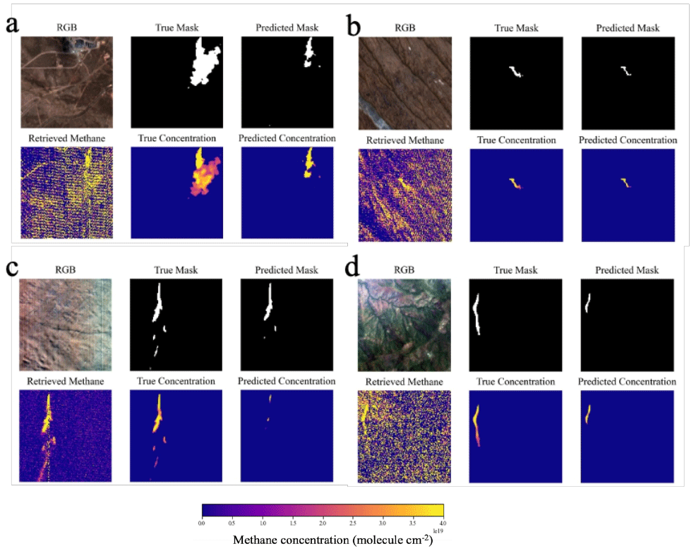
Figure 6Example images and predictions taken from the test dataset. Images are 3840×3840 m composed of 128×128-pixel tiles. True emission rates and initial wind speeds are (a) 8068 kg h−1 and 1 m s−1, (b) 1484 kg h−1 and 1 m s−1, (c) 7673 kg h−1 and 5 m s−1, and (d) 6270 kg h−1 and 4 m s−1. Retrieved methane comes from the retrieval described in Sect. 2.2. RGB image courtesy of PRISMA (© Italian Space Agency).
The average methane column enhancement in the images was well estimated, where average estimated methane was closely correlated with the ground truth (Fig. 7) with a tendency to slightly overestimate column values. This is possibly because predicted methane masks were generally smaller than the true masks, so during training, the methane concentration model overpredicted the centre of the plumes to compensate for this.
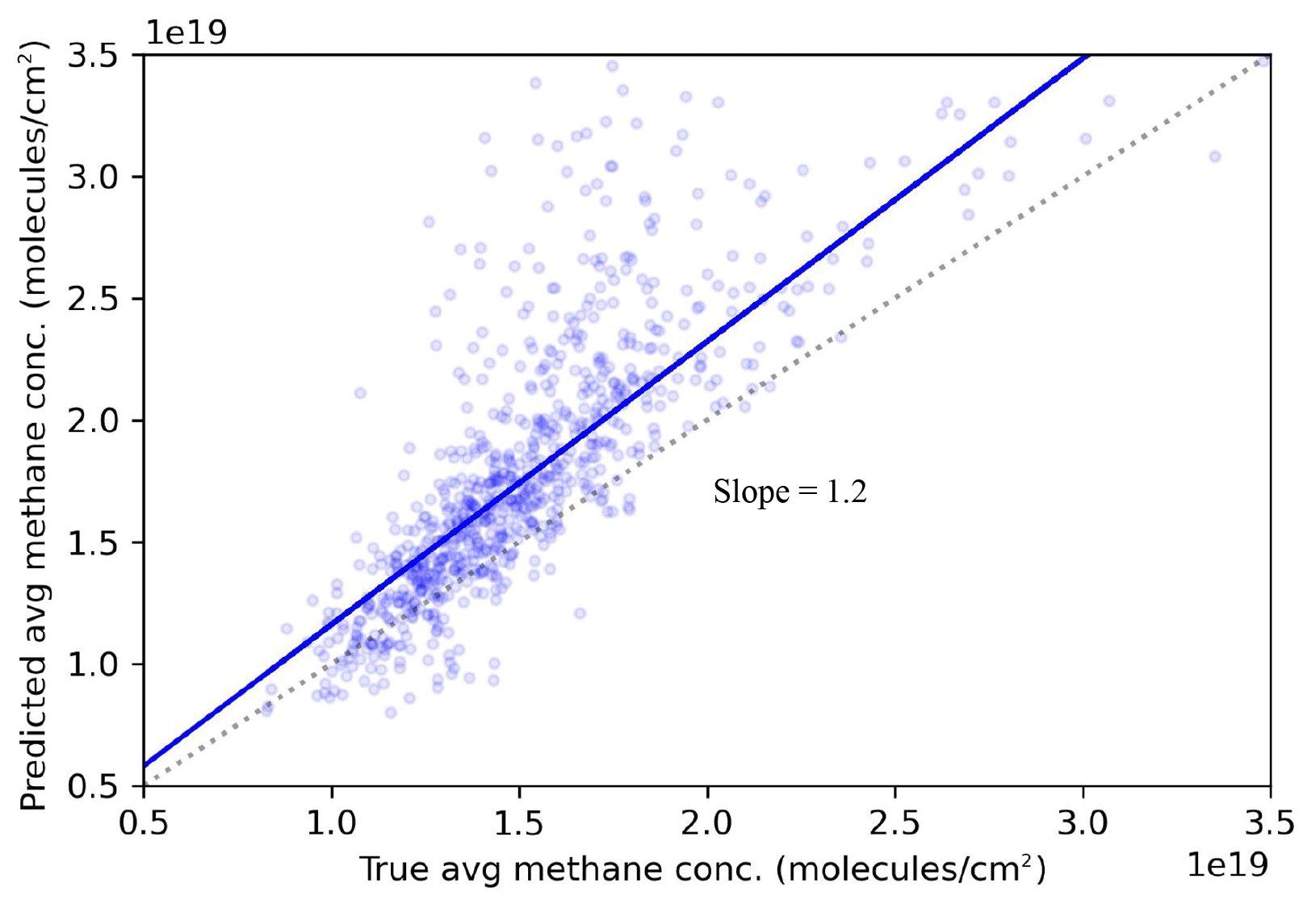
Figure 7Scatter plot of predicted vs. true mean methane concentration. The true (predicted) average methane concentration was calculated from the average inside the true (predicted) plume.
In the whole image binary classification part of the model, we assess its success using the F1 score, precision, and recall, which are defined as follows:
In the whole image binary classification part of the model, the F1 score, precision, and recall were 0.95, 0.96, and 0.92, respectively (Table 1). These statistics come from predictions made on the 2000 images with plumes in, as well as an additional 1533 images with no plumes.
Table 1Confusion matrix of whole image binary classification portion of the model broken down per image.
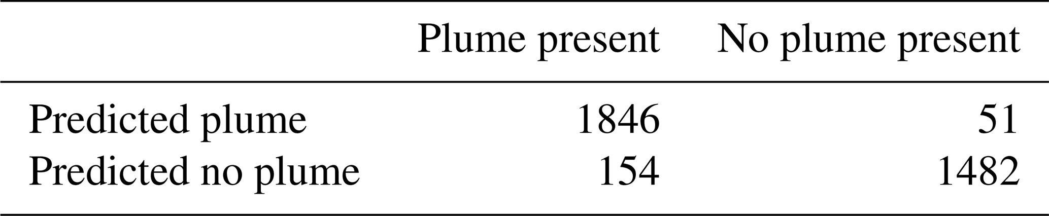
The distributions of the scene noise and methane concentrations in the cases where no plume was predicted but a plume was present (false negative) reveal scene noise that is slightly lower than average and maximum methane concentration that is much lower than average (Table S2). However, in the cases where a plume was predicted but no plume was present (false positive), scene noise is not noticeably different (Table S2).
The actual vs predicted emission rate has a slope of 0.83, with a relatively small spread about the line of best fit (SD =1447 kg h−1). This means that there is a tendency for underestimating emissions with a mean absolute percentage error in emission rate of 23.7 % (Fig. 8). Underpredictions are common in regression models, especially when data points with zeros are included such as in this case because the model was trained on images without plumes as well as those containing plumes. This was a necessary step, however, because the model did not converge so well without these images, and predictions were far worse at lower emission rate ranges.
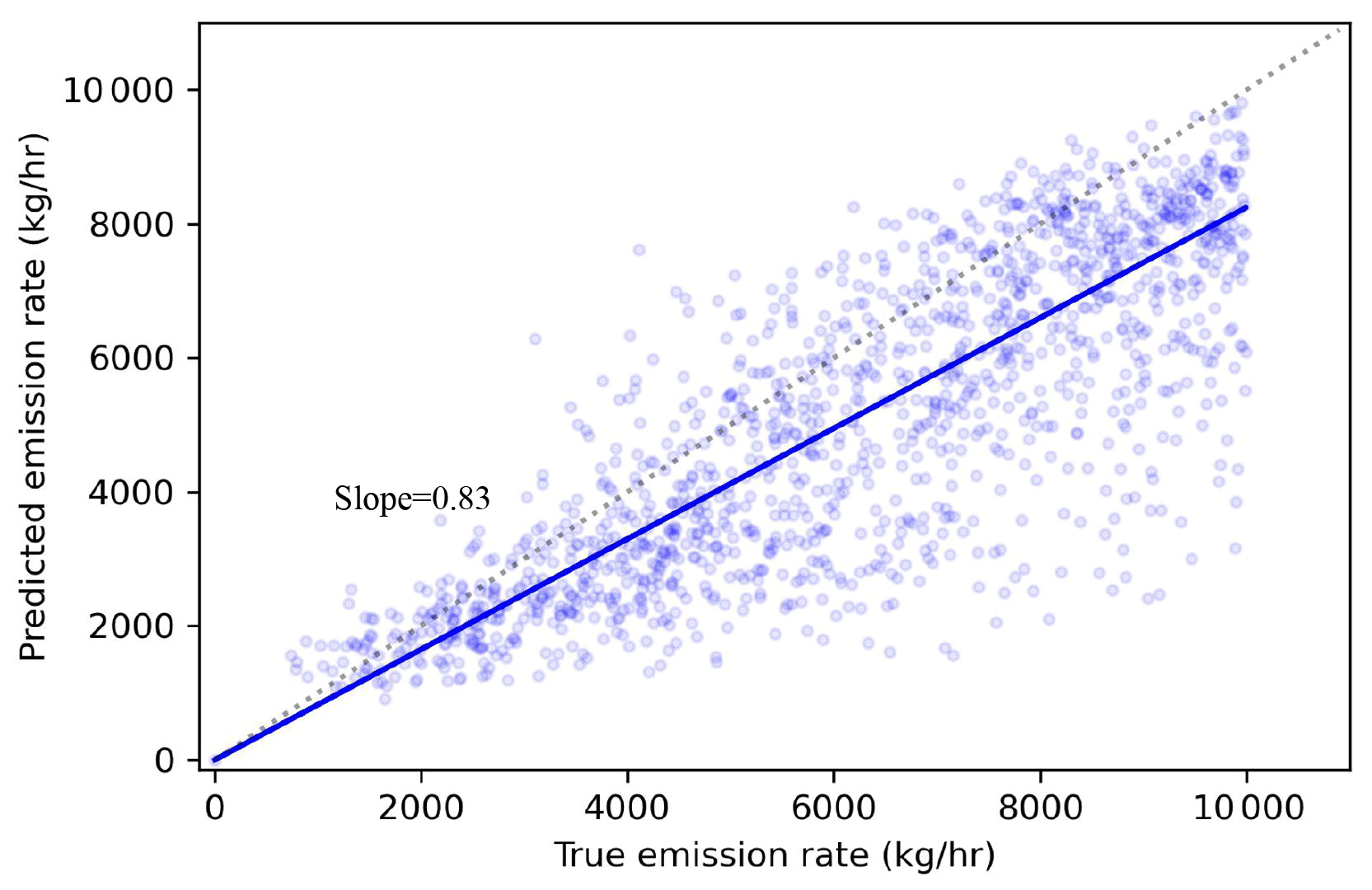
Figure 8Actual vs. predicted emission rate using the deep learning model. Line of best fit calculated using Huber loss, so outliers do not have an inordinate influence on the slope.
The absolute emission rate error increased in magnitude as the emission rate increased (Fig. 8), as one might expect. The percentage error was largest in magnitude for the smallest emission rates (500–999 kg h−1), but the distribution remained relatively consistent above 2000 kg h−1, with a median error of 25 % and interquartile range of 40 % error (Fig. 9). The error in percentage emission rate had a positive bias for emission rates under 1000 kg h−1 and a negative bias for emission rates over 2000 kg h−1 (Fig. 9).
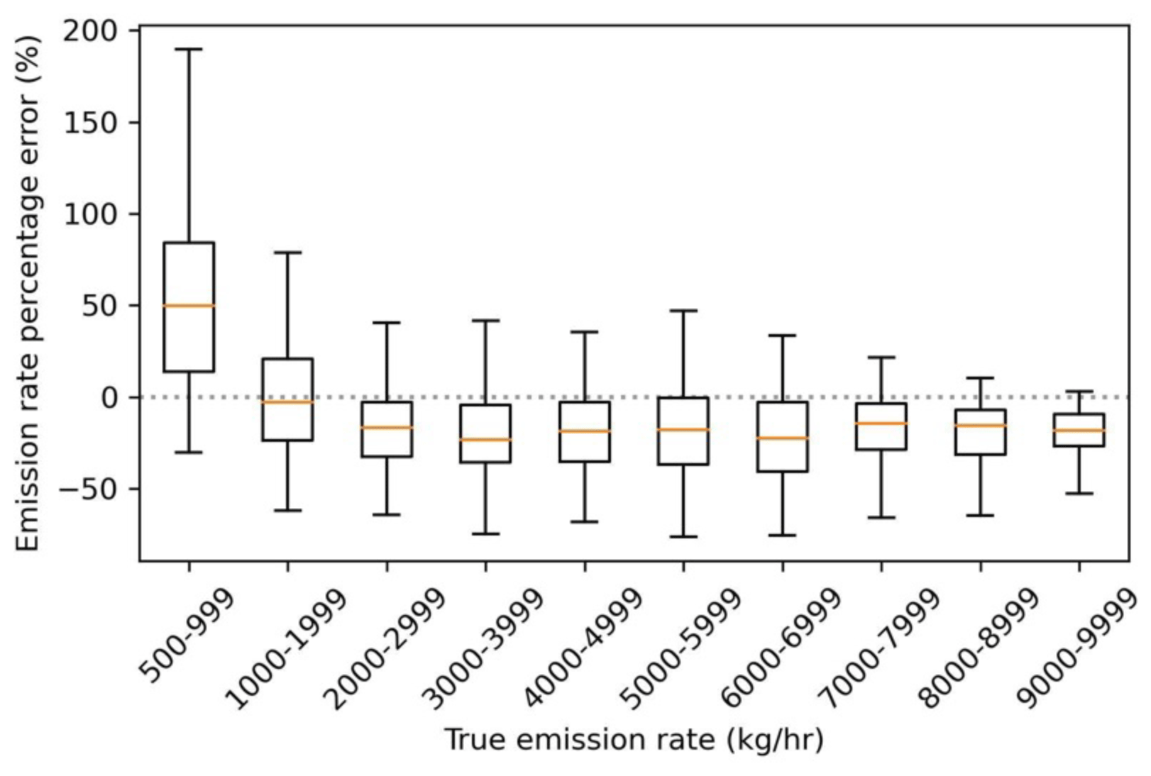
Figure 9Error in emission rate predictions from the deep learning model as a function of true emission rate. Positive values indicate predicted emission rates being larger than true emission rates. Top panel shows absolute emission rate error, and bottom panel shows percentage emission rate error.
3.2 Application to real-world images
The model was then tested on 40 PRISMA scenes obtained during 2020–2022 in the Korpeje oil field, Turkmenistan (37.9∘ N, 53.2∘ E–39.4∘ N, 55.2∘ E), a well-studied area with frequent methane point source emissions plumes (Irakulis-Loitxate et al., 2022). The images were normalised in the same way that the training, test, and validation images were. A total of 21 plumes were identified using the neural network from 15 different scenes, with predicted emission rates ranging from 1112–7615 kg h−1 (Fig. 10; Table S3).
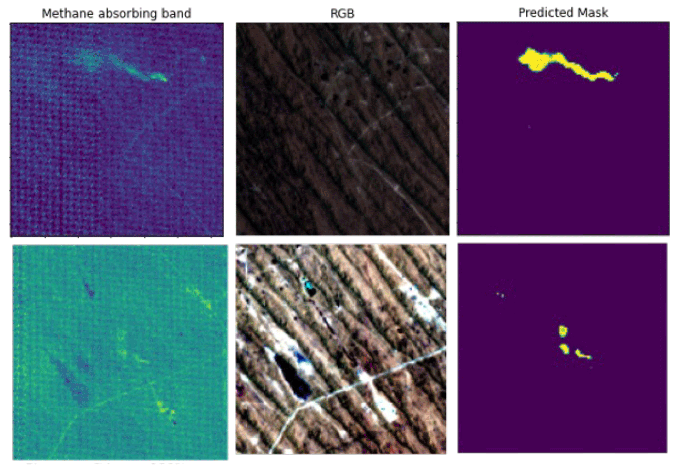
Figure 10Images of plumes detected by the neural network in the Korpeje oil field, Turkmenistan. Left panels depict physics-based methane retrievals, middle panels depict the RGB of the image, and the right panels depict the mask prediction by the neural network. The predicted emission rates are (top) 7615 and (bottom) 2370 kg h−1. RGB image courtesy of PRISMA (© Italian Space Agency).
Methane plume detection capability using the neural network was compared with using clustering and thresholding techniques. The DBSCAN clustering technique was used to estimate clusters based on the output from the PCA retrieval method (see Sect. 2.2). Out of the 21 plumes, 14 were found using the clustering and thresholding approach. The neural network model took roughly 1 min to make predictions of plume masks, methane concentrations, and emission rates of located plumes in an image of 1000×1000 pixels (900 km2 area) without the need for time-consuming human inspection typically needed for classical clustering approaches.
Reduction of methane emissions and hence identification of high emitters can have a considerable influence over the Earth's surface radiation budget and hence our efforts to mitigate climate change. Methods utilising classical approaches have had some success in detecting fossil fuel methane point sources and estimating their emissions, but the errors are high (roughly 50 % mean absolute error for emission rate predictions) if no accurate local wind speed information is available, and often time-consuming human judgement is necessary to separate plumes from surface effects. Within the pseudo-observation dataset produced in this study, only one-quarter of the images were deemed suitable to be analysed via visual inspection after using clustering algorithms. This was due to interference effects from surface features and demonstrates the limitation of this approach for detecting methane point source emissions. In comparison, only 7.7 % of the pseudo-observations were undetected by the neural network (Table 1). The binary prediction neural network presented in this study was able to accurately locate simulated methane point source plumes. From testing the neural network on a variety of images with and without simulated plumes, it achieved a precision and recall of 0.96 and 0.92, respectively. The estimates of emission rate did not require wind speed information, which is a major source for uncertainty in emission estimates in conventional approaches such as the IME method and had an average error of 23.7 %, which is considerably lower than that obtained from our classical method. The emission rate prediction error could possibly be further reduced with training on a larger dataset.
The approach used in this study differs from the approach by Jongaramrungruang et al. (2022), who directly predicted the emission rate from the satellite data without first estimating the plume mask. However, we found that excluding these stages dramatically worsened the model prediction, where the error in emission rate was greater than 50 %. The model architecture presented here utilises the maximum amount of information available from the training data. Possible explanations for why the model from Jongaramrungruang et al. (2022) was nevertheless successful could include the large training data volume available in their study (in the order of hundreds of thousands of images), which is an order of magnitude larger than that available in this study. This larger training volume may have enabled the neural network to make the link between plume shapes and emission rates. In addition, the spectral and spatial resolution of the aircraft imagery used in their study (AVIRIS-NG) is substantially higher than that of PRISMA. Finally, the input bands for this study totalled 38, whereas in the study of Jongaramrungruang et al., (2022), only one band was sufficient due to the low noise in the signal in the AVIRIS-NG data and high methane absorption in that band. Thus, it may have been easier for their neural network to learn features in the image due to lower noise present.
When producing the training data labels for plume masks, a constant threshold was chosen for what methane concentration constitutes a plume. However, the minimum methane concentration that is detectable likely varies depending on scene noise and brightness. Thus, more work is necessary to quantify the most appropriate threshold. However, precise estimates of the edges of a plume are of lesser importance than the initial identification of a plume and its corresponding emission rate. Additional improvements could be made with a larger volume and a greater variety of scenes used in training. This would greatly improve the performance of the model in different surface types and atmospheric conditions.
There is a noticeable bias present in the emission rate prediction errors (Figs. 8, 9), which was also evident in the study by Jongaramrungruang et al. (2022). This bias should be rectified, and future work is needed in fine-tuning the neural network training procedure to do so. Such adjustments could include modifying the emission rate loss function or the model architecture. The model was trained only on images with a single methane point source; thus, the model is not able to discriminate between emissions from different sources within a single 128×128-pixel image. The solution to this would be to add in training data with multiple sources and solve the instance segmentation problem using an appropriate architecture, such as Mask-RCNN (He et al., 2020). It is likely that the errors would be larger in general when using this approach owing to the increased noise present. Nevertheless, the key advantage of this approach is the speed with which methane plumes can be identified with little specialist training necessary.
In this study, we present a novel deep neural network model for identifying and quantifying methane point source emissions from PRISMA satellite data. PRISMA data have sufficient spectral and spatial resolution to identify methane plumes, while still having considerable spatial coverage, and are still in operation today. These factors make PRISMA an ideal tool for methane detection, and the deep neural network developed here has great potential to impact climate mitigation efforts. The model proved successful with both identification and quantification, but biases were present in the predictions. Rapid identification and quantification of methane point sources constitute a vital contribution to climate change mitigation, and the approach outlined here opens the door to the capability to automate methane plume detection. Our model was able to produce predictions on an area of 900 km2 over real PRISMA images in less than a minute. Such a capability will vastly reduce the time and costs associated with reducing anthropogenic methane emissions.
All of the data used in this study are freely available online. The WRF-LES model we used to make the methane release simulations is available for free online, as are all the PRISMA data used in this study to train the neural network. PRISMA data are available to download at http://prisma.asi.it/missionselect/ (Italian Space Agency, 2022, a sign-in is required). Codes for training the model are available at https://doi.org/10.5281/zenodo.7064085 (Joyce et al., 2022).
The supplement related to this article is available online at: https://doi.org/10.5194/amt-16-2627-2023-supplement.
PJ trained and deployed the neural network, was the lead writer of the manuscript, and produced the majority of figures. CRV produced training data from the simulated plumes. YH produced simulated plumes. AW produced some training data for simulated plumes and some figures for the paper. MG supervised the project and made edits to the manuscript. FHW had a supervisory role in the machine-learning direction of the work. MPC supervised the project. RBG produced some training data from the simulated plumes and carried out the clustering method for finding plumes. CW had a supervisory role and made edits to the manuscript. HB was the lead supervisor in the project and made edits to the manuscript.
The contact author has declared that none of the authors has any competing interests.
Publisher’s note: Copernicus Publications remains neutral with regard to jurisdictional claims in published maps and institutional affiliations.
We acknowledge funding from the Natural Environmental Research Council (NERC). Peter Joyce, Cristina Ruiz Villena, Alex Webb, Chris Wilson, Martyn P. Chipperfield, Yahui Huang, and Hartmut Boesch are funded via the UK National Centre for Earth Observation (grant nos. NE/R016518/1 and NE/N018079/1) and NERC MOYA project (grant no. NE/N015657/1). Manuel Gloor is funded by NERC POLYGRAM (grant no. NE/V006924/1). Part of this work was carried out at the Jet Propulsion Laboratory, California Institute of Technology, under a contract with the National Aeronautics and Space Administration (NASA). The project was carried out using original PRISMA products © Italian Space Agency (ASI); the products have been delivered under an ASI Licence to Use.
This research has been supported by the National Centre for Earth Observation (grant nos. NE/R016518/1, NE/N018079/1, NE/N015657/1, and NE/V006924/1).
This paper was edited by Alexander Kokhanovsky and reviewed by Luis Guanter and one anonymous referee.
Allen, D. T., Torres, V. M., Thomas, J., Sullivan, D. W., Harrison, M., Hendler, A., Herndon, S. C., Kolb, C. E., Fraser, M. P., and Hill, A. D.: Measurements of methane emissions at natural gas production sites in the United States, P. Natl. Acad. Sci. USA, 110, 17768–17773, 2013.
Alvarez, R. A., Zavala-Araiza, D., Lyon, D. R., Allen, D. T., Barkley, Z. R., Brandt, A. R., Davis, K. J., Herndon, S. C., Jacob, D. J., and Karion, A.: Assessment of methane emissions from the US oil and gas supply chain, Science, 361, 186–188, 2018.
Brandt, A. R., Heath, G. A., and Cooley, D.: Methane leaks from natural gas systems follow extreme distributions, Environ. Sci. Technol., 50, 12512–12520, 2016.
Chollet, F.: Keras: Deep Learning for humans, Release 2.12.0, GitHub [code], https://github.com/keras-team/keras (last access: 1 May 2023), 2015.
Cusworth, D. H., Jacob, D. J., Varon, D. J., Chan Miller, C., Liu, X., Chance, K., Thorpe, A. K., Duren, R. M., Miller, C. E., Thompson, D. R., Frankenberg, C., Guanter, L., and Randles, C. A.: Potential of next-generation imaging spectrometers to detect and quantify methane point sources from space, Atmos. Meas. Tech., 12, 5655–5668, https://doi.org/10.5194/amt-12-5655-2019, 2019.
Cusworth, D. H., Duren, R. M., Thorpe, A. K., Eastwood, M. L., Green, R. O., Dennison, P. E., Frankenberg, C., Heckler, J. W., Asner, G. P., and Miller, C. E.: Quantifying global power plant carbon dioxide emissions with imaging spectroscopy, AGU Advances, 2, e2020AV000350, https://doi.org/10.1029/2020AV000350, 2021a.
Cusworth, D. H., Duren, R. M., Thorpe, A. K., Olson-Duvall, W., Heckler, J., Chapman, J. W., Eastwood, M. L., Helmlinger, M. C., Green, R. O., and Asner, G. P.: Intermittency of large methane emitters in the Permian Basin, Environ. Sci. Tech. Let., 8, 567–573, 2021b.
Duren, R. M., Thorpe, A. K., Foster, K. T., Rafiq, T., Hopkins, F. M., Yadav, V., Bue, B. D., Thompson, D. R., Conley, S., and Colombi, N. K.: California's methane super-emitters, Nature, 575, 180–184, 2019.
Etminan, M., Myhre, G., Highwood, E., and Shine, K.: Radiative forcing of carbon dioxide, methane, and nitrous oxide: A significant revision of the methane radiative forcing, Geophys. Res. Lett., 43, 12614–612623, 2016.
Finch, D. P., Palmer, P. I., and Zhang, T.: Automated detection of atmospheric NO2 plumes from satellite data: a tool to help infer anthropogenic combustion emissions, Atmos. Meas. Tech., 15, 721–733, https://doi.org/10.5194/amt-15-721-2022, 2022.
Frankenberg, C., Thorpe, A. K., Thompson, D. R., Hulley, G., Kort, E. A., Vance, N., Borchardt, J., Krings, T., Gerilowski, K., Sweeney, C., Conley, S., Bue, B. D., Aubrey, A. D., Hook, S., and Green, R. O.: Airborne methane remote measurements reveal heavy-tail flux distribution in Four Corners region, P. Natl. Acad. Sci. USA, 113, 9734–9739, https://doi.org/10.1073/pnas.1605617113, 2016.
Galeazzi, C., Sacchetti, A., Cisbani, A., and Babini, G.: The PRISMA program, in: IGARSS 2008-2008 IEEE International Geoscience and Remote Sensing Symposium, Boston, USA, 7–11 July 2008, IEEE, IV-105–IV-108, https://doi.org/10.1109/IGARSS.2008.4779667, 2008.
Gordon, I., Rothman, L., Hargreaves, R., Hashemi, R., Karlovets, E., Skinner, F., Conway, E., Hill, C., Kochanov, R., and Tan, Y.: The HITRAN2020 molecular spectroscopic database, J. Quant. Spectrosc. Ra., 277, 107949, https://doi.org/10.1016/j.jqsrt.2021.107949, 2022.
Guanter, L., Irakulis-Loitxate, I., Gorroño, J., Sánchez-García, E., Cusworth, D. H., Varon, D. J., Cogliati, S., and Colombo, R.: Mapping methane point emissions with the PRISMA spaceborne imaging spectrometer, Remote Sens. Environ., 265, 112671, https://doi.org/10.1016/j.rse.2021.112671, 2021.
He, K., Zhang, X., Ren, S., and Sun, J.: Deep residual learning for image recognition, in: Proceedings of the IEEE conference on computer vision and pattern recognition, Las Vegas, USA, 27–30 June 2016, IEEE, 770–778, https://doi.org/10.1109/CVPR.2016.90, 2016.
He, K., Gkioxari, G., Dollar, P., and Girshick, R.: Mask R-CNN [J], IEEE T. Pattern Anal., 42, 386—397, 2020.
IEA: Key World Energy Statistics 2016, International Energy Agency (Ed.), https://www.iea.org/data-and-statistics/data-product/world-energy-statistics (last access: 15 March 2023), 2017.
Irakulis-Loitxate, I., Guanter, L., Maasakkers, J. D., Zavala-Araiza, D., and Aben, I.: Satellites Detect Abatable Super-Emissions in One of the World's Largest Methane Hotspot Regions, Environ. Sci. Technol., 56, 2143–2152, 2022.
Italian Space Agency (ASI): PRISMA data, ASI, http://prisma.asi.it/missionselect/, last access: 15 March 2022.
Jacob, D. J., Turner, A. J., Maasakkers, J. D., Sheng, J., Sun, K., Liu, X., Chance, K., Aben, I., McKeever, J., and Frankenberg, C.: Satellite observations of atmospheric methane and their value for quantifying methane emissions, Atmos. Chem. Phys., 16, 14371–14396, https://doi.org/10.5194/acp-16-14371-2016, 2016.
Jongaramrungruang, S., Frankenberg, C., Matheou, G., Thorpe, A. K., Thompson, D. R., Kuai, L., and Duren, R. M.: Towards accurate methane point-source quantification from high-resolution 2-D plume imagery, Atmos. Meas. Tech., 12, 6667–6681, https://doi.org/10.5194/amt-12-6667-2019, 2019.
Jongaramrungruang, S., Thorpe, A. K., Matheou, G., and Frankenberg, C.: MethaNet – An AI-driven approach to quantifying methane point-source emission from high-resolution 2-D plume imagery, Remote Sens. Environ., 269, 112809, https://doi.org/10.1016/j.rse.2021.112809, 2022.
Joyce, P., Ruiz Villena, C., Huang, Y., Webb, A., Gloor, M., Wagner, F. H., Chipperfield, M. P., Barrio Guilló, R., Wilson, C., and Boesch, H.: Using a deep neural network to detect methane point sources and quantify emissions from PRISMA hyperspectral satellite images, Version 1, Zenodo [code], https://doi.org/10.5281/zenodo.7064085, 2022.
Karion, A., Sweeney, C., Pétron, G., Frost, G., Michael Hardesty, R., Kofler, J., Miller, B. R., Newberger, T., Wolter, S., and Banta, R.: Methane emissions estimate from airborne measurements over a western United States natural gas field, Geophys. Res. Lett., 40, 4393–4397, 2013.
Krizhevsky, A., Sutskever, I., and Hinton, G. E.: Imagenet classification with deep convolutional neural networks, Commun. ACM, 60, 84–90, https://doi.org/10.1145/3065386, 2017.
Kuze, A., Suto, H., Nakajima, M., and Hamazaki, T.: Thermal and near infrared sensor for carbon observation Fourier-transform spectrometer on the Greenhouse Gases Observing Satellite for greenhouse gases monitoring, Appl. Optics, 48, 6716–6733, 2009.
LeCun, Y., Boser, B., Denker, J. S., Henderson, D., Howard, R. E., Hubbard, W., and Jackel, L. D.: Backpropagation applied to handwritten zip code recognition, Neural Comput., 1, 541–551, 1989.
Levelt, P. F., Hilsenrath, E., Leppelmeier, G. W., van den Oord, G. H., Bhartia, P. K., Tamminen, J., de Haan, J. F., and Veefkind, J. P.: Science objectives of the ozone monitoring instrument, IEEE T. Geosci. Remote, 44, 1199–1208, 2006.
Lorente, A., Borsdorff, T., Butz, A., Hasekamp, O., aan de Brugh, J., Schneider, A., Wu, L., Hase, F., Kivi, R., Wunch, D., Pollard, D. F., Shiomi, K., Deutscher, N. M., Velazco, V. A., Roehl, C. M., Wennberg, P. O., Warneke, T., and Landgraf, J.: Methane retrieved from TROPOMI: improvement of the data product and validation of the first 2 years of measurements, Atmos. Meas. Tech., 14, 665–684, https://doi.org/10.5194/amt-14-665-2021, 2021.
Matsugu, M., Mori, K., Mitari, Y., and Kaneda, Y.: Subject independent facial expression recognition with robust face detection using a convolutional neural network, Neural Networks, 16, 555–559, 2003.
Nugraha, B. T. and Su, S.-F.: Towards self-driving car using convolutional neural network and road lane detector, in: 2nd international conference on automation, cognitive science, optics, micro electro-mechanical system, and information technology (ICACOMIT), Jakarta, Indonesia, 23–24 October 2017, IEEE, 65–69, https://doi.org/10.1109/ICACOMIT.2017.8253388, 2017.
Ocko, I. B., Sun, T., Shindell, D., Oppenheimer, M., Hristov, A. N., Pacala, S. W., Mauzerall, D. L., Xu, Y., and Hamburg, S. P.: Acting rapidly to deploy readily available methane mitigation measures by sector can immediately slow global warming, Environ. Res. Lett., 16, 054042, https://doi.org/10.1088/1748-9326/abf9c8, 2021.
Oh, K.-S. and Jung, K.: GPU implementation of neural networks, Pattern Recogn., 37, 1311–1314, 2004.
Parker, R. J., Webb, A., Boesch, H., Somkuti, P., Barrio Guillo, R., Di Noia, A., Kalaitzi, N., Anand, J. S., Bergamaschi, P., Chevallier, F., Palmer, P. I., Feng, L., Deutscher, N. M., Feist, D. G., Griffith, D. W. T., Hase, F., Kivi, R., Morino, I., Notholt, J., Oh, Y.-S., Ohyama, H., Petri, C., Pollard, D. F., Roehl, C., Sha, M. K., Shiomi, K., Strong, K., Sussmann, R., Té, Y., Velazco, V. A., Warneke, T., Wennberg, P. O., and Wunch, D.: A decade of GOSAT Proxy satellite CH4 observations, Earth Syst. Sci. Data, 12, 3383–3412, https://doi.org/10.5194/essd-12-3383-2020, 2020.
Ronneberger, O., Fischer, P., and Brox, T.: U-net: Convolutional networks for biomedical image segmentation, in: International Conference on Medical image computing and computer-assisted intervention, Munich, Germany, 5–9 October 2015, 234–241, https://doi.org/10.1007/978-3-319-24574-4_28 2015.
Saunois, M., Stavert, A. R., Poulter, B., Bousquet, P., Canadell, J. G., Jackson, R. B., Raymond, P. A., Dlugokencky, E. J., Houweling, S., Patra, P. K., Ciais, P., Arora, V. K., Bastviken, D., Bergamaschi, P., Blake, D. R., Brailsford, G., Bruhwiler, L., Carlson, K. M., Carrol, M., Castaldi, S., Chandra, N., Crevoisier, C., Crill, P. M., Covey, K., Curry, C. L., Etiope, G., Frankenberg, C., Gedney, N., Hegglin, M. I., Höglund-Isaksson, L., Hugelius, G., Ishizawa, M., Ito, A., Janssens-Maenhout, G., Jensen, K. M., Joos, F., Kleinen, T., Krummel, P. B., Langenfelds, R. L., Laruelle, G. G., Liu, L., Machida, T., Maksyutov, S., McDonald, K. C., McNorton, J., Miller, P. A., Melton, J. R., Morino, I., Müller, J., Murguia-Flores, F., Naik, V., Niwa, Y., Noce, S., O'Doherty, S., Parker, R. J., Peng, C., Peng, S., Peters, G. P., Prigent, C., Prinn, R., Ramonet, M., Regnier, P., Riley, W. J., Rosentreter, J. A., Segers, A., Simpson, I. J., Shi, H., Smith, S. J., Steele, L. P., Thornton, B. F., Tian, H., Tohjima, Y., Tubiello, F. N., Tsuruta, A., Viovy, N., Voulgarakis, A., Weber, T. S., van Weele, M., van der Werf, G. R., Weiss, R. F., Worthy, D., Wunch, D., Yin, Y., Yoshida, Y., Zhang, W., Zhang, Z., Zhao, Y., Zheng, B., Zhu, Q., Zhu, Q., and Zhuang, Q.: The Global Methane Budget 2000–2017, Earth Syst. Sci. Data, 12, 1561–1623, https://doi.org/10.5194/essd-12-1561-2020, 2020.
Sherwin, E. D., Rutherford, J. S., Chen, Y., Aminfard, S., Kort, E. A., Jackson, R. B., and Brandt, A. R.: Single-blind validation of space-based point-source detection and quantification of onshore methane emissions, Sci. Rep.-UK, 13, 3836, https://doi.org/10.1038/s41598-023-30761-2, 2023.
Stocker, T., Qin, D., Plattner, G.-K., Tignor, M. M. B., Allen, S. K., Boschung, J., Nauels, A., Xia, Y., Bex, V., and Midgley, P. M.: Climate Change 2013: The Physical Science Basis. Contribution of Working Group I to the Fifth Assessment Report of the Intergovernmental Panel on Climate Change, IPCC, Geneva, 2013.
Thorpe, A. K., Frankenberg, C., and Roberts, D. A.: Retrieval techniques for airborne imaging of methane concentrations using high spatial and moderate spectral resolution: application to AVIRIS, Atmos. Meas. Tech., 7, 491–506, https://doi.org/10.5194/amt-7-491-2014, 2014.
Varon, D. J., Jacob, D. J., McKeever, J., Jervis, D., Durak, B. O. A., Xia, Y., and Huang, Y.: Quantifying methane point sources from fine-scale satellite observations of atmospheric methane plumes, Atmos. Meas. Tech., 11, 5673–5686, https://doi.org/10.5194/amt-11-5673-2018, 2018.
Varon, D. J., Jervis, D., McKeever, J., Spence, I., Gains, D., and Jacob, D. J.: High-frequency monitoring of anomalous methane point sources with multispectral Sentinel-2 satellite observations, Atmos. Meas. Tech., 14, 2771–2785, https://doi.org/10.5194/amt-14-2771-2021, 2021.
Wallach, I., Dzamba, M., and Heifets, A.: AtomNet: a deep convolutional neural network for bioactivity prediction in structure-based drug discovery, arXiv [preprint], https://doi.org/10.48550/arXiv.1510.02855, 10 October 2015.
Zavala-Araiza, D., Lyon, D. R., Alvarez, R. A., Davis, K. J., Harriss, R., Herndon, S. C., Karion, A., Kort, E. A., Lamb, B. K., and Lan, X.: Reconciling divergent estimates of oil and gas methane emissions, P. Natl. Acad. Sci. USA, 112, 15597–15602, 2015.
Zavala-Araiza, D., Alvarez, R. A., Lyon, D. R., Allen, D. T., Marchese, A. J., Zimmerle, D. J., and Hamburg, S. P.: Super-emitters in natural gas infrastructure are caused by abnormal process conditions, Nat. Commun., 8, 1–10, 2017.