the Creative Commons Attribution 4.0 License.
the Creative Commons Attribution 4.0 License.
 | 07 Jun 2023
Cloud mask algorithm from the EarthCARE Multi-Spectral Imager: the M-CM products
Sebastian Bley
Stefan Horn
Hartwig Deneke
Andi Walther
The EarthCARE (Earth Clouds, Aerosols and Radiation Explorer) satellite mission will provide new insights into aerosol–cloud–radiation interactions by means of synergistic observations of the Earth's atmosphere from a collection of active and passive remote sensing instruments, flying on a single satellite platform. The Multi-Spectral Imager (MSI) will provide visible and infrared images in the cross-track direction with a 150 km swath and a pixel sampling at 500 m. The suite of MSI cloud algorithms will deliver cloud macro- and microphysical properties complementary to the vertical profiles measured from the Atmospheric Lidar (ATLID) and the Cloud Profiling Radar (CPR) instruments. This paper provides an overview of the MSI cloud mask algorithm (M-CM) being developed to derive the cloud flag, cloud phase and cloud type products, which are essential inputs to downstream EarthCARE algorithms providing cloud optical and physical properties (M-COP) and aerosol optical properties (M-AOT). The MSI cloud mask algorithm has been applied to simulated test data from the EarthCARE end-to-end simulator and satellite data from the Moderate Resolution Imaging Spectroradiometer (MODIS) as well as from the Spinning Enhanced Visible InfraRed Imager (SEVIRI). Verification of the MSI cloud mask algorithm to the simulated test data and the official cloud products from SEVIRI and MODIS demonstrates a good performance of the algorithm. Some discrepancies are found, however, for the detection of thin cirrus clouds over bright surfaces like desert or snow. This will be improved by tuning of the thresholds once real observations are available.
- Article
(9328 KB) - Full-text XML
- BibTeX
- EndNote


Clouds cover about 70 % of our Earth's surface and play an important role in the global radiation and energy budgets. The influence of clouds on radiative fluxes exhibits a complex dependency on cloud type, phase and geometric height as well as their optical and microphysical properties, potentially introducing significant radiative feedbacks in response to climate change. The Intergovernmental Panel on Climate Change (IPCC) Sixth Assessment Report summarizes the current state of knowledge, concluding that clouds are expected to amplify global warming as a result of an increase in high-level clouds and a reduction in low-level clouds (IPCC, 2021). The report provides a best estimate of the net cloud feedback, having a positive value of 0.42 W m−2. While the uncertainty related to cloud feedbacks has been halved compared to the previous Fifth Assessment Report, the response of clouds to a warming Earth remains one of the biggest challenges in our understanding of the climate system.
The determination of cloud, atmospheric and surface properties from multi-spectral satellite imagery relies on the accurate discrimination of cloudy and cloud-free pixels. This discrimination is typically done by a cloud mask algorithm as the first step in a processing chain of satellite imagery. If for instance cloudy areas are misclassified as clear or vice versa, this could negatively impact subsequent retrievals of aerosol or cloud optical properties, which underlies the importance of an accurate cloud-masking algorithm. Different comparison studies and intercomparison studies have been done like the Cloud Masking Intercomparison eXercise (CMIX) to evaluate the cloud-masking algorithms (Skakun et al., 2022; Zekoll et al., 2021). These techniques are mostly based on two general assumptions, namely that clouds appear brighter in solar channels, due to the strong reflection of sunlight, and colder in infrared channels relative to cloud-free surfaces, due to the decrease in atmospheric temperature with height. In addition, discrimination of clouds from cloud-free regions is commonly based on a variety of spectral features, spatial structure measures or temporal characteristics in time series because clouds are often more variable than the underlying surface (Saunders and Kriebel, 1988).
Operational cloud mask algorithms generally combine a variety of individual tests by means of a decision tree, as no single test is able to achieve a sufficient accuracy for the diversity of clouds and atmospheric conditions encountered globally (e.g., Saunders and Kriebel, 1988). An alternative is the use of fuzzy-logic-based or Bayesian schemes to combine tests to yield a confidence value or probability for the classification (e.g., Ackerman et al., 1998; Hollstein et al., 2015). More recently, convolutional neural networks have been applied to discriminate between different land surfaces, ocean, clouds and cloud shadows (Mateo-García et al., 2017; Li et al., 2019; Hughes and Kennedy, 2019). Such cloud-masking approaches are often applied to high-resolution satellite images (e.g., Landsat, Sentinel-2) and require large training datasets. In practice, these training datasets have to be created manually, and the significant effort required for establishing high-quality training datasets and validating their performance has so far not led to operational application in global-scale long-term cloud climate data records. Rossow and Garder (1993) classify the different tests used in cloud mask algorithms into radiance threshold tests, spatial variance tests, temporal variance tests and tests using independent datasets to estimate clear-sky radiances. The performance of these tests strongly depends on the satellite sensor specifications including spatial, spectral and temporal resolution.
The International Satellite Cloud Climatology Project (ISCCP; Schiffer and Rossow, 1983) was the earliest effort to provide a comprehensive global cloud climatology from multi-spectral meteorological satellite imagers. Its cloud detection algorithm is described in Rossow and Garder (1993) and is based on a combination of static and dynamic threshold tests for one window channel in the visible and one window channel in the thermal infrared wavelength range. This choice was made based on the limited availability of channels from early geostationary satellites, specifically the Meteosat, GMS (Geostationary Meteorological Satellite) and GOES (Geostationary Operational Environmental Satellite) series.
Based on the Advanced Very High Resolution Radiometer (AVHRR) which has been flown on NOAA's polar-orbiting satellites since the early 1980s, the APOLLO (AVHRR Processing scheme Over cLoud, Land, and Ocean) cloud detection scheme used both static and dynamic threshold tests. The availability of additional spectral channels was used in particular to improve nighttime cloud detection performance. Dynamic thresholds were derived from a histogram-based scene analysis (Saunders and Kriebel, 1988; Strabala et al., 1994).
A new milestone in instrumental capabilities was reached by the Moderate Resolution Imaging Spectroradiometer (MODIS) instrument, providing observations in 36 spectral channels from NASA's Earth Observing System satellites Terra and Aqua, launched in 1999 and 2002, respectively. The operational cloud mask product for MODIS considers the spectral information from 19 of these channels (Ackerman et al., 2002; Platnick et al., 2003). While several spectral tests are similar to those used by the APOLLO and ISCCP cloud detection schemes, the availability of channels in water vapor and CO2 absorption bands enabled an improved cloud detection in particular for thin high-level clouds and for polar night conditions (e.g., Liu et al., 2004; Nakajima et al., 2011).
EarthCARE, the Earth Clouds, Aerosols and Radiation Explorer, is a joint European and Japanese mission and part of ESA's Living Planet program (Illingworth et al., 2015; Wehr et al., 2023). The mission objective is to improve our understanding of aerosol–cloud–radiation interactions and the role of aerosols and clouds in the Earth radiation budget. While observation of clouds have gradually improved over the past decades, the launch of the EarthCARE satellite is expected to bring a breakthrough by means of its novel observational capabilities. To achieve the mission objective, accurate and simultaneous measurements of microphysical and optical properties of aerosol and clouds together with solar and infrared radiation fluxes are crucial. EarthCARE will offer the unique opportunity to collect these observations at a global scale due to its polar orbit. The satellite will carry an exceptional collection of active and passive remote sensing instruments, flying on a single satellite platform in an orbit at an altitude of 393 km. The instruments include the Atmospheric Lidar (ATLID), the Cloud Profiling Radar (CPR), the Multi-Spectral Imager (MSI) and the Broad-Band Radiometer (BBR).
This paper describes the algorithm used to produce the cloud flag, type and phase products based alone on MSI observations. The approaches selected for EarthCARE's MSI cloud mask (M-CM) products relies on the research on and experience with cloud-masking approaches during the past 40 years since the start of the satellite era. It exploits the full spectral information content of the MSI instrument (e.g., the cloud type is determined using 3D histograms of the VIS, visible; SWIR-2, short-wave infrared; and TIR-2, thermal infrared, channels). It is, however important to realize that its performance is also determined by the selection of four solar and three infrared channels for MSI, having central wavelengths of 670 nm (VIS), 865 nm (NIR, near infrared), 1650 nm (SWIR-1), 2210 nm (SWIR-2), 8.8 µm (TIR-1), 10.8 µm (TIR-2) and 12.0 µm (TIR-3). Given this specification, MSI's capabilities and sensitivity is more similar to that of AVHRR than of MODIS. In particular, no channels within absorption bands of atmospheric gases are available. Reflectances in the solar channels are used to detect clouds by means of a visible reflectance test and a reflectance ratio test. The visible reflectance test assumes that the reflectance of clouds exceeds the reflectance of cloud-free surfaces, with the exception of highly reflective surfaces. The reflectance ratio test compares the ratio of the reflectances of two shortwave channels to thresholds. Complementing the solar channel tests, a brightness temperature test uses information from the thermal infrared (TIR) channels to detect clouds based on the assumption that the brightness temperature of clouds is significantly lower than the brightness temperature of cloud-free pixels.
The estimation of the expected difference in cloud-free brightness temperatures for the three infrared channels is an important aspect for the accuracy of cloud detection. This difference depends on differences in atmospheric absorption (water vapor) and surface emissivity. Therefore, scene-dependent lookup tables or online radiative transfer simulations have to be elaborated to determine suitable thresholds. All tests yield a probability that a pixel is cloud-free. Some of the individual tests are however not independent of each other because they rely on similar channels and principles. Hence, the resulting probabilities of those tests are combined. For every 500 m resolution pixel of the 150 km wide MSI swath, the M-CM products provide a classification whether it is cloud-covered or cloud-free as the final output. Additionally, for the cloudy pixels, the cloud type and cloud phase of the uppermost cloud layer will be reported.
This paper is structured as follows. Section 2 describes the algorithms for deriving the operational Level 2 M-CM products, which comprise a binary cloud flag, cloud phase and cloud type as well as confidence statistics. The verification of the algorithm using MODIS and Meteosat Second Generation (MSG) SEVIRI scenes as well as synthetic test data from the EarthCARE end-to-end simulator (Donovan et al., 2023) is provided in Sect. 3. Comprehensive comparisons between the operational M-CM product and the synthetic test fields are presented in Appendix A. The data processing chain including the role of M-CM is explained in more detail in Eisinger et al. (2023).
The MSI cloud product processor (M-CLD) provides algorithms for calculation of the cloud flag; cloud phase; cloud type; cloud optical depth; cloud particle size; cloud water path; and cloud top temperature, pressure and height. The processor consists of two main parts, which are sequentially processed. First is the cloud mask (M-CM), which is mandatory for the other cloud optical and physical properties (M-COP). The present paper describes the cloud mask processor (M-CM), which is schematically shown in Fig. 1.
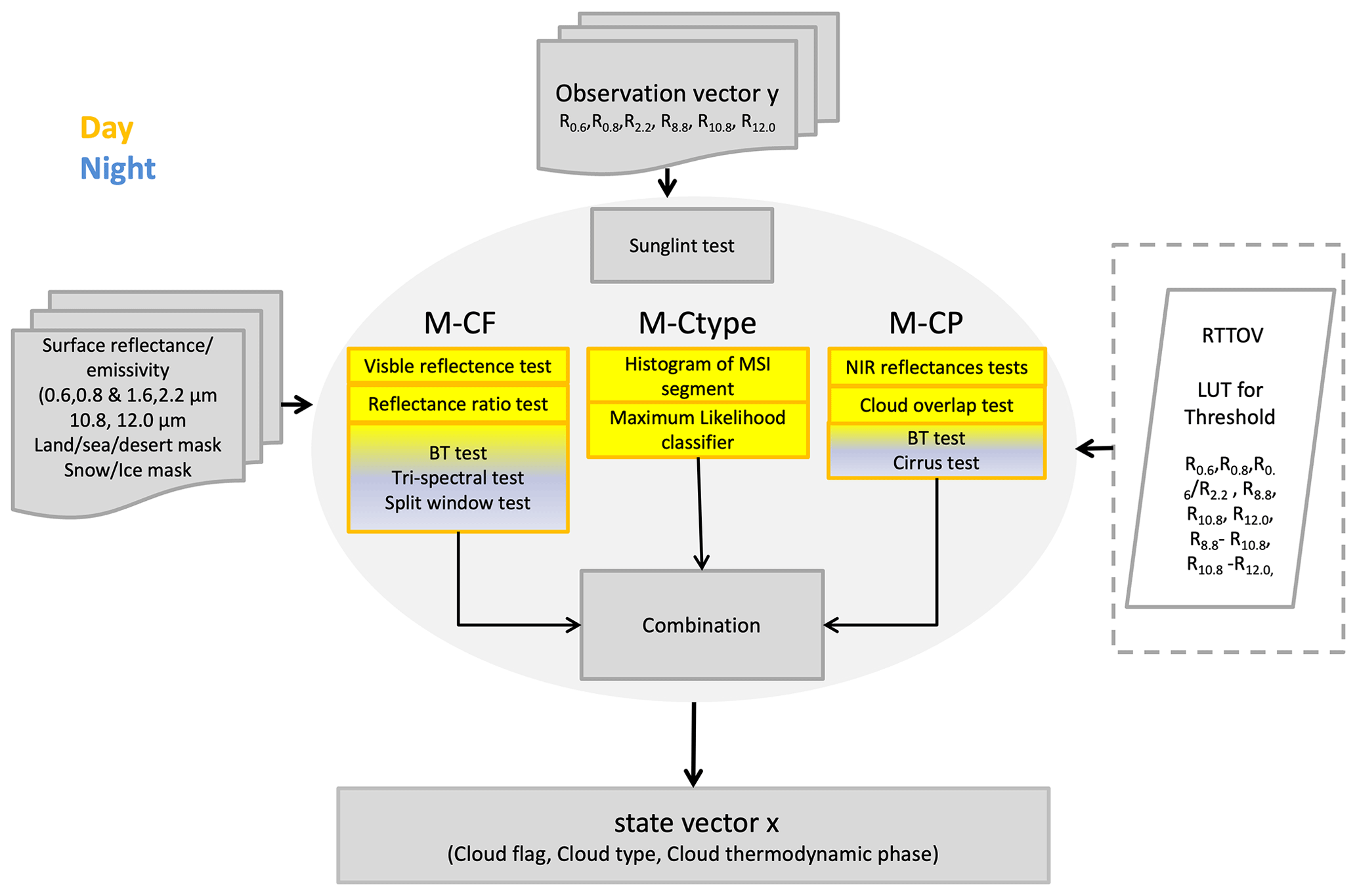
Figure 1Schematic of the main components of the M-CM algorithm. BT: brightness temperature, LUT: lookup table.
The algorithm starts with the calculation of the reflectances at the top of the atmosphere in the shortwave channels. The reflectances (ρi) of each channel i are obtained from the measured radiance (L) and the solar irradiance E0 as
with the sun zenith angle θ0, the viewing zenith angle θ and the relative azimuth angle ϕ. An important input for the algorithm is the day/night flag. The daytime condition is considered for a certain pixel of the sun zenith angle θ0<80∘. Additionally, the sunglint angle θr is calculated over ocean as
If θr<36∘, the pixel is flagged with sunglint provided in the surface flag.
2.1 M-CF: binary cloud flag
The algorithm derives a cloud mask by applying individual threshold tests to brightness temperatures and reflectances of individual channels. The threshold tests and the way that results are combined are adapted from the MODIS cloud mask algorithm (Ackerman et al., 2002). The thresholds rely on the assumption that spectral signatures of cloud-free pixels and pixels covered by different cloud types differ. As the thresholds vary globally, only the upper (cloudy) and lower (cloud-free) limits of the thresholds are defined, and a linear function is used to determine the probability that a cloud is really present based on how close the observation is to the limits. Furthermore, the probability of being cloud-free from the applied tests is combined to an overall probability which may provide, in combination with the number of applied tests, a measure of the confidence of the result. From the overall probability a binary cloud mask indicating if a pixel is cloudy or not is derived with four levels of confidence: clear, probably clear, probably cloudy and cloudy.
2.1.1 Visible reflection tests
The visible reflectance test compares the reflectance in the 0.67 µm channel or the reflectance in the 0.865 µm channel with surface-dependent thresholds (Fig. 2). These thresholds are initially taken from the MODIS cloud mask algorithm. These thresholds have been tuned based on simulated MSI properties, while further adaptions are planned at a later stage, when actual MSI data will become available. If the reflectance exceeds the upper threshold, pixels are assumed to be very likely cloudy. Pixels with reflectances below the lower threshold are classified with high confidence as cloud-free. The pixels in between are classified by calculating probability functions, as described in Sect. 2.1.3.
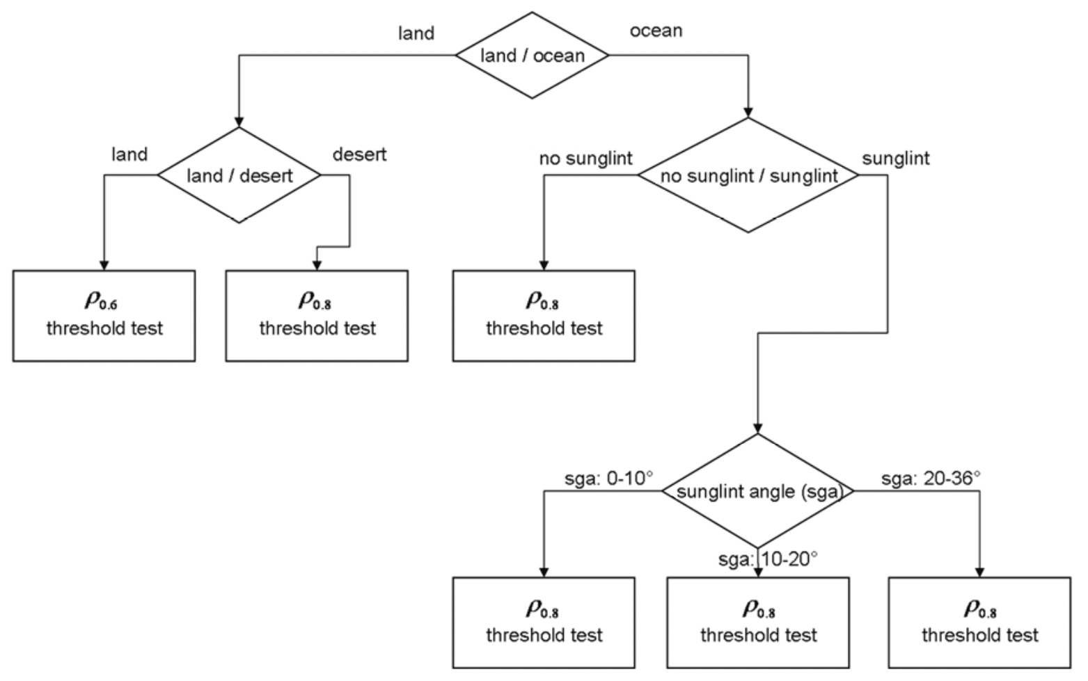
The upper and the lower thresholds differ for land, desert and ocean pixels outside the sunglint region and ocean pixels in the sunglint region (Fig. 2). Whereas the thresholds are fixed for the first three classes, they depend on the sunglint angle in the sunglint region. Over land the test applies the reflectance in the 0.67 µm channel, while over desert the reflectance in the 0.865 µm channel is used. Ocean pixels located outside the sunglint region are classified by using the reflectance in the 0.865 µm channel. Ocean pixels affected by sunglint also apply thresholds based on the 0.865 µm channel, but the thresholds are calculated depending on the sunglint angle (see Eq. 2). The lower and upper thresholds of the 0.865 µm tests depend on predefined limits of sunglint angles between 0–10, 10–20 and 20–36∘ (Fig. 2).
2.1.2 Reflectance ratio test
The reflectance ratio test is applied to daytime pixels over oceans and land surfaces with low reflectivities. Therefore, the land pixels are classified in surfaces with high reflectivity like desert, polar and semi-arid regions and low reflectivity. Over ocean the reflectance ratio test can be applied as well in the sunglint region. The test score is the ratio of the reflectance in the 0.865 µm channel and the reflectance in the 0.67 µm channel. If the test score is smaller than the lower threshold, the pixel is classified with high confidence as cloud-free. A test score larger than the upper threshold results in labeling the pixel with high confidence as cloudy. For pixels with values in between, the confidence level is calculated in a linear way. Upper and lower thresholds are defined for ocean pixels outside and inside the sunglint region, respectively.
For a land pixel indicated by the application mask as appropriate, the test score is a modified GEMI (Global Environmental Monitoring Index) first described by Pinty and Verstraete (1992). It is calculated as
with
If m_gemi is greater than m_gemiclear, the pixel is classified with high confidence as clear, and if m_gemi is lower than m_gemicloudy, the pixel is assumed with high confidence to be cloudy. If values in between appear, then the confidence level of being clear is calculated by a linear approach.
2.1.3 Brightness temperature tests
We use two different approaches for the brightness temperature tests, one using simple thresholds and the other one applying brightness temperature differences between different infrared channels for the separation between cloudy and cloud-free pixels. The first simple threshold test is applied on the 10.85 µm channel for all surface types during nighttime. The pixels is identified as cloudy if
where the clear-sky brightness temperature T10.8_cs, at top of the atmosphere, is calculated with the IR radiative transfer model (RTTOV; Saunders et al., 1999) on the grid of the auxiliary meteorological (X-MET) data and then interpolated to the geolocation and measurement time of the MSI pixel. The X-MET dataset provides additional meteorological model parameters required for the processing (Eisinger et al., 2023). Details about the RTTOV forward simulation are described in Hünerbein et al. (2023). If T10.8_cs is larger than T10.8, the pixel is assumed to be cloudy. The probability of being cloud-free is calculated by assuming a linear probability function. The tri-spectral window brightness temperature difference test (at 8.8, 10.8 and 12.0 µm) is only applied to water surfaces during daytime. The brightness temperatures at 10.8 and at 12.0 µm are used to detect thin cirrus clouds and cloud edges, which are characterized by a higher brightness temperature difference (10.8–12.0 µm) than a cloud-free surface. The pixel is detected as cloudy if
where Tdiff1_cs is calculated with RTTOV for each pixel for clear-sky conditions. By use of the temperature differences at 8.8–10.8 µm, thin cirrus clouds over all surface conditions can be detected. In addition to Eq. (6) if the difference is relatively high compared to the clear-sky condition, then the pixel is classified as cloudy if
The probability of being cloud-free is calculated by assuming a linear probability function. The same applies for the tri-spectral brightness temperature difference test. Further investigation is needed to define the base threshold, which is strongly dependent on surface and water vapor.
2.1.4 Estimation of confidence level
The results of all tests are combined in a two-step procedure for determination of the confidence level (Fig. 3). In the first step the overall probability for each pixel from the tests applying reflectances is derived because these tests are not independent. This is accomplished by finding the minimum probability Gi of being cloudy in both tests. In the next step the probability from the brightness temperature test and the intermediate result from the reflectance tests are combined by calculation of the square root of the multiplied values if multiple valid test results are available:
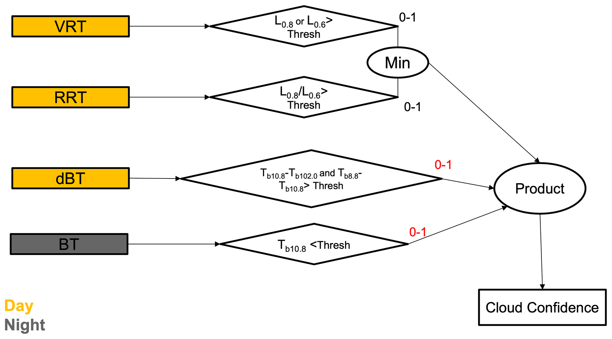
Figure 3Four groups of cloud tests to determine cloud confidences. VRT: visible reflection tests, RRT: reflectance ratio test, dBT: brightness temperature difference.
Otherwise the final result consists of the valid test result or is undefined. The square root of the multiplied probabilities of a pixel being clear ensures that the overall result does not tend to cloudy pixels as would be the case if results were solely multiplied. This approach is considered clear-sky conservative.
2.2 M-Ctype: cloud types
The algorithm applies a maximum-likelihood classifier to reflectances and brightness temperatures at VIS, SWIR-2 and TIR-2. Before the algorithm assigns a specific cloud type for a certain pixel, the dataset needs to be trained to acquire statistics for predefined cloud classes. This procedure is described in the following section.
2.2.1 Cloud type training using MODIS
A large number of MODIS scenes are used to learn statistics for nine predefined cloud classes (from thin to thick clouds, high, medium and low clouds) and one cloud-free class, either over sea, land or desert and separated into stripes of 15∘ latitude. Nine cloud classes are categorized by using the MODIS cloud top height and cloud optical thickness based on the ISCCP cloud classification schemes (Rossow and Schiffer, 1999). From these scenes, the mean vector and covariance matrix are calculated for all cloud classes, with one cloud-free class from the visible channel, the shortwave infrared channel and the infrared channel, and saved in a lookup table.
The region, season and surface are identified for each pixel. The regions are defined by a circle of latitude in 15∘ steps. The pixels are separated into four seasons (winter, spring, summer and fall) based on the month (Fig. 4). The surfaces are separated with the land–sea mask into land, water and desert pixels. The nine ISCCP cloud classes can be clearly distinguished between cirrus, cirrostratus, deep convection, altocumulus, altostratus, nimbostratus, cumulus, stratocumulus and stratus. Also a clear-sky class is defined for the different surface types, regions and seasons (not shown in Fig. 4). The statistics are then used to assign each pixel in the measured scene to a certain class by applying a maximum-likelihood classifier. The algorithm assumes either a completely cloud-covered or completely cloud-free pixel and does not take sub-pixel clouds into account.
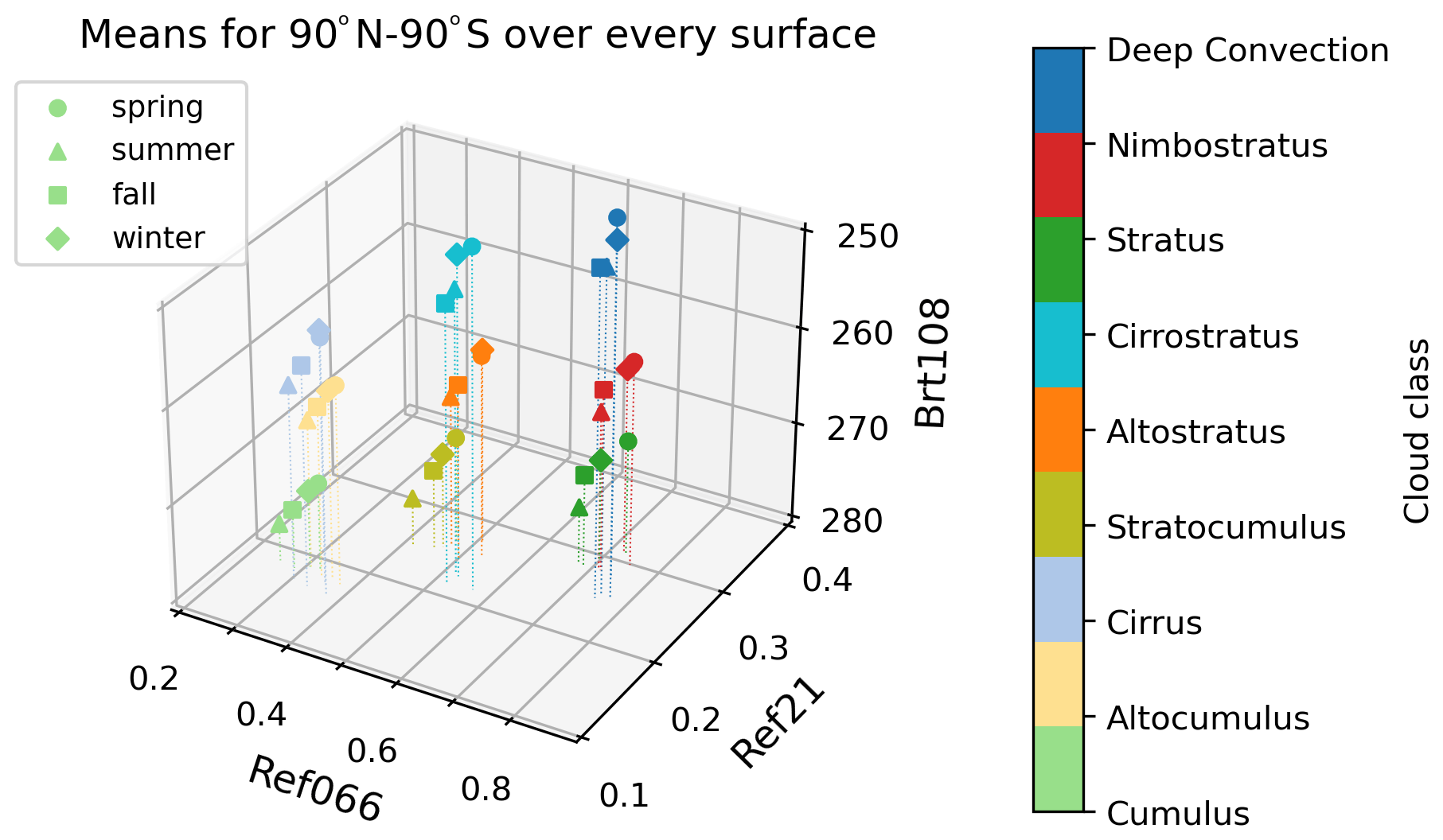
Figure 4Observed reflectances (Ref) and brightness (Brt) temperatures at VIS, SWIR-2 and TIR-2 (MODIS) for the nine ISCCP cloud classes (cirrus, cirrostratus, deep convection, altocumulus, altostratus, nimbostratus, cumulus, stratocumulus and stratus) and seasonal separation.
2.2.2 Maximum-likelihood classifier
The probability is computed for each MSI pixel to all individual classes by means of a maximum-likelihood classifier. A pixel is assigned to class j if the likelihood of class j is the greatest among the 9+1 classes which are relevant for the respective surface. The maximum likelihood is found by
with x being the vector of properties (reflectances and brightness temperature) in the considered channels, mi being the mean vector of class i, ∑i being the covariance matrix and p being the number of maximum-likelihood classes for the respective surface. Though a maximum-likelihood classifier that does not assign a class when the maximum-probability value falls below a certain probability also exists, the classifier applied here is a hard classifier assigning a class to every pixel with valid radiation data independent of the magnitude of the maximum probability. The reliability of a maximum-likelihood classification result depends on the probability for the assigned class i and the probability for the next class j derived as . The next class is determined by minimizing argmin . The assignments to the nine cloud classes and the clear-sky class are determined for all pixels.
2.3 M-CP: cloud phase
The discrimination of the thermodynamic phase at the cloud top is based on the spectral absorption differences in ice and water clouds between the visible (0.67 µm) and the shortwave infrared (1.65 µm) as well as the brightness temperatures at 8.8, 10.8 and 12.0 µm. The cloud phase categories of the M-CP algorithm include liquid water, ice, supercooled mixed phase and cloud overlap (e.g., multi-layer clouds). The M-CP retrieval closely follows the approach applied to AVHRR and the Visible Infrared Imaging Radiometer Suite (VIIRS) (Pavolonis et al., 2005; Pavolonis and Heidinger, 2004) as well as for MODIS (Strabala et al., 1994). The algorithm consists of several spectral threshold tests applied to the reflectances from the VIS, SWIR and TIR channels. The thresholds are adapted from the corresponding AVHRR channels based on Pavolonis et al. (2005). The fine tuning of these thresholds will be done with the whole measurements suite of EarthCARE at nadir. The algorithm starts with a series of threshold tests based on TIR-2, which follows the physical assumption that the cloud top phase depends on the cloud top temperature. The liquid water category includes clouds of liquid water droplets that have a temperature greater than 273.16 K measured by TIR-2. Only non-opaque cirrus clouds can also fall into that category. To detect semitransparent cirrus clouds over optically thick water clouds, a cloud overlap test is done. The cloud overlap detection uses the VIS, TIR-2 and TIR-3 channels. This method is adapted from the AVHRR algorithm explained by Pavolonis and Heidinger (2004). The underlying physical theory is that the VIS reflectance will not change much when having an overlapping thin cirrus cloud over a thick water cloud, while the temperature difference between both clouds results in a brightness temperature difference in the IR window channels that is larger than predicted by radiative transfer calculations. A certain pixel is defined as an ice cloud if the BT at 10.8 µm < 233.16 K and the overlap test fails. Supercooled mixed-phase cloud pixels are assumed based on threshold tests with the BT at 10.8 µm between 233.16 and 273.16 K. During daytime conditions, additional tests are applied using the SWIR-1 channel, which improves the detection of overlapping and cirrus clouds.
2.4 Surface flag
The surface flag distinguishes between water, land, desert, vegetation, snow, sea ice, sunglint and undefined. While the surface types water, land, desert and sunglint are used as input for the M-CM algorithm, the types vegetation and snow are calculated for the cloud-free pixels only, by using the normalized difference vegetation index (NDVI) and the normalized difference snow index (NDSI). The NDVI is the normalized ratio of the difference in reflectance at NIR and VIS based on the red edge feature of the vegetation.
The NDSI is the normalized ratio of the difference in reflectance at VIS and SWIR-1. The atmosphere is transparent at both wavelengths, while snow is very reflective at VIS and not reflective at SWIR-1.
The algorithm distinguishes between sparse vegetation/ocean and dense vegetation with the NDVI and identifies snow surfaces with the NDSI.
2.5 M-CM quality flags
The M-CM quality flags provide pixel-based quality information for the cloud flag, the cloud type and the cloud phase products. The quality flags distinguish between high, medium, low and poor quality. These measures do not represent probabilities but rather the number of tests which have been executed for the associated pixel, the consistency among the products or the surface flag. The definitions of the individual quality flags are provided in Table 1.
Table 1Definitions of pixel-based quality flags (high, medium, low, poor) for the cloud flag, the cloud type and the cloud phase products.
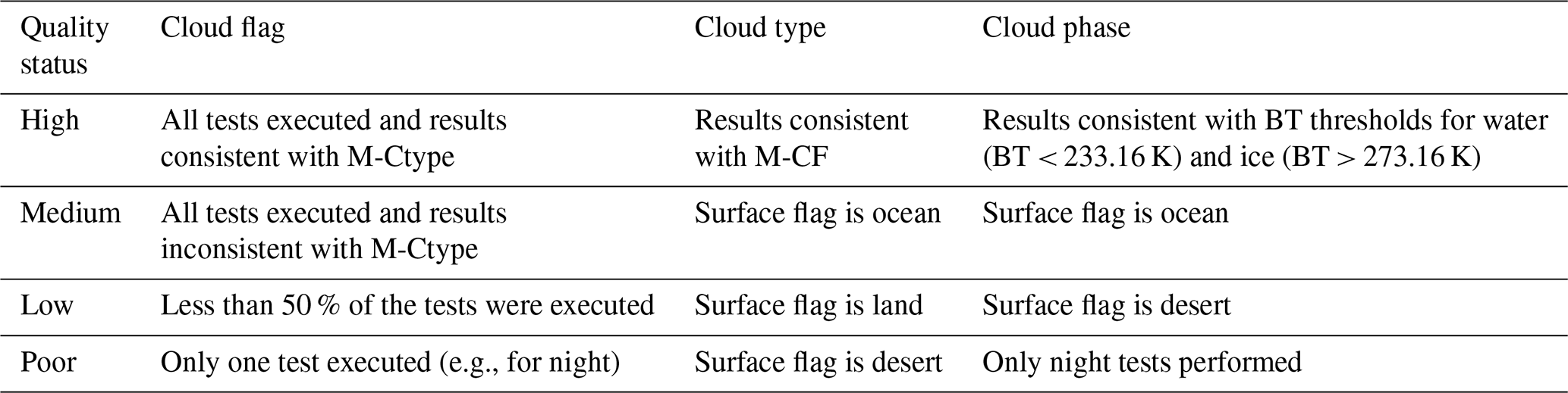
The results of the M-CF and M-Ctype are also combined to a final cloud mask quality flag. A high-quality flag means that both results are consistent.
The algorithm performance and processing chaining has been tested by applying the M-CM processor to scenes from the MODIS and MSG SEVIRI instruments and atmospheric test scenes created synthetically with the EarthCARE end-to-end simulator (Donovan et al., 2023).
3.1 Verification against synthetic test scenes
Three specific synthetic test scenes have been created based on forecasts from the Global Environmental Multiscale (GEM) model (Qu et al., 2022) to test the full chain of EarthCARE processors (Donovan et al., 2023). These test scenes cover a variety of atmospheric situations over ocean, land and ice surface during day- and nighttime. The natural-color RGB images of the three test scenes are provided in Appendix A.
It seems very appealing to verify our cloud algorithm against the test scenes; however, the results should be handled with care because they strongly depend on the assumptions made in the model. But since no observational EarthCARE-like dataset exists, the synthetic model dataset provides the best available proxy for testing the EarthCARE processing chain and synergistic products (Donovan et al., 2023). The most prominent one is the Halifax scene covering a 6000 km long frame starting over Greenland, crossing the eastern end of Canada and ending in the Caribbean (Fig. 5). The scene starts over the Greenland ice sheet with mixed-phase clouds at nighttime, transitioning from deeper clouds with tops up to 6 km around 65∘ N to mixed-phase clouds with tops around 3 km at temperatures as cold as −30 ∘C over the eastern edge of Canada. Below there is a high ice cloud regime followed by a low-level cumulus cloud regime embedded in a marine aerosol layer below an elevated dirty dust layer around 5 km altitude. The original model outputs are generated for 7 December 2015 using the Canadian GEM model (Qu et al., 2022). While the binary cloud flag and cloud phase product provide results for the high-latitude part of the Halifax scene, the cloud type product does not show results there. This is due to the nighttime conditions. The maximum-likelihood classifier also requires information in the visible bands, which makes it impossible to classify cloud types during nighttime. For the cloud flag, only brightness temperature tests have been applied. For this reason, the cloud mask quality flag indicates only poor quality there.
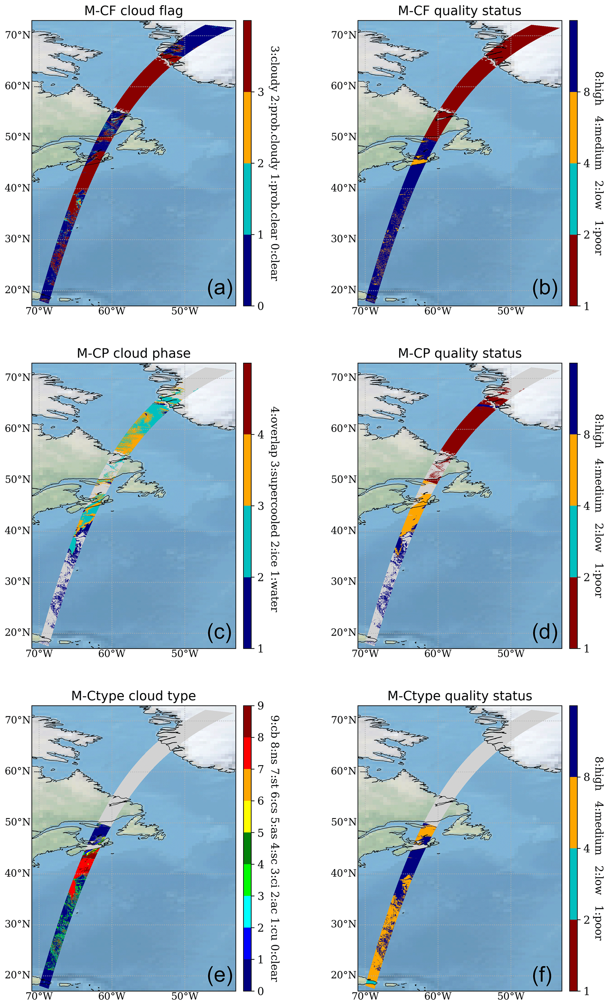
Figure 5M-CM processor applied to the Halifax scene including the binary cloud flag (M-CF) and cloud mask quality flag (a, b), the cloud phase (M-CP) and quality flag (c, d), and cloud types (M-Ctype) and quality flag (e, f). The light-grey-shaded region indicates pixels, labeled as undefined by the processor. cu: cumulus, ac: altocumulus, ci: cirrus, sc: stratocumulus, as: altostratus, cs: cirrostratus, st: stratus, ns: nimbostratus, cb: cumulonimbus.
Verification of the M-CF cloud flag with 3D model input fields
The M-CF cloud flag is verified against the input from the 3D model fields (Donovan et al., 2023). The model cloud flag is calculated based on the extinction profiles at 680 nm from the model input, which we consider the reference. In the first step, we have calculated the cloud optical thickness (COT) as the extinction of radiation along the path from the Earth's surface to the top of atmosphere at 680 nm. The second step defines a certain profile as cloudy applying three different thresholds, COT ≥0.01, COT ≥0.1 and COT ≥1. Figure 6 shows the reference cloud flag, based on the 3D extinction profiles for three different thresholds applied to the COT. When assuming pixels with COT ≥0.01 to be cloudy, the overall cloud fraction of the scene would be 72 %. The cloud fraction decreases to 61 % for COT ≥0.1 and to 37 % for COT ≥1. This demonstrates that the reference cloud mask is very sensitive to the choice of the COT threshold. Using M-CF, a cloud fraction of 50 % is determined for this scene (see Fig. 7). The best agreement between the cloud fraction of the reference cloud flag and the M-CF cloud flag is achieved when applying a threshold of COT ≥0.1. The cloud detection sensitivity of the M-CF algorithm is clearly better than COT ≥1, but in contrast to COT ≥0.1, a few cloudy pixels with probably optically thin clouds are not detected by the M-CF cloud flag. Figure 7 illustrates the performance of the M-CF cloud flag compared to the reference cloud flag (using a threshold of COT ≥0.1) by showing the results of the confusion matrix (e.g., true positive, true negative, false positive, false negative). Both cloud flags are in good agreement for most parts of the scene. Only a few false-cloudy pixels are visible over the ocean, which are most likely thin clouds with COT ≤0.1 that are detected by MSI but not in the cloud flag for COT ≥0.1. The orange pixels in the center of the scene show pixels that are detected as clear-sky by M-CF, while the reference cloud flag defines them as cloudy. This can be explained by the fact that different thresholds are applied for snow and land surface types, but there are inconsistencies between the surface types in the M-CF algorithm and the model data. The M-CF algorithm uses surface information from the X-MET data as input, while the model data use slightly different surface specifications. The scattered false-clear pixels in the lower part of the scene are due to edge pixels of low-level clouds, which are not detected by the M-CF cloud flag.
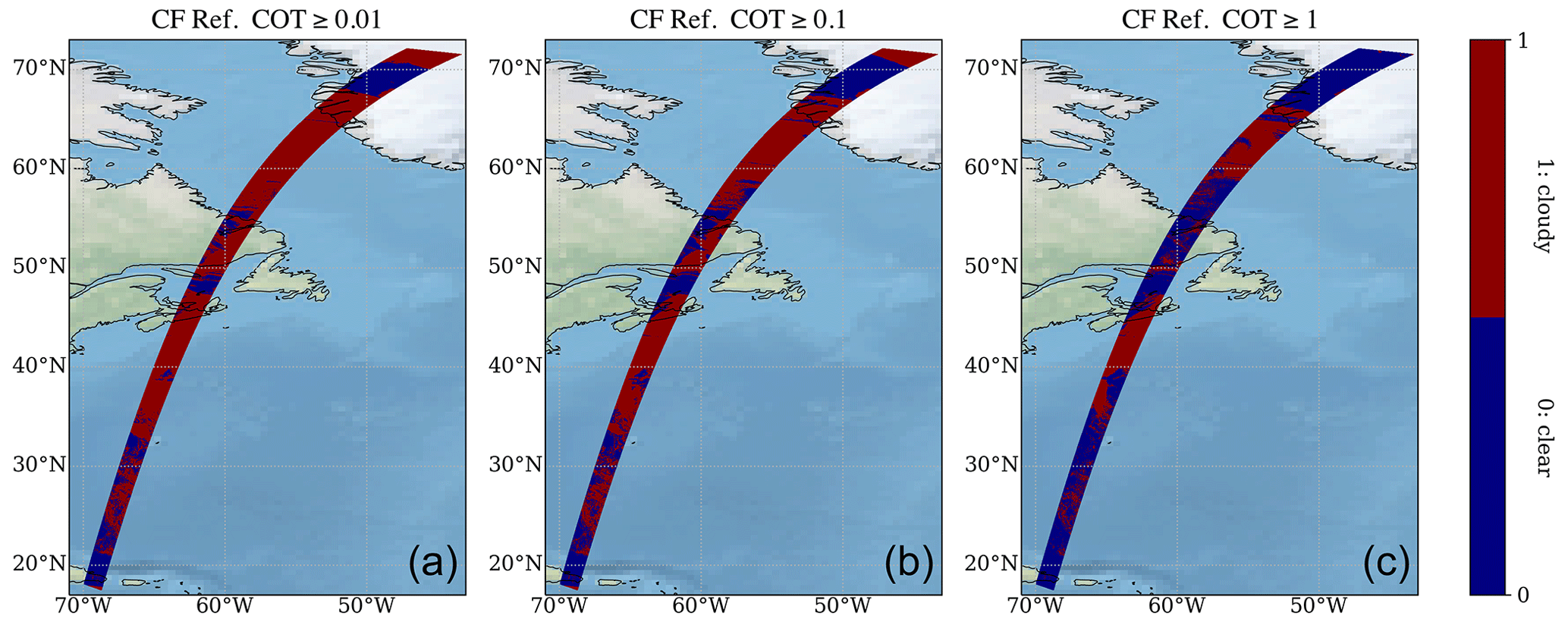
Figure 6Reference cloud flag based on the 3D extinction fields at 680 nm for the Halifax scene. Cloud-free and cloudy areas are identified by applying three different thresholds on the column-integrated cloud optical thickness, COT ≥0.01 (a), COT ≥0.1 (b) and COT ≥1 (c). The resulting cloud fraction is 72 % (COT ≥0.01), 61 % (COT ≥0.1) and 37 % (COT ≥1).
3.2 Verification against MODIS
The M-CM cloud mask algorithm has also been verified against MODIS scenes. In contrast to the synthetic scenes, the MODIS scenes do not rely on the assumptions made in the background model. We have used the calibrated radiances of MODIS Terra Level 1B (L1B) (MOD021KM) of seven similar channels to MSI and global forecast data from the Copernicus Atmosphere Monitoring Service (CAMS) as input for the M-CLD processor. For verification of our results, however, we use the standard MODIS Level 2 (L2) cloud product which makes use of more spectral channels compared to MSI.
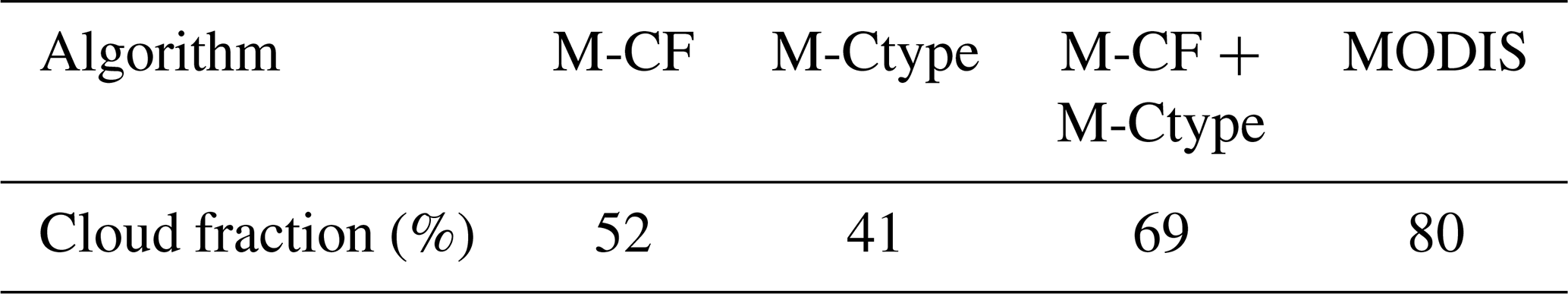
Figure 8 shows the MSI M-CM cloud flag and the MODIS cloud flag for an example over western Africa on 11 September 2021 at 11:50 UTC. Both cloud flags discriminate between clear-sky, cloudy, probably cloudy and probably clear. The false-color RGB image uses the MODIS band 1 (620–670 nm), band 4 (545–565 nm) and band 3 (459–479 nm). The MSI surface flag separates between water (1), land (2), desert (3), vegetation (4), snow (5, 6), sea ice (7), sunglint (8) and undefined (0); the scene over western Africa has no snow or sea ice pixels. Both desert and sunglint represent difficulties for cloud-masking algorithms, which is why the largest differences between the MODIS and MSI cloud flag are found over these surface types. The MSI cloud flag yields a cloud fraction of 52 %, while MODIS results in 80 %. Converting the M-Ctype cloud classes in a binary cloud class results in a cloud fraction of 41 %. The product is independent from M-CF because it uses a maximum-likelihood classifier. When combining both binary M-CM cloud flags into one, the cloud fraction increases to 69 % (Table 2). This result demonstrates that the combination of both independent M-CM cloud products leads to a better agreement with MODIS than just using one of them. The MSI algorithm misses large parts of clouds over desert, but there are also clear differences over the ocean in the upper part of the scenes. These differences are expected because the MODIS cloud tests are based on much more spectral channels. For the majority of clouds, which are visible on the RGB image, the agreement between the MODIS and MSI cloud flag is very good.
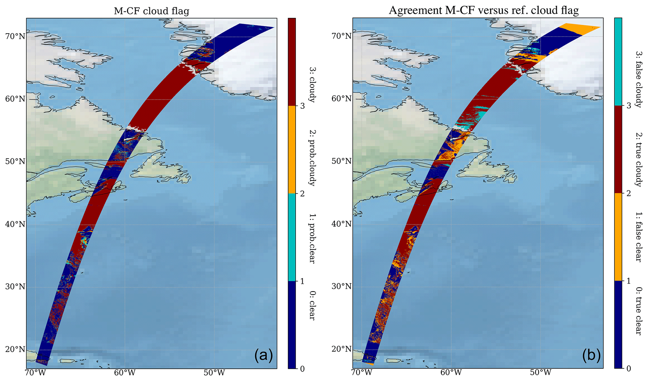
Figure 7M-CF cloud flag (a) and confusion matrix (b) indicating the classification performance (e.g., true cloudy, true clear, false cloudy, false clear) of the binary M-CF and the reference cloud flag (using a threshold of COT ≥0.1). The M-CF cloud fraction is 50 %, while the reference cloud flag results in a cloud fraction of 61 %.
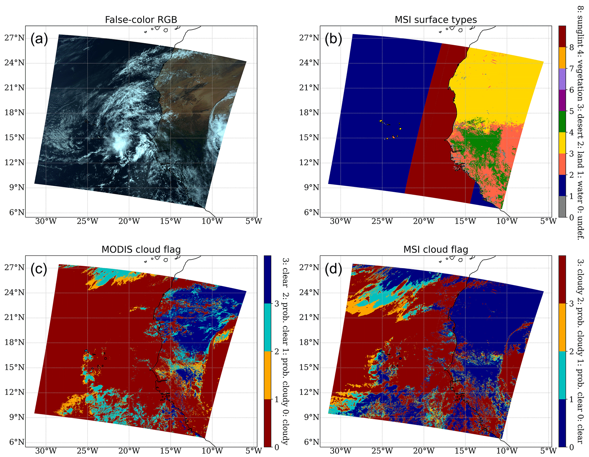
Figure 8M-CM algorithm applied to satellite data from MODIS over western Africa on 11 September 2021 at 11:50 UTC. The MODIS false-color RGB composite (using MODIS bands 1, 4 and 3) is shown in panel (a), the MSI surface flag is shown in panel (b), the MODIS cloud flag is shown in panel (c) and the MSI cloud flag is shown in panel (d). The MSI surface types 5, 6 and 7 are snow and sea ice flags, which are not present in the present case study. While 1 (water), 2 (land), 3 (desert) and 8 (sunglint) are inputs for the processor, type 4 (vegetation) is based on the NDVI and only calculated for clear-sky pixels in the M-CF flag.
Table 2Comparison of the scene cloud fraction between M-CF, M-Ctype, the combination of M-CF and M-Ctype, and MODIS.
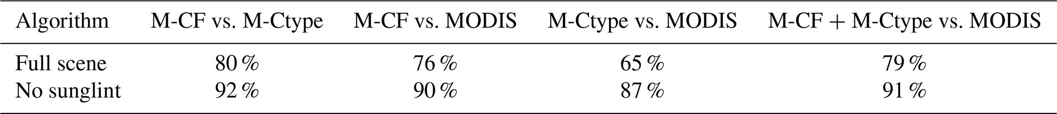
To get more robust statistics, the cloud mask comparison has been done for the full month of September 2021. The MSI cloud flag systematically shows a lower cloud fraction than the MODIS cloud flag. Only in cases with a strong sunglint effect, do the combined M-CF and M-Ctype cloud mask show a higher cloud fraction than MODIS. For assessing the overall agreement between the MSI and MODIS cloud mask, we have calculated the percentage of consistency for both clear-sky and cloudy for all 45 MODIS scenes in September 2021. The results are shown in Table 3. We have intercompared the M-CF vs. M-Ctype products, M-CF vs. MODIS, M-Ctype vs. MODIS and M-CF combined with M-Ctype vs. MODIS. The overall agreement between M-CF and MODIS is 76 %. This results increase to 79 % when combining M-CF and M-Ctype (Table 3). When excluding all pixels that are labeled as sunglint by the M-CM surface flag, the agreement increases to 91 %. This finding demonstrates that large parts of the discrepancies are due to differences in the handling of the algorithms in scenes effected by sunglint, which will be further investigated by tuning the thresholds with real measurements.
Table 3Comparison of the two M-CM cloud flags and the MODIS cloud flag. The agreement in percent is calculated for a binary cloud flag only, where confidently cloudy and probably cloudy is merged to cloudy and the same is done for clear-sky. For M-Ctype, cloud types 1–9 are considered cloudy.
3.3 Verification against MSG SEVIRI
The M-CM cloud mask was also part of a cloud retrieval intercomparison study in the framework of the International Cloud Working Group (ICWG). The ICWG supports the assessment of cloud retrievals applied to passive imagers on board geostationary satellites (Hamann et al., 2014; Wu et al., 2017). Therefore, the M-CM algorithm has been applied to images from the SEVIRI instrument on board Meteosat Second Generation (MSG). As in the comparison with MODIS, SEVIRI also provides similar channel characteristics like the MSI. Nevertheless, one should be aware that this leads to uncertainties through the adaptation to SEVIRI due to differences in the central wavelength and spectral response function, radiative transfer simulations, and generated lookup tables.
Different scientific institutions (e.g., EUMETSAT central facility, European Organisation for the Exploitation of Meteorological Satellites; NWC SAF, Nowcasting Satellite Application Facility; and CM SAF, Climate Monitoring Satellite Application Facility) provided cloud mask data for the SEVIRI disk for the intercomparison study. The individual input data have been transformed into a binary cloud mask separating between cloudy and cloud-free. The M-CM cloud mask was with a cloud fraction of 52 % in the range of the other results ranging from 31 % to 64 %. Figure 9 shows the discrepancies of the different cloud masks results. A pixel value of 0 means that all algorithms are in agreement that it is cloudy. Grey values indicate that all algorithms consistently label the pixel as clear-sky. A disagreement value of 1 shows that half of the algorithms classified a pixel as cloudy, and the other half did so as cloud-free. The main discrepancies between the different cloud masks are found to be over northern Africa, caused by different detection thresholds for thin cirrus clouds over bright surface like desert in this case. It could also be biomass burning aerosol that is classified as clouds by some algorithms. Another area of disagreements is the southern part of the Arabian Peninsula and the adjacent sea.
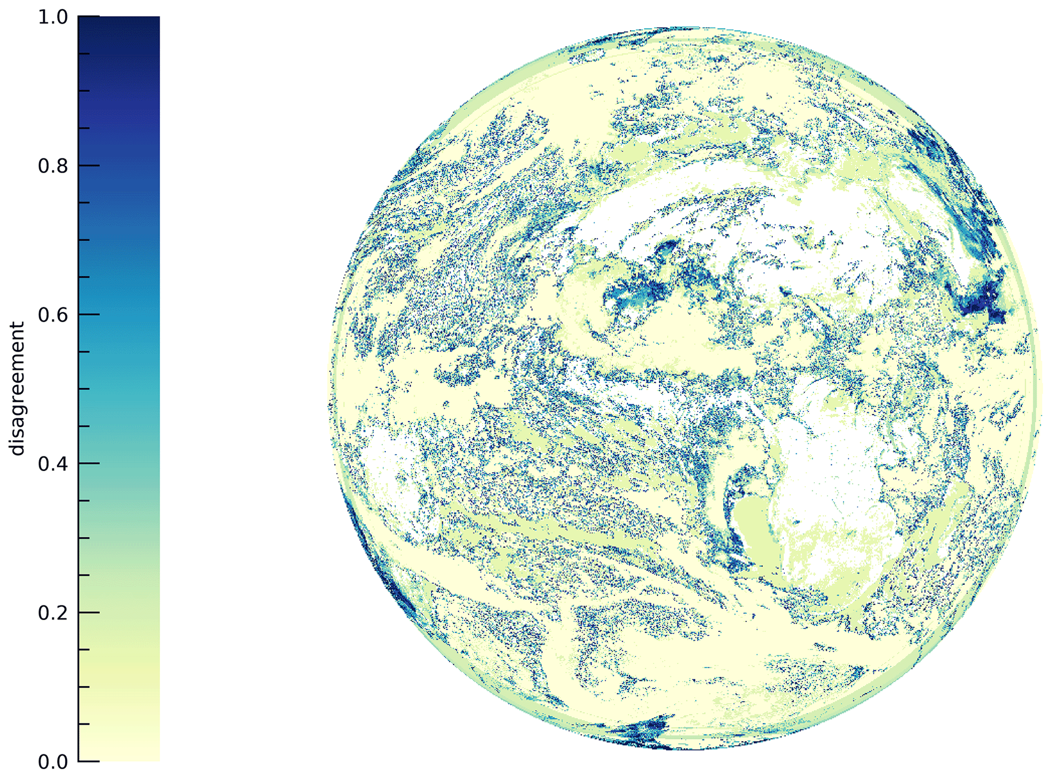
Figure 9Differences between the cloud masks of 12 algorithms for the MSG SEVIRI disk on 13 April 2008. A value of 0 means that all algorithms for this particular pixel set it as cloudy. The grey values mean that all algorithms agree this pixel is cloud-free. In total the disagreement measure is normalized to 1 if the half of the algorithms classify a pixel as cloudy and the other half classify it as cloud-free.
In this paper, the algorithms used by the cloud mask processor (M-CM) for the MSI on board EarthCARE are described. The algorithms provide the cloud flag (M-CF), cloud phase (M-CP) and cloud type (M-Ctype) products. The cloud flag and cloud phase at the cloud top are based on spectral threshold tests for the visible and infrared channels, while the cloud type product is based on a maximum-likelihood classifier. While the cloud type product is only available during daytime, the cloud flag and cloud phase products are also retrieved during nighttime, although with a reduced number of tests (Fig. 1). The M-CM products are an important input for the subsequent retrieval of the cloud optical and physical products (M-COP) (Hünerbein et al., 2023) and the aerosol optical properties (M-AOT) (Docter et al., 2023).
In order to test the algorithm performance and to get a better impression of the products before the EarthCARE launch, the M-CM algorithm has been verified in this study against synthetic test scenes from the EarthCARE end-to-end simulator and satellite data from MODIS and MSG SEVIRI.
Using synthetic test data, it is found that the M-CM products are in good agreement with the products from other processors within the EarthCARE instrument suite and with the 3D model fields used as input to the simulator which can thus be considered the truth. One should keep in mind that in contrast to ATLID or CPR, which provide vertical profile information, MSI is a passive instrument that retrieves cloud properties at the cloud top or, for aerosol and optically thin clouds, total column-integrated information. The synergistic products using data from MSI and ATLID will help to better understand some of the uncertainties in the MSI products (Haarig et al., 2023).
An overall agreement of 79 % was found between the MSI and the MODIS cloud flag using 1 month of MODIS data over Cabo Verde in September 2021. The agreement significantly improves to 91 % when excluding the sunglint areas from the comparison. Ocean areas characterized by sunglint represent some of the most challenging scenes for cloud-masking algorithms. This indicates that further adjustments are needed for the thresholds of the M-CM cloud flag for sunglint conditions to improve the performance. However, the MSI images are less affected by sunglint in comparison to MODIS due to the fact that the MSI is tilted sideways, with 35 km of the full 150 km swath on the sun-facing side and 115 km on the other side of the nadir track.
The M-CM algorithm has also been applied to measurements from MSG SEVIRI, and the results have been compared against other cloud mask algorithms in the frame of the International Cloud Working Group. The comparison has demonstrated that the M-CM performance lies in the range of the other cloud masks.
Planned improvements in M-CM will include dynamic thresholds for the threshold tests for the cloud flag. We propose that this tuning should be done after launch once real observations will be available. A tuning of the M-CM thresholds towards better agreement with MODIS is not optimal in the current state because of the spectral differences between MSI and MODIS. While MSI features 7 spectral bands, MODIS has 36 spectral bands, allowing for better cloud detection performance. The advantage of the MSI observations are, in contrast to MODIS, that MSI is flying together with active instruments (e.g., ATLID and CPR) on the same platform, which will allow for unique synergies of cloud products from different instruments.
The algorithm verification in the present study uses synthetic test scenes and data from other satellite platforms as the basis. During the validation phase after the EarthCARE launch, dedicated campaigns will be conducted using ground-based and airborne instruments, which will offer the opportunity for a more comprehensive validation of the MSI cloud products. Also geostationary satellites will be used for the validation to support the selection of suitable validation datasets and to provide complementary reference datasets on a global scale. Meteosat Third Generation (MTG) was launched in 2022 into geostationary orbit (Holmlund et al., 2021), offering with its Flexible Combined Imager (FCI) with 16 spectral channels and up to 500 m spatial sampling excellent opportunities for the validation of and synergies with the MSI products.
Further improvements in the M-CM product are expected once real observations are available due to its flexible design based on configuration files, which allows for easy adjustment, e.g., of cloud mask thresholds without modifying the source code of the whole algorithm chain.
In contrast to the pre-launch MSI test data presented in this study, the MSI spectral bands are affected by a shift in the central wavelength depending on the instrument viewing angle. This effect is caused due to imperfections in the bandpass filters on the curved optical lenses (e.g., Wehr et al., 2023; Wang et al., 2022). Investigations are ongoing to mitigate this effect in the Level 2 M-CLD and M-AOT retrievals. During the validation phase, aircraft measurements with high spectral resolution will further help to quantify the impact of the central wavelength shift on the MSI cloud and aerosol products.
For the three test scenes natural-color RGB images are generated to visualize several types of atmospheric and surface features. The natural-color RGB is composed of the VIS, NIR and SWIR-1 channel data. The images have been linearly stretched within the reflectance ranges to the full range of display values from 0–255 bytes to improve the contrast.
The benefit is the easy interpretation because most of the colors of the image are very similar to a true-color image of the Earth. Figure A1 shows the RGB images for the three test scenes, which includes clouds, snow, vegetation, sunglint and clear skies. Snow on the ground as well as ice over mountains, frozen lakes and sea ice appear cyan in the RGB images (Fig. A1b). The more homogeneous the snow/ice cover is, the brighter the cyan color will be. Snow and ice on mountains will therefore be depicted in a stronger cyan color than snowy surfaces on ground, which are often disrupted by vegetation. In addition, clouds with ice crystals also appear cyan in the RGB images (Fig. A1a) as the ice crystals reflected at 0.67 and 0.865 µm and absorb solar radiation at 1.65 µm. Further different cloud heights, ice crystal habits and sun zenith angles lead to an inhomogeneous color pattern. The ocean and lakes in the RGB images appear in dark black (Fig. A1c). Vegetation is indicated by green colors because of the stronger reflection of solar radiation at 0.865 µm than at 0.67 µm (Fig. A1a, e.g., Caribbean island in the Halifax scene). For detailed information on how to interpret RGB images, see the RGB color guide (Eumetrain, 2022).
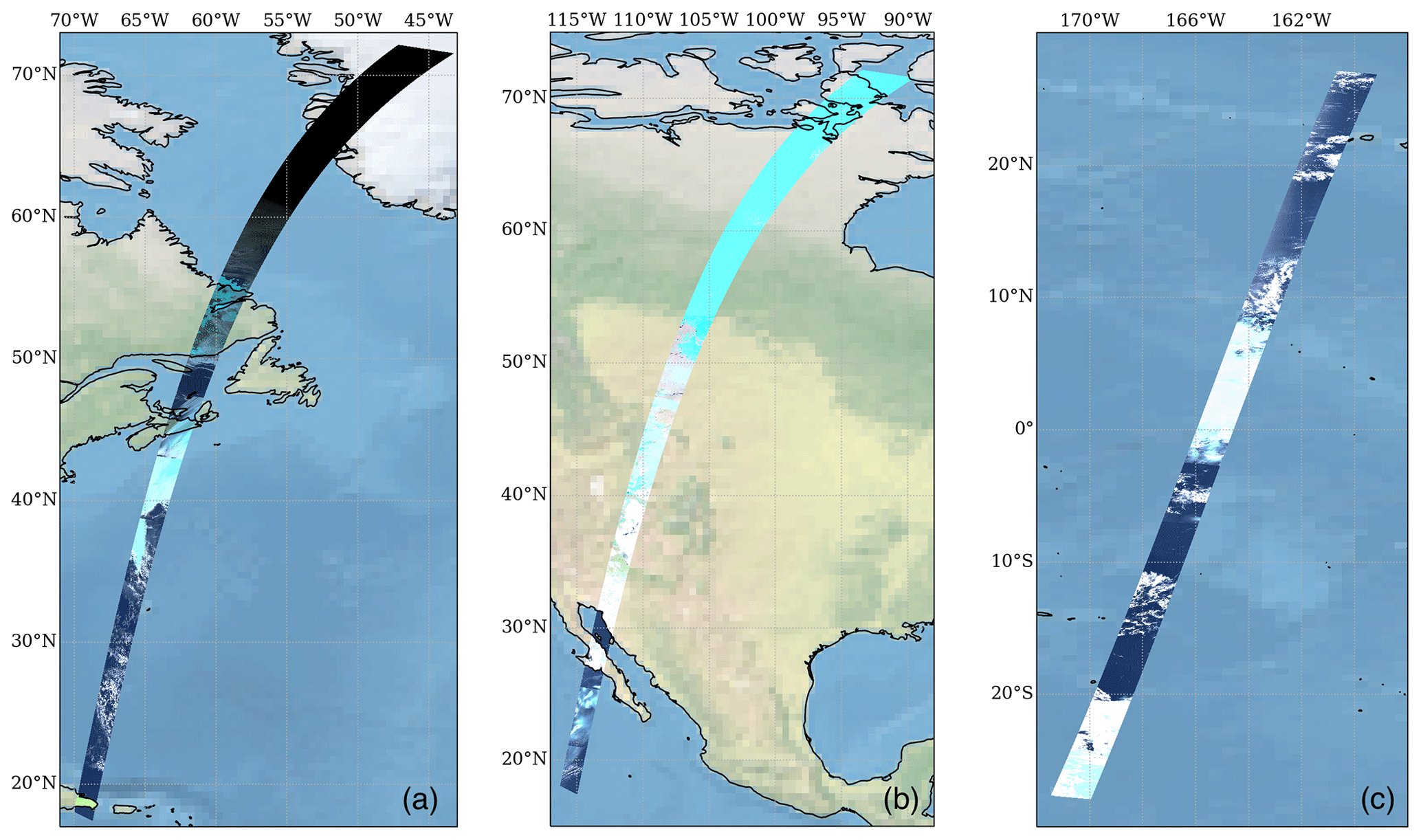
Figure A1Natural-color RGB images generated from the MSI VIS, NIR and SWIR-1 channels for (a) Halifax, (b) Baja and (c) Hawaii (Donovan et al., 2023).
The EarthCARE Level 2 demonstration products from simulated scenes, including the MSI cloud mask products discussed in this paper, are available at https://doi.org/10.5281/zenodo.7117115 (van Zadelhoff et al., 2022).
The manuscript was prepared by AH, SB and HD. The M-CM code was developed by AH and SH. AW generated the dataset and created the plots for the ICWG results.
The contact author has declared that none of the authors has any competing interests.
Publisher’s note: Copernicus Publications remains neutral with regard to jurisdictional claims in published maps and institutional affiliations.
This article is part of the special issue “EarthCARE Level 2 algorithms and data products”. It is not associated with a conference.
The authors thank Tobias Wehr and Michael Eisinger for their continuous support over many years and the EarthCARE developer team for valuable discussions during various meetings. The authors would like to express their gratitude to the MODIS and SEVIRI science team for providing their data to the scientific community. The authors acknowledge ESA for the financial support.
This research has been funded by the European Space Agency (ESA) (grant nos. 4000112018/14/NL/CT (APRIL) and 4000134661/21/NL/AD (CARDINAL)).
The publication of this article was funded by the Open Access Fund of the Leibniz Association.
This paper was edited by Robin Hogan and reviewed by two anonymous referees.
Ackerman, A., Strabala, K., Menzel, P., Frey, R., Moeller, C., Gumley, L., Baum, B., Seemann, S., and Zhang, H.: Discriminating Clear-Sky from Cloud with MODIS—Algorithm Theoretical Basis Document (MOD35), ATBD Reference Number: ATBD-MOD-06, Goddard Space Flight Center, https://atmosphere-imager.gsfc.nasa.gov/sites/default/files/ModAtmo/MOD35_ATBD_Collection6_1.pdf (last access: 31 May 2023), 2002. a, b
Ackerman, S. A., Strabala, K. I., Menzel, W. P., Frey, R. A., Moeller, C. C., and Gumley, L. E.: Discriminating clear sky from clouds with MODIS, J. Geophys. Res.-Atmos., 103, 32141–32157, https://doi.org/10.1029/1998JD200032, 1998. a
Docter, N., Preusker, R., Filipitsch, F., Kritten, L., Schmidt, F., and Fischer, J.: Aerosol optical depth retrieval from the EarthCARE multi-spectral imager: the M-AOT product, EGUsphere [preprint], https://doi.org/10.5194/egusphere-2023-150, 2023. a
Donovan, D. P., Kollias, P., Velázquez Blázquez, A., and van Zadelhoff, G.-J.: The Generation of EarthCARE L1 Test Data sets Using Atmospheric Model Data Sets, EGUsphere [preprint], https://doi.org/10.5194/egusphere-2023-384, 2023. a, b, c, d, e, f
Eisinger, M., Wehr, T., Kubota, T., Bernaerts, D., and Wallace, K.: The EarthCARE production model and auxiliary products, Atmos. Meas. Tech., in preparation, 2023. a, b
Eumetrain: RGB color guide, https://www.eumetrain.org/index.php/rgb-color-guide (last access: 22 November 2022), 2022. a
Haarig, M., Hünerbein, A., Wandinger, U., Docter, N., Bley, S., Donovan, D., and van Zadelhoff, G.-J.: Cloud top heights and aerosol columnar properties from combined EarthCARE lidar and imager observations: the AM-CTH and AM-ACD products, EGUsphere [preprint], https://doi.org/10.5194/egusphere-2023-327, 2023. a
Hamann, U., Walther, A., Baum, B., Bennartz, R., Bugliaro, L., Derrien, M., Francis, P. N., Heidinger, A., Joro, S., Kniffka, A., Le Gléau, H., Lockhoff, M., Lutz, H.-J., Meirink, J. F., Minnis, P., Palikonda, R., Roebeling, R., Thoss, A., Platnick, S., Watts, P., and Wind, G.: Remote sensing of cloud top pressure/height from SEVIRI: analysis of ten current retrieval algorithms, Atmos. Meas. Tech., 7, 2839–2867, https://doi.org/10.5194/amt-7-2839-2014, 2014. a
Hollstein, A., Fischer, J., Carbajal Henken, C., and Preusker, R.: Bayesian cloud detection for MERIS, AATSR, and their combination, Atmos. Meas. Tech., 8, 1757–1771, https://doi.org/10.5194/amt-8-1757-2015, 2015. a
Holmlund, K., Grandell, J., Schmetz, J., Stuhlmann, R., Bojkov, B., Munro, R., Lekouara, M., Coppens, D., Viticchie, B., August, T., Theodore, B., Watts, P., Dobber, M., Fowler, G., Bojinski, S., Schmid, A., Salonen, K., Tjemkes, S., Aminou, D., and Blythe, P.: Meteosat Third Generation (MTG): Continuation and Innovation of Observations from Geostationary Orbit, B. Am. Meteorol. Soc., 102, E990–E1015, https://doi.org/10.1175/BAMS-D-19-0304.1, 2021. a
Hughes, M. J. and Kennedy, R.: High-quality cloud masking of Landsat 8 imagery using convolutional neural networks, Remote Sens., 11, 2591, https://doi.org/10.3390/rs11212591, 2019. a
Hünerbein, A., Bley, S., Deneke, H., Meirink, J. F., van Zadelhoff, G.-J., and Walther, A.: Cloud optical and physical properties retrieval from EarthCARE multi-spectral imager: the M-COP products, EGUsphere [preprint], https://doi.org/10.5194/egusphere-2023-305, 2023. a, b
Illingworth, A. J., Barker, H., Beljaars, A., Ceccaldi, M., Chepfer, H., Clerbaux, N., Cole, J., Delanoë, J., Domenech, C., Donovan, D. P., Fukuda, S., Hirakata, M., Hogan, R. J., Huenerbein, A., Kollias, P., Kubota, T., Nakajima, T., Nakajima, T. Y., Nishizawa, T., Ohno, Y., Okamoto, H., Oki, R., Sato, K., Satoh, M., Shephard, M. W., Velázquez-Blázquez, A., Wandinger, U., Wehr, T., and van Zadelhoff, G.-J.: The EarthCARE satellite: The next step forward in global measurements of clouds, aerosols, precipitation, and radiation, Bulletin of the American Meteorological Society, 96, 1311–1332, 2015. a
IPCC: Climate Change 2021: The Physical Science Basis. Contribution of Working Group I to the Sixth Assessment Report of the Intergovernmental Panel on Climate Change, edited by: Masson-Delmotte, V., Zhai, P., Pirani, A., Connors, S. L., Péan, C., Berger, S., Caud, N., Chen, Y., Goldfarb, L., Gomis, M. I., Huang, M., Leitzell, K., Lonnoy, E., Matthews, J. B. R., Maycock, T. K., Waterfield, T., Yelekçi, O., Yu, R., and Zhou, B., Cambridge University Press, Cambridge, United Kingdom and New York, NY, USA, ISBN: 978-92-9169-158-6, in press, https://www.ipcc.ch/report/ar6/wg1/downloads/report/IPCC_AR6_WGI_SPM_final.pdf (last access: 31 May 2023), 2021. a
Li, Z., Shen, H., Cheng, Q., Liu, Y., You, S., and He, Z.: Deep learning based cloud detection for medium and high resolution remote sensing images of different sensors, ISPRS J. Photogramm., 150, 197–212, https://doi.org/10.1016/j.isprsjprs.2019.02.017, 2019. a
Liu, Y., Key, J. R., Frey, R. A., Ackerman, S. A., and Menzel, W.: Nighttime polar cloud detection with MODIS, Remote Sens. Environ., 92, 181–194, https://doi.org/10.1016/j.rse.2004.06.004, 2004. a
Mateo-García, G., Gómez-Chova, L., and Camps-Valls, G.: Convolutional neural networks for multispectral image cloud masking, in: 2017 IEEE International Geoscience and Remote Sensing Symposium (IGARSS), Fort Worth, TX, USA, 23–28 July 2017, IEEE, 2255–2258, https://doi.org/10.1109/IGARSS.2017.8127438, 2017. a
Nakajima, T. Y., Tsuchiya, T., Ishida, H., Matsui, T. N., and Shimoda, H.: Cloud detection performance of spaceborne visible-to-infrared multispectral imagers, Appl. Optics, 50, 2601, https://doi.org/10.1364/ao.50.002601, 2011. a
Pavolonis, M. J. and Heidinger, A. K.: Daytime cloud overlap detection from AVHRR and VIIRS, J. Appl. Meteorol. Clim., 43, 762–778, 2004. a, b
Pavolonis, M. J., Heidinger, A. K., and Uttal, T.: Daytime global cloud typing from AVHRR and VIIRS: Algorithm description, validation, and comparisons, J. Appl. Meteorol., 44, 804–826, 2005. a, b
Pinty, B. and Verstraete, M.: GEMI: a non-linear index to monitor global vegetation from satellites, Vegetatio, 101, 15–20, https://doi.org/10.1007/BF00031911, 1992. a
Platnick, S., King, M. D., Ackerman, S. A., Menzel, W. P., Baum, B. A., Riedi, J. C., and Frey, R. A.: The MODIS cloud products: Algorithms and examples from Terra, IEEE T. Geosci. Remote, 41, 459–473, 2003. a
Qu, Z., Donovan, D. P., Barker, H. W., Cole, J. N. S., Shephard, M. W., and Huijnen, V.: Numerical Model Generation of Test Frames for Pre-launch Studies of EarthCARE’s Retrieval Algorithms and Data Management System, Atmos. Meas. Tech. Discuss. [preprint], https://doi.org/10.5194/amt-2022-300, in review, 2022. a, b
Rossow, W. B. and Garder, L. C.: Cloud detection using satellite measurements of infrared and visible radiances for ISCCP, J. Climate, 6, 2341–2369, 1993. a, b
Rossow, W. B. and Schiffer, R. A.: Advances in understanding clouds from ISCCP, B. Am. Meteorol. Soc., 80, 2261–2288, https://doi.org/10.1175/1520-0477(1999)080<2261:AIUCFI>2.0.CO;2, 1999. a
Saunders, R. W. and Kriebel, K. T.: An improved method for detecting clear sky and cloudy radiances from AVHRR data, Int. J. Remote Sens., 9, 123–150, 1988. a, b, c
Saunders, R. W., Matricardi, M., and Brunel, P.: An Improved Fast Radiative Transfer Model for Assimilation of Satellite Radiances Observations, Q. J. Roy. Meteor. Soc., 125, 1407–1425, 1999. a
Schiffer, R. A. and Rossow, W. B.: The International Satellite Cloud Climatology Project (ISCCP): The First Project of the World Climate Research Programme, B. Am. Meteorol. Soc., 64, 779–784, https://doi.org/10.1175/1520-0477-64.7.779, 1983. a
Skakun, S., Wevers, J., Brockmann, C., Doxani, G., Aleksandrov, M., Batič, M., Frantz, D., Gascon, F., Gómez-Chova, L., Hagolle, O., López-Puigdollers, D., Louis, J., Lubej, M., Mateo-García, G., OSMAN, J., Peressutti, D., Pflug, B., Puc, J., Richter, R., Roger, J.-C., Scaramuzza, P., Vermote, E., Vesel, N., Zupanc, A., and Žust, L.: CMIX: Cloud Mask Intercomparison eXercise, in: Living Planet Symposium, Bonn, Germany, 23–27 May 2022, https://elib.dlr.de/187698/ (last access: 31 May 2023), 2022. a
Strabala, K. I., Ackerman, S. A., and Menzel, W. P.: Cloud Properties inferred from 8–12-µm Data, J. Appl. Meteorol. Clim., 33, 212–229, 1994. a, b
van Zadelhoff, G.-J., Barker, H. W., Baudrez, E., Bley, S., Clerbaux, N., Cole, J. N. S., de Kloe, J., Docter, N., Domenech, C., Donovan, D. P., Dufresne, J.-L., Eisinger, M., Fischer, J., García-Marañón, R., Haarig, M., Hogan, R. J., Hünerbein, A., Kollias, P., Koopman, R., Madenach, N., Mason, S. L., Preusker, R., Puigdomènech Treserras, B., Qu, Z., Ruiz-Saldaña, M., Shephard, M., Velázquez-Blazquez, A., Villefranque, N., Wandinger, U., Wang, P., and Wehr, T.: EarthCARE level-2 demonstration products from simulated scenes, Zenodo [data set], https://doi.org/10.5281/zenodo.7117116, 2022. a
Wang, M., Nakajima, T. Y., Roh, W., Satoh, M., Suzuki, K., Kubota, T., and Yoshida, M.: Evaluation of the smile effect on the Earth Clouds, Aerosols and Radiation Explorer (EarthCARE)/Multi-Spectral Imager (MSI) cloud product, EGUsphere [preprint], https://doi.org/10.5194/egusphere-2022-736, 2022. a
Wehr, T., Kubota, T., Tzeremes, G., Wallace, K., Nakatsuka, H., Ohno, Y., Koopman, R., Rusli, S., Kikuchi, M., Eisinger, M., Tanaka, T., Taga, M., Deghaye, P., Tomita, E., and Bernaerts, D.: The EarthCARE Mission – Science and System Overview, EGUsphere [preprint], https://doi.org/10.5194/egusphere-2022-1476, 2023. a, b
Wu, D. L., Baum, B. A., Choi, Y.-S., Foster, M. J., Karlsson, K.-G., Heidinger, A., Poulsen, C., Pavolonis, M., Riedi, J., Roebeling, R., Sherwood, S., Thoss, A., and Watts, P.: Toward Global Harmonization of Derived Cloud Products, B. Am. Meteorol. Soc., 98, ES49–ES52, https://doi.org/10.1175/BAMS-D-16-0234.1, 2017. a
Zekoll, V., Main-Knorn, M., Alonso, K., Louis, J., Frantz, D., Richter, R., and Pflug, B.: Comparison of Masking Algorithms for Sentinel-2 Imagery, Remote Sens., 13, 137, https://doi.org/10.3390/rs13010137, 2021. a
- Abstract
- Introduction
- M-CM algorithm description
- Verification of the M-CM algorithm performance
- Conclusions
- Appendix A: Natural-color RGB images of the synthetic test scenes
- Data availability
- Author contributions
- Competing interests
- Disclaimer
- Special issue statement
- Acknowledgements
- Financial support
- Review statement
- References