Estimation of extreme precipitation events in Estonia and Italy using dual-polarization weather radar quantitative precipitation estimations

Evaluating extreme rainfall for a certain location is commonly considered when designing stormwater management systems. Rain gauge data are widely used to estimate rainfall intensities for a given return period. However, the poor spatial and temporal resolution of operational gauges is the main limiting factor. Several studies have used rainfall estimates based on weather radar horizontal reflectivity (Z_h), but they come with a great caveat: while proven reliable for low or moderate rainfall rates, they are subject to major errors in extreme rainfall and convective cases. It is widely known that C-band weather radar can underestimate precipitation intensity due to signal attenuation or overestimate it due to hail and clutter contamination. From the late 1990s, dual-polarization weather radar started to become operational in the national surveillance radar network in Europe, providing innovative quantitative precipitation estimation (QPE) based on polarimetric variables. This study circumvents Z_h shortcomings by using specific differential-phase (K_dp) data from operational dual-polarization C-band weather radars. The rain intensity estimates based on a specific differential-phase data are immune to attenuation and less affected by hail contamination.

In this study, for the first time, QPEs based on polarimetric observations by operational C-band weather radars and without any rain gauge adjustments are analyzed. The purpose is to estimate return periods for 1 h rainfall total computed from polarimetric weather radar data using non-adjusted QPEs based on R(Z_h,K_dp) data and to compare the results with those derived using R(Z_h) and rain gauge data. Only the warm period during the year is considered here, as most of the extreme precipitation events for such a duration occur for both places studied (Italy and Estonia) at this time. Limiting the dataset to warm periods also allows us to use the radar-based rainfall quantitative precipitation estimations, which are more reliable than the snowfall ones. Data from operational dual polarimetric C-band weather radar sites are used from both Italy and Estonia. Given climatologically homogeneous regions, this study demonstrates that polarimetric weather radar observations can provide reliable QPEs compared to single-polarization estimates with respect to rain gauges and that they can provide a reliable estimation of return periods of 1 h rainfall total, even for relatively short time series.

1 Introduction

The increase in impervious surfaces due to urbanization leads to an increase in flooding frequency due to poor infiltration and faster concentration times. Hydrological changes, driven by heavy urbanization, and resulting impacts on extreme rainfall are also being established: a significant amount of research over the last 20 years has shown a strong relationship between urban areas and local microclimates.

The Intergovernmental Panel on Climate Change (IPCC) Sixth Assessment Report (IPCC, 2021) increased interest in short-duration rainfall extreme estimations as several Earth regions are likely to be affected by an increase in heavy-precipitation events in the near future due to global warming. In Europe, van den Besselaar et al. (2012) demonstrated that higher latitudes are still experiencing an incremental increase in intensity and frequency of extreme events and correspondingly in heavy-precipitation events. For all these reasons, studies on extreme annual rainfall maximum depths for short durations are extremely relevant for hydrological studies, water management, and urban-area development (Marra et al., 2017).

However, the reliability of traditional rainfall depth estimations is often limited by the low spatial density of rain gauge networks, particularly for short durations (Overeem et al., 2010). Nevertheless, single-polarization weather radars can provide quantitative precipitation estimations (QPEs), based on empirical relationships between the equivalent reflectivity factor at horizontal polarization (Z_h) and the rain rate with proper spatial and temporal resolution. Several studies have investigated statistics of extreme areal rainfall depths obtained from single-polarization weather radar (Frederick et al., 1977; Allen and De Gaetano, 2005; Overeem et al., 2008, 2009a, b, 2010; Marra and Morin, 2015; Panziera et al., 2018; Marra et al., 2022). Keupp et al. (2017) and Fabry et al. (2017) offer a complete review of monthly or annual rainfall climatology based on weather radar observations in Europe and the contiguous United States (CONUS) area, respectively.

However, due to signal attenuation at the C-band (Delrieu et al., 2000) and due to hail contamination (Ryzhkov et al., 2013), the horizontal radar reflectivity (Z_h) is subject to significant errors, especially during intense rainfall and convective-precipitation events. As stated by Fairman et al. (2015), relevant QPE underestimations typically occur in mountainous areas and far away from the weather radar; beam blocking and overshooting also cause large differences between radar-based QPEs and reference gauges. To overcome these limitations, several adjustment techniques have been developed that correct QPEs, derived from single-polarization weather radar, with rain gauge measurements (Einfalt and Michaelides, 2008; Goudenhoofdt and Delobbe, 2009). Overeem et al. (2009b) derived short-duration extreme rainfall depths from gauge-adjusted weather radar QPEs. Barndes et al. (2001), Ryzhkov et al. (2005), and Vulpiani et al. (2012) demonstrated that polarimetric rainfall estimation algorithms based on specific differential phase (K_dp) outperform the conventional QPEs based on horizontal radar reflectivity, being immune from partial beam blocking, attenuation, hail contamination, and weather radar miscalibration. Several studies have focused on the evaluation of R(K_dp) relationship performances with respect to traditional R(Z_h) for precipitation events (Paulitsch et al., 2009; Moisseev et al., 2010; Cremonini and Bechini, 2010). Voormansik et al. (2021a) deeply analyzed 5 years of QPEs derived from operational C-band polarimetric weather radar in Estonia and Italy, demonstrating that blended R(Z_h,K_dp) algorithms provide good-quality QPEs.

For the first time, this study investigates the statistical properties of annual rainfall maxima for 1 h rainfall totals, analyzing QPEs derived from R(Z_h,K_dp) observations by operational dual-polarization C-band weather radars in two different climate regions. The results from short-period weather radar observations are compared with statistics obtained from gauge measurements and QPEs based on traditional horizontal radar reflectivity. Section 2 provides a description of study areas, polarimetric weather radar systems, and algorithms used to derive QPEs. In Sect. 3 extreme-value statistics are applied to fit the theoretical distributions, providing rainfall depth as a function of duration for given return periods. Finally, the Discussion (Sect. 4) and Conclusions (Sect. 5) follow.

2 Materials and methods

This study focuses on QPEs based on polarimetric C-band weather radar, operating in northern Italy and Estonia. The studied period is limited to the warm period of the year as most of the extreme precipitation events at short temporal scales take place at this time. Limiting the dataset to a warm period also helps to exclude weather radar observations that come from snow or ice crystals, a requirement for reliable rainfall intensity estimations based on R(Z_h,K_dp).

2.1 The study areas

​​​​​​​This study focuses on areas in Piedmont, Italy, and Estonia, covered by operational dual-polarization Doppler C-band weather radars operated by the local weather services.

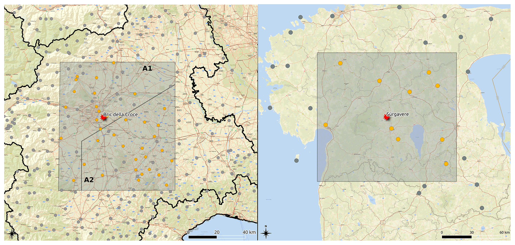
Figure 1 The study areas. On the left the two Italian study areas (EPSG:32632) and on the right the Estonian area (EPSG:3301). The dot symbols show the tipping-bucket rain gauges of the local hydrological networks; orange dot symbols are the tipping-bucket rain gauges used in the study; the red stars are the weather radar locations, the Bric della Croce radar site and Sürgavere radar location, respectively; basemap: Esri, https://basemaps.arcgis.com/arcgis/rest/services/World_Basemap_v2/VectorTileServer (last access: 5 November 2022).

Piedmont is located in northwestern Italy, in the upper areas of the Po Valley; the central part of the region is relatively flat (300–200 m a.s.l.) with the Turin Hill reaching 770 m a.s.l. The Alps surround plains with altitudes ranging from 1000 m to more than 4500 m a.s.l. The two areas considered in this study are centered on the Turin Hill, and they extend for about 30–50 km from the weather radar, corresponding to about 7300 km² altogether (Fig. 1, the left map). To ensure QPE data quality, the choice to restrict the study areas close to the radar site is driven by the following main reasons:

1. to reduce weather radar beam-broadening and beam-propagation effects,

2. to avoid the Alps' complex orography in the western and northern directions,

3. to limit the weather radar beam height above ground,

4. to avoid or to limit spatial non-stationarity of the generalized extreme value (GEV) parameters and their dependence on geomorphology (altitude, terrain slope, and exposition).

The Piedmont rainfall regime is sub-continental with a dry season during winter; the main maximum precipitation occurs during fall, and a secondary maximum occurs during spring–summer (Devoli et al., 2018); convective-precipitation events are very frequent from late spring to early fall. Pavan et al. (2018) reconstructed rainfall climatology over the Po Valley from gauge observations from 1961 to 2015, showing that, despite the relatively small extent of the whole study area, there are different precipitation regimes between the area A1, located close to the Alps (wetter), and the area A2, the flats south of the Turin Hill (drier). It is worth mentioning that the average annual rainfall within each single study area is uniform.

The Bric della Croce weather radar, operated by the Regional Agency for Environment Protection (Arpa Piemonte) is located on the top of the Turin Hill. The operational radar completes fully polarimetric volume scans, made of 11 elevations over an up to 170 km range with 340 m range bin resolution. Quantitative precipitation estimations (QPEs), based on horizontal reflectivity, are extensively described by Cremonini and Tiranti (2018); meanwhile, K_dp-based precipitation estimations are derived according to Wang and Chandrasekar (2009). The closest observations to the weather radar (up to 8 km) have been left out due to heavy ground clutter contamination and unreliable estimations of K_dp. Being focused on convective precipitation, this study limits analysis to the warm season ranging in Italy from April to October. Bric della Croce data range from 2014 to 2020 with 5 min interval time resolution. The data inspection for quality purposes has shown that the annual maxima for the years 2015 and 2016 are unreliable due to frequent weather radar failures during the warm season; for this reason, these years have been excluded from the following analysis.

Arpa Piemonte also operates an automated ground weather network made up of more than 350 rain gauges with 0.2 mm resolution and 300 mm h⁻¹ maximum detectable rainfall intensity; 1 min rainfall observations have been available since 1988. Annual hourly rainfall maxima are derived from gauge observations corrected for underestimations at high rainfall intensities according to Lanza et al. (2010) and Vuerich et al. (2009). Annual hourly rainfall maxima are manually quality-controlled to identify possible mechanical failures and incomplete time series. In this work, 1 min resolution tipping-bucket rain gauges located within the two study areas and running for at least 15 years have been used. Area A1 north and west of the weather radar site contains 27 (24 gauges actually used in the study) gauges, while area A2 contains 25 (23 gauges actually used in the study) gauges; the annual hourly precipitation maxima concern years from 1988 to 2020.

The study area in Estonia is centered on the continental part of the country, and it extends for about 70 km around the radar corresponding to 16 911 km². Estonia is a flat country with a mean elevation of about 50 m a.s.l., and the highest point is 318 m a.s.l in the more hilly southeast (Fig. 1, right map). Estonia has a temperate climate with the heaviest rainfall in late summer. Convective precipitation is common in the area from May to September (Voormansik et al., 2021b). There are distinct differences in the precipitation climate between continental Estonia and the islands in the western part as the latter are much drier (Tammets and Jaagus, 2012). This variance is caused by different thermal regimes of sea and land surfaces. Sub-daily rainfall extremes in the Nordic–Baltic region from rain gauges were analyzed by Olsson et al. (2022). Variations in 1 h return levels in Estonia were found in some of the stations outside of our study area. Generally higher return levels were found in the eastern part of the country and lower return levels in the western part. The 1 h return levels were shown to be nearly uniform in the central part of Estonia without significant variations in the shape parameter (see Sect. 2.1.1), which was close to zero. In the study area, we can thus expect a uniform precipitation regime.

The Sürgavere radar is situated in the northern part of Sakala Upland on top of the Sürgavere Hill (128 m a.s.l.). The Sürgavere radar has been operational since 2008, and a continuous archive is available with data since 2010. Until May 2020, the radar performed a volume scan with eight elevations over an up to 250 km range with 300 m range bin resolution every 15 min. In May 2020 the scan strategy received a major update. Since then the radar has scanned seven elevations with a 250 km range every 5 min and the lowest elevation with a 250 km range every 2.5 min. After careful inspection of reflectivity and polarimetric data quality, radar data covering 5 years (2012–2013 and 2018–2020) were included in the study. Data from 2014, 2015, 2016, and 2017 were not included because of insufficient polarimetric data quality to obtain reliable QPEs. The years 2014 and 2015 were excluded because of a broken waveguide limiter which caused gradually decreasing polarimetric data quality. Data from 2017 were left out because a broken stable local oscillator (STALO) reduced the data quality to levels not usable for QPE purposes. The year 2016 was omitted because of the low availability of radar data due to frequent and long-lasting radar failures (availability of 30 % for August and 85 % for the whole summer period of that year) that would result in unreliable annual maxima. The mean radar data availability for the investigated 5-year period was 98 %. Only 15 min interval data are used in this study to maintain homogeneity.

K_dp precipitation estimates of Estonia are derived using the Py-ART function phase_proc_lp (Giangrande et al., 2013). Compared to the work by Voormansik et al. (2021a) done in the same study area, some parameters of this function have been changed. The necessity of updating the parameters became inevitable because using the parameters of the earlier work led to unrealistically high 1 h rainfall maxima and over-smoothed precipitation fields. The parameters of the function that were changed were window_len, high_z, and coeff. The first of these, window_len, allows changing the length of the Sobel window applied to the Φ_dp field before calculating K_dp. When using the default window length of 35 bins (equal to around 10.5 km in our case of 300 m bins), the function produces less accurate results in K_dp fields with steep gradients and large K_dp magnitudes as it over-smooths the Φ_dp field (Reimel and Kumjian, 2021). We tested with various window lengths and found the length of 8 bins (equal to 2.4 km in our case) to be the optimal compromise between spatial resolution and smoothness. After the window length change, we obtained realistic-looking precipitation fields, but the overestimation compared to gauge values increased. This is because Φ_dp gradients became steeper due to the smaller window length. To mitigate this issue we first decreased the high_z (the high limit for reflectivity to remove hail contamination) value from 60 dBZ used in Voormansik et al. (2021a) to 50 dBZ, which is the lowest recommended value by Giangrande et al. (2013). Because overestimation was still evident, we also reduced the Z_h–K_dp self-consistency coefficient. As stated by Kumjian et al. (2019), Z_h–K_dp consistency relationships probably do not exist in hail and it is therefore recommended to reduce the weight of the self-consistency constraint in the case of hail (Reimel and Kumjian, 2021). We tested with various values and found a coefficient value of 0.9 to produce optimal results.

The following equations have been used to derive the rain rate from weather radar variables:

$$\begin{array}{}\text{(1)}& R\left(Z_{\mathrm{h}}\right)=\mathrm{300}{Z}^{\mathrm{1.5}}\end{array}$$

from Joss and Waldvogel (1970) and

$$\begin{array}{}\text{(2)}& R\left(K_{\mathrm{dp}}\right)=\mathrm{21.0}{K}_{\mathrm{dp}}^{\mathrm{0.720}}\end{array}$$

from Voormansik et al. (2021a).

Horizontal reflectivity data are re-calibrated using a method that makes use of the knowledge that Z_h, Z_dr (differential reflectivity), and K_dp are self-consistent with one another and one can be computed from two of the others. The calibration was carried out using the theory set down in Gorgucci et al. (1992) and Gourley et al. (2009), where the process is described in detail. As a result, Z_h bias of −2.0 to −5.0 dB depending on the data period is obtained and added to the corresponding original reflectivity data. Data up to 10 km from the radar were excluded because of the ground clutter and unreliable K_dp estimation. Weighted rain gauges operated by the Estonian Environment Agency (ESTEA) located in the study area are used as ground truth to compare with radar estimates. The rain gauges provide data with a resolution of 0.1 mm and maximum detectable rainfall intensity of 2000 mm h⁻¹. Rainfall observations from 2003–2010 are available with a 1 h resolution and starting from 2011 with 10 min intervals. In this study, gauge data over 10 years from 10 stations located in the study area from 2011 to 2020 are used. As demonstrated by Voormansik et al. (2021a), the combined product R(Z_h,K_dp) outperforms QPEs based on R(Z_h) and R(K_dp). The weather-radar-based QPE used here is defined as

$$\begin{array}{}\text{(3)}& R(Z_{\mathrm{h}},K_{\mathrm{dp}})=\left\{\begin{array}{ll}R\left(Z_{\mathrm{h}}\right)& \text{if }{Z}_{\mathrm{h}}\le \mathrm{25}\text{dBZ},\\ R\left(K_{\mathrm{dp}}\right)& \text{otherwise}.\end{array}\right.\end{array}$$

The evaluation of the horizontal reflectivity threshold has been derived by optimizing results on 1 h accumulation rainfall in both locations, Italy and Estonia (Voormansik et al., 2021b).

2.2 Data quality, homogeneity, and goodness of fit

In both Estonia and Italy, the annual 1 h maxima derived from rain gauges are manually quality-controlled by EstEA and Arpa Piemonte staff, respectively, to identify possible technical issues or incomplete time series. L-moments are linear functions of sampling data, and they are related to probability-weighted moments by the equation. With respect to conventional moments, L-moments are more robust to outliers and enable more secure inferences to be made from small samples about an underlying probability distribution, suffering less from the effects of sampling variability. According to Hosking and Wallis (1997), the discordancy measure D−i indicates, for site i, the discordancy between the site's L-moment ratios and the (unweighted) regional average L-moment ratios. Large values might be used as an indication of potential errors in the data at the site. The discordancy analysis has been performed on ground data for the three areas, identifying anomalous rain gauges in Italy. They correspond to gauges located on road bridges or in nearby trees, where the local environment affects rainfall measurements. Those rain gauges have been excluded from the following analysis.

Hosking and Wallis (1997) also recommend merging observations from the individual rain gauges which come from homogeneous regions: homogeneity implies that a scaled data series has the same statistical distribution. The convective characteristics of the 1 h annual maximum precipitation, investigated here, and its weak intrinsic spatial correlation also support this hypothesis for the study areas. Homogeneity tests have also been applied to evaluate the statistical coherence of the two study areas. Broadly used procedures for testing for regional homogeneity assessment are described and compared in Viglione et al. (2007). Hosking and Wallis (1997) proposed to test the homogeneity of pooled sites by a measure based on L-moment ratios, which compare the between-site variation in sample L-Cv​​​​​​​ (coefficient of variation) values with the expected variation for a homogeneous pooling group. According to the L-moments used in the definition of the test statistics (H), they defined three heterogeneity measures: H₁ when L-Cv is used, H₂ if L-Cs is used, and H₃ if L-Ck is applied. If H_i (i=1, 2, 3) is less than one, then the region is “acceptably homogeneous”; if it is between 1 and 2, then the region is “possibly homogeneous”; otherwise it is “heterogeneous”. By using the R package “lmomRFA” (https://cran.r-project.org/web/packages/lmomRFA/index.html, last access: 11 June 2023), the L-moment homogeneity test has been applied in all study areas, in both Italy and Estonia, obtaining H_i values less than 1, considered acceptably homogeneous. This finding can be explained by the relatively small extension of the study areas considered (about 60×60 km² for each study area) and by their homogeneity in terms of precipitation regimes and geomorphological characteristics.

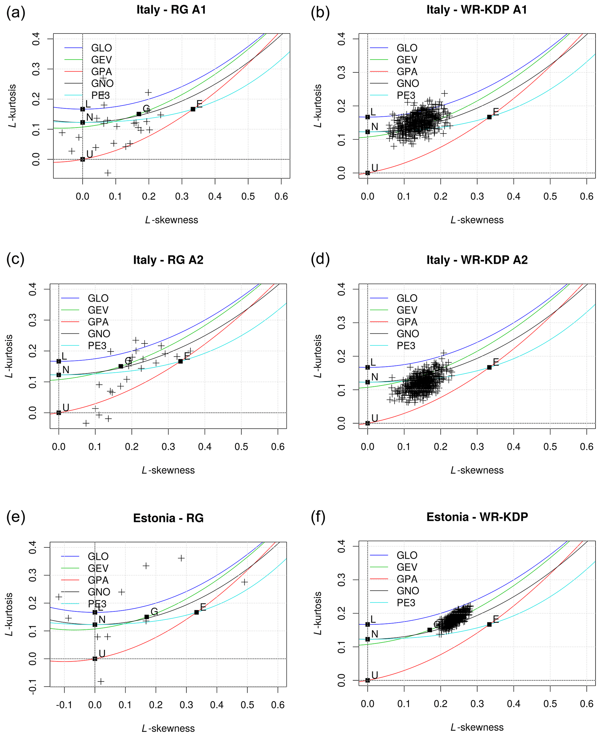
Figure 2 L-moment ratio diagrams for rain gauges (a, c, e) and for QPE weather-radar-based data (d, e, f).

Identifying the best probability distribution for describing the behavior of the annual maxima data is one issue. Plots of L–skewness and L–kurtosis values from both rain gauges and weather radar for the three study areas with a 1 h duration have been elaborated. In order to select the appropriate frequency distribution function, the L-moment ratio diagram method has been used. The L-moment ratio diagram is a widely used tool for the graphic interpretation and comparison of the sample L-moment ratios, L-Cs (skewness), and L-Ck (kurtosis) of various probability distributions (Hosking and Wallis, 1997). Figure 2 shows the L-moment ratio diagram for rain gauges (left) and for weather-radar-based QPEs (right). The right panels of L-moment ratios have been derived from sampling weather-radar-based QPEs 500 times by random uniform sampling. The closeness of the regional mean and the at-site data for the three study areas and for rain gauges and weather-radar-based data to the GEV distribution is evident. Accordingly, a goodness-of-fit test statistic (Hosking and Wallis, 1997) was used in identifying the best three-parameter theoretical distribution. The goodness-of-fit test is based on a comparison between the L-Ck sample and the L-Ck population for different distributions. An acceptable distribution function should achieve a value of Z_DIST≤1.64. For all the datasets of 1 h annual precipitation maxima derived from rain gauges or from weather radar, the Gumbel distribution is acceptable.

2.3 Extreme-value distributions

The statistics of extreme values describe the behavior of the largest of m values: large and consequently rare values are considered extreme. The fundamental result from the theory of extreme-value statistics asserts that, regardless of the (single, fixed) distribution from which the observations have come, the largest of m independent observations from a fixed distribution will match a known distribution more closely as m increases (extremal types theorem; Coles, 2001). Extensive literature, dating back to the 1940s, deals with extreme-value theory in its formalization and its hydrological applications: an introduction to the theory and a historical review on this topic can be found in Papalexiou and Koutsoyiannis (2013), Wilks (2011), and De Haan and Ferreira (2006).

Given R_1 h, the random variable of annual maximum rainfall accumulation for an hourly duration, the cumulative distribution function is given by F(z) (Jenkinson, 1955):

$$\begin{array}{}\text{(4)}& F(R_{\mathrm{1}\mathrm{h}}\le z)=\exp \left(-{\left[\mathrm{1}+\mathit{\xi }{\displaystyle \frac{z-\mathit{\mu }}{\mathit{\sigma }}}\right]}^{-}{\displaystyle \frac{\mathrm{1}}{\mathit{\xi }}}\right)\end{array}$$

with

$$-\mathrm{\infty }<\mathit{\xi }<+\mathrm{\infty },\mathit{\sigma }>\mathrm{0},-\mathrm{\infty }<\mathit{\mu }<+\mathrm{\infty },$$

defined as $z:\mathrm{1}+\mathit{\xi }(x-\mathit{\mu })/\mathit{\sigma }>\mathrm{0}$, where μ, σ, and ξ are the location, scale, and shape parameters, respectively.

According to Katz et al. (2002), the GEV distribution, which combines three different statistical families (Gumbel, Fréchet, and Weibull), can fit the extreme dataset with high accuracy.

The GEV distribution unites the Gumbel, Fréchet, and Weibull distributions into a single family to allow a continuous range of possible shapes (Früh et al., 2010; Coles, 2001). These three distributions are known as type I, II, and III extreme-value distributions. The GEV distribution is parameterized with a location parameter (μ), scale parameter (σ>0), and shape parameter (ξ). The GEV distribution is equivalent to type I, II, and III, respectively, when the shape parameter is equal to zero, greater than zero, and lower than zero:

• ξ>0 Fréchet distribution (EV2),

• ξ=0 Gumbel distribution (EV1),

• ξ<0 Weibull distribution (EV3).

Based on the extreme-value theorem, the GEV distribution is the limit distribution of properly normalized maxima of a sequence of independent and identically distributed random variables. Thus, the GEV distribution is used as an approximation to model the maxima of long (finite) sequences of random variables.

Several methods have been developed for the estimation of GEV distribution parameters, including the method of moments (MME), the method of L-moments (LME), the method of probability-weighted moments (PWME), and the method of maximum likelihood (MLE) (Katz et al., 2002; De Haan and Ferreira, 2006). Hereafter, only the MLE method has been used to estimate GEV distribution parameters from sample data.

By inverting Eq. (4), an estimation of extreme quantiles can be obtained being the pth upper quantile of the z distribution given by F(z_p)=1−p, where z_p is the return level correlated to the return period $T=\mathrm{1}/p$. The z_p-versus-$\mathrm{1}/p$ plot is an effective tool to graphically observe the return levels, and it is known as the return level plot.

The shape parameter controls the upper-tail behavior, but it remains difficult to estimate on the basis of short time-series data (a few decades for example): this happens because there are usually few extremes exhibiting much variability. As stated by Lazoglou et al. (2018), the Weibull distribution (negative shape parameter) is not appropriate for precipitation datasets.

The weather-radar-based rainfall annual maxima statistics over the Netherlands calculated by Overeem et al. (2009a) have shown that regional differences in the location parameter exist for most durations. Nevertheless, due to the small number of rainfall annual maxima, when depth–duration–frequency (DDF) curves are derived for small areas, the uncertainties in the DDF curves generally become larger compared to the uncertainties in the average DDF curve for the Netherlands. Recalling an increase in the standard errors of the quantile estimates, in particular for high return periods, Buishand (1991) stresses that large standard errors are mainly caused by the uncertainty in the shape parameter. On the other hand, real-time operational applications, like issuing of early warnings, are based on relatively low quantiles (typically a 10–20-year return period). Within this range of return periods, the inaccuracy is expected to be considerably reduced (Marra et al., 2019): for these reasons in this study, the Gumbel distribution (ξ=0) has been assumed appropriate for 1 h accumulation annual rainfall maxima.

As discussed by Overeem et al. (2009a), the spatial correlation of measurements affects extreme-value statistics, leading to underestimation. The correlation between two rain gauges is typically low for convective precipitation due to the small spatial scales involved in convection (≈ 10–100 km²) and the low density of the ground meteorological network (typically on the order of one gauge every 100 km²). In the case of weather radar observations, given the higher spatial resolution (≈ 1 km²), the correlation between close cell grids must be estimated and taken into account. Assuming GEV distribution parameters are constant in each of the areas considered in this study, their estimation from all data in the regions justifies the derivation of return periods longer than the rainfall record (Overeem et al., 2010). This statement assumes both that sample data are independent and that the precipitation regime in the studied area is uniform. To avoid data spatial correlations, this study merely investigates 1 h rainfall totals, disregarding longer durations.

Semi-variograms are widely used in geostatistical sciences for evaluating rainfall spatial structure. Semi-variograms summarize the spatial relations in the data, and they can be used to understand within what range data are spatially correlated (Naimi et al., 2011).

In this study, the statistical analysis has been conducted using the R (https://cran.r-project.org/, last access: 11 June 2023) package extRemes 2.1 (Gilleland and Katz, 2016). The experimental isotropic semi-variogram can be derived by taking half the average of the squared difference between data pairs at equal distances and by assuming stationarity and isotropy of the rainfall field (Cressie, 1993):

$$\begin{array}{}\text{(5)}& \mathit{\gamma }\left(h\right)={\displaystyle \frac{\mathrm{1}}{\mathrm{2}n\left(\right|h\left|\right)}}\sum _{k=\mathrm{1}}^{n\left(\right|h\left|\right)}{\left(z(x_k+h)-z\left(x_k\right)\right)}^{\mathrm{2}},\end{array}$$

where x_k is the location of cell barycenter k and x_k+h is the location at distance h from location x_k.

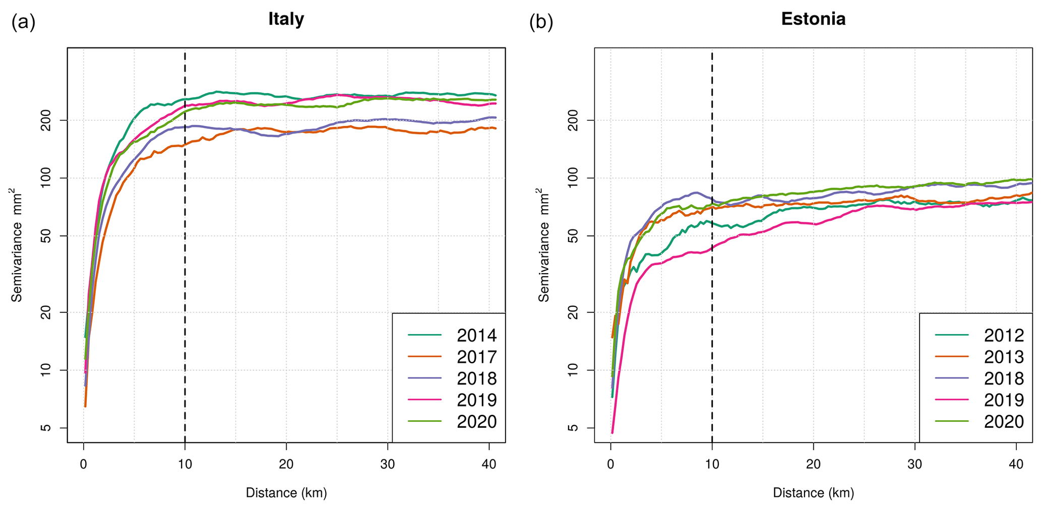
Figure 3 Empirical variograms for hourly rainfall annual maxima based on R(Z_h,K_dp) hourly rainfall estimations in Italy area A1 (a) and Estonia (b).

Figure 3 shows semi-variograms, obtained from R(Z_h,K_dp) annual hourly rainfall maxima, from April to September in Italy for area A1 (left) and Estonia (right).

The empirical semi-variogram analysis for weather radar observations indicates that hourly rainfall maxima decorrelate at about 10 km in both Estonia and Italy (Fig. 3). These results are consistent with past studies (Schroeer et al., 2018; Dzotsi et al., 2013): convective precipitation is prevalent during the warm season, and, consequently, the spatial correlation quickly decreases with the distance between two rain gauges. Moreover, 10 km is the typical spatial scale of convective precipitation systems (meso-γ). Different values of semi-variances in Estonia and Italy can be explained by the different climatic regimes, with generally weaker convective-precipitation events in the Baltic country. Hence, to avoid statistical oversampling and to ensure the statistical independence of data samples, 1 h rainfall total annual maxima estimated by weather radar are re-sampled according to the spatial scale of convective precipitation found. The hourly annual rainfall maxima estimated by weather radar observations are upscaled from the original data resolution (340 m for Italy and 300 m for Estonia) to 10 km resolution, using a uniform random sampling algorithm.

3 Results

On the basis of the goodness-of-fit results, the observations relative to all three study areas have been fitted with Gumbel distributions. For weather radar QPEs, the fit has been performed considering the mean L-moments, derived from random sampling 500 times the original data at 10 km resolution. Figure 4 shows the diagnostics from the Gumbel distribution fitted to 1 h rainfall total annual maxima in Italy for area A1 (upper) and Estonia (lower), derived from R(Z_h,K_dp) estimates; from left to right, the figure shows the density plot of the data along with the model-fitted density, a Q–Q plot of quantiles from model-simulated data against the data quantiles with 95 % confidence bands. Quantile–quantile scatterplots compare empirical data and fitted cumulative distribution functions (CDFs) in terms of quantiles: in an ideal perfect fitting, all points should lie on the 1 : 1 diagonal line (Wilks, 2011).

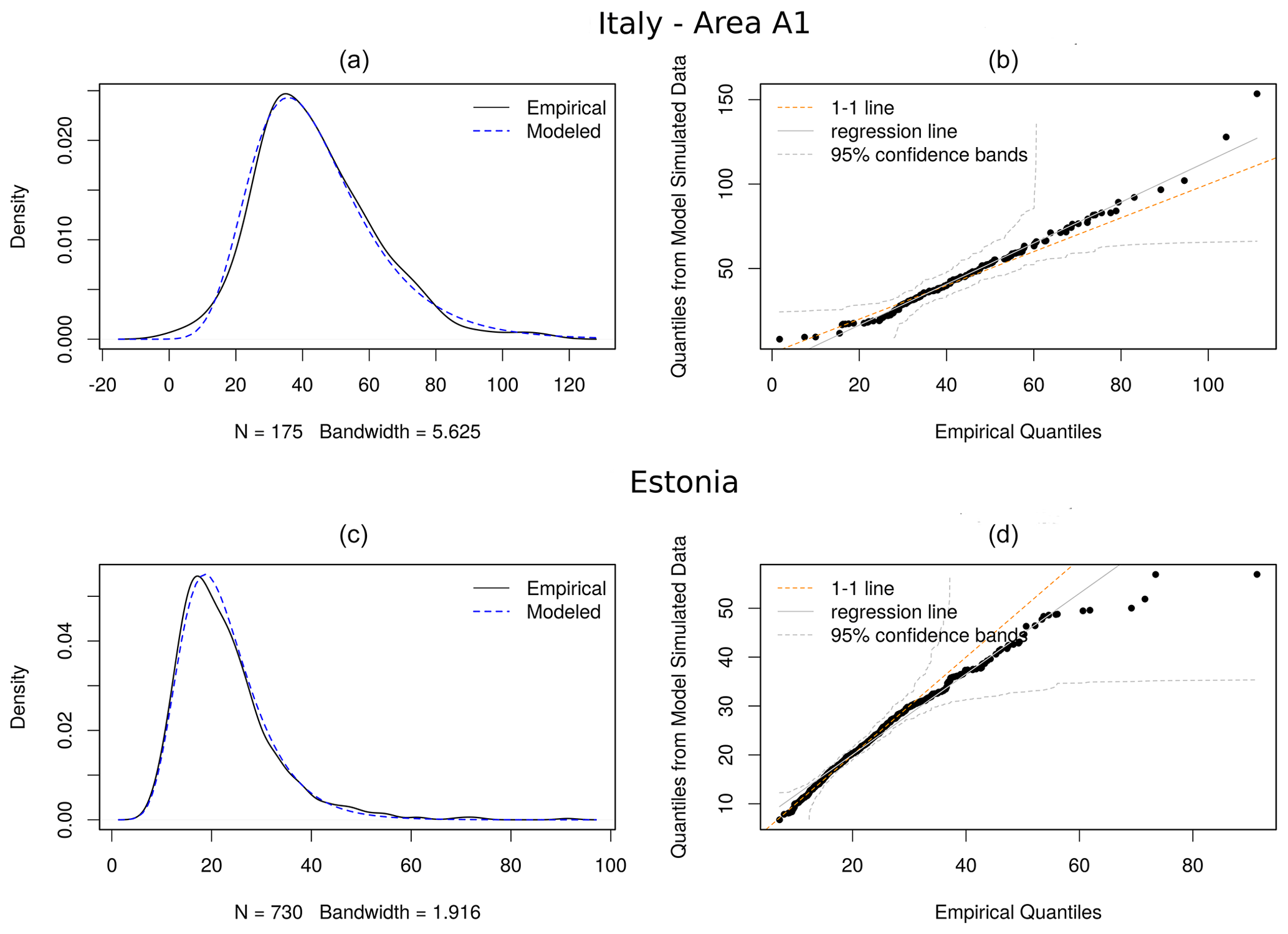
Figure 4 Diagnostic plots for 1 h annual rainfall maxima fits derived by weather radar in Italy area A1 (a, b) and Estonia (c, d): from left to right, density plot of the data along with the model-fitted density, Q–Q plot of the data quantiles from model-simulated data against the data quantiles with 95 % confidence bands.

The Q–Q plots present some departures from linearity in correspondence to the tails, especially for Estonia data, which are due to the increasing level of uncertainty that characterizes model extrapolation at high levels. The empirical estimates in the return level plot reflect results in Q–Q plots lying very close to the model-based line, with results being almost linear for low values. However, even if the return level estimates seem convincing, the increasing confidence bands for large return periods indicate the uncertainty that affects the model at high levels.

Table 1 summarizes the results of fitting data samples with Gumbel distributions by applying the maximum likelihood estimation method (MLE) for each studied area; location and scale parameters with their standard errors ($\mathit{\sigma }/\sqrt{n}$ are shown. Kolmogorov–Smirnov tests (KS tests) and Q–Q plots inspections (Wilks, 2011) show that fits for R(Z_h,K_dp) are more reliable than R(Z_h) ones in all three study areas. This behavior is particularly evident for the Estonia area, where the fit distribution for R(Z_h) leads to a large value of the scale parameter and an anomalously low p value obtained by KS tests.

Table 1 Estimated Gumbel parameters, location, and scale (μ,σ) for weather radar and gauge annual hourly maxima rainfall intensities for Italy area A1 and area A2 and Estonia for weather radar derived from R(Z_h,K_dp) (WR-KDP) and from R(Z_h) (WR-ZH) and rain gauge (RG) time-series observations.

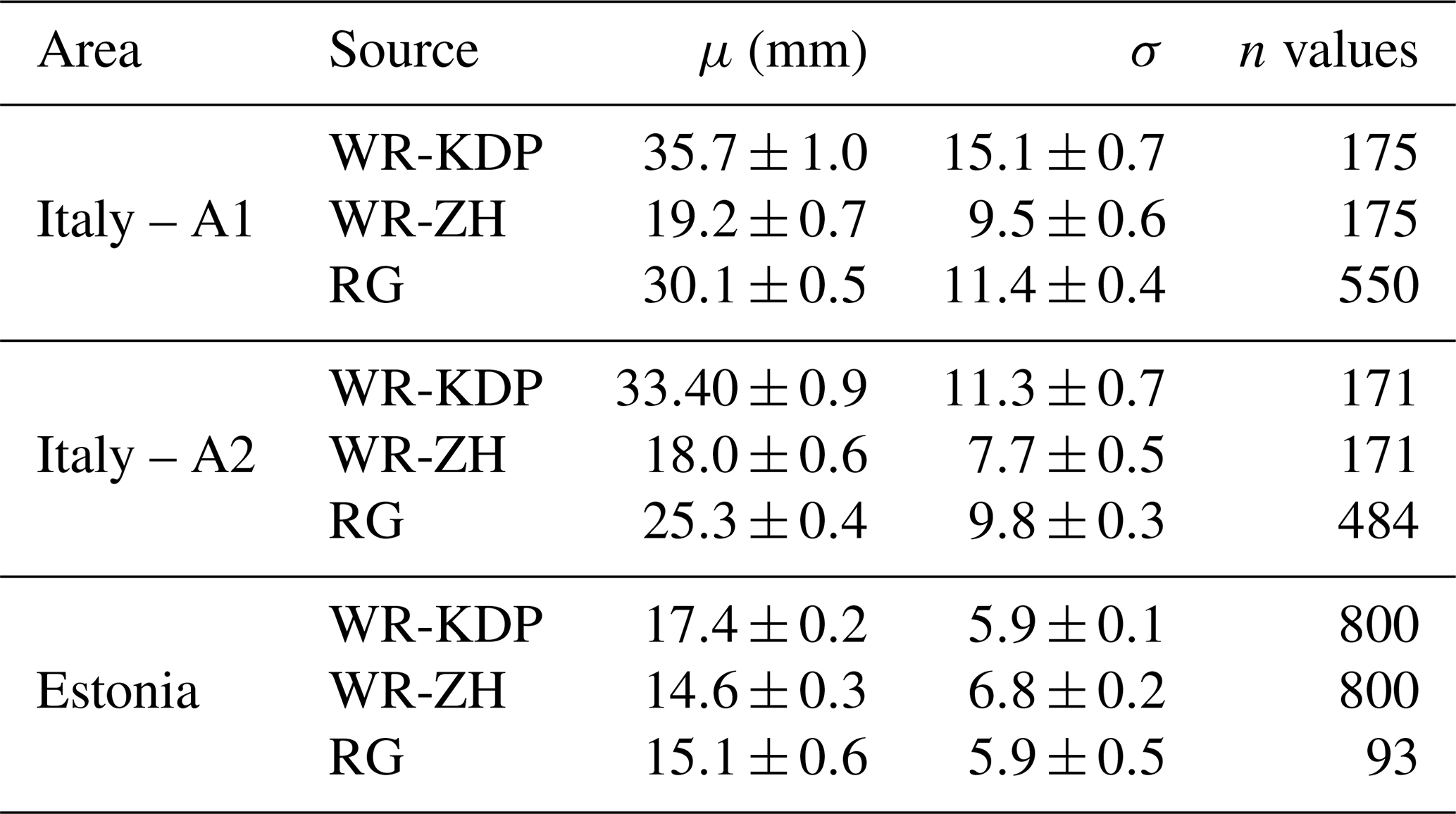
It is well-known that record length affects the estimate of the GEV shape parameter and that long historical time series are needed for reliable estimates. Papalexiou and Koutsoyiannis (2013), Ragulina and Reitan (2017), Lazoglou et al. (2018), Lutz et al. (2020), and Deidda et al. (2021) demonstrated that the shape parameter tends to have positive values, between 0 and 0.23 with a probability of 99 %, as sample size increases. However, in this study, given the shortness of the weather radar time series, for safety the scale parameter has been set to zero, according to Papalexiou and Koutsoyiannis (2013).

4 Discussion

Several studies have developed adjustment techniques to correct QPEs based on weather radar observations with rain gauge measurements (Einfalt and Michaelides, 2008; Goudenhoofdt and Delobbe, 2009). For the first time, this study investigates extreme precipitation estimation using dual-polarization weather radar rainfall estimations without any adjustment with rain gauges. It is worth recalling that the study has been limited to relatively flat and geomorphologically homogeneous areas with high-quality dual-polarization weather radar observations close to the ground and high-quality 1 h rainfall total annual maxima from rain gauges. Weather radar data quality and reliability have been carefully checked in Voormansik et al. (2021a).

The two studied regions, Estonia and Italy, are characterized by different precipitation regimes, the first one colder and the latter warmer. The different climate regimes of the studied areas consequently reflect on fitted Gumbel distributions, determining lower return periods in Italy, given a 1 h rainfall total. Estonia is characterized not only by few rain gauges and by a limited historical series but also by a larger homogeneous, flat region covered by the operational polarimetric weather radar. In this area, the benefit of estimating Gumbel distributions using weather radar observations after ensuring spatial independence and assuming homogeneity can be appreciated: the sample size derived from 5 years of observations is about 9 times the sample size obtained by rain gauges. These different sample sizes determine larger standard deviations in Gumbel distribution parameter estimation by rain gauges with respect to weather-radar-based estimations.

In Italy, a dense automatic gauge network has been operating since 1988, providing about 25 gauges per area and determining a larger sample size. But the Alps and the spatial variability in the climate regime, influenced by complex orography, limit the availability of high-quality weather radar observations to about 160–180 values. Despite the limited availability of weather radar observations (only 5 years for both Italian and Estonian weather radars), the comparison of Gumbel distribution fits in these two different regions has shown encouraging results.

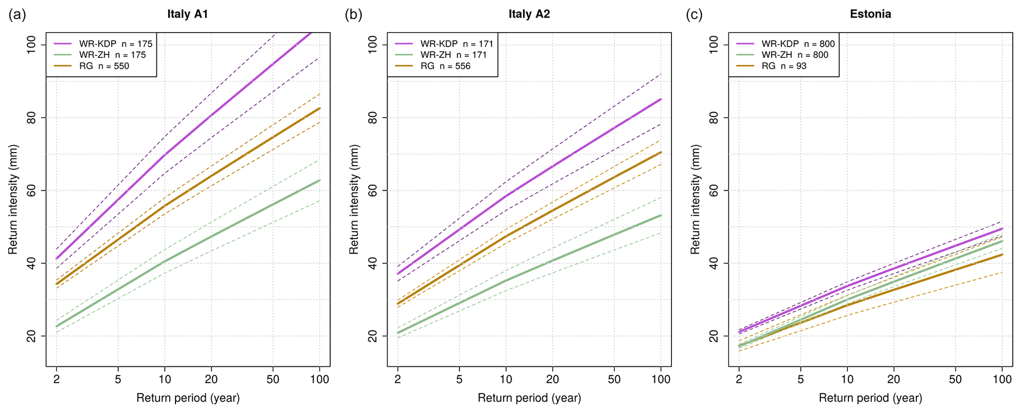
Figure 5 Return levels for 1 h rainfall accumulation in Estonia (a) and Italy area A1 (b) and Italy area A2 (c) derived from the Gumbel distributions. The dashed lines show confidence intervals for α=0.05.

Figure 5 shows return levels for 1 h rainfall at a given return time, estimated from Gumbel distributions with location and shape parameters from Table 1 for the study areas and estimated from R(Z_h), R(Z_h,K_dp) and from rain gauges.

Table 2 The return time period estimates for 1 h rainfall accumulation for the three study areas, derived from R(Z_h), R(Z_h,K_dp), and rain gauges.

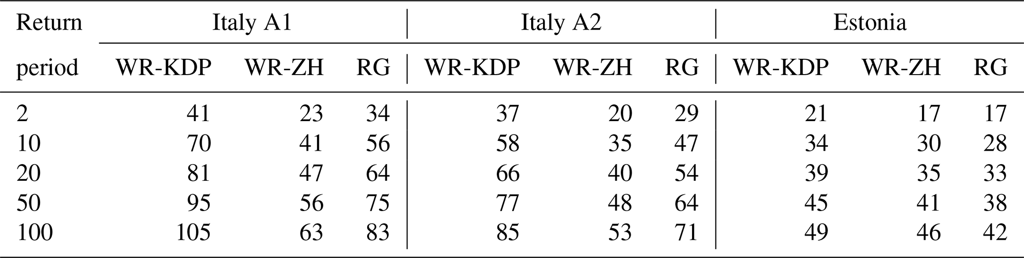
In Italy, the different return periods between the two areas are in agreement with findings in Mezzoglio et al. (2022) and with climate classification of the two areas reported by Pavan et al. (2018), with area A1 more favorable to intense precipitation than area A2. This precipitation regime, confirmed also by climatological lightning density (not shown), can be justified by local geomorphology. In fact, during the warm season, cold air comes over the Alps flowing towards the Po Valley from west-northwest: the Monferrato hills east of Turin enhance low-level convergences and strong uplifts, causing deep convection in area A1, while study area A2 experiences downwind conditions. QPEs based on the Z_h–K_dp algorithm generally provided slightly shorter return periods with respect to gauge estimations; this behavior can be explained by the high spatial resolution of weather radar observations able to catch small-scale rain showers. However, it could also be due to a slight overestimation of annual rainfall maxima by weather radars, as highlighted by Voormansik et al. (2021a), and hence needs further investigations. The distribution fits based on R(Z_h) show a longer return period, given a 1 h rainfall total, in all three areas. This return period overestimation is dramatic in Italy, where a higher 1 h rainfall maxima total is expected. Table 2 summarizes the return time period estimates for 1 h rainfall accumulation for the three study areas, derived from R(Z_h), R(Z_h,K_dp), and rain gauges.

The maximum 1 h accumulation for a given return time obtained from R(Z_h,K_dp) shows better agreement with values obtained by rain gauges. In the two Italian areas, the underestimation by R(Z_h) is evident and larger in area A1 than in area A2. For Estonia, R(Z_h,K_dp) confirms good performance, while R(Z_h) confirms underestimation but also shows an unrealistic large-scale parameter and a low statistical significance of the fit. Recalling the findings in Voormansik et al. (2021a), QPEs derived by Z_h show underestimation during the warm season. However, several reasons can explain the weakness of R(Z_h):

1. horizontal radar reflectivity attenuation caused by intense instantaneous rainfall rates,

2. partial beam filling,

3. inappropriate reflectivity cap threshold (55 dBZ) to avoid hail contamination (disdrometer measurements reported cases of rainfall rates greater than 100 mm h⁻¹),

4. clutter residual,

5. inappropriate drop size distribution assumed to convert weather radar horizontal reflectivity into the rain rate.

On the other hand, R(Z_h,K_dp) estimations outperform in a strongly convective-precipitation regime like in northern Italy, being immune from hail contamination and rainfall attenuation.

The major advantages of using weather radars for such applications are that information for unmeasured locations can be obtained and spatial gradients of the variables of interest captured. Due to the limited polarimetric weather radar data availability in time (a few years), the present study is limited to climatologically homogeneous areas, limiting or losing these advantages. Nevertheless, previous studies (Overeem et al., 2008, 2009a, b, 2010; Marra and Morin, 2015; Panziera et al., 2018; Marra et al., 2022) have analyzed weather radar QPEs based on horizontal reflectivity data adjusted with some ground rain gauge measurements. Here, the major innovative aspect is that the QPEs, based on the blended algorithm R(Z_h,K_dp), are obtained independently of co-located rain gauge data availability. This study demonstrates that, by having polarimetric rainfall estimates, it is possible to estimate the rainfall annual maxima even in ungauged regions. Moreover, as stated by Marra and Morin (2015), dealing with QPEs based on radar reflectivity factor data, the upper threshold used to limit hail contamination is an issue in rainfall maxima estimation in warm regions, limiting the instantaneous rainfall estimation typically to about 100 mm h⁻¹. Involving K_dp for QPEs, the hail contamination issue is overcome, making QPEs independent of both climatic region and weather radar attenuation. Future studies will benefit from longer time series allowing investigations in wider non-homogeneous areas.

5 Conclusions

Several studies have investigated rainfall annual maxima derived from weather-radar-based QPEs obtained by the traditional Z_h–R relationship with some adjustments with rain gauges. In the past decades, dual-polarization weather data radar observations have become available from operational weather radars. As stated by Bringi and Chandrasekhar (2001) and Voormansik et al. (2021a), the benefits of using dual-polarization variables like K_dp in rainfall estimates are evident: these QPEs are immune from weather radar miscalibration, anomalous propagation, and partial beam blocking or beam filling.

For the first time, this study investigates QPEs based on polarimetric observations by operational C-band weather radar located in Italy and Estonia. The most remarkable aspects of this study are that

• data are derived from operational C-band weather radar without any dedicated settings,

• QPEs are derived by polarimetric observations without any rain gauge adjustments.

As shown by Voormansik et al. (2021a), rainfall estimations based on Z_h–K_dp algorithms are robust and reliable, overcoming most of the sources' uncertainties; hence, no corrections or adjustments with rain gauges have been applied. The annual maximum of 1 h rainfall accumulation is typically assumed to have a GEV distribution. Given the shortness of weather radar data, this study is limited to a short duration (1 h) in homogeneous regions assuming parent Gumbel distributions. Hence, Gumbel distribution parameters and depth–frequency curves have been derived from the 1 h dual-polarization weather-radar-based annual rainfall maxima. The comparison of weather radar return period estimations with ones derived from gauge observations showed a good agreement. This study demonstrates that thanks to weather radar high spatial resolutions, even a limited time series of weather radar observations can provide reliable estimations of extreme-value-distribution parameters for annual hourly rainfall maxima in climatologically homogeneous regions. It is worth recalling that QPEs based on R(Z_h−K_dp) observations can be obtained only in cases of warm-season precipitation events (when most intense precipitation events occur anyway). The results shown demonstrate good agreement between QPEs obtained by R(Z_h−K_dp) and rain gauge data and consistent estimations of Gumbel distribution parameters. Assuming homogeneous regions with high-quality weather radar observations, it is shown that even limited time-series weather radar observations can discriminate 1 h rainfall total annual maxima between different precipitation regimes. These results are promising especially if we recall that the two areas in Italy are characterized by slightly different precipitation regimes and the applied statistical analysis can describe them properly. The main requirements for weather radar observations applying this approach consist of proper weather radar calibration, radar visibility, and a limited beam broadening united to a limited beam height above the ground.

As longer rainfall time series based on dual-polarized meteorological data become available, more investigations into different rainfall durations in wider and non-homogeneous areas will be possible, allowing estimations of spatial gradients and evaluations of different statistical distributions. Sub-hourly precipitation extremes can determine a wide range of impacts on infrastructure, economy, and even health, causing urban flooding and triggering landslides, flash floods, and heavy soil erosion. Hence, future works will focus on sub-hourly rainfall accumulation intervals, estimating GEV parameter distributions and deriving other significant return periods.