Global evaluation of Doppler velocity errors of EarthCARE cloud-profiling radar using a global storm-resolving simulation

The cloud-profiling radar (CPR) on the Earth Clouds, Aerosol, and Radiation Explorer (EarthCARE) satellite (EC-CPR) is the first satellite-borne Doppler radar. In a previous study, we examined the effects of horizontal (along-track) integration and simple unfolding methods on the reduction of Doppler errors in the EC-CPR observations, and those effects were evaluated using two limited scenes in limited-latitude and low-pulse-repetition-frequency (PRF) settings. In this study, the amount of data used was significantly increased, and the area of the data used was extended globally. Not only low-PRF but also high-PRF settings were examined. We calculated the EC-CPR-observed Doppler velocity from pulse-pair covariances using the radar reflectivity factor and Doppler velocity obtained from a satellite data simulator and a global storm-resolving simulation. The global data were divided into five latitudinal zones, and each standard deviation of Doppler errors for 5 dBZ_e after 10 km integration was calculated. In the case of the low-PRF setting, the error without unfolding correction for the tropics reached a maximum of 2.2 m s⁻¹ and then decreased toward the poles (0.43 m s⁻¹). The error with unfolding correction for the tropics became much smaller at 0.63 m s⁻¹. In the case of the high-PRF setting, the error without unfolding correction for the tropics reached a maximum of 0.78 m s⁻¹ and then decreased toward the poles (0.19 m s⁻¹). The error with unfolding correction for the tropics was 0.29 m s⁻¹, less than half the value without the correction. The results of the analyses of the simulated data indicated that the zonal mean frequency of precipitation echoes was highest in the tropics and decreased toward the poles. Considering a limitation of the unfolding correction for discrimination between large upward velocity and large precipitation falling velocity, the latitudinal variation in the standard deviation of Doppler error can be explained by the precipitation echo distribution.

1 Introduction

The Earth Clouds, Aerosol, and Radiation Explorer (EarthCARE; hereafter EC) is a joint satellite mission by the Japan Aerospace Exploration Agency (JAXA) and the European Space Agency (ESA) that will carry a cloud-profiling radar (CPR), an atmospheric lidar (ATLID), a multispectral imager (MSI), and a broadband radiometer (BBR). From the derived 3D cloud and aerosol scene profiles, heating rates and radiation flux profiles are systematically determined with a resolution of 100 km² (Illingworth et al., 2015). Active sensors of EC will be regarded as an evolutional successor of the 94 GHz CloudSat CPR (Stephens et al., 2008) and the Cloud-Aerosol Lidar and Infrared Pathfinder Satellite Observations (CALIPSO; Winker et al., 2009) lidar (Stephens et al., 2018).

Because of EC's low orbit (∼ 400 km) and the EC-CPR's large antenna (2.5 m), it has a better sensitivity (−36 dBZ_e at the top of the atmosphere – TOA) than the CloudSat CPR (−30 dBZ_e) and can observe 98 % of radiatively significant ice clouds and 40 % of all stratocumulus clouds (Stephens et al., 2002; Hagihara et al., 2010). Moreover, the EC-CPR has a vertical Doppler measurement capability that the CloudSat CPR does not have. It will reveal, for the first time, the vertical motion of cloud particles globally. Such an entirely new dataset would improve the discrimination between clouds and precipitation (Ceccaldi et al., 2013; Kikuchi et al., 2017) as well as the retrieval of cloud microphysical parameters (Heymsfield et al., 2008). Consequently, it should improve various parameterization schemes used in atmospheric models and the understanding of the processes related to cloud and precipitation (Roh and Satoh, 2014, 2018; Roh et al., 2017; Hagihara et al., 2014; Mülmenstädt et al., 2020; Takahashi et al., 2021).

Vertical Doppler velocity estimation from space suffers from Doppler broadening and velocity folding or aliasing (e.g., Kobayashi et al., 2002; Sy et al., 2014). The EC-CPR measures Doppler velocities using the pulse-pair method. It measures the phase shift in echoes from two successive transmitted pulses. As the EC-CPR is a finite beamwidth on a fast-moving spaceborne platform, targets have a broad Doppler width, which causes a worsening of the correlation of the phase. Then, large Doppler errors are introduced. Hagihara et al. (2022; hereafter H22) examined the effect of horizontal (along-track) integration and unfolding methods on the reduction of Doppler velocity measurement errors, in order to improve Doppler data processing in the JAXA standard algorithm. They obtained EC-CPR data simulated by a satellite data simulator, the Joint-Simulator (Hashino et al., 2013, 2016; Satoh et al., 2016; Roh et al., 2020), using global storm-resolving simulation data with the Nonhydrostatic ICosahedral Atmospheric Model (NICAM; Tomita and Satoh, 2004; Satoh et al., 2008, 2014). They evaluated the standard deviation (SD) of the random errors for each Z_e for two cases (cirrus clouds and precipitation). They found that the error was reduced by horizontal integration alone in the case of cirrus clouds, whereas the error became large without unfolding correction in addition to the horizontal integration in the case of precipitation.

In H22, the evaluation was limited to two scenes in the midlatitudes of the Northern Hemisphere and a low-pulse-repetition-frequency (PRF) setting. In this study, we used more data than in H22 and performed the evaluation on a global scale. We also adopted different PRF settings. In Sect. 2, the simulation methods for EC-CPR data, the horizontal integration and unfolding correction of Doppler velocity, and the CloudSat-observed data are described. In Sect. 3, we investigate the SD of the random errors on a global scale. To examine the characteristics of each latitude, we separated the data into five latitudinal zones. Two PRF modes were also included. The summary and conclusions are given in Sect. 4.

2 Data and method

We utilized the global hydrometer data simulated by the global storm-resolving model NICAM with a 3.5 km horizontal resolution. Moreover, we obtained the simulated EC-CPR data using the aforementioned data and the Joint-Simulator, following H22. Note that attenuations of gas and particles are considered in the calculation of the radar reflectivity factor, whereas Doppler velocity is the total velocity of the hydrometer echo, including reflectivity-weighted particle fall speed and vertical air motion. Our forward model is based on the single-scattering assumption. There are some studies on multiple scattering using Monte Carlo methods (e.g., Matrosov et al., 2008; Battaglia and Tanelli, 2011). Specifically, the effect of multiple scattering on the Doppler velocity is discussed in Battaglia and Tanelli (2011). In this study, we focus on Doppler errors caused by Doppler broadening and folding; therefore, for simplicity, we do not consider multiple scattering. This issue will be the subject of future research. The simulated data were then calculated along an EC orbit and interpolated into the EC-CPR sampling interval (100 m in the vertical and 500 m in the horizontal). The radar reflectivity factor (Z_e, jsim) and Doppler velocity (V_jsim) curtain data were obtained (hereinafter referred to as “NICAM/J-Sim data”). In H22, only two scenes extracted from two orbits of data were used; however, in this study, the amount of data used was significantly increased to 16 orbits of data, which is equivalent to 1 d of satellite tracks.

We note that there may be fast updrafts on the kilometer or sub-kilometer scale. However, such events are rare globally and would be negligible in statistics such as latitudinal zonal means. This study focuses on global statistical results; therefore, we use the NICAM. When higher horizontal resolution NICAM data become available, we would like to study similar evaluation using them.

In using the NICAM/J-Sim data, we first performed the following statistical analyses. We examined the zonal mean frequencies of hydrometeors obtained from the NICAM/J-Sim data and the CloudSat observations for 19 June 2008 (Fig. 1). We used the CloudSat Z_e (the standard geometrical profile of the cloud product, 2B-GEOPROF) (Stephens et al., 2008) for comparison with Z_e, jsim. For the observed data, we defined the hydrometeor bin as where the cloud mask value is greater than or equal to 20 from the CPR 2B-GEOPROF product, which means a weak, good, or strong echo detection (Marchand et al., 2008). These are estimated to give an estimated false-detection rate smaller than 5 %. This value is adopted in many other CloudSat-based hydrometeor studies (e.g., Sassen and Wang, 2008). The frequency of cloud occurrence at a given altitude was defined as the number of cloud echo bins ($Z_{\mathrm{e}}>-\mathrm{24}$ dBZ_e) divided by the total number of observations at that level. The bin size was 240 m in the vertical and 2.0^∘ latitude in the horizontal. The overall frequencies of the NICAM/J-Sim-simulated cloud field are comparable to the results of the CloudSat observations.

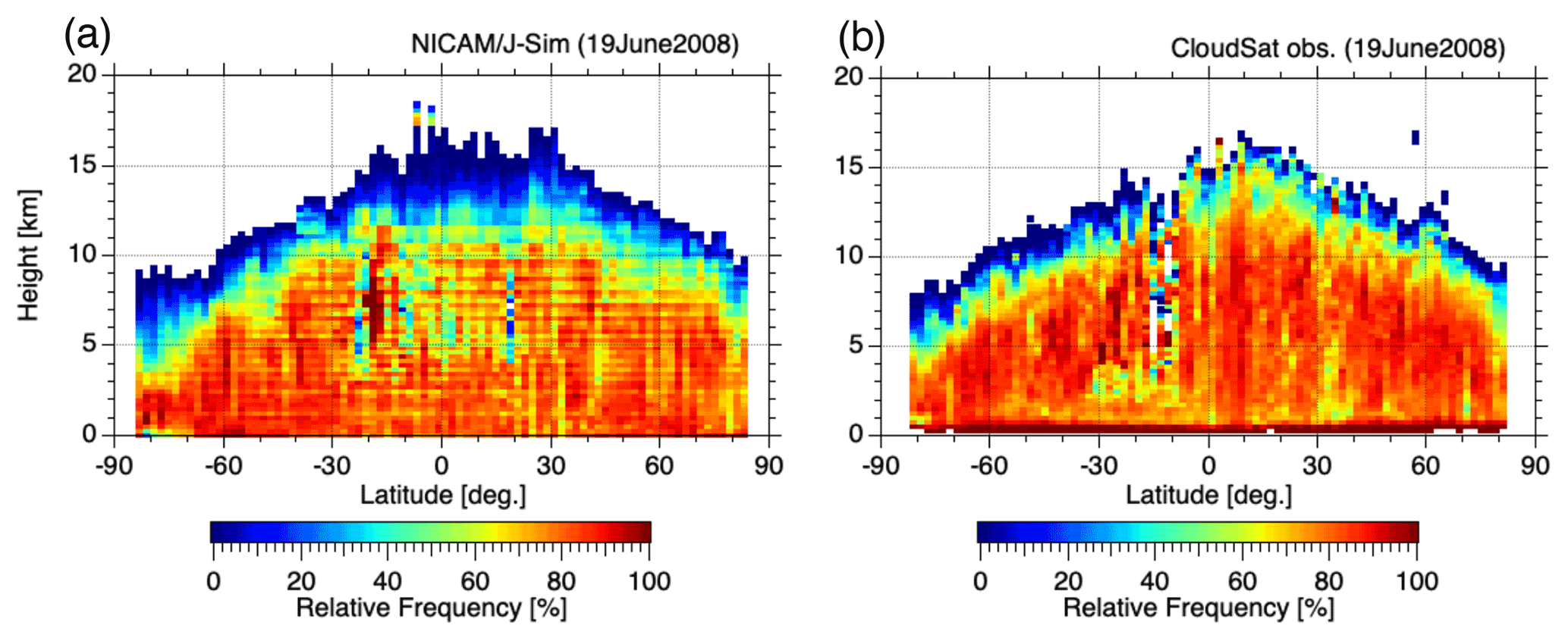
Figure 1 Zonal mean frequency of hydrometeors obtained by (a) NICAM/J-Sim and (b) CloudSat observations for 19 June 2008.

We simulated the measured vertical Doppler velocity (V_m) as

$$\begin{array}{}\text{(1)}& V_{\mathrm{m}}=V_{\mathrm{jsim}}+V_{\mathrm{random}},\end{array}$$

where V_random is the random error caused by the spread of Doppler velocities within the beam width. This is a Gaussian error distribution, and its SD of the random error (SD_random) is determined by perturbation approximation (Doviak and Zrnic, 1993) as

$$\begin{array}{}\text{(2)}& {\mathrm{SD}}_{\mathrm{random}}=C\sqrt{{\displaystyle \frac{{\mathit{\lambda }}^{\mathrm{2}}}{\mathrm{32}{\mathit{\pi }}^{\mathrm{2}}M\cdot {\mathit{\rho }}^{\mathrm{2}}\cdot {\left(\frac{\mathrm{1}}{\mathrm{PRF}}\right)}^{\mathrm{2}}}}\left[{\left(\mathrm{1}+{\displaystyle \frac{N}{S}}\right)}^{\mathrm{2}}-{\mathit{\rho }}^{\mathrm{2}}\right]},\end{array}$$

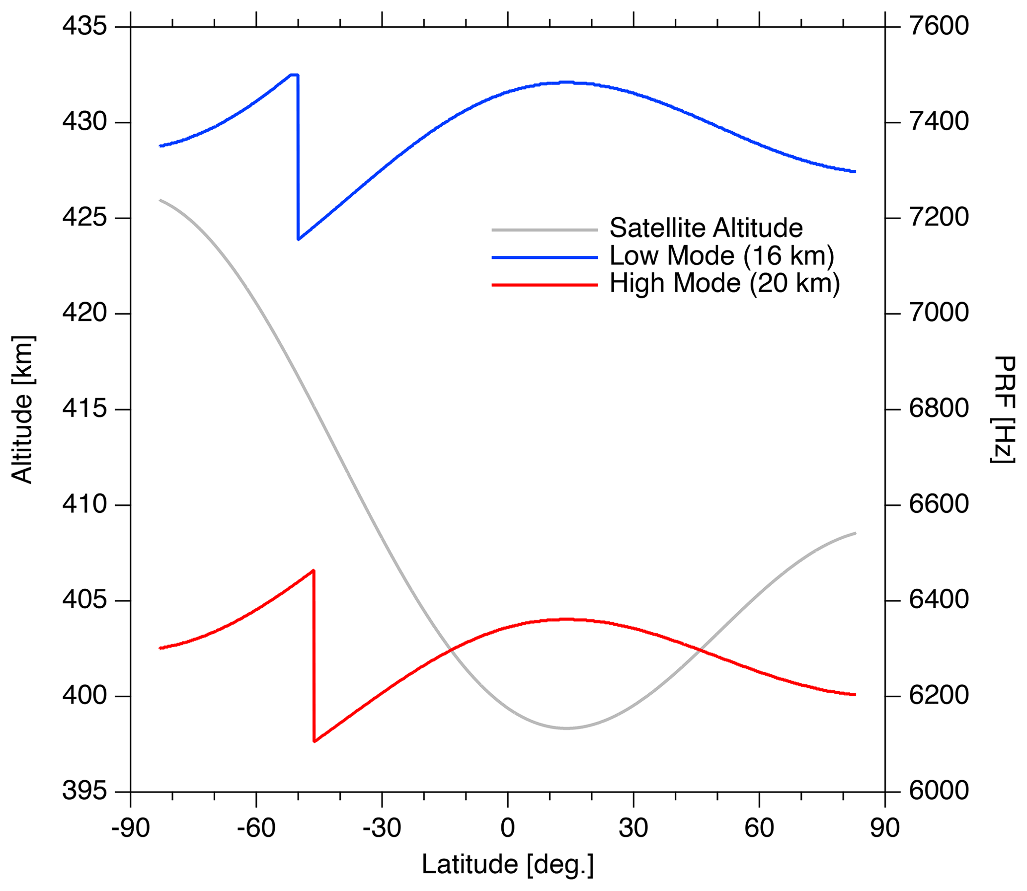
where C is a correction factor. We set C=1.3 following H22. The wavelength is λ (λ=3.2 mm for EC-CPR), M is the number of pulse pairs within an integration length, ρ is the correlation function, and $S/N$ is the signal-to-noise ratio (SNR). In nominal operation, the EC-CPR will change the observation window – that is, low mode (−1 to 16 km altitude) at latitudes of 60–90^∘ and high mode (−1 to 20 km) at latitudes of 0–60^∘. The PRF is determined on the basis of the satellite altitude and changes in the range of 6100 to 7500 Hz with the latitude and observation window, as illustrated in Fig. 2. The high mode has a lower PRF and worse Doppler accuracy, as discussed in H22, although cloud echoes up to an altitude of 20 km can be observed. On the other hand, the low mode has a higher PRF and better Doppler accuracy, but cloud echoes higher than 16 km cannot be observed. M is 357 to 420 for 500 m integration depending on the PRF. The SNR is determined by the received echo power calculated from the radar equation and estimated EC-CPR noise level. In the case of EC-CPR, the SNR is 0 dB, which is a signal equivalent to a −21.2 dBZ_e echo intensity. If Z_e, jsim is less than −24 dBZ_e, we assume the Doppler velocity of its echo to be random noise in this study. The correlation function ρ is defined as

$$\begin{array}{}\text{(3)}& \mathit{\rho }=\exp \left\{-\mathrm{8}{\left({\displaystyle \frac{\mathit{\pi }\cdot {\mathit{\sigma }}_v}{\mathit{\lambda }\cdot \mathrm{PRF}}}\right)}^{\mathrm{2}}\right\},\end{array}$$

where σ_v is the total Doppler velocity spectrum width.

Figure 2 Satellite altitude and the PRF as functions of latitude and observation mode.

The width σ_v can be considered to be a sum of contributions by each. Thus,

$$\begin{array}{}\text{(4)}& {\mathit{\sigma }}_v^{\mathrm{2}}={\mathit{\sigma }}_{\mathrm{sm}}^{\mathrm{2}}+{\mathit{\sigma }}_{\mathrm{t}}^{\mathrm{2}}+{\mathit{\sigma }}_{\mathrm{psd}}^{\mathrm{2}},\end{array}$$

where σ_sm is the spread due to satellite motion, given by σ_sm∼0.3 V_satθ_3 dB; V_sat is the satellite velocity; and θ_3 dB is the beam width (Sloss and Atlas, 1968). When V_sat is 7738 m s⁻¹ and θ_3 dB is 0.00166 rad (0.095^∘), σ_sm becomes 3.85 m s⁻¹. The spread σ_t and σ_psd are due to turbulence and the distributions of hydrometeor falling velocities, respectively, which are assumed to have respective values of σ_t=1.0 m s⁻¹ (Amayenc et al., 1993) and σ_psd=0.5 m s⁻¹ (Gossard et al., 1997). As for the latter term, it is reported to spread to 1.0 m s⁻¹ for rain (Lhermitte, 1963). In this study, we assumed that σ_psd = 0.5 m s⁻¹ so that σ_v becomes 4.01 m s⁻¹.

The EC-CPR measures the phase change in the echo between two successive pulses by pulse-pair processing to estimate the Doppler velocities. The real and imaginary parts of pulse-pair covariances R_τ integrated onboard, corresponding to 500 m along track, are simulated in this study as follows:

$$\begin{array}{}\text{(5)}& \mathrm{Re}\left(R_{\mathit{\tau }}\right)=Z_{\mathrm{e},\mathrm{jsim}}\cdot \cos \left({\displaystyle \frac{\mathrm{4}\mathit{\pi }\cdot V_{\mathrm{m}}}{\mathit{\lambda }\cdot \mathrm{PRF}}}\right),\end{array}$$

$$\begin{array}{}\text{(6)}& \mathrm{Im}\left(R_{\mathit{\tau }}\right)=Z_{\mathrm{e},\mathrm{jsim}}\cdot \sin \left({\displaystyle \frac{\mathrm{4}\mathit{\pi }\cdot V_{\mathrm{m}}}{\mathit{\lambda }\cdot \mathrm{PRF}}}\right).\end{array}$$

V_500 m is calculated using the arctangent of the real and imaginary parts of the 500 m integrated R_τ simulated by Eqs. (5) and (6). The sign of the Doppler velocity is defined as being that of the radial Doppler velocity (i.e., downward motion is positive) following the EC-CPR data processing. To reduce random error, V_1 km and V_10 km are also calculated using the 1 and 10 km horizontally integrated R_τ values, respectively, that are calculated from the 500 m integrated R_τ.

Velocity folding or aliasing is inherent to Doppler radar. V_max can be measured by the pulse-pair method and is defined by PRF ($V_{\max }=\mathit{\lambda }\cdot$ PRF/4). In the PRF of the high mode (lower PRF), V_max ranges from 4.9 to 5.2 m s⁻¹, whereas in the PRF of the low mode (higher PRF), it ranges from 5.7 to 6.0 m s⁻¹.

The simulated EC-CPR Doppler velocities are required for unfolding correction. To correct the velocity folding in space-borne radar, it is difficult to use the conventional unfolding method generally used by ground-based Doppler weather radar (e.g., Bargen and Brown, 1980). From the ground-based vertically pointing cloud radar observations (Horie et al., 2000), upward motion above 3 m s⁻¹ has rarely been observed. Thus, on this basis, we assumed that echoes with velocities higher than 3 m s⁻¹ are upward-folded precipitation echoes. We used a simple unfolding method as follows:

$$\begin{array}{}\text{(7)}& V_{\mathrm{unfolded}}=\left\{\begin{array}{c}{V}_{\mathrm{folded}}+\mathrm{2}\cdot V_{\max }\mathrm{for}{V}_{\mathrm{1}\mathrm{km},\mathrm{10}\mathrm{km}}\\ <-\mathrm{3}{\mathrm{m}\mathrm{s}}^{-\mathrm{1}}\\ V_{\mathrm{folded}}\mathrm{otherwise}.\end{array}\right.\end{array}$$

3 Results

We first evaluated the global mean SD of the random Doppler errors in the PRF of the high mode (lower PRF) as well as the PRF of the low mode (higher PRF). Then, we separated the NICAM/J-Sim data into five latitudinal zones (Arctic, northern midlatitude, tropics, southern midlatitude, and Antarctic). The SD of the random errors for each latitudinal zone are investigated in both PRF modes.

Figure 3 shows the global mean SD of the random errors in the PRF of the high mode (lower PRF). The vertical axis indicates the SD of the random error that is calculated from the difference between the simulated velocity (i.e., V_1 km, V_10 km) and V_jsim (hereafter SD_diff). The horizontal axis indicates the Z_e of the NICAM/J-Sim data. The dashed red lines show SD_diff and the solid lines indicate SD_diff with unfolding correction using Eq. (7). Figure 3a shows SD_diff of V_1 km and SD_diff of V_1 km with unfolding correction. SD_diff of V_1 km decreases for Z_e below −10 dBZ_e. This is attributed to the reduction in random error owing to the increase in the $S/N$ and decrease in SD_random in Eq. (2) as Z_e increases. The SD_diff of V_1 km increases for Z_e above −10 dBZ_e. This is due to the increase in the occurrence of velocity folding. That is, an increase in Z_e results in an increase in the intensity of precipitation echoes and an increase in mean fall velocity. When the unfolding method is applied, the SD_diff of V_1 km is noticeably reduced because the folded negative velocities are corrected and the occurrence of the velocity folding is reduced. In Fig. 3b, the SD_diff of V_10 km decreases for Z_e below −7 dBZ_e and increases for Z_e above −7 dBZ_e. The SD_diff of V_10 km is much smaller than that of V_1 km, reaching 0.8 m s⁻¹ for −9 dBZ_e. This is because of the increase in M and the decrease in SD_random in Eq. (2). If the unfolding method is applied, the SD_diff of V_10 km becomes smaller because the effect of folding Doppler errors of precipitation echoes is reduced, as shown in Fig. 3a. For instance, the SD_diff of V_10 km is less than 0.5 m s⁻¹ above −5 dBZ_e. What has been described so far is consistent with what was shown in the analysis of the precipitation case in H22. Note that the PRF varied from 6106 to 6464 Hz in the high mode illustrated in Fig. 2 but was a single value of 6279 Hz in the precipitation case in H22. The black lines in Fig. 3 are the result for H22, the dashed lines denote the SD_diff, and solid lines indicate the SD_diff with unfolding correction (using the same method as in Eq. 7). In both Fig. 3a and b, the results from H22 are in good agreement with those of this study.

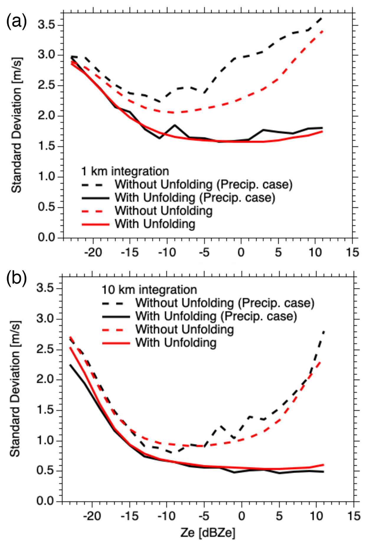
Figure 3 Standard deviation of the random error of simulated Doppler velocities for the PRF of the high mode (lower PRF) as a function of Z_e for (a) 1 km integration and (b) 10 km integration. The solid lines denote the results with unfolding correction. The black lines indicate the precipitation case in Hagihara et al. (2022).

Figure 4 illustrates the global mean SD of the random errors in the low-mode PRF. The dashed lines show SD_diff without unfolding correction and the solid lines indicate SD_diff with unfolding correction using Eq. (6). The PRF varies from 7156 to 7500 Hz, with a corresponding SD_random of 0.8 to 1.5 for 0 to −19 dBZ_e (see Fig. 2 in H22). On the other hand, in the high mode, the PRF varies from 6106 to 6464 Hz, with a corresponding SD_random of 1.5 to 3.4 for 0 to −19 dBZ_e. Similarly, V_max takes values between 5.7 and 6.0 m s⁻¹, whereas it is between 4.9 and 5.2 m s⁻¹ in the high mode. Comparison of Figs. 3 and 4 clearly shows that the SD of the random error is much smaller in the latter because of the SD_random described above. Furthermore, SD_diff without unfolding correction is smaller than that in the PRF of the high mode (lower PRF) because V_max is larger in addition to the effect of SD_random.

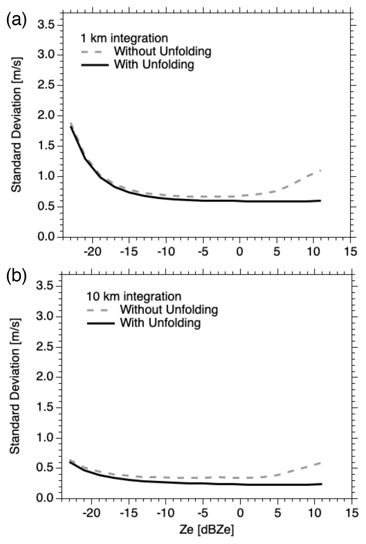
Figure 4 Standard deviation of the random error of simulated Doppler velocities for the PRF of the low mode (higher PRF) as a function of Z_e for (a) 1 km integration and (b) 10 km integration. The solid lines denote the results with unfolding correction.

As the frequencies of cloud and precipitation echoes differ in latitude and the PRF varies with latitude, as shown in Fig. 2, we investigated the change in SD_diff with latitude. We defined five latitudinal zones: the Arctic (> 60^∘), the northern midlatitude (60 to 30^∘), the tropics (30 to −30^∘), the southern midlatitude (−30 to −60^∘), and the Antarctic ($<-\mathrm{60}$^∘). In the following analysis, we focused on the SD_diff of V_10 km. Figure 5a–e show the SD of the random error for the five latitudinal zones in the PRF of the high mode (lower PRF). The dashed lines show the SD_diff without unfolding correction and the solid lines indicate the SD_diff with unfolding correction using Eq. (7). The SD_diff of V_10 km without unfolding correction decreases up to a certain value of Z_e and increases after that value. The SD_diff with unfolding correction decreases as Z_e increases. These tendencies observed in the five latitudinal zones are similar to those of the global mean SD_diff of V_10 km shown in Fig. 3b, although their magnitudes are not the same. We compared the SD_diff without unfolding correction. The SD_diff for the tropics, shown in Fig. 5c, has the largest value and is larger than the global mean result. The SD_diff values for both midlatitudes (Fig. 5b, d) are smaller than that for the tropics but slightly larger than or comparable to the global mean result. The SD_diff values for both polar regions (Fig. 5a, e) are even smaller than those for both midlatitudes and smaller than the global mean result. The SD_diff for the Antarctic in Fig. 5e shows the smallest value. The tendency of the magnitude relation of the SD_diff for each latitudinal zone was similar between cases without and with unfolding correction. From the PRF variation shown in Fig. 2, in the PRF of the high mode (lower PRF), the Doppler accuracy should be higher in the tropics and lower toward the poles. However, the results that we have seen so far show the opposite. On the other hand, the frequency of precipitation echoes is considered to be the highest in the tropics, and the folding Doppler error may have resulted in the largest SD_diff in the tropics. This does not mean, however, that the mean Doppler velocity of the precipitation echo exceeds V_max. In H22, Fig. 9a shows a 2D histogram of V_jsim without the random error as a function of the Z_e for the precipitation case. Large fall velocities are not seen due to Mie scattering of the larger drops at 94 GHz. As shown in Fig. 9b–d in H22, considering the random error due to the Doppler broadening, velocity folding occurs.

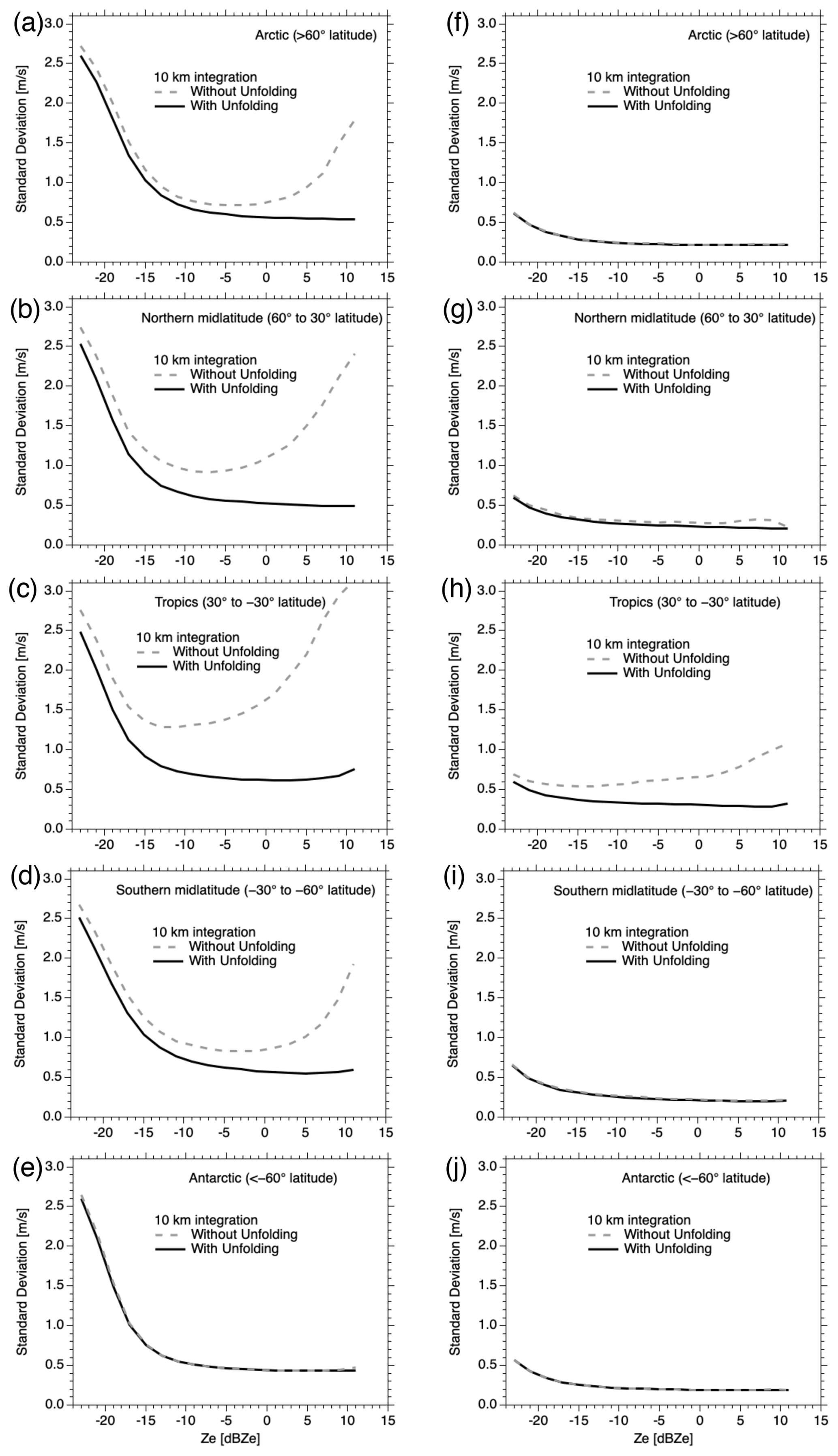
Figure 5 Standard deviation of the random error of simulated Doppler velocities for (a–e) the PRF of the high mode (lower PRF) and (f–i) the PRF of the low mode (higher PRF) as a function of Z_e after 10 km integration for (a, f) the Arctic, (b, g) the northern midlatitude, (c, h) the tropics, (d, i) the southern midlatitude, and (e, j) the Antarctic zones. The solid lines denote the results with unfolding correction.

Figure 5f–j demonstrate the SD of the random error for the five latitudinal zones in the PRF of the low mode (higher PRF). The dashed lines show the SD_diff without unfolding correction and the solid lines indicate the SD_diff with unfolding correction using Eq. (7). Similarly to Figs. 3 and 4, comparison of Fig. 5a–e and 5f–j shows that the SD_diff is much smaller in the latter. There is a difference between with and without unfolding correction only for SD_diff for the tropics (shown in Fig. 5h), although not for the others. This may be related to the frequency of precipitation echoes, as also explained in Fig. 5a–e. In the low-mode PRF, the V_max is larger and the SD_random is smaller owing to the higher PRF.

To summarize what has been discussed so far, the SD_diff values for the five latitudinal zones for 5 dBZ_e were extracted and are shown in Fig. 6. The red crosses indicate SD_diff without unfolding correction of the high-mode PRF, and the red circles denote the SD_diff with unfolding correction using Eq. (6). The dashed red line is the SD_diff for 5 dBZ_e without unfolding correction, and the solid red line is that with unfolding correction shown in Fig. 3b. The SD_diff without unfolding correction (red crosses) for the tropics is the largest at 2.2 m s⁻¹ and decreases in both polar directions, with the smallest value at 0.43 m s⁻¹ in the Antarctic. The SD_diff values for the northern midlatitude and the Arctic are slightly larger than those for the southern midlatitude and the Antarctic. In comparison with the global mean SD_diff without unfolding correction, the values for the tropics and northern midlatitude are larger, but the other values are smaller. The SD_diff with unfolding correction (red circles) for the tropics is 0.63 m s⁻¹, which is above the global mean result of 0.54 m s⁻¹ in Fig. 3b. The SD_diff values with unfolding correction for the southern midlatitude, northern midlatitude, and Arctic are comparable to the global mean result, but the value for the Antarctic is smaller than the global mean result. Next, we examine the PRF of the low-mode (higher-PRF) results. The blue crosses indicate the SD_diff without unfolding correction of the PRF of the low mode (higher PRF), and the blue circles denote the SD_diff with unfolding correction using Eq. (7). The dashed blue line is the SD_diff for 5 dBZ_e without unfolding correction, and the solid blue line is the value with unfolding correction illustrated in Fig. 4b. The SD_diff without unfolding correction (blue crosses) for the tropics is the largest at 0.78 m s⁻¹ and decreases toward the poles, with the smallest value being 0.19 m s⁻¹ in the Antarctic. The SD_diff with unfolding correction (blue circles) for the tropics is 0.29 m s⁻¹, which is above the global mean of 0.22 m s⁻¹ in Fig. 4b. The SD_diff values with unfolding correction for the other zones are comparable to the global mean result. As already explained in Fig. 5, the latitudinal variation in the SD_diff without unfolding correction may be due to the frequency of precipitation echoes. If the unfolding correction were perfect, there would be no relationship between the latitudinal variation in the SD_diff with unfolding correction and the frequency of precipitation echoes. However, there is actually a relationship between the two, which indicates a limitation of the unfolding correction.

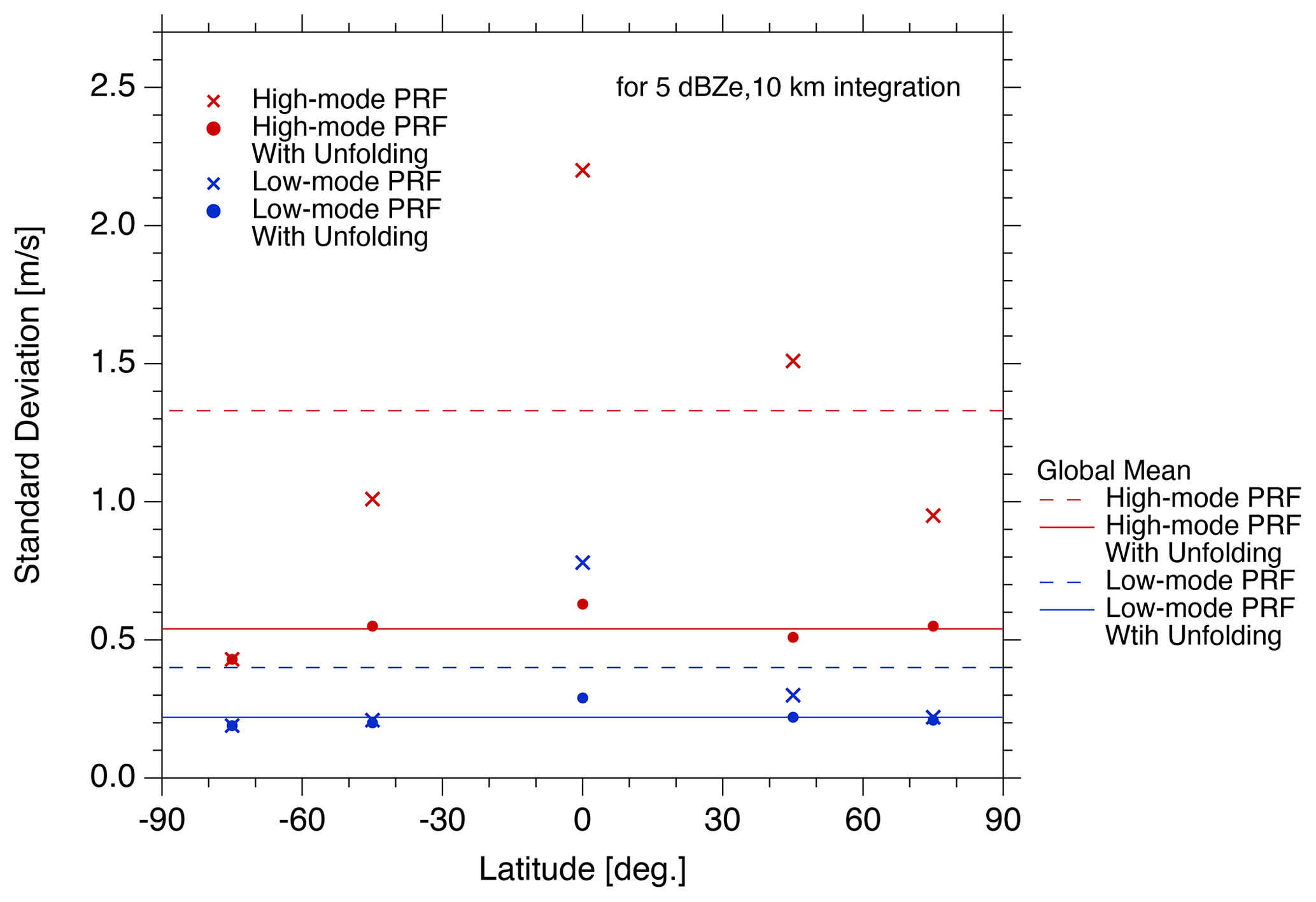
Figure 6 Standard deviation of the random error of Doppler velocities with and without unfolding correction for 5 dBZ_e after 10 km integration as a function of latitude.

We examined the zonal mean frequencies of precipitation echoes obtained from the NICAM/J-Sim data for 19 June 2008. First, to obtain precipitation echoes, we used the same method as in Fig. 1a but added a Doppler velocity condition (V_jsim>3 m s⁻¹, downward motion). Then, using the same bin size as in Fig. 1a, we obtained Fig. 7. The extracted precipitation echoes show that the frequency decreases at higher altitudes compared with that shown in Fig. 1a. The frequency is high in the tropics and decreases toward the poles. The frequencies at altitudes of less than 5 km were averaged by latitudinal zone and found to be as follows: 27.8 % in the Arctic, 60.3 % in the northern midlatitude, 68.5 % in the tropics, 36.7 % in the southern midlatitude, and 2.6 % in the Antarctic. This is because it was summer in the Northern Hemisphere in the simulation. The latitudinal variation in the SD_diff described so far can be explained on the basis of the precipitation echo distribution.

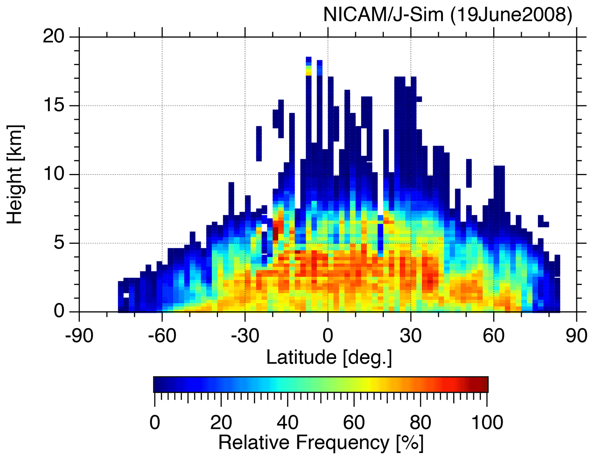
Figure 7 Zonal mean frequency of precipitation echoes obtained by NICAM/J-Sim for 19 June 2008.

4 Conclusions

We examined the vertical Doppler velocity error due to Doppler broadening and velocity folding in the EarthCARE CPR (EC-CPR) observations throughout the globe. We used simulated observation data (NICAM/J-Sim Z_e,jsim and V_jsim) for 16 satellite orbits with the same sampling interval as the EC-CPR, obtained using the NICAM and a satellite data simulator, the Joint-Simulator. The EC-CPR observed 500 m horizontally integrated pulse-pair covariances and Doppler velocity. The 1 and 10 km horizontally integrated Doppler velocities were calculated from them. We evaluated the Doppler error, i.e., the SD of the random error (SD_diff), and investigated the effectiveness of error reduction by horizontal integration. We also evaluated the Doppler folding error by comparing the corrected Doppler velocities using our simple unfolding method.

We first evaluated the global mean SD of the random error in the PRF of the high mode (lower PRF) as well as the PRF of the low mode (higher PRF) and compared the results with those of our previous study. In the PRF of the high mode (lower PRF), SD_diff without unfolding correction for 1 km integration decreases up to a certain value of Z_e and increases after that value. This decreasing feature is due to the decrease in the SD of the random error as the SNR increases, and the increasing feature is the result of an increase in the frequency of the folded Doppler error of precipitation echoes. The SD_diff without unfolding correction is much smaller for 10 km integration than for 1 km integration, because of the increased number of pulse pairs. When the unfolding correction is applied, the SD_diff becomes considerably smaller regardless of the integration length and the PRF mode. The results of the PRF of the low mode (higher PRF) show the very small SD of the random error both without and with unfolding correction.

To investigate the latitudinal variation in the SD of the random error, we separated the data into five latitudinal zones: the Arctic (> 60^∘), the northern midlatitude (60–30^∘), the tropics (30 to −30^∘), the southern midlatitude (−30 to −60^∘), and the Antarctic ($<-\mathrm{60}$^∘). In the present work, we focused on the SD_diff for 10 km integration. In the PRF of the high mode (lower PRF), the SD_diff for the tropics without unfolding correction is the largest and is larger than the global mean result. The SD_diff without unfolding correction decreases toward the poles with the smallest value for the Antarctic, which is smaller than the global mean. The tendency of the magnitude relation of the SD_diff for each latitudinal zone was similar between without and with unfolding correction. The frequency of precipitation echoes is expected to be highest in the tropics, and the folding Doppler error is also likely to be the largest. Therefore, the SD_diff for the tropics without unfolding correction is considered to be the largest. The SD_diff is much smaller in the PRF of the low mode (higher PRF) than in the PRF of the high mode (lower PRF), as shown by the global mean results described earlier.

In summary, the SD_diff for the five latitudinal zones for 5 dBZ_e is described as follows. In the PRF of the high mode (lower PRF), the SD_diff without unfolding correction for the tropics reached a maximum of 2.2 m s⁻¹ and then decreased toward the poles. The SD_diff with unfolding correction for the tropics was much smaller at 0.63 m s⁻¹. In the PRF of the low mode (higher PRF), the SD_diff without unfolding correction for the tropics reached a maximum of 0.78 m s⁻¹ and then decreased toward the poles. The SD_diff with unfolding correction for the tropics was 0.29 m s⁻¹, which is less than half the value without correction. As explained previously, the latitudinal variation in the SD_diff can be attributed to the frequency of precipitation echoes. The zonal mean frequency of precipitation echoes obtained from the NICAM/J-Sim data was higher in the tropics and decreased toward the poles. Therefore, the latitudinal variation in the the SD_diff can be explained on the basis of the precipitation echo distribution.

We found that the SD of the random error was higher in the tropics than in the other latitudes. In the tropics, the unfolding correction reduced the large SD of the random error more efficiently. However, the unfolding correction is also limited with respect to discrimination between large upward velocity and large precipitation falling velocity. Comparison of the results of the low mode and the PRF of the high-mode (lower-PRF) settings showed that the SD of the random error for the PRF of the low-mode (higher-PRF) setting was significantly reduced, although cloud echoes for altitudes higher than 16 km cannot be observed.