Validation of a camera-based intra-hour irradiance nowcasting model using synthetic cloud data

This work introduces a model for all-sky-image-based cloud and direct irradiance nowcasting (MACIN), which predicts direct normal irradiance (DNI) for solar energy applications based on hemispheric sky images from two all-sky imagers (ASIs). With a synthetic setup based on simulated cloud scenes, the model and its components are validated in depth. We train a convolutional neural network on real ASI images to identify clouds. Cloud masks are generated for the synthetic ASI images with this network. Cloud height and motion are derived using sparse matching. In contrast to other studies, all derived cloud information, from both ASIs and multiple time steps, is combined into an optimal model state using techniques from data assimilation. This state is advected to predict future cloud positions and compute DNI for lead times of up to 20 min. For the cloud masks derived from the ASI images, we found a pixel accuracy of 94.66 % compared to the references available in the synthetic setup. The relative error of derived cloud-base heights is 4 % and cloud motion error is in the range of $\pm \mathrm{0.1}\mathrm{m}{\mathrm{s}}^{-\mathrm{1}}$. For the DNI nowcasts, we found an improvement over persistence for lead times larger than 1 min. Using the synthetic setup, we computed a DNI reference for a point and also an area of 500 m×500 m. Errors for area nowcasts as required, e.g., for photovoltaic plants, are smaller compared with errors for point nowcasts. Overall, the novel ASI nowcasting model and its components proved to work within the synthetic setup.

1 Introduction

Clouds are a major modulator of atmospheric radiative transfer, as showcased by their ability to shadow the ground. This influence on the irradiance impacts the production of renewable energy through photovoltaic (PV) and concentrating solar power (CSP) plants. These fluctuations in produced power are a limitation for the usability of PV power. Unexpected variations in power production pose a challenge with respect to integration into power grids (Katiraei and Agüero, 2011). Prior knowledge of upcoming fluctuations and, therefore, short-term irradiance prediction can help mitigate this drawback of PV power production (e.g., West et al., 2014; Boudreault et al., 2018; Law et al., 2016; Chen et al., 2022; Samu et al., 2021; Saleh et al., 2018).

As direct irradiance can be blocked completely by clouds within seconds to minutes, knowledge of future direct irradiance is especially important for solar energy applications. Diffuse irradiance depends on complex 3D radiative transfer through the atmosphere. Variations in irradiance on the ground are relevant for solar energy applications – mainly due to variations in direct irradiance (Chow et al., 2011). Therefore, this study is focused on direct irradiance. Nowcasting of diffuse and global irradiance is not addressed.

Multiple models for intra-hour direct normal irradiance (DNI) nowcasting have been developed to predict the variability in direct irradiance. Many of these rely on so-called all-sky imagers (ASIs), ground-based cameras that capture hemispheric sky images (e.g., Chow et al., 2011; Peng et al., 2015; Schmidt et al., 2016; Kazantzidis et al., 2017; Nouri et al., 2022). The general idea is to extract cloud information from these images, predict future cloud positions, and accordingly estimate irradiance for the next minutes. The applicability of low-cost consumer-grade cameras makes setups with multiple ASIs financially feasible, and the increasing sizes of installed PV plants also require more measurement positions to expand nowcast areas. The Eye2Sky (Blum et al., 2021) network showcases the widespread use of multiple ASIs for regional coverage and nowcasting.

Common tasks for ASI-based DNI nowcasting are the extraction of cloud position and motion. Li et al. (2011) established a method to classify pixels based on color values and thresholds. A library of reference clear-sky images was introduced to extend this method and consider different atmospheric conditions and background variations for the large field of view (FOV) of ASIs (Shields et al., 2009; Chow et al., 2011; Schmidt et al., 2016). Furthermore, convolutional neural networks (CNNs) have been proven to work beneficially for these tasks (Ye et al., 2017; Dev et al., 2019; Xie et al., 2020; Hasenbalg et al., 2020) when trained on densely labeled data. Fabel et al. (2022) demonstrated the use of a CNN to distinguish not only clear and cloudy pixels but also further separate clouds into three subclasses: low-, mid-, and high-layer clouds. Moreover, Blum et al. (2022) projected cloud masks of multiple imagers onto a common plane and combined them for an analysis of spatial variations in irradiances. Masuda et al. (2019) combined a camera model with synthetic images of large-eddy simulation (LES) cloud fields to derive fields of cloud optical depth from images instead of simple cloud masks.

Setups with multiple ASIs allow for the estimation of cloud-base height using stereography (Nguyen and Kleissl, 2014; Beekmans et al., 2016; Kuhn et al., 2018b). Nouri et al. (2018) used four ASIs to derive height information and even a 3D cloud representation for irradiance nowcasting. Three ASIs were used by Rodríguez-Benítez et al. (2021) for three independent DNI nowcasts, which were finally averaged into a mean DNI nowcast.

Whilst measurements of irradiance through pyranometers are point measurements, nowcasting methods are usually targeted at solar power plants and, therefore, receiver areas. Kuhn et al. (2017a) derived area irradiance values using a camera monitoring shadows on the ground in combination with point irradiance measurements. ASI nowcasts for areas were found to outperform persistence for situations with high irradiance variability (Kuhn et al., 2017b). Nouri et al. (2022) computed ASI nowcasts for eight pyranometer measurement sites distributed over roughly 1 km². This study found reduced errors if nowcasts and measurements were averaged over all sites before error calculation in comparison with errors of individual point nowcasts.

Apart from application to real-world images, Kurtz et al. (2017) applied a DNI nowcasting model to synthetic ASI images of cloud scenes from LES models. The images were generated using a 3D radiative transfer model. This synthetic application comes with the advantage of optimal knowledge of the atmospheric state and allows for extended evaluation. The study showcased the problems introduced by the viewing geometry of ASIs.

In this study, we introduce a novel model for all-sky-image-based cloud and direct irradiance nowcasting (MACIN) and use synthetic data to validate it. This DNI nowcasting model is based on a setup with two ASIs. We use state-of-the-art techniques, e.g., to derive cloud masks using a CNN that was trained on sparsely labeled data. Cloud-base height (CBH) is derived by stereography and cloud motion by sparse matching. The derived cloud information is fed into a horizontal model grid using a method inspired by data assimilation. The method has similarities to the cloud mask combination of Blum et al. (2022) but allows the use of images from multiple time steps and is employed for nowcasting future states and not just analyzing the current situation. Predicted cloudiness states are projected to the ground and converted into DNI. We apply the techniques to synthetic ASI images generated from simulated LES cloud fields. This allows us to validate the derived quantities as well as the overall nowcast performance. Moreover, this allows for in-depth validation of DNI nowcasts, not just for single point measurements but also for areas, which is important for PV and CSP plants. Section 2 describes the synthetic data used throughout the study, the methods to derive information from ASI images, and the MACIN nowcasting model. The quantities and metrics used for validation are explained in this section as well. Section 3 describes the validation of derived cloud masks, cloud-base height, cloud motion, and the full DNI nowcasting model. Results of the validation are analyzed and discussed to affirm the presented methods and explain error sources. Conclusions can be found in Sect. 4 as well as a brief description of possible follow-up work.

2 Methods

The methods and data are described in this section. This includes an explanation of the synthetic data and all-sky images as well as the methods used to derive information about clouds in Sect. 2.1. The DNI nowcasting model that utilizes this information is outlined in Sect. 2.2. Reference quantities and metrics for validation are given in Sect. 2.3.

2.1 Synthetic data and all-sky images

The synthetic data were prepared by Jakub and Gregor (2022). This dataset is a 6 h LES run computed with the University of California Large-Eddy Simulation (UCLALES) model (Stevens et al., 2005). The horizontal resolution is 25 m, and LES output fields are given every 10 s. The initial atmospheric profile was chosen to produce a single shallow convection cloud layer with a cloud-base height of roughly 1000 m developing from a cloud fraction of 0 % in the beginning to roughly 100 % at the end of the simulation after 6 h. The reader is referred to Jakub and Gregor (2022) for more details and impressions of the cloud scenes used in this study.

This dataset provides realistic cloud situations and allows for detailed benchmarking. Cloud liquid water content (lwc) is the most important variable of the dataset for this study. To calculate the optical properties of clouds, the effective radius is also needed. As the LES output field does not contain this information, a fixed cloud droplet number density of $\mathrm{120}\times {\mathrm{10}}^{\mathrm{6}}{\mathrm{m}}^{-\mathrm{3}}$ was assumed. The effective radius of cloud droplets was calculated following Bugliaro et al. (2011). For simplicity, other atmospheric parameters like water vapor, temperature, pressure, and molecular composition from the LES output are neglected within this study, and the US Standard Atmosphere (Anderson et al., 1986) is assumed. While these atmospheric parameters and their variations are generally not negligible for radiative transfer, the setup for this study was simplified to focus on clouds as a major modulator of irradiance. Within this study, the Sun was assumed to be at a constant zenith angle of 30^∘ to the south.

We assume a fish-eye camera model corresponding to the OpenCV fish-eye camera model (Bradski, 2000) for synthetic images generated from these LES cloud fields. The parameters for this projection model were derived from the calibration of a CMS Schreder ASI-16 camera. This ASI features an 180^∘ FOV fish-eye objective to capture hemispheric images of the cloud situation. This study employs two distinct approaches to generating all-sky images from LES cloud scenes. We generate images with the viewing geometry derived according to the fish-eye camera model for the ASI-16 camera. As our methods are developed to work with cameras that are not necessarily calibrated spectrally, the images are only roughly optimized to resemble the colors of the ASI-16. We use a simple spectral camera model with white balance, black level, gamma correction, and an upper intensity limit to convert radiances into pixel values.

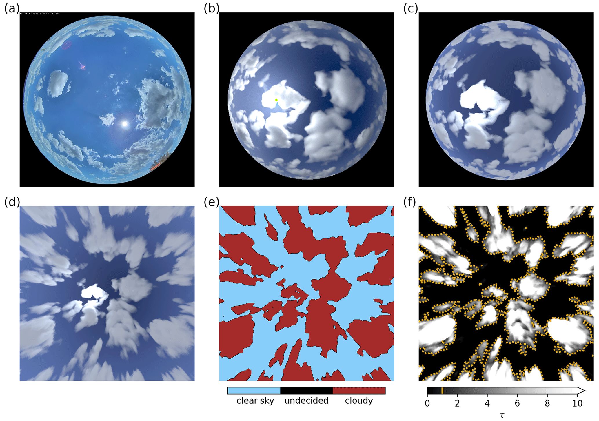
Figure 1 (a) Real ASI image captured with a CMS Schreder ASI-16 in the Bavarian countryside (48^∘10${}^{\prime }{\mathrm{50.3}}^{\prime \prime }$ N, 11^∘00${}^{\prime }{\mathrm{27.4}}^{\prime \prime }$ E) on 14 July 2020. (b–d) Synthetic images for an LES time of 9900 s generated using (b) MYSTIC, (c) ray-marching, and (d) ray-marching followed by projection. (e) Cloud mask derived from the projected ray-marching image and (f) LES cloud optical depth τ in the line of sight with the additional yellow contours illustrating τ_thresh=1.0. Only a few pixels are labeled “undecided” by the CNN, as depicted in panel (e).

One of the image generation methods uses synthetic radiances from the Monte Carlo 3D radiative transfer model MYSTIC (Mayer, 2009), which does not introduce any simplifying assumptions in radiative transfer. These radiances can be converted into synthetic images using the camera model. While MYSTIC radiances are physically correct, they are computationally expensive. Computation of these radiances for a single image requires multiple CPU hours; therefore, this approach was only used for 29 images with a resolution of 240 pixels × 240 pixels. In contrast, our second approach is only a rough approximation of radiative transfer. We use a ray-marching technology commonly applied in the computer gaming industry (e.g.,  Schneider, 2018; Hillaire, 2016) to trace through volumetric media. Many small steps along the line of sight are marched through the atmosphere for every pixel. At every step, light scattered into the line of sight of the simulated imager is computed using the local optical properties of the atmosphere. This is summed up to compute the overall light reaching the simulated imager. Schneider (2018) computed the direct radiation from the Sun at each step to estimate the amount of light scattered into the line of sight of the imager. Multiple scattering is only roughly parameterized in this approach, although it may be dominant in regions of high cloud optical thickness. Therefore, we use the original marching as well as a different method to calculate the amount of in-scattered light. Direct and diffuse irradiances are calculated with a two-stream radiative transfer model (Kylling et al., 1995) on tilted independent columns of the LES cloud field. For each ray-marching step, local irradiances are used to estimate the amount of direct and diffuse light scattered towards the simulated imager. This technique is implemented using the OpenGL framework and allows us to generate 960 pixel × 960 pixel images within seconds. Generated images are interpolated to the original ASI resolution in a post-processing step for both generation methods. Figure 1a–c show a real-world image as well as images generated using MYSTIC and ray-marching. Because of the low computational cost of image generation, we work with ray-marching images throughout this work if not stated otherwise. We derived cloud masks from both MYSTIC and ray-marching images to confirm the usability of the latter for our purpose.

As a first step in working with generated images, the camera model is applied to project them onto a horizontal, ground-parallel image plane. During reprojection, image features may be distorted and blurred. However, reprojection allows one to work on an image that is plane parallel to the ground, simplifying further image processing. Figure 1c and d display an image as captured by the ASI and its projected correspondence as generated using ray-marching. While the original ASI resolution is 1920 pixels × 1920 pixels, we project images to 480 pixels × 480 pixels for use within our nowcasting model.

2.1.1 Cloud masks

The most important information to obtain from all-sky images is the classification of pixels as cloudy or clear. Convolutional neural networks (CNNs), which are commonly applied for image segmentation, have also been applied to images of clouds to generate cloud masks (e.g., Dev et al., 2019; Xie et al., 2020; Fabel et al., 2022). Our cloud mask derivation relies on CNNs as well. We used the DeeplabV3+ network structure (Chen et al., 2018). The setup and training of the CNN are outlined briefly in the following, and a more detailed explanation can be found in Sect. A1 in the Appendix along with a description of the hand-labeling process of training data. Real-world images from an ASI-16 were chosen for this training dataset to avoid overfitting to generated ASI images of the limited LES dataset and to allow for easy future application of MACIN to real-world setups. Note that this is the only real measurement used throughout this study, and measurements otherwise refer to generated ASI images and simulated DNI. Training was done using 793 hand-labeled projected images depicting various cloud situations. Segmentation classes are “cloudy”, “clear”, and “undecided”. As the definition of cloudy and clear areas in images is often hard even for human observers, the CNN training is designed to ignore undecided image regions. The CNN is set up to reproduce the regions labeled as cloudy and clear, but it is free to fill in regions labeled as undecided by hand without impacting the training. Thus, the CNN fills in regions for which the cloud state is ambiguous or indistinguishable for humans based on its training on obvious cloudy and clear regions. From the CNN, we obtain cloud masks as a segmentation of an ASI image into the cloudy, undecided, and clear classes with respective scalar values of 1.0, 0.5, and 0.0. Figure 1d and e give a synthetic image and the derived cloud mask. For comparison, the LES cloud optical depth (τ) traced in the line of sight for each pixel is given in Fig. 1f.

2.1.2 Cloud-base height from stereo matching

In order to map cloud masks to 3D coordinates, cloud-base height (CBH) is required. For the experiments presented here, two ASIs are located within a 500 m north–south distance. Thus, for each time step, two viewing angles can be exploited to derive the CBH. Features from simultaneous ASI images of the same cloud scene are sparsely matched using efficient coarse to fine PatchMatch (CPM; Hu et al., 2016), a pixel-based pyramidal matching method. For a grid of pixels on the first input images, DAISY feature descriptors (Tola et al., 2010) are computed, and their best-matching counterparts in the second image are determined. As a result, we obtain a list of matched pixels from both images, which are supposed to depict the same part of a cloud. We use the derived cloud masks to filter matched pixels; valid matched pixels must be marked as cloudy in the corresponding cloud masks for both images to be accepted. Using the known camera geometry, a cloud-base height can be derived for each matched pair of pixels with the mispointing method developed by Kölling et al. (2019). This results in up to several thousand feature positions per pair of simultaneously captured images, which theoretically allows for a fine-grained treatment of the CBH. However, the nowcasting model presented in this study currently assumes a single cloud layer. Therefore, an image-wide average CBH is derived from the mean height of the feature positions.

2.1.3 Cloud motion

Cloud motion needs to be derived to predict future shading by clouds. Using the CPM matching algorithm on consecutive images taken in intervals of 60 s, we obtain matches describing the displacement of features. Computed cloud masks are used again to exclude matches lying outside of detected cloud areas. Average image cloud-base height and camera model are used to scale detected pixel movement to physical velocities within the assumed plane of clouds. A dense cloud motion field is obtained by nearest-neighbor interpolation of these sparse velocities.

2.2 Nowcasting model

The nowcasting model presented in the following uses derived cloud masks, the CBH, and cloud motion to predict future cloud situations and corresponding irradiance estimates. Cloud masks and cloud motion are represented as variables on a horizontal 2D grid, which will be referred to as cloudiness state and velocities. The 2D grid and all input data are assumed to be on one horizontal, ground-parallel level at the height given by the derived CBH. Multi-level clouds are not yet represented as such by our model. Future states of these 2D fields are predicted using a simple advection scheme. Irradiance estimates are computed from these future cloudiness states. All derived cloud masks and cloud motions are combined into an optimized initial state of the horizontal 2D fields. The nowcasting model therefore consists of three major parts: a simple advection method, a method inspired by data assimilation to determine the initial state, and a radiative transfer parametrization to calculate DNI from the cloudiness state. These three parts are explained more closely in the following.

2.2.1 Advection scheme

The nowcasting model is based on a 2D grid with a grid spacing of $\mathrm{\Delta }x=\mathrm{\Delta }y=\mathrm{10}\mathrm{m}$ and a number of grid points $N=M=\mathrm{1600}$ in the x and y directions, respectively, thereby covering 16 km×16 km. Variables on each grid point are cloudiness state (cm) and cloud velocities (u and v) in the x and y directions, respectively. Starting from an initial state at the first iteration t₀=0 s and a temporal resolution of Δt=60 s, future cloudiness states at times $t_i=t_{\mathrm{0}}+i\cdot \mathrm{\Delta }t$ are computed using advection as follows:

$$\begin{array}{}\text{(1)}& {\displaystyle }& {\displaystyle }{\mathrm{cm}}_{t_{i+\mathrm{1}}}(n,m)={\mathrm{cm}}_{t_i}\left(\stackrel{\mathrm{̃}}{n},\stackrel{\mathrm{̃}}{m}\right),\text{(2)}& {\displaystyle }& {\displaystyle }\stackrel{\mathrm{̃}}{n}=n-\mathrm{int}\left(\mathit{\lambda }\cdot u(n,m)\right),\text{(3)}& {\displaystyle }& {\displaystyle }\stackrel{\mathrm{̃}}{m}=m-\mathrm{int}\left(\mathit{\lambda }\cdot v(n,m)\right),\end{array}$$

where $\mathit{\lambda }=\mathrm{\Delta }t/\mathrm{\Delta }x$. The coordinates $(\stackrel{\mathrm{̃}}{n},\stackrel{\mathrm{̃}}{m})$ determined by advection using physical velocities are restricted to discrete grid coordinates and, therefore, integers. This constrains actually representable velocities to multiples of $\mathrm{\Delta }x/\mathrm{\Delta }t$. Continuous boundary conditions are assumed. The same advection scheme is applied to the horizontal velocities fields u_t(n,m) and v_t(n,m) as well.

2.2.2 Data assimilation

The cloud mask and horizontal velocity field from one imager and time step as well as an estimation of cloud-base height would be sufficient to initialize the advection model. However, for each nowcast, we do have cloud masks and velocities from two imagers with different viewing geometries and multiple time steps. In order to make use of as much information as possible for the initial state, we employ a method similar to 4D-Var data assimilation (Le Dimet and Talagrand, 1986) in numerical weather prediction models. The general idea is to define a scalar function of an initial model state that measures differences between model states and measurements. This so-called cost function is then iteratively minimized to find an optimal model state for given measurements. We reference “measurements” in this section and the following. We thereby mean the synthetic generated ASI images and simulated DNI values, not real measurements.

The difference between model state and measurements needs to be assessed at matching times. Model states for multiple time steps are therefore computed from the initial state at time t₀ using the previously described advection M. Model cloudiness states at time t_k will be denoted as $\mathrm{cm}\left(t_k\right)=M(\mathrm{cm},t_k)$ with initial cloudiness state cm. Horizontal velocities u and v are described analogously. We define the cost function J for L time steps in the interval [t₀,t_l] and two ASIs ($p\in \mathrm{1},\mathrm{2}$) as follows:

$$\begin{array}{}\text{(4)}& \begin{array}{rl}& J(\mathrm{cm},u,v)=\sum _{N,M}\sum _{l=\mathrm{0}}^L\sum _{p=\mathrm{1}}^{\mathrm{2}}\left({\displaystyle \frac{\mathrm{1}}{{\mathit{\sigma }}_{\mathrm{cm}}}}\cdot \left(\mathrm{cm}\left(t_l\right)\right.\right.\\ & {\left.-{\mathrm{cm}}_{\mathrm{meas},l,p}\right)}^{\mathrm{2}}+{\displaystyle \frac{\mathrm{1}}{{\mathit{\sigma }}_{uv}}}\cdot {\left(u\left(t_l\right)-u_{\mathrm{meas},l,p}\right)}^{\mathrm{2}}\\ & +\left.{\displaystyle \frac{\mathrm{1}}{{\mathit{\sigma }}_{uv}}}\cdot {\left(v\left(t_l\right)-v_{\mathrm{meas},l,p}\right)}^{\mathrm{2}}\right)+R(u,v),\end{array}\end{array}$$

with measurements of cloud masks ${\mathrm{cm}}_{\mathrm{meas},l,p}$ and horizontal velocities at time step l from imager p interpolated to the model grid. Summation over all grid points is indicated by ${\sum }_{N,M}$ for better readability. The coefficients σ_cm=0.1 and ${\mathit{\sigma }}_{uv}=\mathrm{10.0}\mathrm{m}{\mathrm{s}}^{-\mathrm{1}}$ are supposed to account for uncertainties in the respective measurements but are mainly used as tuning parameters here. More complex, non-scalar coefficients could differentiate, for example, between varying measurement quality within ASI images or between different imagers, but they require characterization of the system, which is usually not available. The additional regularization term denoted as R(u,v) is used to suppress measurement errors, especially outliers in the velocity field. In detail, it is

$$\begin{array}{}\text{(5)}& R_{uv}(u,v)={\mathit{\sigma }}_{R,uv}\cdot \left({\left(\mathrm{\nabla }u\right)}^{\mathrm{2}}+{\left(\mathrm{\nabla }v\right)}^{\mathrm{2}}\right),\end{array}$$

with tuning parameter ${\mathit{\sigma }}_{R,uv}=\mathrm{250}{\mathrm{s}}^{-\mathrm{1}}$ chosen to smooth the velocity field. As cloud masks are especially hard to derive from ASI images in the bright region of the Sun, measurement values are excluded from the assimilation if they are derived from an image region of 2.5^∘ around the Sun. Erroneous cloud mask values derived for the bright Sun and zero velocities derived from the static Sun position are thereby avoided. Figure 2 illustrates the measurements, first guess, and analysis state after assimilation for an example assimilation run. Due to the limited complexity of the advection scheme and the high-resolution observations from images, a background state is not used. Model states of previous nowcast runs are not used within assimilation. This means that successive nowcast runs are independent, as states from previous model runs for the nowcast start time are not considered in additional terms in Eq. (4). Average cloudiness state and velocities from all measurements available at the time of the initial state are used as a first guess for cost function minimization. The cost function is minimized using the bounded L-BFGS-B algorithm (Zhu et al., 1997). For efficient optimization, the advection model and cost function were implemented using the PyTorch framework (Paszke et al., 2019), which allows for automatic calculation of the adjoint of the cost function. The optimized model state is finally used for the actual nowcast as the initial state of the advection model.

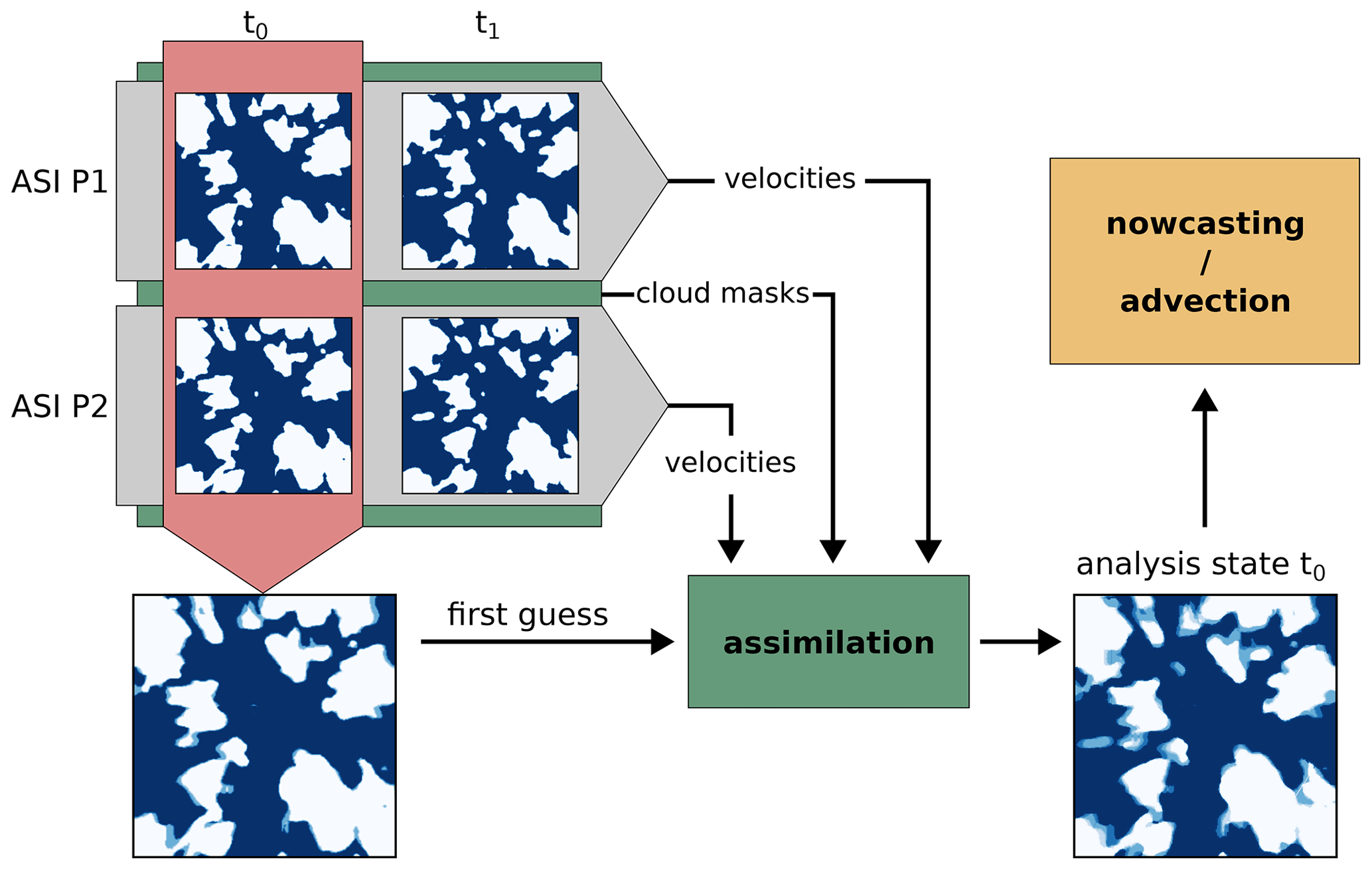
Figure 2 Illustration of cloud mask measurements, the derived first guess used for assimilation, and the analysis state found by assimilation for an LES time t₀=8940 s. Shown is the cloudiness state and the inner 8 km×8 km of the domain. The analysis state is less sharp on cloud edges due to the consideration of multiple cloud mask measurements.

2.2.3 Radiative transfer parametrization

Direct solar irradiance is reduced by interaction with molecules, aerosol, and clouds. For this study, we assume that short-term changes in direct irradiance are mainly caused by clouds and neglect other variations. DNI is parameterized using previous irradiance measurements on site as well as predicted cloud masks. “Measurements” in the following do not describe real-world measurements with, for example, a pyranometer, but instead detail DNI values simulated for LES scenes. The idea of the parametrization is to derive references for occluded and non-occluded cases from measurements. Depending on the cloudiness state, the DNI is then interpolated from these references. Therefore, a time series of clear-sky index (CSI) values k is constructed from DNI measurements as the ratio of measurements and a simulated clear-sky DNI_clear. From this time series, values of k are extracted for two sub-series: occluded (k>0.9) and non-occluded (k<0.1) times. We define the occluded CSI k_occl and non-occluded CSI k_clear as the exponentially weighted mean with a half-life time of 10 min from respective measurement subsets. CSI values for a non-occluded and a fully occluded Sun are interpolated linearly. A sun disk of 0.5^∘ opening angle at the given Sun elevation and azimuth is projected onto the 2D model grid. The mean cloudiness state of all grid points in the sun disk (cm_sun) is used to calculate DNI for time t as follows:

$$\begin{array}{}\text{(6)}& \begin{array}{rl}\mathrm{DNI}\left(t\right)& ={\mathrm{DNI}}_{\mathrm{clear}}\cdot \left((\mathrm{1}-{\mathrm{cm}}_{\mathrm{sun}}(t\left)\right)\cdot k_{\mathrm{clear}}\right.\\ & \left.+{\mathrm{cm}}_{\mathrm{sun}}\left(t\right)\cdot k_{\mathrm{occl}}\right).\end{array}\end{array}$$

The exponentially weighted mean is used for the computation of k_occl and k_clear in order to smooth the latest fluctuations and provide a values for all times.

2.3 Synthetic data experiment setup

The synthetic setup allows us to compare quantities derived by the nowcasting model to synthetic reference values. Within this study, we simulate a setup around a fictional 500 m×500 m area PV power plant. As depicted in Fig. 3, all-sky images are generated for synthetic imagers at positions P1 and P2 centered on the northern and southern boundaries of this area. Direct normal irradiance values were calculated for point P1 and the full 500 m×500 m area A1 as explained later on. Images are rendered with MYSTIC and ray-marching, as explained in Sect. 2.1, for a synthetic ASI at P0 at the southeastern edge of A1 to compare both methods. Ray-marching images for P1 and P2 are used for actual nowcasting and all other applications in this study.

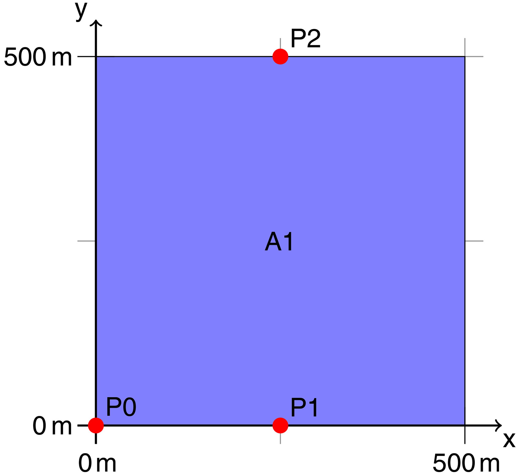
Figure 3 Spatial setup for the synthetic experiments conducted in this study. Shown are the ground coordinates within the LES domain. Synthetic all-sky images were generated at points P0, P1, and P2. Direct normal irradiance was simulated for point P1 and area A1. Nowcasts rely on images from P1 and P2 and predict values for point P1 and area A1.

Validation quantities used within the experiments in Sect. 3 are explained in the following. Cloud optical depth (τ) is traced in the line of sight for every pixel of the corresponding ASI image and used to validate derived cloud masks. By applying a threshold to the resulting τ fields, we can calculate reference cloud masks. Figure 1f shows an example τ field. These are used for the validation of the derived CNN cloud masks. The cloud-base height reference is computed in compliance with the view of an ASI. The last scattering of light before reaching the ASI sensor gives the origin of pixel information – in this case, cloud height as seen from below. MYSTIC can be used not only to compute radiances but also to obtain these scattering positions. A cloud motion reference is hard to define, as clouds in the LES simulation – as in nature – are not moving as solid objects but may change size and shape or even appear and disappear. Therefore, wind velocities at cloud level may not be an exact benchmark for the overall observable cloud motion. Within this study, we use the vertically integrated liquid water path (lwp) from the LES fields as an indicator of horizontal cloud distribution. The maximum cross-correlation between the domain-wide lwp of two successive time steps is assumed to be a reference for average cloud motion. This reference describes the mean displacement for all time steps of the LES cloud data. However, clouds are convectively reshaping, growing, and shrinking in these data, which makes this cloud motion definition vague. The synthetic data allow for a more direct validation of cloud motion. LES cloud fields can be frozen for a time step and their position shifted. This basically simulates scenes of pure advection without any convective effects. To simulate this advective case for cloud motion validation, we use two images of the same cloud scene but taken from different positions. The choice of an assumed time difference between the images Δt defines the advective cloud velocity. For simplicity, we use images taken within a 500 m north–south distance, as represented by P1 and P2. Assuming Δt=60 s, we obtain theoretical cloud velocities of $-\mathrm{8.3}\mathrm{m}{\mathrm{s}}^{-\mathrm{1}}$ meridionally and 0 m s⁻¹ zonally.

The Monte Carlo 3D radiative transfer solver MYSTIC was used to compute radiances for images and true direct normal irradiances at ground level. We calculated direct normal irradiance for two different synthetic references, as depicted in Fig. 3. A DNI point reference is simulated at P1, and an area reference of the 500 m×500 m region A1 is simulated with ASIs centered at the northern and southern boundaries at P1 and P2. As a benchmark for the DNI nowcasting model, persistence nowcasts for start time t₀ and nowcast time t are calculated from simulated DNI “measurements” at DNI_P1 as follows:

$$\begin{array}{}\text{(7)}& {\mathrm{DNI}}_{\mathrm{pers}}\left(t\right)={\mathrm{DNI}}_{\mathrm{meas}}\left(t_{\mathrm{0}}\right).\end{array}$$

The metrics used for validation are the root-mean-square error (RMSE), the normalized root-mean-square error (NRMSE), and the mean bias error (MBE):

$$\begin{array}{}\text{(8)}& \mathrm{RMSE}=\sqrt{{\displaystyle \frac{\mathrm{1}}{N}}\sum _{i=\mathrm{1}}^N{\left(x_i-x_{\mathrm{ref},i}\right)}^{\mathrm{2}}},\end{array}$$

$$\begin{array}{}\text{(9)}& \mathrm{NRMSE}=\sqrt{{\displaystyle \frac{\mathrm{1}}{N}}\sum _{i=\mathrm{1}}^N{\left({\displaystyle \frac{x_i-x_{\mathrm{ref},i}}{x_{\mathrm{ref},i}}}\right)}^{\mathrm{2}}},\end{array}$$

and

$$\begin{array}{}\text{(10)}& \mathrm{MBE}={\displaystyle \frac{\mathrm{1}}{N}}\sum _{i=\mathrm{1}}^N\left(x_i-x_{\mathrm{ref},i}\right),\end{array}$$

with the quantity to be evaluated x, its corresponding reference x_ref, and the number of values N. Additionally, we use the pixel accuracy

$$\begin{array}{}\text{(11)}& \mathrm{PA}={\displaystyle \frac{\mathrm{CCLD}+\mathrm{CCLR}}{N_{px}}}\end{array}$$

with the number of correctly classified cloudy or clear pixels (CCLD and CCLR, respectively) as well as the overall number of pixels (N_px).

3 Validation using synthetic data

3.1 Cloud masks

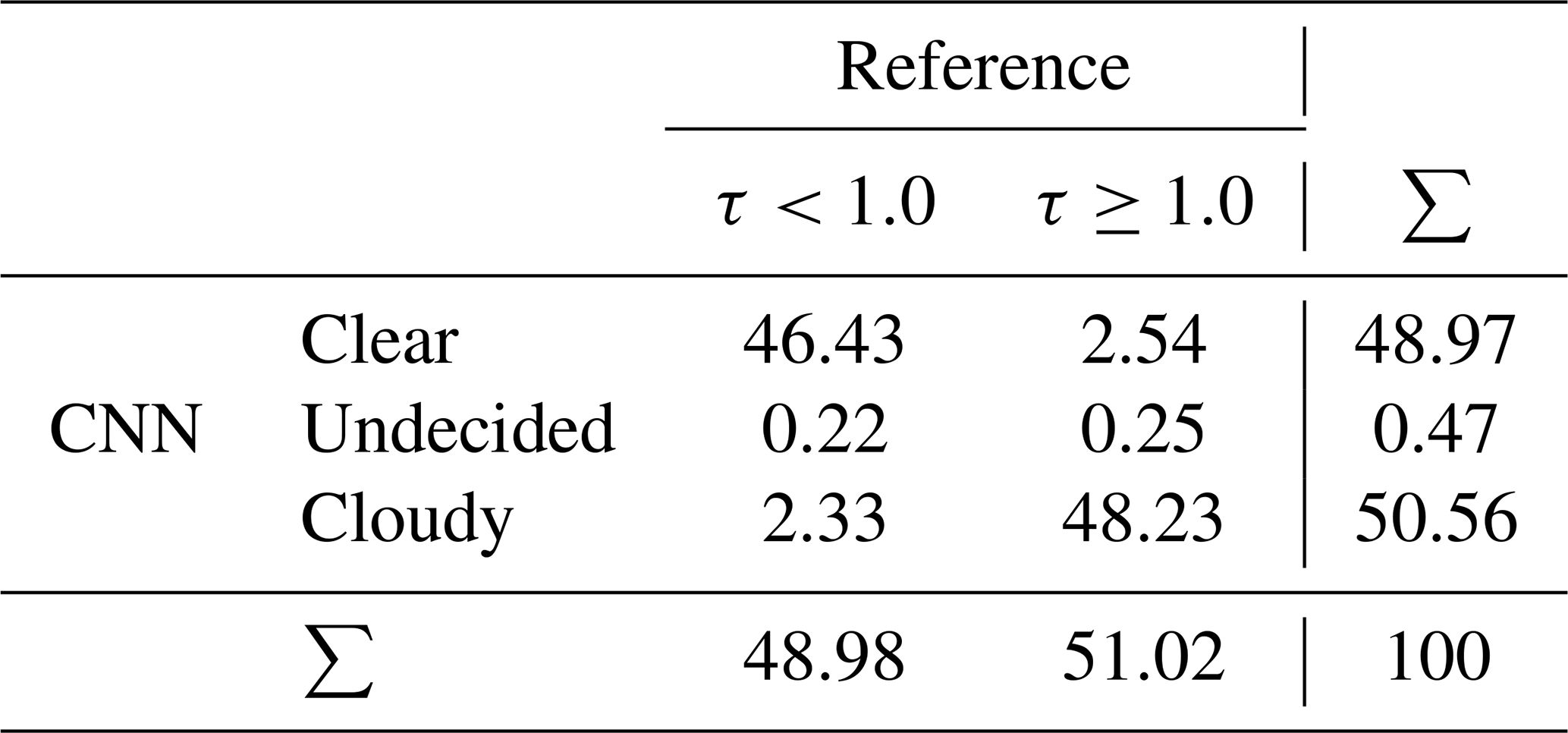
The CNN cloud mask model was successfully trained and validated on hand-labeled real-world images, as explained in Sect. A1 in the Appendix. We evaluate derived cloud masks to show that it is reasonable to apply the cloud mask CNN to the synthetic images in this study. We calculated the path cloud optical depth (τ) for all viewing angles of our ASI and every desired time step. Together with a threshold, this gives a reference cloud mask. To validate pixel-wise cloud classifications, we use a threshold of τ_thresh=1.0 to create reference cloud masks from τ. Values of τ≥τ_thresh are linked to cloudy areas in these τ_thresh cloud masks. We evaluated CNN cloud masks from ray-marching images for position P1 and 360 time steps at 60 s intervals covering all LES times. The contingency table (Table 1) displays the distribution of classes of τ_thresh cloud masks against our CNN cloud masks. In general, we find very good compliance. Each of the cloudy and clear classes makes up about 50 % of the compared pixels, which corresponds well to the τ_thresh cloud masks. Cloud masks of our CNN exhibit a slight bias towards classifying too few pixels as cloudy. Pixel accuracy is PA=94.66 % against the τ_thresh cloud masks.

Table 1 Contingency table for the cloud mask classes from the CNN and cloud optical depth τ in the line of sight thresholded given by τ_thresh=1 as a reference. All values are given as a percentage.

Beyond ray-marching images, we calculated 29 MYSTIC images and computed CNN cloud masks for these. By doing the same with corresponding ray-marching images, we could ensure that the derived cloud masks exhibit similar performance for both image generation approaches. As MYSTIC images are physically correct, we conclude that the usage of approximated ray-marching images does not affect the validity of our results.

3.2 Cloud-base height

We used data from for the entire LES scene and, effectively, 319 time steps with clouds for the validation of derived CBH. Ray-marching images taken at P1 and P2 were used to derive the CBH as in the nowcasting model. Computed scattering positions give the reference CBH. As our nowcasting model assumes a single cloud-base height, we average the derived CBH per image pair. Figure 4a shows the derived average CBH per image pair and the corresponding reference CBH. For these averaged heights, we obtain a MBE for the mispointing method of 50.7 m, an RMSE of 56.9 m, and a NRMSE of 4.0 %. When subtracting the found bias of 50.7 m from the derived image average cloud-base heights, the RMSE could be reduced to 25.6 m and NRMSE to 2.6 %. Increasing systematic error can be observed for the reference CBH up to about 1400 m. A histogram of all derived pixel heights, which are the basis for the averaged CBH, and their reference is shown in Fig. 4b. Similar to the image-wide average cloud-base height, derived pixel heights show good agreement with reference heights and a small systematic overestimation. Reference pixel heights show a wider distribution compared with derived values, resulting in the stripes visible in Fig. 4. Found height errors could result from discrete viewing directions due to the limited resolution of images, from the projection process, and from the discrete stepping of the image generation ray-marching algorithm. Error sources were not investigated further, as errors are in the range or even lower than those found in other studies with respect to derived cloud-base heights (e.g., Nguyen and Kleissl, 2014; Kuhn et al., 2019; Blum et al., 2021). Equally, no additional work was done to mitigate the observed systematic errors for use in nowcasting.

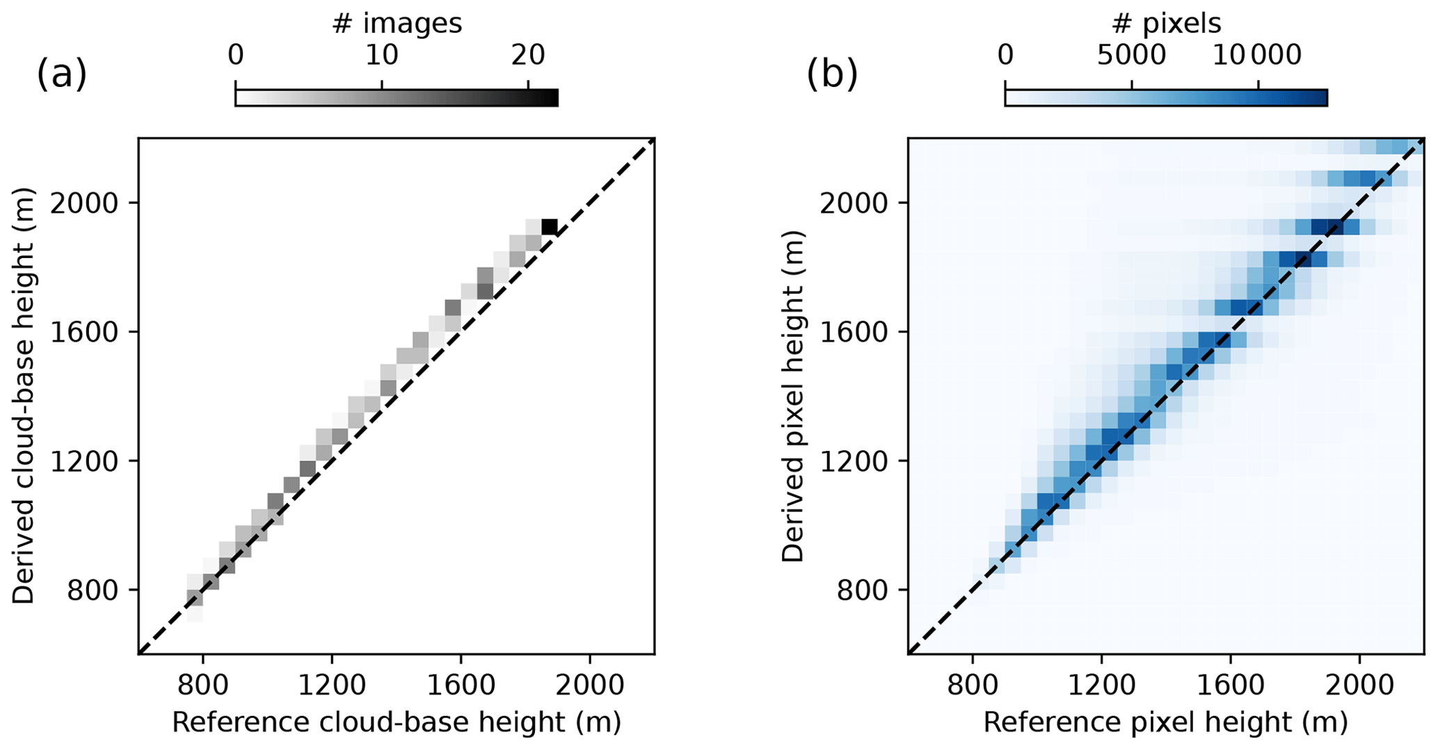
Figure 4 Histogram of (a) image mean cloud-base height and (b) height derived for the matched pixels of all images compared against synthetic references.

3.3 Cloud motion

As wind is not necessarily an exact benchmark for cloud motion in convective cloud scenes, we chose two ways to validate our derived cloud motion for two cases. Cloud motion according to the LES is used as a convective case where clouds also develop and decay. Additionally, we are interested in the performance when cloud motion is pure advection, i.e., only displacement of frozen cloud fields. This advective case allows one to derive an exact reference for cloud motion, and the convective case allows one to validate the quality of the derived cloud motion in the presence of clouds that change their size and shape.

Validation of cloud motion in the convective case is done on images every 60 s for LES times from 0 to 21540 s. Figure 5 shows cloud fraction as a function of LES time. The average displacement of the vertically integrated liquid water path (lwp) between time steps is calculated using maximum cross-correlation and used as a reference. This describes mean translation and is, therefore, a proxy for domain-averaged reference cloud motion. Cloud motion vectors derived by sparse matching are averaged per time step and ASI and are compared against this reference. Figure 5 shows zonal and meridional winds derived for both the ASI and the reference determined by lwp cross-correlation. The cloud fraction derived from cloud masks of an ASI at P1 is given as an indicator of the cloud situation. Up to an LES time of approximately 3600 s, no significant visually detectable clouds are present; therefore, no velocities are derived. Up to approximately 6000 s, derived velocities are relatively unstable over time, with changes in estimated velocities of up to 1.7 m s⁻¹ over 60 s. We relate this to the rapidly changing nature of small convective clouds in combination with a low cloud fraction. During this time, some of the small clouds appear and disappear in between time steps and are, therefore, mismatched. After approximately 6000 s, derived zonal velocities vary in a range of $\pm \mathrm{0.5}\mathrm{m}{\mathrm{s}}^{-\mathrm{1}}$ between time steps. Zonal cloud motion close to zero matches the LES initialization without zonal wind. Meridional velocities increase from about 3 m s⁻¹ at 6000 s to a maximum of 4.7 m s⁻¹. In general, our derived zonal velocities show a less noisy estimate compared with the reference. Derived velocities from both ASIs show very similar patterns. This further affirms the stability of the cloud motion derivation. However, we do not have an absolute reference to benchmark derived velocities in the convective case, as pure displacement of convective clouds is hard to capture and may differ strongly from main winds. We validate derived cloud velocities using artificially advected cloud fields to overcome this limitation. The same LES times as in the convective validation are used, but each time step is assumed to be independent. Cloud motion is generated by freezing the cloud field and shifting it for each time step. This results in an objective reference cloud motion. A shift of 500 m from north to south at a time difference of 60 s gives a theoretical u of 0 m s⁻¹ and v of $-\mathrm{8.3}\mathrm{m}{\mathrm{s}}^{-\mathrm{1}}$. No velocities were derived in the absence of clouds up to approximately 2500 s. Afterwards, the derived velocities match the theoretical displacements well with an RMSE of 0.019 m s⁻¹ zonally and 0.11 m s⁻¹ meridionally.

Overall, these results prove that the derived cloud motions are reliable for the cloud situations used in this study. This can also be seen as a further validation of derived CBHs, as they are necessary for the calculation of physical velocities.

Figure 5 (a) Cloud fraction from cloud masks of the ASI at P1 for LES times. Per time step scene-averaged cloud motion derived using cross-correlation of the lwp field of the LES simulation and our cloud motion derivation based on feature matching for east to west motion u (b) and south to north motion v (c).

3.4 DNI nowcasts

Evaluation of the nowcasting model is done using multiple steps that are described and discussed in the following. MACIN is compared against persistence to evaluate overall performance. Additionally, variations of MACIN using ideal cloud masks were run to investigate the implications of errors in CNN-derived cloud masks. These variation runs will be called “cloud mask variation” and “continuous cloud mask variation” hereafter and explained later on. Finally, a simplification of MACIN is used to assess possible benefits of the expensive assimilation of MACIN. This variation will be referred to as “simple variation”. For MACIN and all its variations, one nowcast run was started every 60 s for LES times from 60 to 21 540 s for a total of 359 nowcast runs. The maximum nowcast lead time was chosen as 20 min. Nowcast time steps exceeding the maximum LES time of 21 600 s were discarded. DNI nowcasts are always derived simultaneously for point P1 and area A1. Errors for point and area forecasts show similar characteristics. Therefore, they are discussed jointly in the following. If not stated otherwise, error values are given for the point DNI with the area DNI given in parentheses.

Figure 6a and b show the average RMSE and MBE for point nowcasts of persistence, MACIN, and cloud mask variation grouped by lead time. Figure 6c and d give the same for area nowcasts. Errors of persistence and MACIN give the overall performance of the introduced nowcasting model and are, therefore, analyzed first. Persistence nowcasts start without error at a lead time of 0 min, but the RMSE increases strongly up to approximately a constant value of 300 W m⁻² (250 W m⁻²) after 6 min. The persistence MBE increases linearly up to approximately 50 W m⁻² and is linked to the tendency of a growing cloud fraction over time. MACIN exhibits a nonzero RMSE at nowcast start but a smaller increase in the RMSE over time compared with persistence. In terms of the RMSE, MACIN outperforms persistence for lead times longer than 1min. Improvements over persistence for these longer lead times are thereby typically on the order of 50 W m⁻² (50 W m⁻²) or more. In general, the RMSE of nowcasts for areas is about 50 W m⁻² lower than nowcasts for points. The MBE is mostly negative for MACIN, with magnitudes in the range of the persistence MBE. The nonzero RMSE at a lead time of 0 min may be a result of erroneous cloud masks in the region of the Sun, errors in the radiative transfer (RT) parametrization, or smearing out during the assimilation because of multiple time steps and viewing geometries.

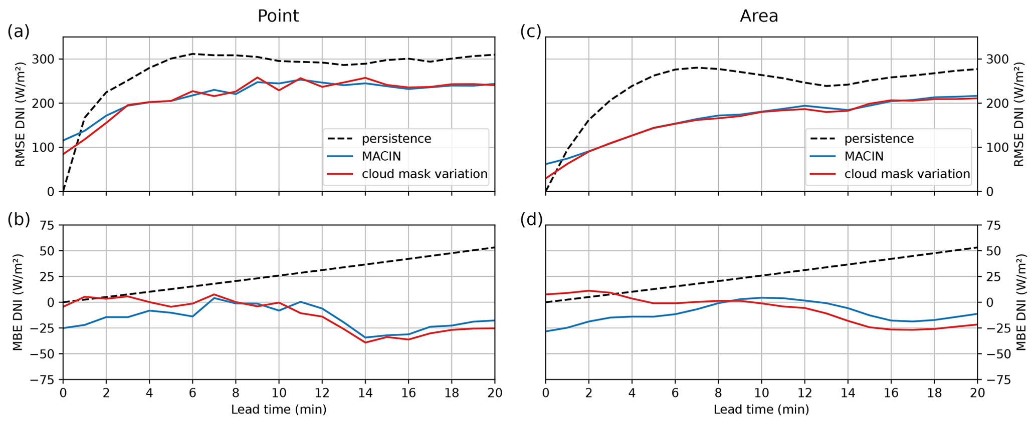
Figure 6 The (a) RMSE and (b) MBE for 359 point DNI nowcasts compared to DNI point reference values and evaluated per lead time. Nowcasts were done using MACIN and the cloud mask variation. Panels (c) and (d) show corresponding error values for the area nowcasts and DNI area reference.

To further investigate the initial nowcast error discussed above, a cloud mask variation of MACIN was run. Perfect cloud masks were used as input for the nowcasting model instead of CNN cloud masks. These perfect cloud masks are derived from the LES cloud optical depths in the line of sight τ (see also Sect. 3.1 and Fig. 1f) with a threshold of τ_thresh=1.0 to distinguish between cloudy and clear-sky conditions. By using these perfect cloud masks for nowcasting, the influence of cloud mask errors within the nowcasting model can be assessed. As for the persistence and MACIN, nowcast errors for the cloud mask variation are given in Fig. 6. The RMSE of the cloud mask variation is very similar to the RMSE of MACIN. This suggests that the CNN cloud masks provide a good estimate of the cloud situation for our nowcasting. However, the cloud mask variation outperforms MACIN by 31 W m⁻² (32 W m⁻²) for a lead time of 0 min and converges to the RMSE of MACIN for lead times of 3 min and longer. The cloud mask variation point MBE is initially about 0 W m⁻²; therefore, the negative MBE of MACIN, especially during the first minutes of the nowcasts, can be associated with erroneous cloud masks in the vicinity of the Sun. The minor improvement for longer lead times when using perfect cloud masks might also be a result of the convectively growing, shrinking, and reshaping clouds. As the nowcasting model cannot describe these processes, perfectly outlining clouds in the beginning may not be that relevant for longer lead times. The nonzero RMSE of the cloud mask variation for a lead time of 0 min may result from errors in the RT parametrization or smearing out by assimilation, as described for MACIN before. To further investigate the implications of the RT parametrization, the continuous cloud mask variation was run. It differs from MACIN only with respect to the input cloud masks. In contrast to the cloud mask variation, which gives discrete cloud mask values for clear-sky and cloudy classes, the continuous cloud mask variation relies on cloud masks with continuous values. The RT parametrization maps model cloudiness states linearly to DNI values. Model cloudiness states of MACIN usually rely on CNN cloud masks with discrete values for the three classes (clear, cloudy, and undecided), whereas actual cloud optical depth is a continuous variable. Continuous cloud masks are used to check whether this discrete representation causes a significant fraction of nowcast error. These cloud masks are derived from τ used for the cloud mask validation, but they comply with the exponential attenuation of intensity in radiative transfer by ${\mathrm{cm}}_{\mathrm{cont}}=\mathrm{1}-\exp \left(\mathit{\tau }\right)$. The continuous cloud mask variation uses these continuous cloud masks. The resulting errors of the continuous cloud mask variation are not depicted, as they strongly resemble the errors of the cloud mask variation with slight improvements in the RMSE in the range of about $\pm \mathrm{5}\mathrm{W}{\mathrm{m}}^{-\mathrm{2}}$. Therefore, we conclude that the RT parametrization and discrete nature of cloud masks is not a major error source, and the nonzero RMSE for a lead time of 0 min is a result of smearing out during assimilation.

A further variation of MACIN was run to assess the benefits of the assimilation scheme. Therefore, the simple variation of MACIN was run with just a single cloud mask and velocity field from the ASI at P1 as input. The Sun region is not masked out in the cloud mask and velocity field for the simple variation. With this variation, we assess the possible benefits of the additional complexity and computational cost of MACIN. The resulting errors differ from the errors of MACIN, mainly for point nowcasts. For a lead time of 0 min, the RMSE of the simple variation is about 300 W m⁻². For longer lead times, the RMSE resembles the RMSE of MACIN but is approximately 75 W m⁻² larger. The MBE of the simple variation is strongly negative, with values of around 75 W m⁻² and even more for a lead time of 0 min. As the Sun region is not masked out in the simple variation and the cloud mask CNN tends to classify the Sun in synthetic images as cloudy, the initial model cloudiness state is incorrect in this region, and the derived DNI for a lead time of 0 min gives large errors. In case of clear sky, the erroneously cloudy detected Sun is steady; therefore, this “cloud” does not move and gives an offset for all lead times. This explains the large RMSE offset and the large negative MBE. We are aware that these larger errors are mainly due to the co-location of the ASI and nowcasted point in our setup. Nevertheless, this demonstrates the capabilities of our nowcasting model to use multiple data sources for error reduction. For example, when using projected images of ASIs at different positions and superimposing one over the other for the derived CBH, the Sun is in different regions of the images. When we exclude, per the ASI, the immediate region of the Sun from the used cloud mask, cloud mask information from another ASI is used to fill in this region. Thus, erroneous cloud masks in the region of the Sun can be mitigated by assimilation.

In general, the nowcast quality is influenced by the variability in DNI. Completely cloud-free and also fully overcast situations result in low variability and are simple to nowcast. Broken clouds can cause strong variations in DNI and are more challenging to nowcast. Therefore, other nowcasting systems in the literature (e.g., Nouri et al., 2019) are benchmarked not only on all available situations but also separately on situations grouped into eight variability classes. This showcases the nowcast quality under different weather conditions and variability. We investigated the performance of MACIN by computing error metrics for subsets of the 359 nowcasts of this study. The subsets were determined by the cloud fraction. Overall, a small absolute RMSE can be found, especially for small and large cloud fractions, with minor to no improvements in MACIN over persistence. Errors are larger for broken clouds and medium cloud fractions, and the improvement in MACIN over persistence increases in these cases. However, the significance of these cloud-fraction-dependent results is limited due to the small number of nowcasts and the restriction to the shallow-cumulus LES data. Therefore, these results are not displayed nor discussed here in detail.

4 Conclusions

In this study, we introduced the novel all-sky-image-based direct normal irradiance (DNI) nowcasting model MACIN, which adapts ideas of 4D-Var data assimilation. We validated MACIN against synthetic data from LES cloud scenes. The nowcasting model is designed to consider setups with multiple ASIs and to nowcast DNI for points and areas. We derive cloud masks, cloud-base height, and cloud motion from ASI images and combine these into an initial cloudiness state for a 2D horizontal advection model. Predicted cloudiness states are projected to the ground and converted to DNI using previous DNI values.

Cloud scenes from a shallow-cumulus cloud field computed using UCLA-LES (Stevens et al., 2005) with a cloud fraction between 0 % and 100 % were used for validation and in-depth analysis of the nowcasting system and its components. For these cloud scenes, synthetic ASI images were generated. The DNI at the ground was calculated for synthetic point and area reference values. References for cloud optical depth and cloud-base height were derived for the ASI by tracing through cloud scenes. With these data, we validated our methods for cloud detection relying on a CNN, cloud-base height derivation from stereography, and cloud motion derivation from sparse feature matching of consecutive images. The synthetic setup facilitated a comparison of DNI nowcasts from MACIN against point and area references that are usually unavailable from observations. Thus, we could confirm previous findings of an RMSE reduction by spatial aggregation for nowcasts by Kuhn et al. (2018a). Overall, we find improvements over persistence. In general, errors correspond to findings for other ASI-based nowcasting systems in the literature (e.g., Peng et al., 2015; Schmidt et al., 2016; Nouri et al., 2022). MACIN gives nonzero errors for point nowcasts from the beginning, as also observed in studies such as Schmidt et al. (2016) and Peng et al. (2015). Deriving reference cloud masks from LES cloud optical depth allowed for an attribution of the initial errors of MACIN to imperfect cloud masks in the vicinity of the Sun, imperfect DNI estimation, and a smoothing of the initial state by assimilation. For applications where these initial errors are crucial, they could easily be reduced by using persistence nowcasts for small lead times and nowcasts of MACIN for larger lead times, as suggested by Nouri et al. (2022). We did not address this further as it is unlikely to be relevant for operational use, given that an immediate computation of DNI nowcast, transfer to consumers, and reaction of their system seem unrealistic. By comparing further simplified nowcasts relying only on a single imager, we demonstrate the capability of the nowcasting model to make beneficial use of multiple ASIs and the assimilation scheme.

A limitation of this study is the restricted set of 360 min of cloud data and a single constant Sun zenith angle. Future work will apply the nowcasting model to real-world data to consider manifold cloud scenes and Sun positions. This step is necessary to further confirm the benefits of the model. Additionally, we plan to use the synthetic setup for in-depth investigation of theoretical error sources of ASI nowcasts (e.g., to investigate errors introduced by using advection to predict future cloud states and neglecting convective development of clouds).

Appendix A

A1 Cloud mask CNN

Convolutional neural networks (CNNs) are used frequently in image segmentation tasks. The wide variety of possible atmospheric conditions, light situations, and cloud types, even within single ASI images, allows only for limited success with classical (e.g., color- and threshold-based) methods for cloud mask derivation. For example, Dev et al. (2019) demonstrated the possibility of using CNNs for the segmentation of all-sky images, and Fabel et al. (2022) even demonstrated a segmentation into different classes of clouds.

For the application of a single-layer advection model, we aim at a segmentation between cloudy and clear areas of an image. A major piece of work is the generation of training images. As the nowcasting model and CNN are intended for real-world applications beyond this study, real images captured with an ASI-16 were used. This also avoids overfitting on the limited number of synthetic ASI images generated for the LES scene. A total of 793 real ASI images were hand labeled and split into a training and validation dataset of 635 and 158 images, respectively. These are normalized using the channel-wise mean and standard deviation over all training images. All images of both datasets were scaled to 512 pixels × 512 pixels. For training, random excerpts of 256 pixels × 256 pixels were cropped and randomly mirrored or rotated by 90 ^∘ to artificially increase the amount of training data by augmentation. Hand labeling was done using a tool that we designed for this task, which subdivided a randomly chosen and projected ASI training image into so-called “superpixels” (Achanta et al., 2012), continuous regions with similar color information and limited distance. Each superpixel can be assigned to one of the three classes: cloudy, clear, or undecided. The subdivision into superpixels allows for faster labeling of pixels belonging together. The labeling tool allows for the selection of the number of superpixels; thus, small regions may also be labeled precisely. As clouds and clear sky are not always precisely distinguishable and their definition based on visual appearance is hard, we also offered the label undecided. This label marks regions that are hard or cumbersome for humans to classify and that are therefore left out. In the training of the neural network, these undecided pixels are considered as such, i.e., the CNN is not challenged to label these regions according to potentially mislabeled training data but may learn more from regions where humans are sure about the proper label. Example images from the validation set, corresponding hand-labeled segmentation, and CNN segmentation are shown in Fig. A1. The CNN and its training is described in the following.

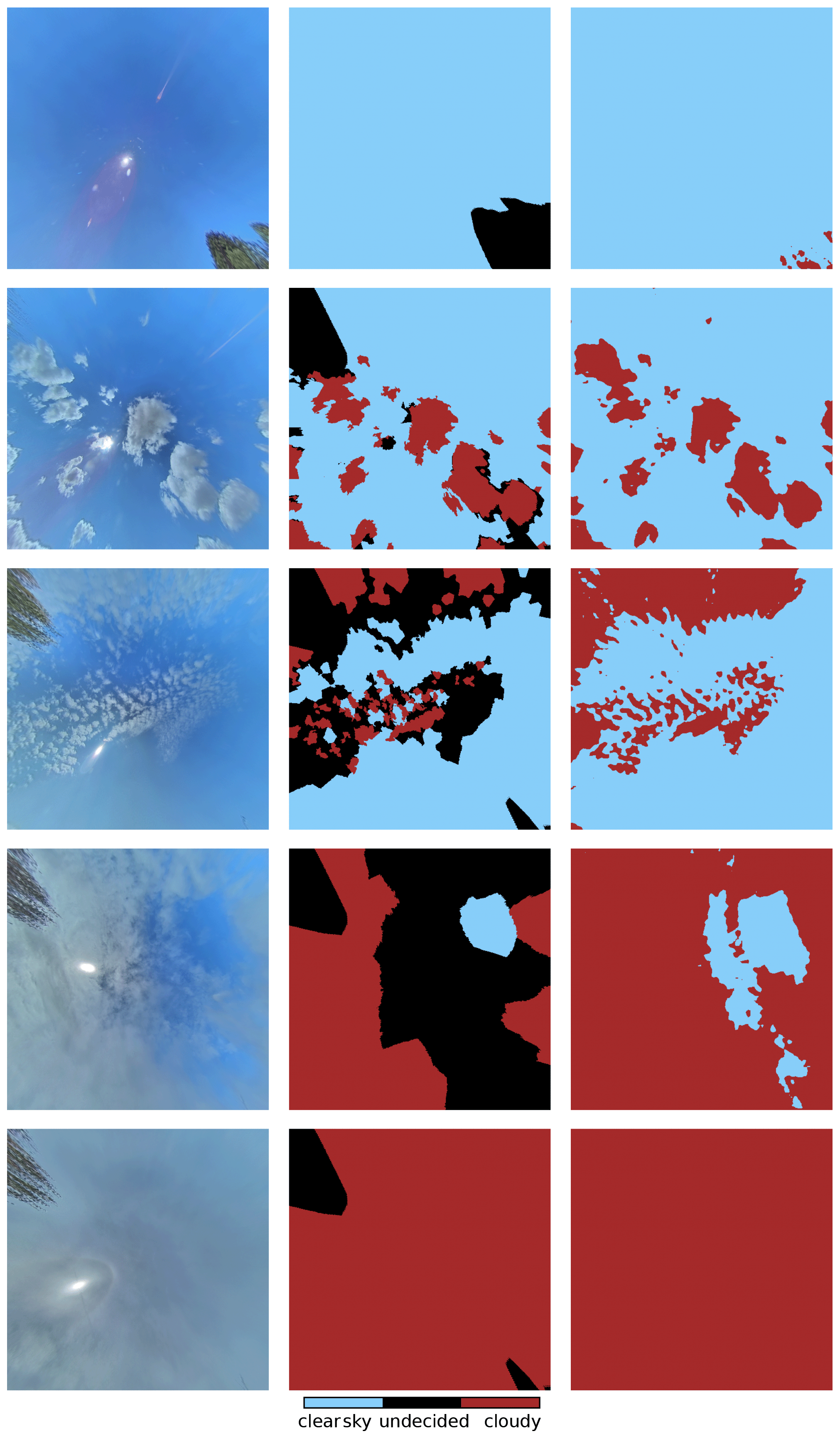
Figure A1 Example images from the validation set (left column) hand-labeled segmentation (middle column), and cloud mask predicted by the trained CNN (right column).

We chose the DeeplabV3+ (Chen et al., 2018) CNN architecture which is designed using an encoder–decoder structure, as is the U-Net architecture (Ronneberger et al., 2015) used by Fabel et al. (2022). For the encoder, we use a ResNet34 (He et al., 2015) pre-trained on the ImageNet dataset (Russakovsky et al., 2014). Three output channels were chosen associated with the three classes. Training was done using the Adam optimizer (Kingma and Ba, 2014) with a custom sparse soft cross-entropy loss (ssce). This ssce actively ignores pixels that are labeled as undecided in the ground truth and only focuses on cloudy and clear pixels. This is done using the following:

$$\begin{array}{}\text{(A1)}& y_{\mathrm{mask},i,j}=\mathrm{1}-y_{\mathrm{gt},i,j,\mathrm{undecided}},\end{array}$$

$$\begin{array}{}\text{(A2)}& \mathrm{LogSoftmax}\left(y_{i,j,c}\right)=\log \left({\displaystyle \frac{\exp \left(y_{i,j,c}\right)}{{\sum }_d\exp \left(y_{i,j,d}\right)}}\right),\end{array}$$

$$\begin{array}{}\text{(A3)}& \begin{array}{rl}{\mathrm{ssce}}_{i,j}& =\sum _{c\in \mathit{\{}\mathrm{cloudy},\mathrm{clear}\mathit{\}}}\mathrm{LogSoftmax}\left(y_{\mathrm{pr},i,j,c}\right)\\ & \cdot y_{\mathrm{gt},i,j,c}\cdot y_{\mathrm{mask},i,j},\end{array}\end{array}$$

where $y_{\mathrm{pr},i,j,c}$ is the predicted value for the ith pixel of the jth training image and the class c. Correspondingly, $y_{\mathrm{gt},i,j,c}\in \left\{\mathrm{0},\mathrm{1}\right\}$ is the ground truth value. While ssce is necessary for optimization, this loss is meant to give mainly intermediate scores of performance of the segmentation CNN. Therefore, a metric called mean intersection over union (mIoU) is also used in a sparse version as follows:

$$\begin{array}{}\text{(A4)}& \mathrm{I}=\sum _{i,j}\sum _{c\in \mathit{\{}\mathrm{cloudy},\mathrm{clear}\mathit{\}}}{y}_{\mathrm{gt},i,jc}\cdot y_{\mathrm{pr},i,j,c}\cdot y_{\mathrm{mask},i,j},\end{array}$$

$$\begin{array}{}\text{(A5)}& \mathrm{U}=\sum _{i,j}\sum _{c\in \mathit{\{}\mathrm{cloudy},\mathrm{clear}\mathit{\}}}\left(y_{\mathrm{gt},i,j,c}+y_{\mathrm{pr},i,j,c}\right)\cdot y_{\mathrm{mask},i,j}-\mathrm{I},\end{array}$$

$$\begin{array}{}\text{(A6)}& \mathrm{mIoU}={\displaystyle \frac{\mathrm{I}}{\mathrm{U}+\mathit{ϵ}}},\end{array}$$

with $\mathit{ϵ}={\mathrm{10}}^{-\mathrm{7}}$ for numerical stability. This metric is designed to represent a ratio between correctly classified pixels in comparison to overall classified pixels, again adapted by us to ignore undecided ground truth pixels. It was computed after every epoch on the entire validation dataset. We used a batch size of 26 images and a learning rate of $\mathrm{7}\times {\mathrm{10}}^{-\mathrm{5}}$. After 48 epochs of training, mIoU=0.968 was reached for the CNN as used within this study. For the prediction of cloud masks, the label of a pixel is derived from the output channel with the maximum value. This is mapped to scalar values as 0 for clear, 1 for cloudy, and 0.5 for undecided to obtain the final CNN cloud masks.