A unified synergistic retrieval of clouds, aerosols, and precipitation from EarthCARE: the ACM-CAP product

ACM-CAP provides a synergistic best-estimate retrieval of all clouds, aerosols, and precipitation detected by the atmospheric lidar (ATLID), cloud-profiling radar (CPR), and multi-spectral imager (MSI) aboard EarthCARE (Earth Cloud Aerosol and Radiation Explorer). While synergistic retrievals are now mature in many contexts, ACM-CAP is unique in that it provides a unified retrieval of all hydrometeors and aerosols. The Cloud, Aerosol, and Precipitation from mulTiple Instruments using a VAriational TEchnique (CAPTIVATE) algorithm allows for a robust accounting of observational and retrieval errors and the contributions of passive and integrated measurements and for enforcing physical relationships between components (e.g. the conservation of precipitating mass flux through the melting layer).

We apply ACM-CAP to EarthCARE scenes simulated from numerical weather model forecasts and evaluate the retrievals against “true” quantities from the numerical model. The retrievals are well-constrained by observations from active and passive instruments and overall closely resemble the bulk quantities (e.g. cloud water content, precipitation mass flux, and aerosol extinction) and microphysical properties (e.g. cloud effective radius and median volume diameter) from the model fields. The retrieval performs best where the active instruments have a strong and unambiguous signal, namely in ice clouds and snow, which is observed by both ATLID and CPR, and in light to moderate rain, where the CPR signal is strong. In precipitation, CPR's Doppler capability permits enhanced retrievals of snow particle density and raindrop size. In complex and layered scenes where ATLID is obscured, we have shown that making a simple assumption about the presence and vertical distribution of liquid cloud in rain and mixed-phase clouds allows improved assimilation of MSI solar radiances. In combination with a constraint on the CPR path-integrated attenuation from the ocean surface, this leads to improved retrievals of both liquid cloud and rain in midlatitude stratiform precipitation. In the heaviest precipitation, both active instruments are attenuated and dominated by multiple scattering; in these situations, ACM-CAP provides a seamless retrieval of cloud and precipitation but is subject to a high degree of uncertainty. ACM-CAP's aerosol retrieval is performed in hydrometeor-free parts of the atmosphere and constrained by ATLID and MSI solar radiances. While the aerosol optical depth is well-constrained in the test scenes, there is a high degree of noise in the profiles of extinction. The use of numerical models to simulate test scenes has helped to showcase the capabilities of the ACM-CAP clouds, aerosols, and precipitation product ahead of the launch of EarthCARE.

1 Introduction

The scientific goals of the EarthCARE (Earth Cloud Aerosol and Radiation Explorer) mission are to measure the global distribution of clouds, aerosols, and precipitation, to estimate their quantities and microphysical properties, and to quantify their radiative effects (Wehr et al., 2023). Within the European Space Agency (ESA) EarthCARE production model (Eisinger et al., 2023), the ACM-CAP product provides the best-estimate retrieval of clouds, aerosols, and precipitation from the synergy of the atmospheric lidar (ATLID), cloud-profiling radar (CPR), and multispectral imager (MSI). The retrieval framework underlying ACM-CAP is the Cloud, Aerosol, and Precipitation from mulTiple Instruments using a VAriational TEchnique (CAPTIVATE; Mason et al., 2017, 2018) algorithm, which is configurable for any combination of vertically pointing radars, lidars, and radiometers. ACM-CAP exploits the complementary properties of EarthCARE's Doppler-capable CPR, high-spectral resolution ATLID, and solar and thermal infrared MSI channels to simultaneously retrieve all classes of hydrometeors and aerosols in each profile and takes account of measurement errors and physical assumptions to report the uncertainties associated with all retrieved quantities for interpretation by users and downstream products. As is more fully described in Eisinger et al. (2023), ACM-CAP forms the basis for subsequent EarthCARE products quantifying the cloud–aerosol–precipitation interactions with radiation by means of radiative transfer modelling for estimating broadband fluxes and heating rates (ACM-RT; Cole et al., 2022) and the top-of-atmosphere radiative closure assessment (ACMB-DF; Barker et al., 2023) when compared against EarthCARE's broadband radiometer (BBR).

Owing to the long-term success of the Afternoon Train (A-Train) of active and passive spaceborne remote sensors, algorithms exploiting the synergy of radars, lidars, and radiometers to retrieve the properties of ice clouds and snow, rain, or liquid clouds can now be considered mature. The active sensors in the A-Train facilitated an unprecedented survey of the atmosphere (Stephens et al., 2018), with the 94 GHz cloud-profiling radar aboard CloudSat (Stephens et al., 2002), detecting ice clouds and snow, drizzle, and light rain, and the 532 nm Cloud–Aerosol Lidar and Orthogonal Polarization (CALIOP) aboard Cloud–Aerosol Lidar and Infrared Pathfinder Satellite Observation (CALIPSO; Winker et al., 2003), detecting optically thin ice clouds, liquid clouds, and aerosols. They were complemented by two radiometers aboard Aqua, namely the Moderate Resolution Imaging Spectroradiometer (MODIS; Salomonson et al., 2002), providing solar and infrared radiances from clouds and aerosols across a wide swath, and the Clouds and the Earth's Radiant Energy System (CERES; Wielicki et al., 1998) broadband radiometer, measuring radiative fluxes at the top of the atmosphere. Single-instrument retrievals can be especially subject to uncertainties in complex or layered scenes – a limitation that multiple-instrument synergies help to overcome. For example, MODIS cloud retrievals are subject to biases in the presence of drizzle (e.g. Zhang and Platnick, 2011; Painemal and Zuidema, 2011), in mixed-phase clouds (e.g. Khanal and Wang, 2018), and in layered cloud scenes (e.g. Chang and Li, 2005; Naud et al., 2006). Similarly, CloudSat rain retrievals are subject to uncertainties due to liquid clouds, which contribute to radar attenuation (Leinonen et al., 2016; Matrosov, 2007; Matrosov et al., 2008), and CloudSat ice and snow retrievals are often blind to the presence of supercooled liquid cloud (Battaglia and Delanoë, 2013; Battaglia and Panegrossi, 2020). In synergistic retrievals, complementary measurements can be used to constrain multiple classes of hydrometeors simultaneously; for example, CloudSat and MODIS solar radiances are used to retrieve rain (Lebsock et al., 2011) and cloud water content (Austin et al., 2009; Leinonen et al., 2016). Synergistic retrievals can also be used to constrain additional properties within a class of hydrometeors; in ice clouds and snow, the complementary constraints of the radar reflectivity factor and lidar backscatter provide sufficient information to retrieve two parameters of the particle size distribution. DARDAR-CLOUD (Delanoë and Hogan, 2008, 2010) uses CloudSat, CALIPSO, and MODIS thermal infrared radiances to retrieve the profile of ice cloud and snow, with infrared radiances providing an integrated constraint on ice microphysical properties near the cloud top. Building upon the heritage of A-Train retrievals, and specifically on the optimal estimation approach used by DARDAR-CLOUD, ACM-CAP will take advantage of EarthCARE's on board synergy to assimilate all available ATLID, CPR, and MSI measurements and to retrieve all combinations of clouds, aerosols, and precipitation simultaneously.

While the A-Train has yielded many single-instrument and synergistic retrievals, each product has been concerned with a subset of the full range of hydrometeors or aerosols in the atmosphere; therefore, several data products must be combined in order to reconstruct the full distribution of clouds, aerosols, and precipitation in the atmosphere and estimate their combined effects on the global radiation budget. The prominent effort to collate the A-Train retrievals and radiative transfer products based on composites of retrievals (Henderson et al., 2013) in the context of radiative flux measurements from CERES is the CALIPSO–CloudSat–CERES–MODIS product (CCCM; Kato et al., 2010, 2011). CCCM has been widely used to link profiles of clouds and aerosols to atmospheric heating rates and cloud radiative effects (e.g. Hill et al., 2018; Ham et al., 2017); however, a challenge when combining retrievals is that the different products are neither necessarily based on consistent physical assumptions, nor do they account for consistent contributions from each measurement. As a consequence, the uncertainties in the retrieved quantities, and hence the derived radiative fields, are difficult to quantify (Kato et al., 2011). The ACM-CAP product is novel in that all classes of hydrometeors and aerosols are retrieved simultaneously. This maximizes the exploitation of EarthCARE instrument synergy and allows the application of physical relationships between different parts of the retrieval. For example, retrieving snow and rain simultaneously means that a physical consistency condition can be applied to ensure that the precipitation mass flux is conserved across the melting layer, as has been used in radar precipitation retrievals (Haynes et al., 2009; Mason et al., 2017; Mróz et al., 2021). In complex and layered scenes, some integrated or passive measurements cannot be adequately interpreted by species-specific retrievals. A unified approach ensures that the contributions of such constraints – for example, radar attenuation due to rain and liquid cloud or solar radiance measurements with contributions from multiple cloud or aerosol layers – are applied consistently. This allows for high-quality retrievals in the profiles where species-specific algorithms are most likely to report biased retrievals, large uncertainties, or to skip profiles entirely. Moreover, using a single retrieval framework has the advantage of facilitating a detailed and consistent accounting of all measurement errors, uncertainties related to physical assumptions, and uncertainty estimates for all retrieved quantities. Retrieval uncertainties can be easily interpreted by users of the product, and included in downstream radiative transfer (ACM-RT; Cole et al., 2022) products.

In addition to its A-Train like measurements, EarthCARE's active instruments will have novel capabilities that will enhance the potential for cloud, aerosol, and precipitation retrievals with ACM-CAP. The CAPTIVATE algorithm has already been used to demonstrate how Doppler radars to retrieve information about the structure and density of snowflakes (Mason et al., 2018, 2019) and about the rain drop size distribution (Mason et al., 2017). The high-spectral-resolution lidar (HSRL) capability of ATLID allows for more accurate retrievals of the profile of extinction, while the combined aerosol depolarization ratio and extinction-to-backscatter ratio are used for the advanced aerosol typing (Donovan et al., 2023b; Wandinger et al., 2023) that informs the target classification (AC-TC; Irbah et al., 2023).

In this study, we describe the ACM-CAP processor and evaluate its performance over three synthetic EarthCARE scenes produced from a numerical weather model. Section 2 provides an outline of the ACM-CAP processor within the ESA EarthCARE production model (Eisinger et al., 2023), a detailed description of the retrieval framework, its representation of ice cloud and snow, liquid cloud, rain and aerosols, and its instrument forward models. In Sect. 3, we showcase and evaluate ACM-CAP using case studies in selected cloud, precipitation, and aerosol regimes, and in Sect. 4, we present a statistical evaluation of key retrieved quantities across the three test scenes. Finally, in Sect. 5, we summarize the outlook for ACM-CAP and EarthCARE science.

2 ACM-CAP product

The CAPTIVATE retrieval scheme employs a classical variational (or optimal estimation) approach (Rodgers, 2000) but is unique in that almost all aspects of the retrieval are configurable at runtime, including the observations to assimilate, the representation of the atmospheric constituents to retrieve (ice clouds and snow, liquid clouds, rain, and aerosols), the state variables used to describe each constituent, and the additional constraints to apply. This means that the same algorithm can be applied to ground-based (Mason et al., 2018, 2019), airborne (Mason et al., 2017), and spaceborne platforms. In Sect. 2.1, we provide an overview of how CAPTIVATE is configured for its application as the ACM-CAP processor, and then we describe the representation of atmospheric constituents (Sect. 2.2) and the forward models for the EarthCARE instruments (Sect. 2.3).

2.1 Algorithm overview

Each EarthCARE orbit is divided into eight granules of length ∼ 5000 km; the ACM-CAP processor runs one granule at a time, reading in six Level 1 and Level 2 data products and outputting one ACM-CAP data product for each granule. The ACM-CAP processor and its inputs and outputs are illustrated in Fig. 1.

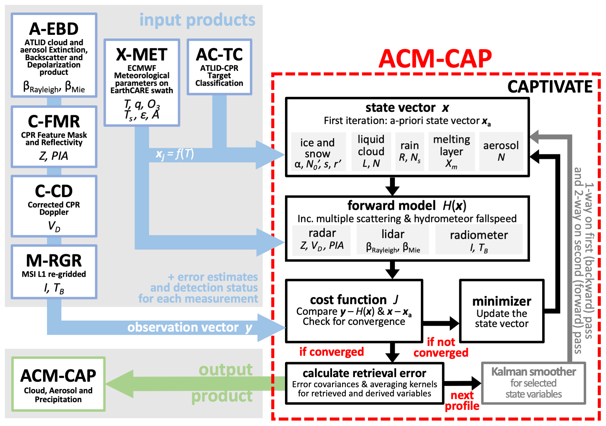
Figure 1 Flowchart showing the ACM-CAP processor and its input and output data products. The ACM-CAP processor uses the CAPTIVATE retrieval framework configured for EarthCARE's ATLID, CPR and MSI instruments.

Each profile in the granule is processed in turn. The synergistic target classification product (AC-TC; Irbah et al., 2023) is used to define which constituents will be retrieved in each grid volume. Each retrieved constituent is described by a number of state variables, the selection of which is described in Sect. 2.2. We write the vector of state variables describing a profile of constituent j as x_j, and if we are retrieving the properties of n different constituents, then the vectors are concatenated to obtain the full state vector x.

The forward model H(x) is used to simulate the observations made by each instrument based on the state. In Sect. 2.3, we describe how the state variables are used to forward model the measurements of active and passive instruments at a range of wavelengths. The forward model requires additional information about the atmosphere provided by the auxiliary X-MET product (see Sect. 5 of Eisinger et al., 2023), which contains atmospheric profiles of temperature, humidity, and trace gas concentrations, as well as surface temperature and albedo, extracted from the operational European Centre for Medium-Range Weather Forecasts (ECMWF) forecast in the proximity of each EarthCARE granule. These data are used to estimate clear-air absorption and scattering properties needed in the various forward models.

Each instrument makes a certain number of usable measurements in a profile, and we write the vector of usable measurements by instrument i as y_i. If we are assimilating the measurements by m different instruments, then the vectors are concatenated to obtain the full observation vector y. These measurements are obtained from the following four input data files:

• A-EBD, which contains the post-processed ATLID backscatter measurements (Donovan et al., 2023a).

• C-FMR, which contains the CPR radar reflectivity and path-integrated attenuation (PIA) measurements (Kollias et al., 2023).

• C-CD, which contains the Doppler velocity measurements (Kollias et al., 2023).

• M-RGR, which contains the regridded MSI reflectances and radiances.

CPR and MSI products are provided on their own instrument grids, while A-EBD is on the joint standard grid (JSG), which is initially defined by the auxiliary X-JSG data product (Eisinger et al., 2023) and then inherited by all ATLID and downstream synergistic Level 2 data products. The JSG provides the common reference grid at 1 km horizontal (along-track) and 100 m vertical resolution onto which all active measurements are mapped. Within the ACM-CAP processor, the CPR and MSI measurements are first interpolated onto the common grid before the retrieval is carried out. To inform the interpretation and assimilation of each measurement, additional variables describing the measurement uncertainties, and quality and detection statuses, are also read from each data product.

The optimal estimate is the state vector that minimizes the cost function

$$\begin{array}{}\text{(1)}& J={\displaystyle \frac{\mathrm{1}}{\mathrm{2}}}\mathit{\delta }{\mathit{y}}^{\mathrm{T}}{\mathbf{R}}^{-\mathrm{1}}\mathit{\delta }\mathit{y}+{\displaystyle \frac{\mathrm{1}}{\mathrm{2}}}\mathit{\delta }{\mathit{x}}^{\mathrm{T}}{\mathbf{B}}^{-\mathrm{1}}\mathit{\delta }\mathit{x}+J_{\mathrm{c}}\left(\mathit{x}\right),\end{array}$$

where, in the first term on the right-hand side, $\mathit{\delta }\mathit{y}=\mathit{y}-H\left(\mathit{x}\right)$, H(x) is the forward model, while $\mathbf{R}=\mathbf{O}+\mathbf{M}$ is the error covariance matrix of δy and consists of the sum of the error covariance matrices of the observations O and the forward model M. In the second term on the right-hand side, $\mathit{\delta }\mathit{x}=\mathit{x}-{\mathit{x}}_{\mathrm{a}}$, where x_a is the prior estimate of the state, and B is the error covariance matrix of these priors. The final term, J_c(x), expresses other physical constraints on the relationship between state variables.

Two methods have been implemented for iteratively modifying the state to minimize the cost function. The first is the L-BFGS method (Liu and Nocedal, 1989), which requires the gradient of the cost function with respect to the state, $\partial J/\partial \mathit{x}$ (a vector), to be computed. This is the approach used by most variational data assimilation systems for which the state vector is very large. The second is the Levenberg–Marquardt method (Marquardt, 1963), which requires both $\partial J/\partial \mathit{x}$ and the second derivative of the cost function with respect to the state ${\partial }^{\mathrm{2}}J/\partial {\mathit{x}}^{\mathrm{2}}$ (a matrix known as the Hessian) to be computed. This curvature information leads to fewer iterations being required, but each iteration is more computationally costly, since the Hessian requires the full Jacobian matrix $\partial \mathit{y}/\partial \mathit{x}$ to be computed. In practice, both the Hessian and Jacobian matrices are computed very efficiently by coding CAPTIVATE in C$++$, making use of the combined array, automatic differentiation, and optimization library Adept (Hogan, 2014, 2017). Both the Levenberg–Marquardt and L-BFGS implementations in Adept support bounding values to be applied to any of the state variables. We presently use the L-BFGS method, having found that it leads to the shortest computational runtime.

The method described so far allows all state variables to be modified in an attempt to minimize J. While we include in CAPTIVATE all the variables needed to describe each constituent, there are not always sufficient measurements to constrain their retrieval; i.e. there may be too many degrees of freedom. In these situations, it is possible to designate a model variable, which is included in the state vector but not modified during the minimization. This reduces the degrees of freedom, while allowing uncertainty in the model variable to be included in the cost function and propagated to the retrieved and derived quantities.

A variational approach provides an elegant framework that takes rigorous account of uncertainties, but the fidelity of any retrieval is dependent on the appropriate choice of state variables and additional constraints and the accuracy of the forward models. In Sect. 2.4, we describe the automatic computation of uncertainties and error covariance matrices for retrieved and derived variables, error correlation scales, and additional metrics derived from the averaging kernel.

We have described the retrieval as being carried out on each profile in turn; however, the retrieval of some state variables may be improved by representing a degree of coherence over larger spatial scales. For these state variables, a Kalman smoother (Rodgers, 2000) can be applied, by which each retrieved profile is constrained on the first pass by the values retrieved in the previous profile and on a second pass by the values retrieved in both directions. Kalman smoothing is especially beneficial for retrieving state variables that are weakly constrained by noisy measurements, such as of aerosols from lidar backscatter.

2.2 Representation of atmospheric constituents

In this section, we describe and justify how each of the atmospheric constituents is represented in ACM-CAP, although we stress that these representations are completely configurable and may be modified as needed. There are several overarching principles that we maintain in selecting state variables:

1. Usually, two variables are used to describe the size distribution, providing the degrees of freedom to allow total number density and mean size to vary. The shapes of the size distributions are configurable but held fixed. The uncertainty associated with a fixed size distribution shape is secondary compared to those of number concentration and mean size (Delanoë et al., 2005) but does become relevant in, for example, triple-frequency radar retrievals (Mason et al., 2019).

2. Typically, we retrieve one extensive variable E (e.g. water content or extinction coefficient) and one variable N that has the properties of a number concentration. This means that only 1D look-up tables are required, since all other extensive variables X can be written as $X/N=f\left(E/N\right)$, while all intensive variables can be written as $I=f\left(E/N\right)$ (see Delanoë et al., 2005, for further discussion).

3. Additionally, convergence is more rapid if the relationship between observations and the main state variables that they are sensitive to is close to linear. Since the relationships between many variables are close to a power law (implemented as look-up tables rather than an actual power law), they can be represented as close to linear if both x and y contain the natural logarithm of meteorological and observational quantities. This is appropriate for properties of the size distribution (e.g. water content, extinction coefficient, backscatter coefficient, and radar reflectivity factor) that can span many orders of magnitude and also ensures that retrieved quantities cannot go negative (Delanoë and Hogan, 2008). This approach is common for cloud radar retrievals (i.e. official CloudSat algorithms; Austin et al., 2009; Leinonen et al., 2016) and also well-suited to applications for radiative transfer, where solar and thermal radiances are more linearly related to the natural logarithm of cloud optical depth.

4. Finally, certain useful a priori and physical constraints can be applied only if a constituent is described by a certain variable. For example, the constraint that the gradient of water content of liquid clouds with height should not exceed the adiabatic rate can only be applied if liquid water content is a state variable.

(Delanoë and Hogan, 2008)(Miles et al., 2000)

Table 1 List of state variables used to describe each of the constituents, with corresponding a priori values and their uncertainties. The only state variable not represented as the natural logarithm of a meteorological quantity is the ice–snow density index. The physical constraints include the vertical representation and horizontal Kalman smoothing.

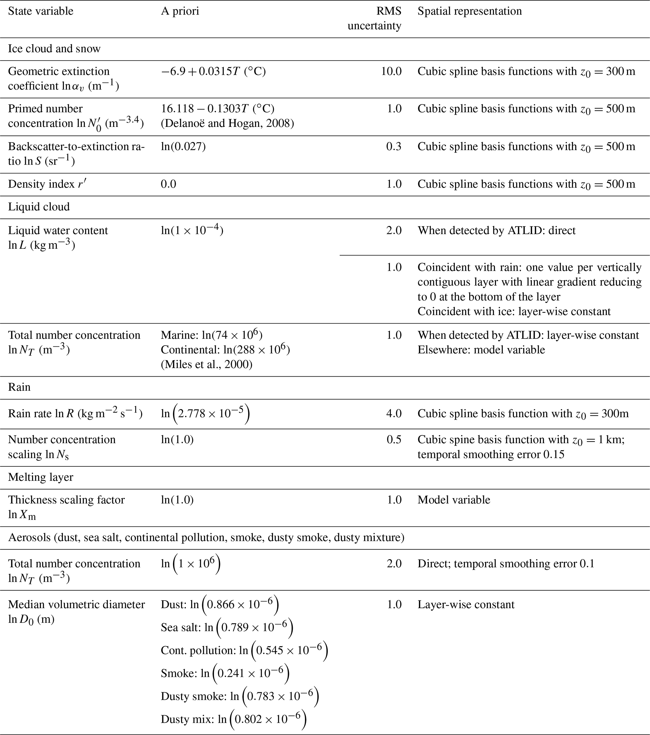
Table 1 lists the state variables retrieved for each atmospheric constituent, along with their a priori values and errors, as presently configured for ACM-CAP. If a state variable is well constrained by an active instrument, then independent values will be retrieved in each volume. However, frequently the observations will lack the information content to retrieve certain state variables at such high vertical resolution, so to ensure that the retrieval is not ill-posed and converges quickly, the profile may optically be described by fewer state variables, such as the coefficients of a set of cubic spline basis functions (Hogan, 2007).

2.2.1 Ice clouds and snow

We follow Delanoë and Hogan (2008) and treat ice clouds and snow as a continuum described by extinction coefficient in the geometric optics approximation, α_v, and a primed number concentration variable, $N_{\mathrm{0}}^{\prime }$, which is defined in terms of the normalized number concentration parameter, $N_{\mathrm{0}}^{\ast }$ (Delanoë et al., 2005). The variable $N_{\mathrm{0}}^{\prime }$ has the advantage that a reasonable a priori estimate of it can be made from temperature alone (Delanoë and Hogan, 2008). This enables a seamless retrieval between regions where both radar and lidar detect the cloud and regions where only one detects it. As ATLID has HSRL capability, its independent information on backscatter and extinction allows vertical variations in the lidar backscatter-to-extinction ratio (S) to be retrieved. This quantity is represented by a cubic spline due to noise in the lidar measurements preventing it from being retrieved reliably at every volume.

Doppler velocity can provide information on the riming of snowflakes, since rimed particles are denser and therefore fall faster than unrimed particles of a similar size. The retrieval of a density factor r to resolve variations in snow particle density due to riming in mixed-phase cloud layers was described in Mason et al. (2018). This single parameter is used to vary the prefactors and exponents of the mass–size and area–size relations of ice particles, in addition to assumptions about the microphysical structure informing microwave scattering approximations. Snow with a density factor of r=0 corresponds to unrimed aggregates with the mass–size relation given by Brown and Francis (1995) and the area–size relation of Francis et al. (1998), while precipitating ice with a density factor of r=1 would correspond to spheres of solid ice. Intermediate values of r represent a continuum of snow particles from partially rimed aggregates to lump graupel. While there are limited observational and theoretical constraints on how to best represent rimed snowflakes and the transition to graupel, CAPTIVATE retrievals of rimed snow from Hyytiälä, Finland, assimilating dual-frequency Doppler radar measurements compared favourably in terms of snow rate and bulk density with in situ snow measurements at the surface (Mason et al., 2018).

In order that the parameter representing riming can be included in the minimization without the possibility of reaching non-physical values, the retrieved state variable is a transformed density factor $r^{\prime }=f\left(r\right)$, which also represents unrimed aggregates at $r^{\prime }=\mathrm{0}$ but is physically meaningful at all values (Sect. 2.2.3 of Mason et al., 2018). This capability has been developed and evaluated using ground-based and dual-frequency Doppler radars. While Mason et al. (2018) demonstrated some skill in using 94 GHz Doppler radars to retrieve rimed snow in stratiform cloud scenes, the capacity to perform this kind of retrieval from EarthCARE is sensitive to the quality of the Doppler velocity measurements. Corrections for radar mispointing and non-uniform beam-filling errors, along-track integration, and more sophisticated local smoothing techniques have been implemented to reduce Doppler velocity measurement noise and decompose an estimate of sedimentation velocity from vertical air motion (Kollias et al., 2023). The choice of which Doppler velocity variable to use in ACM-CAP – and a better characterization of their associated uncertainties – will be informed by calibration and validation activities after launch. The synthetic test scenes used in this study do not include stratiform rimed snow in which to evaluate the contribution of Doppler velocity measurements to snow retrievals in more detail.

2.2.2 Liquid cloud

Liquid clouds present a significant challenge for spaceborne radar and lidar retrievals; while the radar signal is dominated by drizzle drops, the lidar signal is rapidly attenuated at the top of the layer, making the physical depth of a cloud layer difficult to establish. Irbah et al. (2023) have showed that, for EarthCARE, around 20 % of the volume of liquid cloud in the test scenes is directly detected by the synergy of the active instruments, representing around 10 % of the liquid water content. Even when not directly detected by active instruments, integrated constraints on the liquid water path (LWP) – but not on the vertical distribution of liquid – may be obtained from the radar PIA (Lebsock et al., 2011) and on cloud optical depth from solar radiances (Leinonen et al., 2016).

Liquid water content (L) is used as the main state variable, allowing for assumptions about the vertical distribution of cloud water, even in cloud layers that are not directly observed by the active instruments (i.e. non-precipitating clouds not detected by CPR or whenever ATLID is extinguished aloft). In ACM-CAP, liquid cloud is assumed to be coincident with precipitation in the following two situations:

• in rimed snow and convective cores, where the presence of supercooled liquid is very likely and will have a greater contribution to radar attenuation than ice alone; and

• in rain, where liquid cloud is not directly detected by ATLID, but clouds are very likely to be present and will contribute to radar attenuation.

Irbah et al. (2023) showed that this interpretation of the synergistic target classification resulted in the correct classification of around 60 % of the liquid cloud by volume, representing almost 75 % of liquid water content across the three test scenes. The importance of these assumptions, and the capacity to constrain a retrieval of liquid cloud not directly detected by the active instruments, will be explored using case studies in Sect. 3.

The second variable retrieved is the total droplet number concentration, since a priori estimates are available over land and sea (e.g. Miles et al., 2000). When ATLID detects a liquid cloud layer, this variable is retrieved, assuming a constant value for each contiguous cloud layer; otherwise, the a priori value is used.

2.2.3 Rain and drizzle

This constituent represents both cold rain originating from melting ice and warm rain or drizzle from the collision and coalescence of cloud droplets within liquid clouds. The main variable retrieved is the rain rate, R. Since rain has a high fall speed, we can apply the physical constraint that R does not vary rapidly with height, which is achieved by adding a flatness term to J_c that is proportional to ${\left(\partial \ln R/\partial z\right)}^{\mathrm{2}}$, using the approach of Twomey (1977). The result is that, in moderate rainfall, the retrieval can infer rain rates from the gradient of radar reflectivity factor with height (as proposed by Matrosov, 2007), while also being able to use the radar PIA derived from the surface reference technique when available (L'Ecuyer and Stephens, 2002).

The retrieval of warm and cold rain from airborne Doppler radars using CAPTIVATE was demonstrated by Mason et al. (2017). In that study, the second state variable for rain was the normalized number concentration parameter N_w, as defined by Testud et al. (2001) (see also Illingworth and Blackman, 2002). Informed by the mean Doppler velocity and PIA, retrieved values of N_w in that study varied over several orders of magnitude from near the Marshall and Palmer (1948) value of 8 × 10⁶ m⁻⁴ in cold rain to much higher values in warm rain and drizzle. In order that the a priori raindrop size distribution realistically represents both heavy rain and drizzle, in this study we implement the transition between a high concentration of predominantly small drops in drizzle and light rain and fewer and larger raindrops in heavy rain, as described by Abel and Boutle (2012). This relation constitutes our a priori drop size distribution (DSD) for which the number concentration scaling parameter N_s=1 is retrieved as constrained by the mean Doppler velocity and PIA measurements.

2.2.4 Melting layer

Retrieving an accurate physical description of the melting layer is very challenging because we have no direct measurements of its properties, and current models for the scattering and attenuation behaviour of melting ice particles are very uncertain. Since the radar is the only instrument affected by the melting, and there is no enhanced reflectivity bright band at 94 GHz, we treat the melting layer as a thin layer of radar attenuation that is applied across the infinitesimal layer between the lowest volume in the profile classified as ice and snow and the highest volume classified as rain – provided that the two are adjacent. By default, we follow Matrosov (2008) and assume that the two-way attenuation of the melting layer A is proportional to the rain rate R at the first volume just below the melting layer, such that

$$\begin{array}{}\text{(2)}& A=k{X}_{\mathrm{m}}R,\end{array}$$

where, at 94 GHz, k=2.2 dB km⁻¹ (mm h⁻¹)⁻¹. This estimate has been supported using ground-based radars (Li and Moisseev, 2019). The physical depth and hence the total attenuation across the melting layer also depends on the local temperature profile; variations in the strength of the melting layer attenuation can be represented by a thickness scaling factor X_m. Independent information on melting layer attenuation can sometimes be extracted from the combination of the radar PIA over the ocean and the rain rate inferred from the reflectivity gradient; we therefore include the natural logarithm of X_m as either a retrieved state variable or a model variable that resolves the effect of this uncertainty in the other retrieved variables and their errors.

To ensure physical consistency between retrieved constituents within the profile, a constraint can be included in J_c, such that the rain rate in the volume at the bottom of the melting layer is close to the mass flux of snow entering the melting layer. This mass flux continuity constraint has been used before in radar retrievals (Haynes et al., 2009; Mason et al., 2017); further constraints on the continuity of snow and rain microphysical parameters across the melting layer have been demonstrated in multiple-frequency radar retrievals (Mróz et al., 2021) but could prove beneficial even in this application and could be the subject of future work.

2.2.5 Aerosols

The ACM-CAP treatment of aerosols takes as given the aerosol typing and properties of the HETEAC model (Wandinger et al., 2016, 2023), in which all classifications comprise up to four aerosol species, namely fine (strongly and weakly absorbing) and coarse (dust and salt) particles. Predefined mixtures of the HETEAC species map directly to the ATLID aerosol classification (A-TC; Donovan et al., 2023b) and subsequently to the synergistic target classification (AC-TC; Irbah et al., 2023). Look-up tables of the wavelength-dependent scattering properties of the four HETEAC species are combined based on the aerosol classification, using a fixed particle size distribution, and the primary state variable retrieved is the total number concentration, which acts to scale all extensive variables such as aerosol extinction/optical thickness.

A major difficulty with using observations at 1 km along-track resolution is that at this scale the lidar measurements are very noisy, especially when the signal is weak. The traditional approach is to average along-track before performing the retrieval, but this is not satisfactory if clouds are to be retrieved simultaneously at high spatial resolution. The retrieval of aerosols from a noisy lidar signal was the primary motivation for the implementation of the Kalman smoother; in this scenario, along-track smoothing is achieved by performing a first (backward) pass through the data, during which the retrieval of a profile is constrained by the values retrieved in the previous profile, followed by a second forward pass in which the retrieval of a profile is constrained by the values in both directions.

2.3 Instrument forward models

The forward model H(x) is a function that outputs the predicted observations y^f corresponding to a particular estimate of the state vector x. Figure 2 shows the flow of information from x to y^f. After outlining the precalculated hydrometeor scattering and surface properties, the following sections describe the individual steps of forward modelling the instrument measurements from the state.

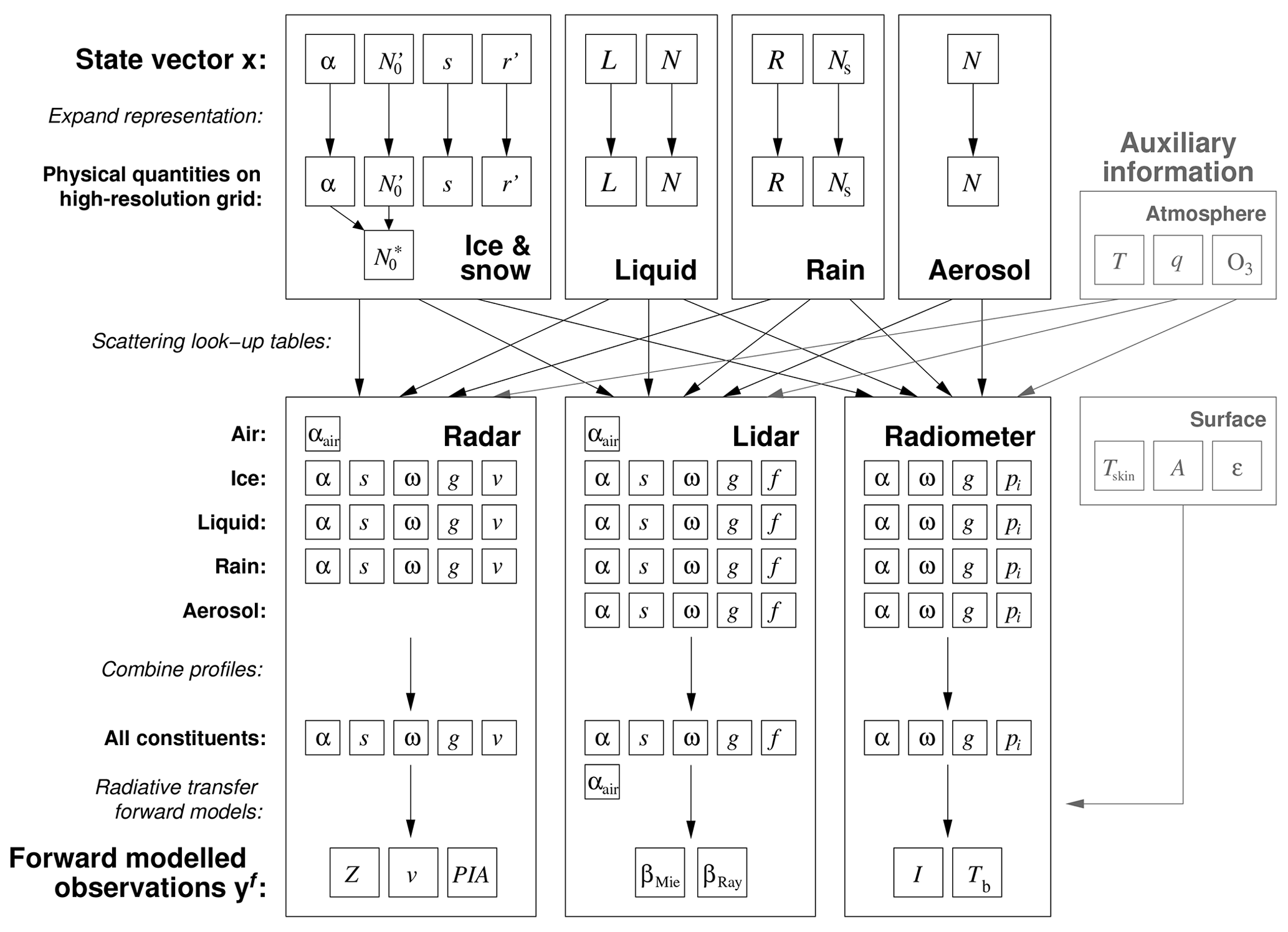
Figure 2 Flowchart depicting the flow of information through the forward model in ACM-CAP, translating the state variables x to the forward modelled observations y^f. Auxiliary information about the state of the atmosphere and Earth's surface is shown in grey. The temperature and composition of the atmosphere are used for forward modelling of the profile of atmospheric scattering at each wavelength, while the surface temperature, albedo, and emissivity are needed to simulate passive measurements. The symbols are defined in Sect. 2.3.

Baran and Francis2004(Hogan et al., 2017)(Mason et al., 2018)Heymsfield and Westbrook (2010)Field et al. (2005)Beard (1976)Beard (1976)Matrosov (2008)(Wandinger et al., 2023)(Wandinger et al., 2023, Table 2)

Table 2 The scattering, fall speed, and size distribution assumptions made for each of the constituents retrieved in ACM-CAP. Certain categories are not applicable (n/a) if an instrument is not able to detect a constituent (e.g. radar and aerosol).

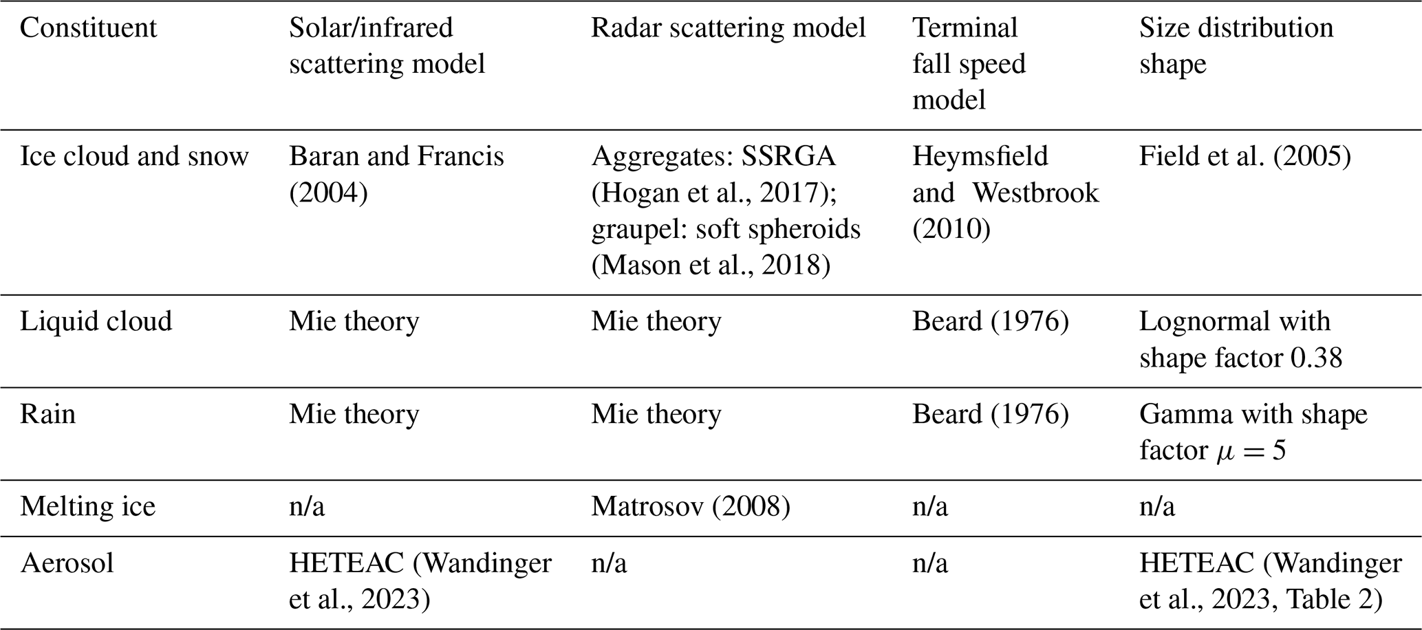
A key part of the forward model is the use of the state variables to calculate the profile of scattering properties at the wavelengths of each instrument being used in the retrieval. Before the retrieval is run, offline calculations are performed to compute the scattering properties of individual hydrometeors, specifically the extinction, scattering, and backscatter cross sections. In the case of solar radiometers, we also compute and store the scattering-phase function. The scattering models used for each constituent are listed in the second and third columns of Table 2. In order to allow the forward modelling of the radar Doppler velocity, we need a model for the terminal fall speeds of hydrometeors detectable to the radar, as given in the fourth column of Table 2.

Since liquid clouds, rain, and spherical aerosol species can reasonably be treated as homogeneous spheres for the wavelengths under consideration, we may use Mie theory. The effect of representing large raindrops with a more realistic spheroidal geometry using the T matrix scattering model had only minor effects on the retrieved rain in Mason et al. (2017) and is neglected here. The complex shapes of ice particles require more detailed careful consideration. For solar and infrared scattering from ice particles, we use the Baran and Francis (2004) database, which takes account of surface roughness effects; however, the backscatter-to-extinction ratio S predicted by such a model is not regarded as being accurate enough for the lidar forward model, so this variable is retrieved (see Sect. 2.2). For radar scattering by unrimed ice particles, we use the Self-Similar Rayleigh–Gans Approximation (SSRGA) model of Hogan et al. (2017), which is appropriate for aggregates and other irregular particles. Following the evidence of Hogan et al. (2012) and others, these particles are assumed to have an aspect ratio of 0.6, to fall with a horizontal alignment, and to follow the mass–size and area–size relations of Brown and Francis (1995) and Francis et al. (1998), respectively. The mass and cross-sectional area of snowflakes are both needed for the fall speed model of Heymsfield and Westbrook (2010). Mason et al. (2018) described how, when Doppler velocity is assimilated, the density factor is used to transition from the unrimed aggregates above to heavily rimed, graupel-like particles, which are represented as homogeneous spheroids for both radar scattering (Hogan et al., 2012) and mass–size and area–size relations. All of these assumptions have uncertainties, which are represented approximately by adding a radar reflectivity forward model error to the appropriate diagonal elements of M (see Eq. 1).

For the forward-modelling of passive solar and infrared radiances in clear-sky and optically thin profiles, we require information about the surface, which is provided in the X-MET product generated from the ECMWF forecast model (Eisinger et al., 2023). For thermal infrared radiances the surface emissivities are taken as constant for wavelengths close to 10 µm, with values of 0.96 over ocean and 0.98 over the land (Fig. 3 of Feldman et al., 2014). The skin temperature is from the same ECMWF forecast that provides the profile of atmospheric temperature and humidity.

In a synergistic retrieval, the absence of a detection from one of the instruments can also convey important information. In volumes where ATLID detects ice clouds but CPR does not make a detection (i.e. classified clear), a pseudo-observation equal to a background noise term is added to both the observation vector of CPR and to the forward-modelled radar reflectivity. This acts as a constraint penalizing the retrieval of ice clouds for which the forward-modelled radar reflectivity would exceed the threshold of detection; it is applied for ice clouds detected only by ATLID, with the effect of reducing the retrieved ice effective radius near the cloud top.

In the following subsections, we describe the steps shown in Fig. 2.

2.3.1 Expanding vertical representation of variables

As indicated in the final column of Table 1, many state variables are not represented by separate values in every volume. Therefore, the first step in the forward model is to expand the representation of each state variable to compute its value in every volume. This process simply involves applying the operation x^full=Wx, where x contains the state variables for a particular quantity, x^full contains the corresponding values in each volume where that constituent is present, and W is a matrix describing the representation. Hogan (2007) describe how W is formulated in the case of cubic splines.

After the state variables are computed in every volume, in the case of ice, we then calculate the normalized number concentration parameter $N_{\mathrm{0}}^{\ast }=N_{\mathrm{0}}^{\prime }{\mathit{\alpha }}_v^{\mathrm{0.6}}$ (Delanoë and Hogan, 2008).

2.3.2 Scattering look-up tables

The next step is to compute the profile of scattering properties for each constituent (ice clouds and snow, liquid clouds, rain, and aerosol) at the wavelength of each instrument. All instruments require the extinction coefficient α, single scattering albedo ω, and asymmetry factor g. The active instruments also require a backscatter-to-extinction ratio S. Furthermore, the Doppler radar requires the reflectivity-weighted terminal fall speed v, and the lidar requires the fraction of the backscatter due to liquid droplets f in order to correctly describe small-angle multiple scattering (Hogan, 2008). Solar radiance modelling requires coefficients describing the full phase function p_i. These quantities are computed from the expanded state variables using look-up tables (see Sect. 2.2). The scattering look-up tables are constructed when the algorithm is initialized.

2.3.3 Combining profiles

The profiles of scattering properties for each constituent, in addition to the profile of scattering due to the atmosphere, are then combined into a single profile for the scattering at each wavelength. The extinction coefficients can be combined as a direct summation, while the other quantities must be combined as weighted sums. The backscatter-to-extinction ratio and single-scattering albedo are combined as weighted by the extinction coefficient, the combined asymmetry factors are weighted by the scattering coefficient (i.e. the extinction coefficient multiplied by the single-scattering albedo), and the droplet fraction and mean Doppler velocity are weighted by the backscatter coefficient (i.e. the extinction coefficient multiplied by the backscatter-to-extinction ratio).

2.3.4 Radiative transfer

The final step in the forward model is to represent the propagation of radiation at all measured wavelengths through the combined profiles of scattering properties due to all hydrometeors, aerosols, and atmospheric gases. To represent ATLID's high-spectral-resolution capability, the Mie attenuated backscatter from hydrometeors and aerosols, and the Rayleigh attenuated backscatter due to air molecules are forward-modelled in separate channels; for all other instruments, the molecular and particulate scattering are combined. For inclusion in the forward model of the retrieval scheme, the radiative transfer model and its adjoint must be calculated accurately and efficiently. All of the radiative transfer methods are therefore written in C$++$ using the Adept automatic differentiation library (Hogan, 2017).

Multiple scattering is accurately treated within the forward model for all active measurements. Millimetre-wave radar is chiefly subject to multiple scattering in deep convective towers, while lidar multiple scattering can occur in all clouds. Wide-angle multiple scattering is modelled for both radar and lidar, using the time-dependent two-stream method (Hogan and Battaglia, 2008). Additional small-angle multiple scattering only affects lidar and is represented using the photon variance–covariance method (Hogan, 2008). The effect of multiple scattering on the radar reflectivity is represented within the radar forward model but not on the mean Doppler velocity; in practice for EarthCARE, Doppler measurements from CPR will not be assimilated wherever multiple scattering has been diagnosed, according to the status variables in the C-FMR and C-CD data products.

In the extreme case of radar attenuation, the surface return is equal to the radar noise, and the measured PIA becomes saturated (Kollias et al., 2023). This results in a maximum PIA measurement, around 60 dB in the heaviest precipitation, being included in the simulated EarthCARE scenes (similar to that observed by CloudSat; the relationship between the PIA and the maximum retrievable precipitation rate for the CloudSat rain retrieval is considered in detail in Haynes et al., 2009). Assimilating the saturated PIA values naively would result in a strong upper limit on the retrieved rain rate; however, not assimilating the saturated PIA values at all would be to discard an important integrated measurement in profiles where both of the active instruments are obscured by multiple scattering and attenuation. We therefore represent the effect of a surface return equal to the radar noise by allowing the forward-modelled PIA to become dominated by a saturation PIA (PIA_sat=60 dB) at high precipitation rates:

$$\begin{array}{}\text{(3)}& \mathrm{PIA}=-\mathrm{10}{\log }_{\mathrm{10}}\left({\mathrm{10}}^{-{\mathrm{PIA}}_{\mathrm{true}}/\mathrm{10}}+{\mathrm{10}}^{-{\mathrm{PIA}}_{\mathrm{sat}}/\mathrm{10}}\right),\end{array}$$

where PIA_true is given in Kollias et al. (2023, Eq. 4). This allows the retrieval to smoothly make use of PIA measurements, even in the heaviest precipitation.

The two-stream source function (TSSF; Toon et al., 1989) approach is used for thermal infrared radiances and has also been applied to model passive microwave radiances, although such measurements are not used in this study. For solar wavelengths, the Forward-Lobe Two-Stream rAdiance Model (FLOTSAM; Escribano et al., 2019) is used, which explicitly models the propagation of radiation that is scattered into the wide forward lobe (of width around 15^∘) that is a characteristic feature of the phase function of most clouds. Radiation that is scattered by larger angles enters the diffuse radiation field and is treated using the two-stream method; thus, FLOTSAM can be thought of as the equivalent of TSSF but for solar wavelengths.

2.4 Calculation of retrieval errors

The state vector that minimizes the cost function is called the solution of the optimal estimation retrieval. Once the cost function is minimized, the errors in the retrieval can be estimated; however, we have often selected as state variables quantities that are not the most physically meaningful, e.g. the primed normalized number concentration parameter $N_{\mathrm{0}}^{\prime }$ for ice and snow. The scattering look-up tables are therefore used to convert the state variables into all of the derived variables that might be of interest to users; as an example, to input the retrieval to a radiative transfer code, we may need to derive a vector d describing the profile of ice water content and effective radius. To compute the retrieval RMS errors in d, we first compute the error covariance matrix of x which is the inverse of the Hessian at the final iteration as follows: ${\mathbf{S}}_{\mathit{x}}={\left({\partial }^{\mathrm{2}}J/\partial {\mathit{x}}^{\mathrm{2}}\right)}^{-\mathrm{1}}$. The error covariance in d is given by S_d=DS_xD^T, where $\mathbf{D}=\mathit{\delta }\mathit{d}/\mathit{\delta }\mathit{x}$ is a Jacobian matrix. The appendix of Delanoë and Hogan (2008) shows that D is very complex to implement manually; however, it is trivial to apply automatic differentiation to d(x) (i.e. the look-up table part of the forward model code) in order to compute D and hence S_d. The square root of the diagonal of S_d then provides the RMSE in d, and error correlations between variables can also be computed.

In addition to the standard deviation error or RMSE for a particular quantity, the error covariance matrix yields the correlation between the errors in the two variables at a particular gate, which is a value between −1 and 1. Second, the width of the diagonal band of the error covariance matrix around an element provides a measure of the vertical error correlation scale (given in metres).

Finally, the averaging kernel given by

$$\begin{array}{}\text{(4)}& \mathbf{A}={\mathbf{S}}_{\mathit{x}}{\mathbf{H}}^{\mathrm{T}}{\mathbf{R}}^{-\mathrm{1}}\mathbf{H}\end{array}$$

provides a measure of the information content of the retrieved state, such that an averaging kernel equal to the identity matrix would describe a retrieval in which all of the retrieved information comes from the observations. The effect of the priors, or of other physical constraints on the retrieval, are reflected by off-diagonal terms. The averaging kernel is used to derive the averaging kernel sum, which reflects the contribution of the observations to the retrieved state and the width of the diagonal, which indicates the smoothing of the retrieval compared to the “true” values (Pounder et al., 2012).

3 Case studies

Three simulated EarthCARE scenes have been produced by applying a state-of-the-art instrument simulator (Donovan et al., 2023b) to a combination of high-resolution Global Environmental Multiscale (GEM) numerical weather forecasts for clouds and precipitation, merged with aerosols extracted from the Copernicus Atmospheric Monitoring Service (CAMS; Qu et al., 2022). The test scenes have proved an invaluable tool for developing, testing, and evaluating EarthCARE retrieval algorithms and the production model (Eisinger et al., 2023). Each scene corresponds to a granule, or roughly 5000 km or one-eighth, of an EarthCARE orbit. The Halifax scene is a Northern Hemisphere midlatitude descending granule that passes over eastern Canada, the western Atlantic Ocean, and the Caribbean. The Baja scene is a Northern Hemisphere midlatitude descending granule that transects the North American continent and ends over the Baja California peninsula. The Hawaii scene is a tropical descending granule over the central Pacific Ocean, beginning near Hawaii.

We have selected cloud, precipitation, and aerosol regimes from within the test scenes as case studies for detailed evaluation. As these scenes have been generated from numerical models, we can access the model variables as “truth” for a more omniscient evaluation than is traditionally possible when using in situ measurements. This will help to demonstrate the performance of ACM-CAP retrievals, in addition to some of the challenges at the limits of the EarthCARE instruments; however, GEM is a numerical model that makes certain microphysical assumptions (e.g. the structure and density of snowflakes and the drop size distribution of rain), which may not always be a good approximation to the real world and which will differ from the prior assumptions and physical representations made in ACM-CAP. The details of some adjustments to the microphysical representation of ice, snow, and supercooled liquid cloud output by the GEM model before input to the instrument simulators are given in Sect. 7 of Qu et al. (2022). As discussed in Qu et al. (2022) and Donovan et al. (2023b), the aerosols in the CAMS model have been mapped to the HETEAC species before simulating the ATLID and MSI measurements. ACM-CAP's representation of aerosols relies on the same HETEAC model but uses predefined mixtures of the HETEAC species to quantify the properties of the six tropospheric aerosol classes which are identified in A-TC (and hence in AC-TC). These and other factors will contribute to the differences between ACM-CAP and the simulated truth from numerical models identified in the evaluation that follows.

3.1 Midlatitude convective and stratiform precipitation

The first case features cold rain in convective and stratiform contexts from the Halifax scene. We show observed and forward-modelled EarthCARE measurements in Fig. 3 and retrieved and model quantities in Fig. 4. The first part of this case is dominated by light-to-moderate cold rain below the stratiform mixed-phase cloud, with tops around 5 km, beneath optically thin ice clouds up to around 12 km. Heavier rain up to 10 mm h⁻¹ is associated with an embedded convective cell around 39.5^∘ N, in which CPR is dominated by multiple scattering and attenuation. The second part of the scene features heavy precipitation up to 20 mm h⁻¹, associated with deep convective clouds reaching around 13 km above sea level; physically and optically thick anvil cloud north of the deep convection overlays a shallow layer of liquid cloud at around 1 km.

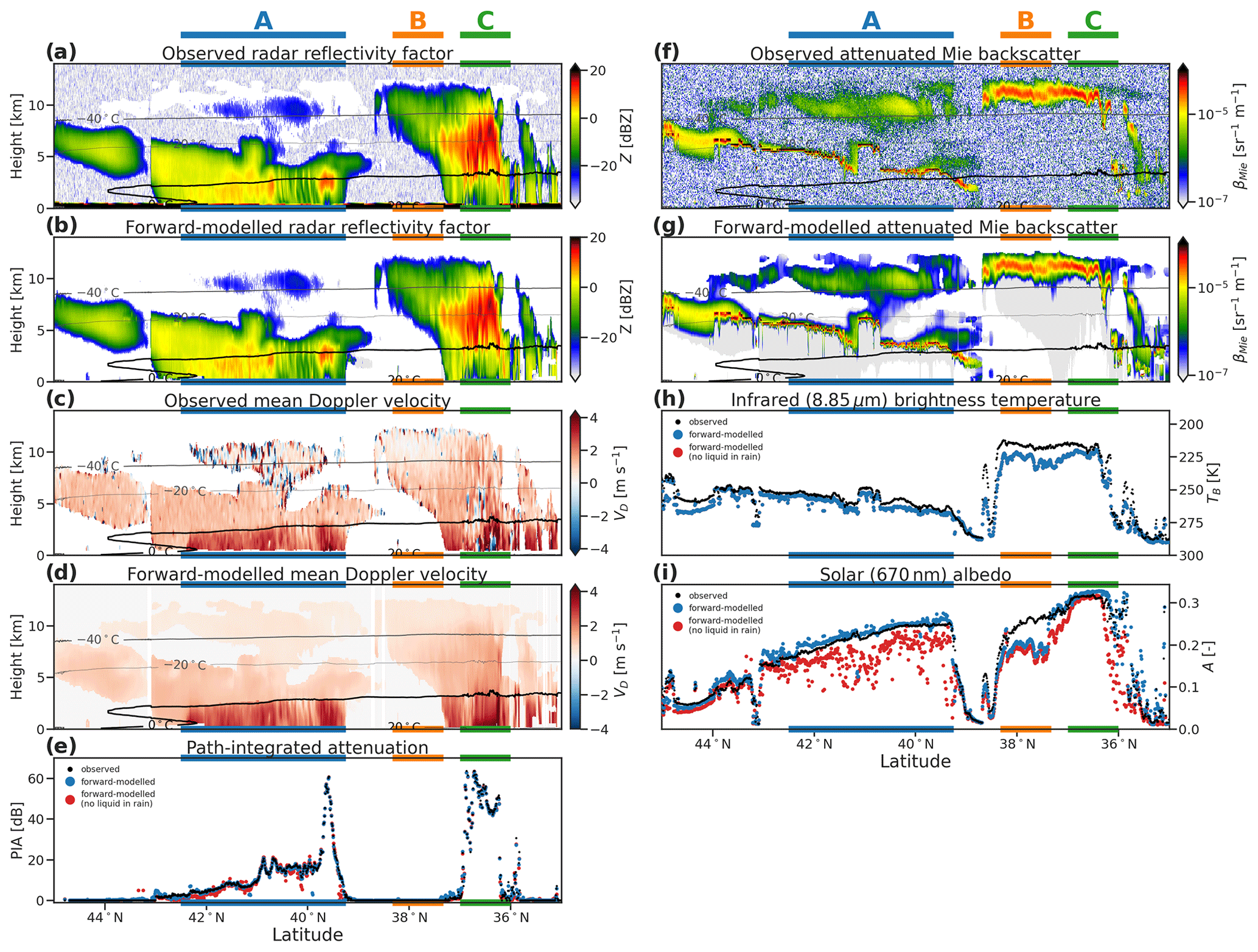
Figure 3 Simulated and forward-modelled CPR reflectivity factor (a, b), mean Doppler velocity (c, d), and PIA (e). ATLID attenuated Mie backscatter (f, g), MSI infrared brightness temperature (h), and solar albedo (i) for the midlatitude stratiform part of the Halifax scene. All profiling variables are overlaid with contours of atmospheric temperature from X-MET. Three areas of interest (A, B, and C) are highlighted.

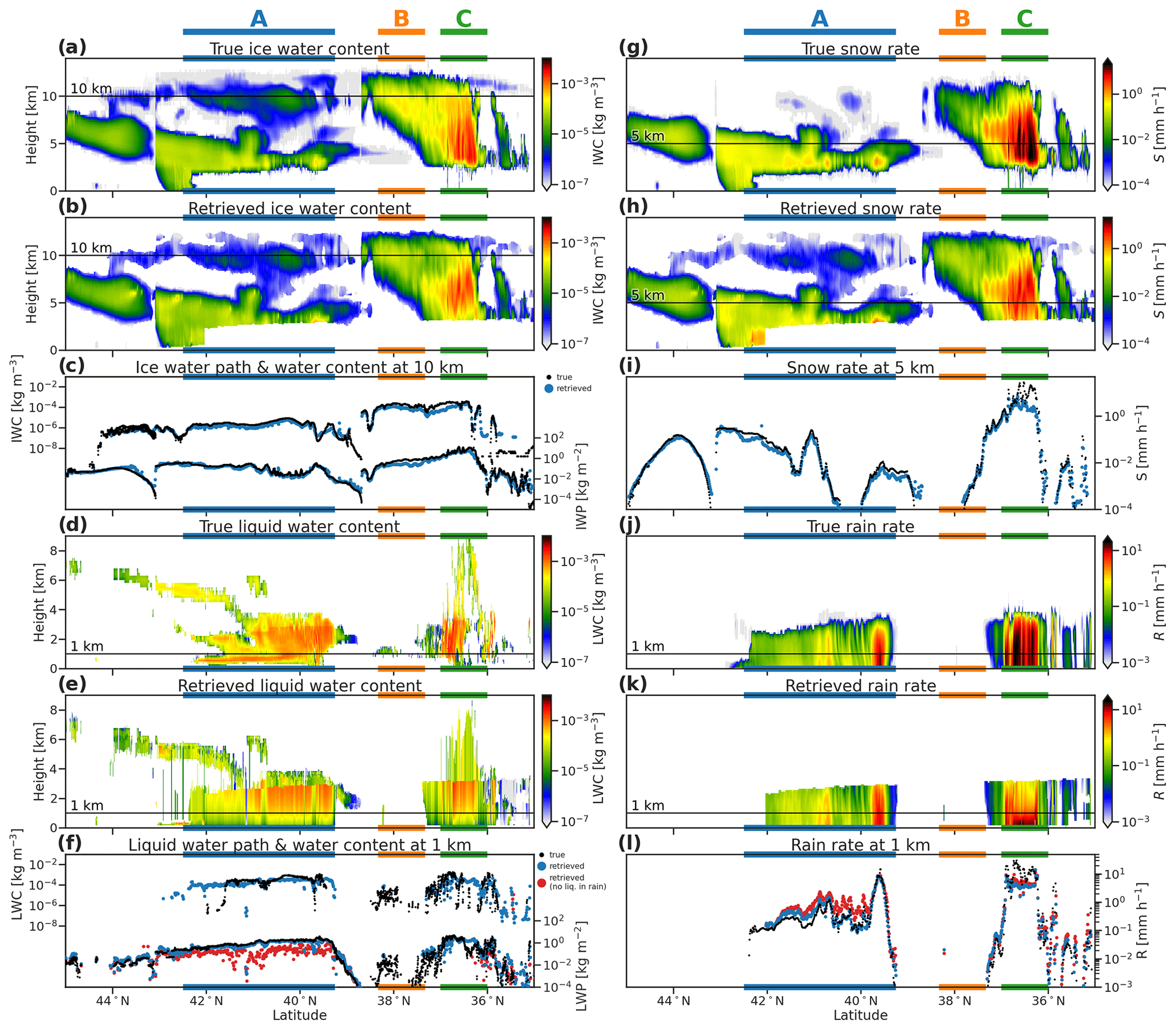
Figure 4 GEM model and ACM-CAP retrievals of IWC (a, b), LWC (d, e), snow rate (g, h), and rain rate (j, k) and comparisons of vertically integrated and selected quantities for ice (c), liquid (f), snow (i), and rain (l) for the midlatitude stratiform part of the Halifax scene. Three areas of interest (A, B, and C) are highlighted.

The CPR and ATLID measurements are accurately forward modelled across this scene at the final iteration of the retrieval (Fig. 3), indicating that the retrieval is well-constrained by the available measurements – but not guaranteeing a unique solution in terms of retrieved quantities. While the overall distribution of ice water content (IWC) is well captured in the retrieval, the retrieved IWC is systematically lower than the GEM model, by around 30 % in the optically thinnest cloud at 10 km above sea level (region A; Fig. 4c). While radar–lidar synergy is available in parts of this cloud, the CPR signal is weak, so the retrieval is primarily constrained by ATLID. IWC is underestimated by as much as 75 % at 10 km above sea level in the deepest ice clouds (region C) and by up to 50 % in the anvil part of the frontal cloud (region B), which is just below the level where lidar signal becomes fully attenuated. Warm biases in infrared brightness temperatures (up to 5 K in region A and up to 10 K regions B and C; note the inverted vertical axis in Fig. 3h) in these regions and elsewhere (e.g. 44 to 45^∘ N, where the snow rate is also underestimated at 5 km; see Fig. 4h) may be related to low IWC reducing the effective radiative level of the clouds and increasing their infrared brightness temperature. These issues may be exacerbated by biases in atmospheric temperature used within the retrieval (X-MET data product, as derived from ECMWF analysis), which can be 1 to 3 K warmer than that of the GEM model, especially in high clouds.

The retrieved snow rates at 5 km above sea level show a better match to the GEM model (Fig. 4i) but include underestimates near the tops of stratiform cloud, such as at the poleward edge of region A. In region C, deficits in retrieved IWC and snow rate are evident where CPR is extinguished; this illustrates the challenge of performing retrievals at the limits of the active sensors and will be explored further in the tropical convection case (Sect. 3.2). While the retrieved snow is not sufficient to attenuate the radar, the retrieved rain rate in region C (Fig. 4j–l) is close to that in the GEM model, at least representing heavy enough rain to saturate the forward-modelled PIA around 60 dB (Fig. 3e).

The forward-modelled ATLID Mie backscatter also broadly reproduces the measurements (Fig. 3g, f) in both optically thin (region A) and optically thick ice clouds (regions B and C), despite the underestimate of IWC. The rapid extinction of ATLID in the mixed-phase cloud-top layer of regime A is somewhat weaker than observed, corresponding to an underestimate in liquid water content (LWC) in parts of these features (Fig. 4d, e).

The bulk of the retrieved liquid cloud, however, is coincident with rain in regions A and C (as described in Sect. 2.2.2), and its retrieval is not constrained by active measurements. Throughout this case, both the LWC at 1 km above sea level and the liquid water path (LWP; Fig. 4f) are remarkably close to the GEM model truth, even in convective precipitation (region C), where the spatial distribution of liquid water in the model is complex (Fig. 4d). As noted above, the deficit of CPR attenuation above the melting layer in region C is related to the deficit of IWC and snow rate. A remedy to this may be a more aggressive assumption to place supercooled liquid throughout convective towers (up to and above 8 km above sea level in the GEM model); however, further tuning of these assumptions should be supported by in-flight data and validation studies rather than a numerical model. To illustrate the effect of retrieving liquid cloud in rain, an ACM-CAP retrieval in which liquid cloud is only retrieved where ATLID detects it is shown in red in Fig. 4f and l. The retrieved LWP throughout region A is underestimated by around an order of magnitude, and the forward-modelled MSI shortwave channel (Fig. 3i) exhibits a 20 % deficit in solar albedo. As both liquid cloud and rain contribute to the attenuation of CPR, which is strongly constrained within the retrieval by PIA, this deficit of liquid cloud is also compensated by an overestimation of rain rate (Fig. 4l). In this stratiform cold-rain regime, solar radiances and radar PIA contribute to an accurate retrieval of LWP and rain rate.

3.2 Deep tropical convection

The equatorial part of the Hawaii scene is dominated by deep tropical cloud, with tops around 18 km and a convective core with extreme precipitation beginning well above the melting level. This case provides an important check on the capacity for synergistic retrievals in heavy precipitation (Fig. 5; region A), where both ATLID and CPR are fully attenuated and passive and integrated measurements become saturated.

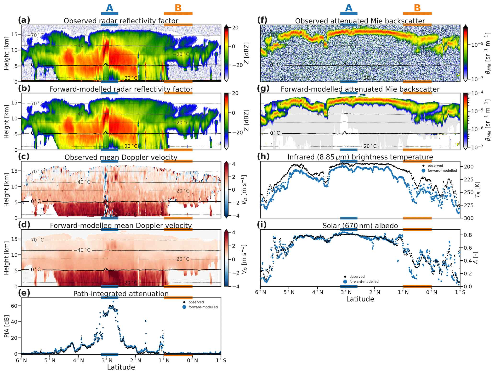
Figure 5 Simulated and forward-modelled CPR reflectivity factor (a, b), mean Doppler velocity (c, d), and PIA (e). ATLID attenuated Mie backscatter (f, g), MSI infrared brightness temperature (h), and solar albedo (i) for the deep convective part of the Hawaii scene. All profiling variables are overlaid with contours of atmospheric temperature from X-MET.

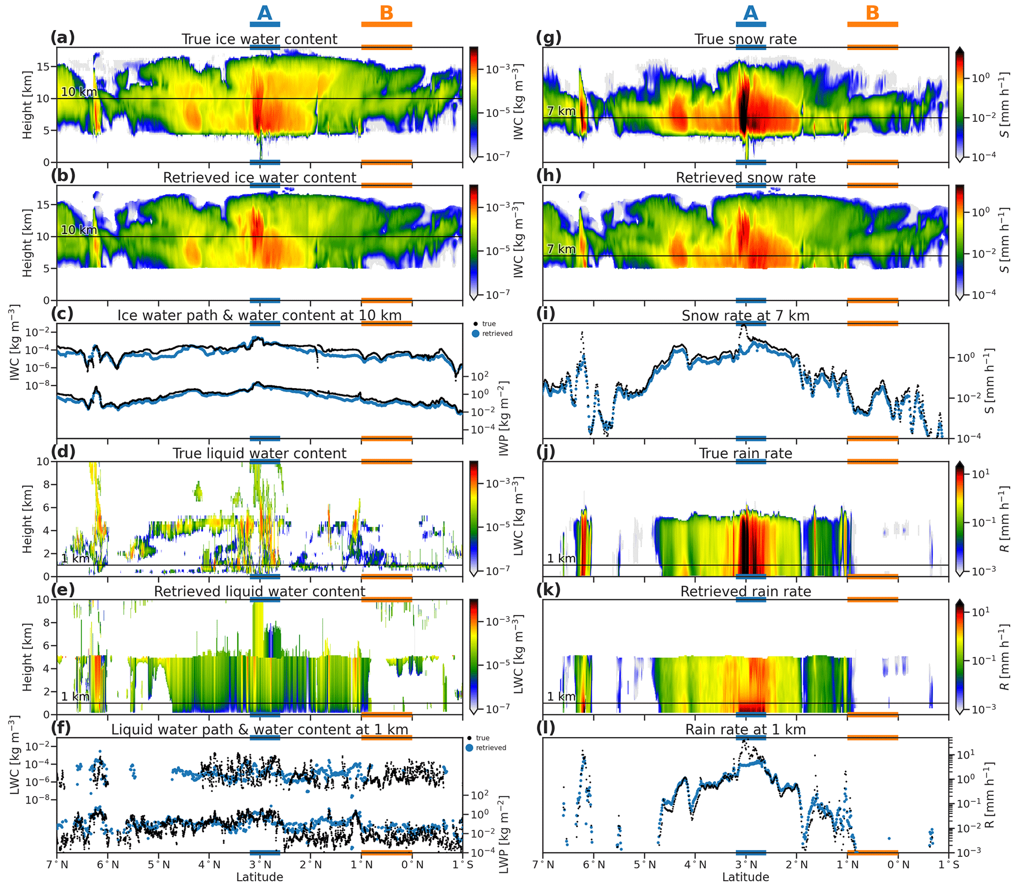
Figure 6 GEM model and ACM-CAP retrievals of IWC (a, b), LWC (d, e), snow rate (g, h), and rain rate (j, k) and comparisons of vertically integrated and selected quantities for ice (c), liquid (f), snow (i), and rain (l) for the deep convective part of the Hawaii scene.

The retrieved IWC at 10 km above sea level (Fig. 6c) and rain rate at 1 km above sea level (Fig. 6l) are remarkably close to the GEM model, except in the convective core (region A). Here the retrieved rain rates are up to 10 mm h⁻¹, whereas the GEM model reaches values of 10 to 30 mm h⁻¹. As noted in the previous case, the greatest challenge is reproducing IWC and snow rate within convective cores, where the radar reflectivity is affected by both attenuation and enhancement due to multiple scattering (Figs. 5a and 6c).

As in the midlatitude stratiform precipitation, the presence and distribution of liquid cloud cannot be constrained by active instruments. The model truth includes a complex field of liquid cloud (Fig. 6d), namely scattered boundary layer clouds around 1 to 2 km and cloud layers close to the melting level and in convective cores reaching from the surface to almost −40 ^∘C. To a greater extent than in the midlatitude case, where the top of a mixed-phase layer was detected by ATLID, the liquid clouds in this scene are almost completely obscured from the active instruments. Using the same approach to indirectly retrieve liquid cloud wherever rain is detected by CPR, the LWC at 1 km above sea level and LWP (Fig. 6f) are close to the GEM model in many parts of this scene (e.g. 5 to 3.5^∘ N) but overestimated in others (2.5^∘ N to 2^∘ S) where the vertical distribution of liquid clouds is more limited. Comparing the forward-modelled solar albedo when liquid cloud is not retrieved in rain (Fig. 6f) shows that this approach can greatly improve the representation of cloud in complex scenes. As in the previous scene, the most extreme mismatches to the MSI solar albedo are beneath non-precipitating ice clouds on either edge of the convective system, where neither liquid clouds nor rain are diagnosed in the target classification but where the GEM model includes shallow layers of low non-precipitating cloud (region B).

3.3 High-latitude mixed-phase clouds

The high-latitude part of the Halifax scene features mixed-phase clouds at night, transitioning from deeper clouds, with tops up to 6 km around 65^∘ N and with supercooled liquid in convective cells, to mixed-phase clouds, with tops around 3 km at temperatures as cold as −30 ^∘C, and, finally, more broken shallow mixed-phase clouds toward 50^∘ N (Fig. 7).

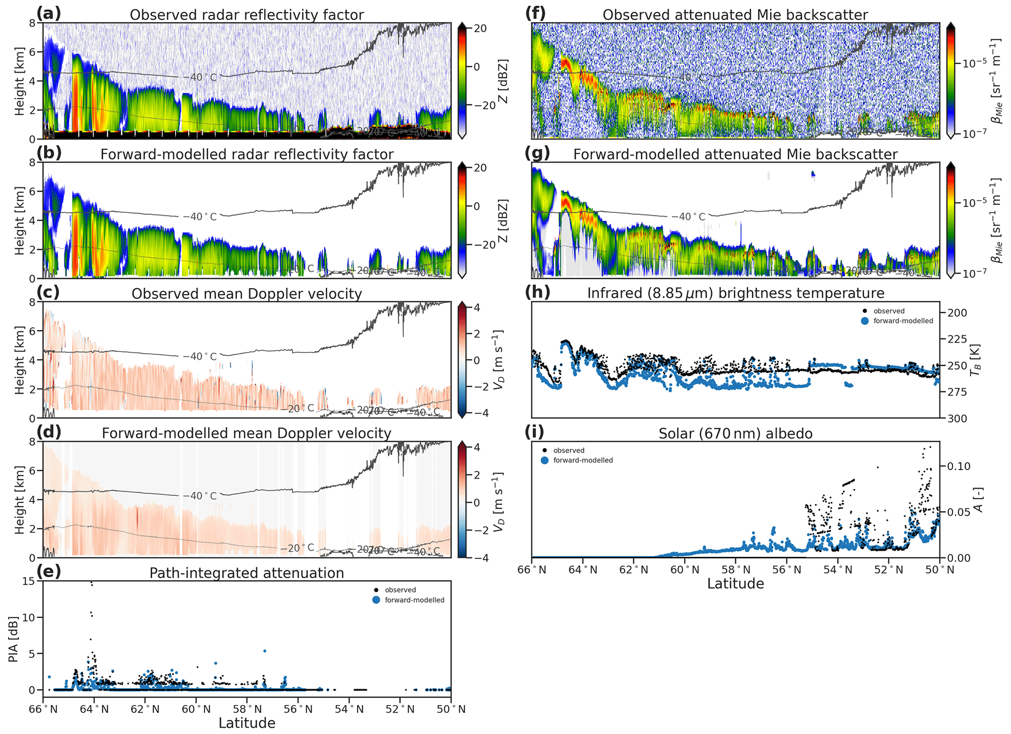
Figure 7 Simulated and forward-modelled CPR reflectivity factor (a, b), mean Doppler velocity (c, d), and PIA (e). ATLID attenuated Mie backscatter (f, g), MSI infrared brightness temperature (h), and solar albedo (i) for the high-latitude mixed-phase part of the Halifax scene. All profiling variables are overlaid with contours of atmospheric temperature from X-MET.​​​​​​​

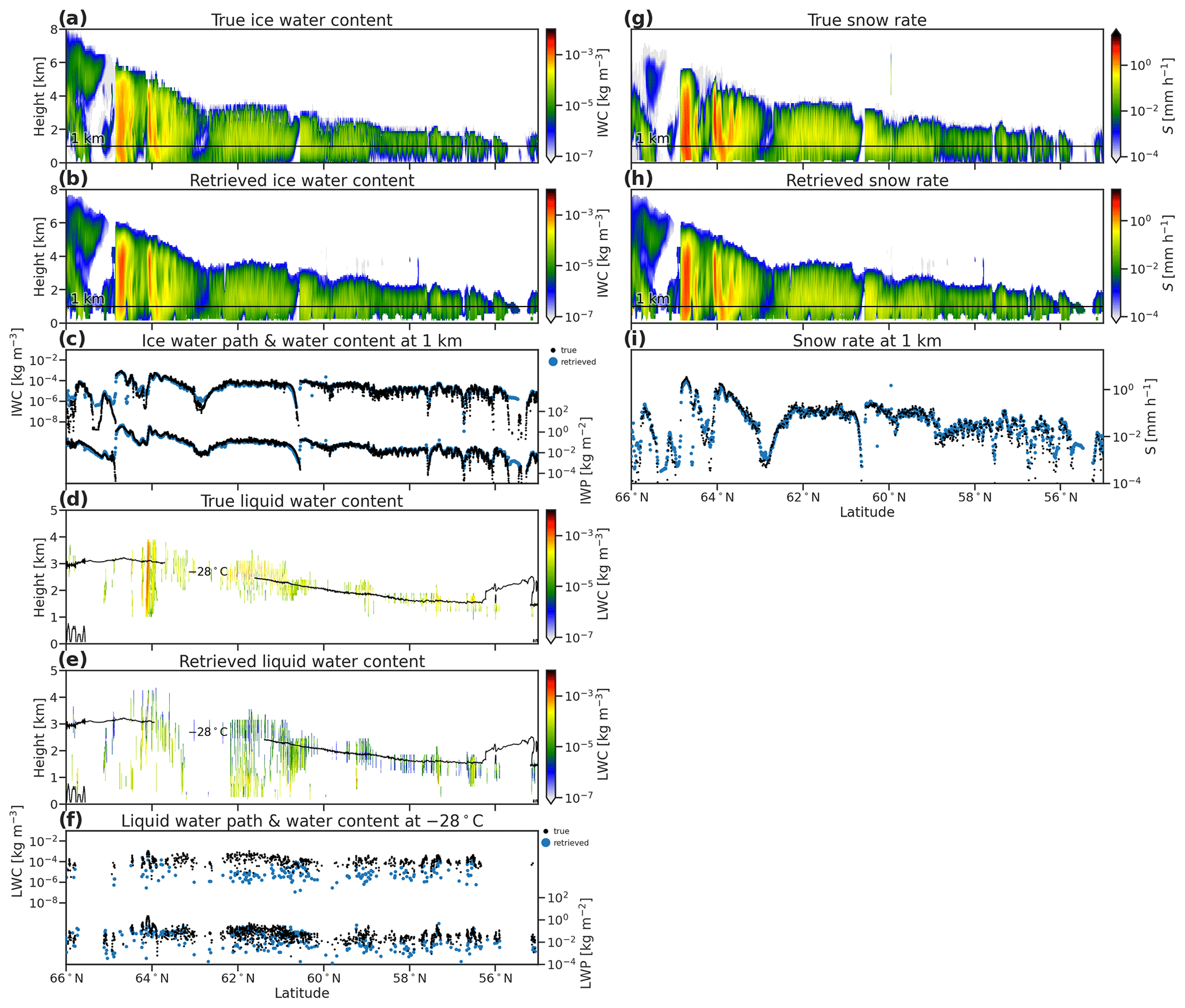
Figure 8 GEM model and ACM-CAP retrievals of IWC (a, b), LWC (d, e), snow rate (g, h), and rain rate (j, k) and comparisons of vertically integrated and selected quantities for ice (c), liquid (f), snow (i), and rain (l) for the high-latitude mixed-phase part of the Halifax scene.

Without solar radiances, the simultaneous retrieval of ice and supercooled liquid is constrained only by the active instruments. The retrieved IWC at 1 km above sea level (Fig. 8c) is close to the model truth throughout the scene, while the retrieved LWC at the −28 ^∘C isotherm (Fig. 8f) is underestimated by 3 orders of magnitude, as is the LWP (Fig. 4f). In day-lit scenes, solar radiances would provide a stronger integrated constraint on liquid water path; the PIA (Fig. 4c) provides little constraint in this part of the scene, where the CPR is only weakly attenuated by supercooled liquid clouds.

3.4 Maritime and continental aerosol layers

The subtropical part of the Halifax scene is dominated by two distinct overlapping layers of aerosols – sea salt from the ocean surface up to 2–4 km, with continental pollution aloft up to 6–8 km – with shallow cumulus clouds embedded in the lowest 2 km. Figure 9 shows the simulated and forward-modelled ATLID and MSI measurements through this scene, and Fig. 10 shows the retrieved aerosol extinction, total aerosol optical thickness, and lidar ratio (LR; i.e. extinction-to-backscatter ratio). We show LR here rather than its reciprocal the backscatter-to-extinction ratio used in the actual retrieval in order to be more easily comparable to other papers in this special issue.

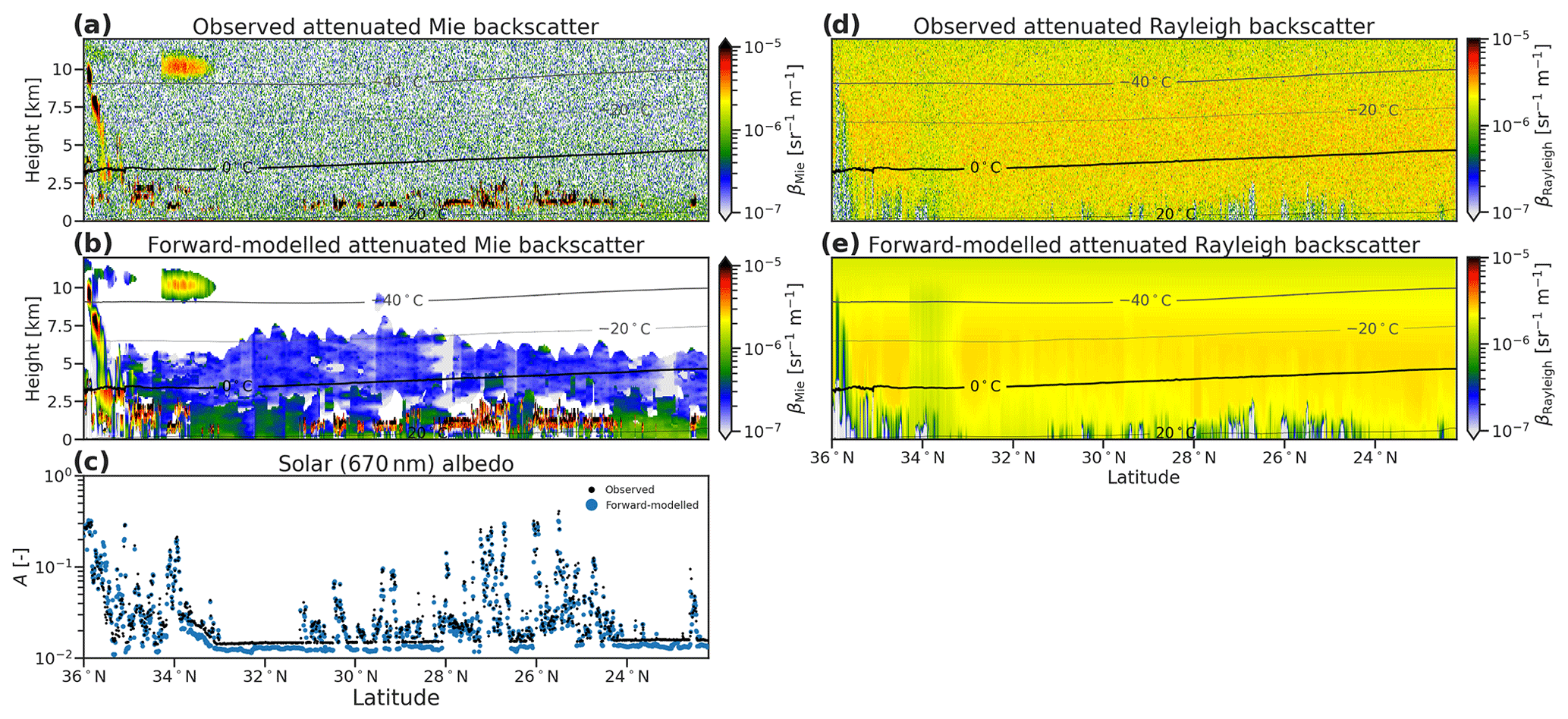
Figure 9 Simulated and forward-modelled ATLID attenuated Mie backscatter (a, b), MSI solar albedo (c), and ATLID attenuated Rayleigh backscatter (d, e) for the subtropical part of the Halifax scene. All profiling variables are overlaid with contours of atmospheric temperature from X-MET.

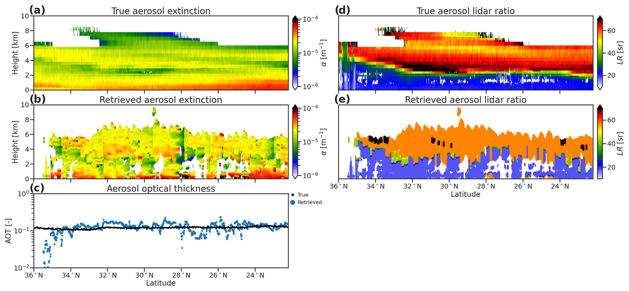
Figure 10 CAMS model and ACM-CAP retrievals of aerosol extinction (a, b) and aerosol optical thickness (c) for the subtropical part of the Halifax scene. Panels (d) and (e) show the corresponding CAMS and ACM-CAP-reported aerosol lidar ratio (i.e. the extinction-to-backscatter ratio); the latter is not retrieved but is a property of each HETEAC aerosol species, as mapped to the CAMS aerosol classes.

The measured ATLID Mie backscatter (Fig. 9a) shows the high degree of measurement noise from which the signal of aerosol backscatter must be detected, which is in contrast to the clear signal from the high ice and liquid boundary layer clouds in the same scene. The forward-modelled Mie backscatter (Fig. 9b) does not contain noise and shows that the signal is often less than 1 × 10⁻⁶ sr⁻¹ m⁻¹.

The retrieved aerosol extinction (Fig. 10b) shows that the retrieval resolves some of the key vertical features within both the sea salt and continental pollution layers; in the sea salt, the strongest extinction is within 1 km of the surface on the equatorward side of the scene, while embedded within the continental pollution layer are 2 km deep structures of stronger extinction. Many horizontal features and discontinuities in the retrieved extinction are not found in the model variables and reflect the challenges of applying a Kalman smoother across large spatial scales when the target classification is interrupted by hydrometeors, which are mostly liquid clouds in this case.

The forward-modelled LR in aerosols (Fig. 10e) shows that the model variables are only coarsely resolved. This illustrates the approach taken within ACM-CAP (and indeed other EarthCARE aerosol algorithms; e.g. Docter et al., 2023) to representing each aerosol class as a mixture of HETEAC species, each with a fixed LR. The result is that some of the structure, especially within the continental pollution layer where LR varies between 50 and 70 sr over around 3 km of the layer, is not resolved. This likely contributes to the overestimated aerosol extinction in the lowest part of the continental pollution layer (around 4 km above the surface between 33–28^∘ N).

4 Statistical evaluation

In addition to case studies, we also evaluate the retrieval statistically in order to diagnose biases and sensitivities. Here we combine all data from the three synthetic EarthCARE granules to evaluate ACM-CAP retrievals of the quantities and properties of ice and snow, liquid clouds, rain, and aerosols against those from the GEM and CAMS models. Strong correlations in retrieved quantities are indicative of the skill of the retrieval. We also statistically compare the forward-modelled and observed measurements from ATLID, CPR, and MSI; strong correlations between these quantities are expected when the retrieval is assimilating EarthCARE measurements as intended.

4.1 Ice and snow

To evaluate the retrieved ice clouds and snow against the GEM model, and the forward-modelled EarthCARE measurements against those simulated from the GEM model, we show probability density functions (PDFs; top panels) and joint histograms (lower panels) of snow rate, IWC, effective radius (Figs. 11), and of measurement variables (Fig. 12). The PDF of all true data (black PDFs) is compared against those in volumes correctly classified by radar–lidar synergy (grey shading; these two will be identical for the measured variables, except due to measurement noise); the difference between these PDFs illustrates the portion of ice clouds that are not recoverable from EarthCARE's instruments. The other PDFs show equivalent quantities retrieved or forward modelled by ACM-CAP everywhere (red lines) and specifically in volumes which do not contain ice or snow in the model (red shading). The joint histograms show the degree to which the retrieved and forward-modelled quantities represent the true values, including correlation coefficients (r) and RMSEs.

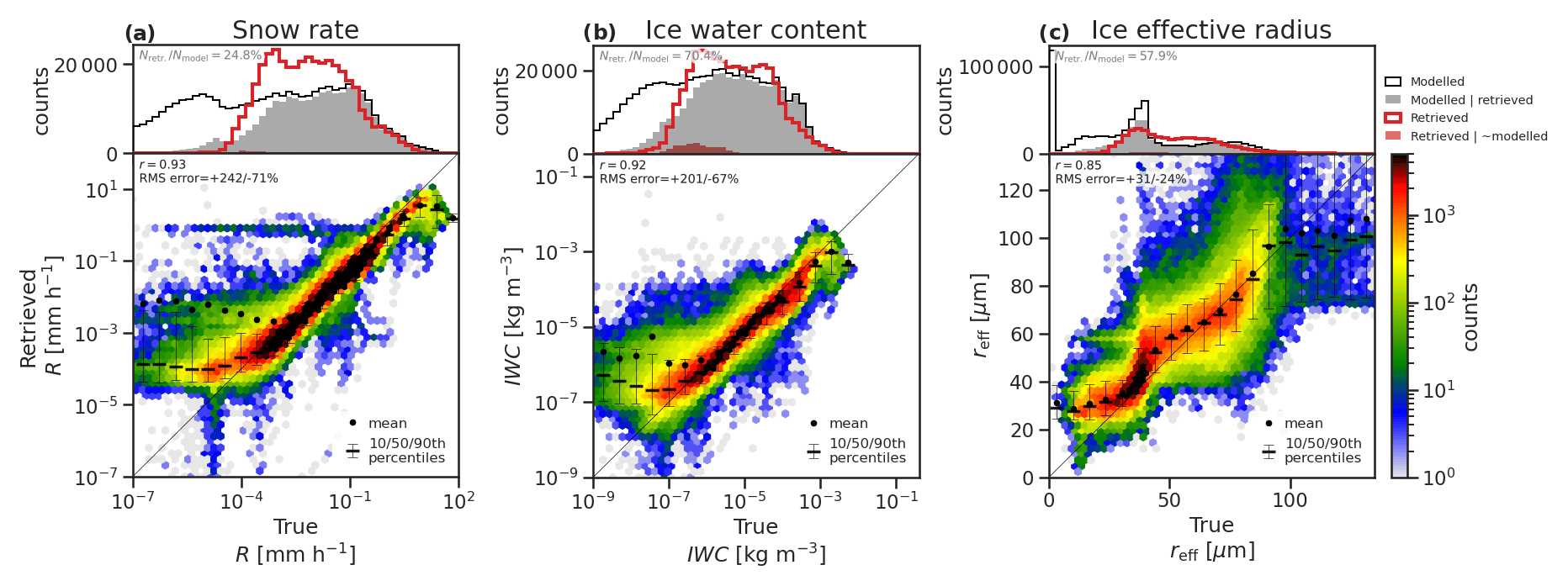
Figure 11 1D (above) and joint (below) histograms comparing true (GEM model) and retrieved (a) snow rate, (b) IWC, and (c) effective radius for the three GEM scenes. The 1D histograms compare all GEM model data (black line) and GEM model data, where ATLID or CPR correctly detect ice cloud (grey shading) against retrieved ACM-CAP data (red line) and retrievals in volumes which do not contain ice cloud (red shading).

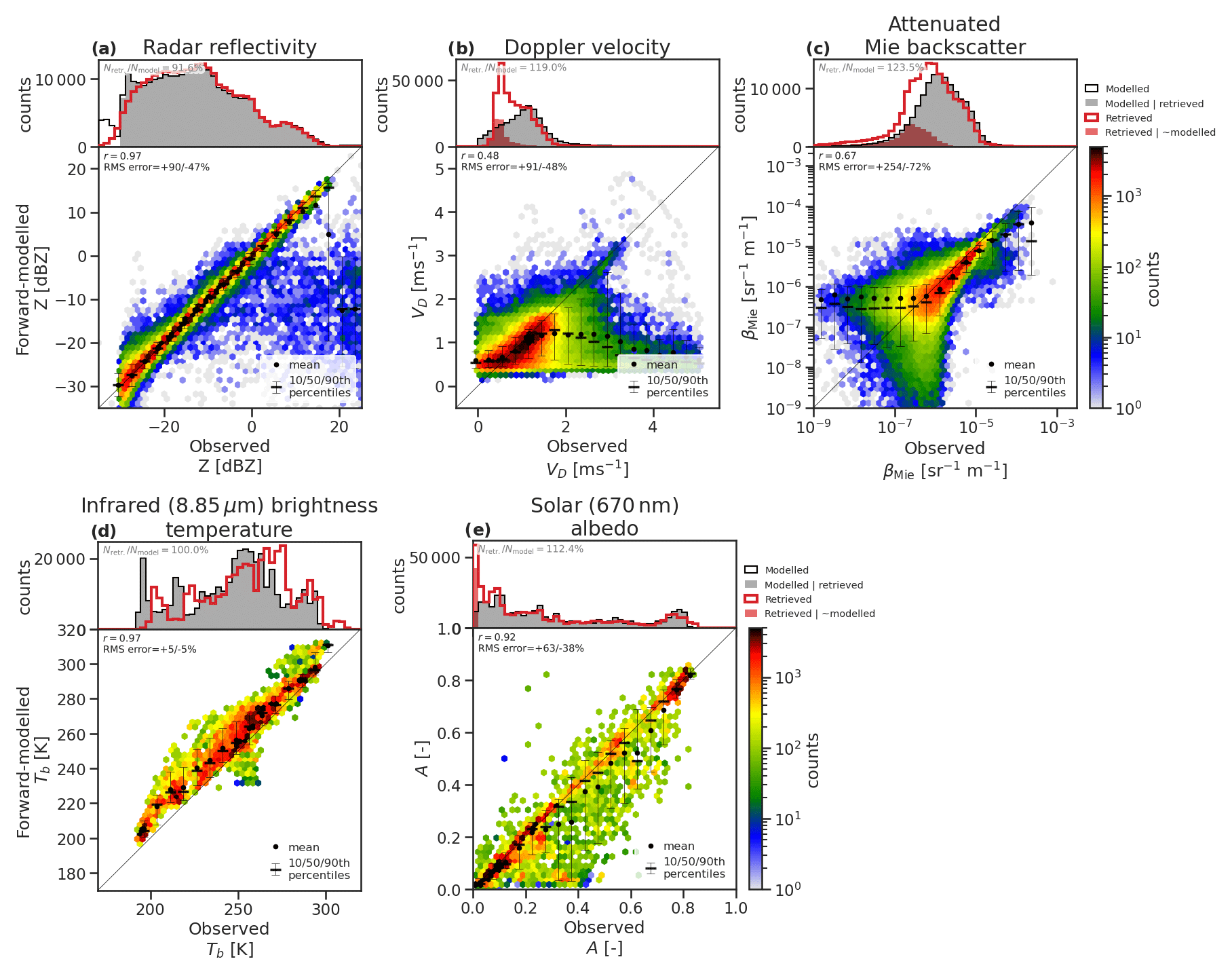
Figure 12 Histograms of observed and forward-modelled CPR radar reflectivity (a), mean Doppler velocity (b), and ATLID attenuated Mie backscatter (c) in volumes containing ice and snow across all three simulated test scenes. The 1D histograms compare all GEM model data (black line) and GEM model data, where ATLID or CPR correctly detect ice cloud (grey shading) against retrieved ACM-CAP data (red line) and retrievals in volumes which do not contain ice cloud (red shading).

The retrieved snow rates (Fig. 11a) and IWC (Fig. 11b) have similar high correlations (r=0.93​​​​​​​ and 0.92) and errors (+242 %/−71 % and +201 %/−67 %); this suggests that the variability in the fall speeds of ice particles – as represented by the numerical model's four ice species – does not dominate the uncertainty in the retrieval. The radar reflectivity is very faithfully reproduced (Fig. 12a) but the mean Doppler velocity (Fig. 12b) – which is well fitted in stratiform snow where the measurement is dominated by the terminal velocity of particles – has a higher degree of spread when the forward-modelled values are less than 1 m s⁻¹, such as in ice clouds dominated by smaller particles.

The GEM model ice effective radius (r_eff) (Fig. 11c) has a bimodal distribution (black line) as an artefact of distinct ice and snow habits in the model microphysics scheme. As ice and snow are represented as a continuum in ACM-CAP, the retrieved distribution of ice effective radius (red line) is only weakly bimodal and shows a tendency to underestimate the frequency of the lowest and highest effective radii. The joint histogram (Fig. 11c) shows that the retrieved effective radius is well-correlated with the GEM model (r=0.85), with low RMS error (+31 %/−24 %); the greater apparent variability in this quantity is due to the linear, rather than logarithmic, scale. The thermal infrared and solar radiances (Fig. 12d, e) both exhibit strong correlations, which is to be expected for passive and integrated measurements that have been assimilated within the retrieval. The warm bias in the infrared brightness temperatures includes a contribution from low IWC near the cloud top being highlighted in parts of the case studies, but – since a similar bias is also evident for the liquid clouds discussed in Sect. 4.2 – we attribute this largely to systematic differences between the atmospheric temperatures in the GEM model and the ECMWF forecasts used to inform the retrieval. By contrast, the shortwave albedo has a higher degree of random error but is not biased.

4.2 Liquid cloud

In this section, we evaluate the retrieved properties of liquid clouds (Fig. 13) and forward-modelled ATLID and MSI measurements (Fig. 14). As shown in the case studies, the retrieval of liquid cloud in rain results in an overall improvement in retrieved LWP, but the smooth spatial distribution of liquid cloud often differs from those in the GEM model (see red shaded PDF in Fig. 13). Overall, the retrieval of liquid clouds is unbiased and moderately correlated with the GEM model variables (r=0.58) but with a high degree of random error (RMSE = +700 %/−87 %).

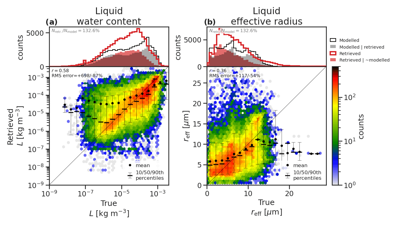
Figure 13 1D (above) and joint (below) histograms comparing true (GEM model) and retrieved (ACM-CAP) liquid water content (left), extinction (middle), and effective radius (right) for the three simulated test scenes. The 1D histograms compare all GEM model data (black line) and GEM model data, where ATLID or CPR correctly detect liquid cloud (grey shading) against retrieved ACM-CAP data (red line) and retrievals in volumes which do not contain liquid cloud (red shading).

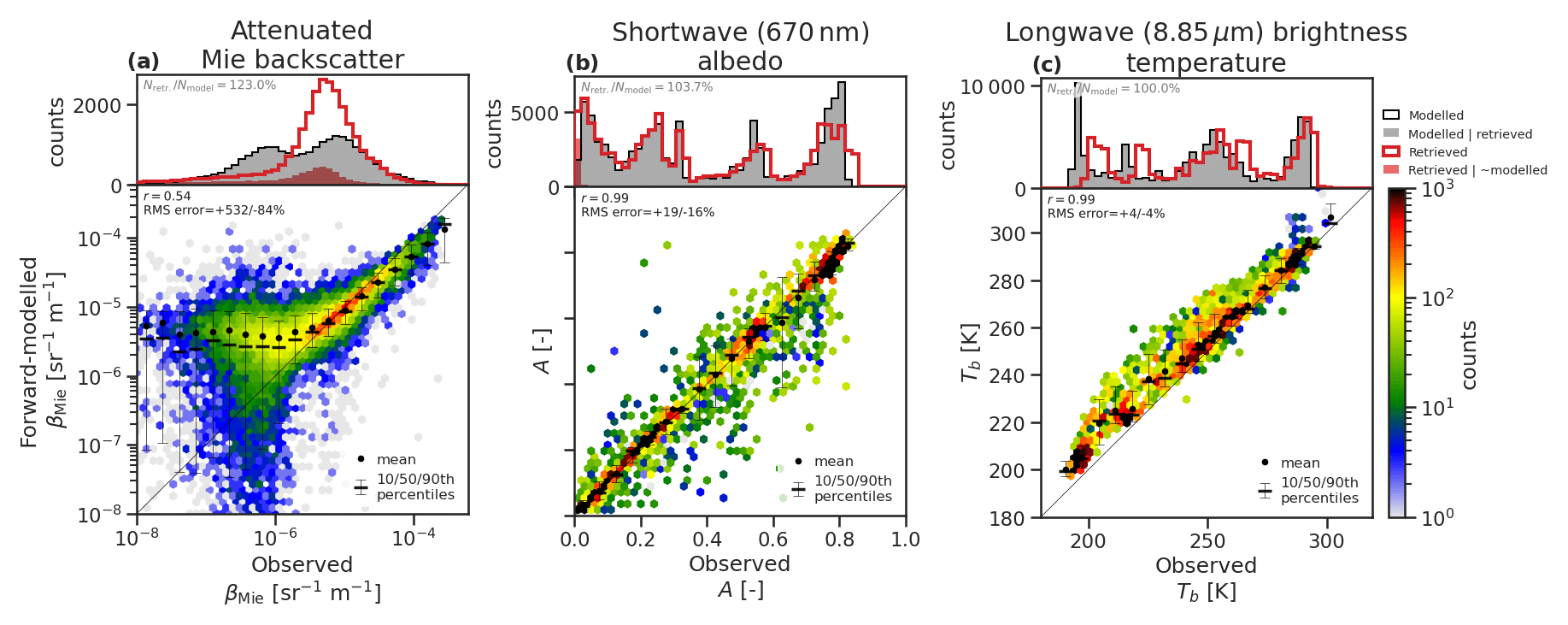
Figure 14 Histograms of observed and forward-modelled ATLID attenuated Mie backscatter (a) and MSI shortwave albedo (b) in volumes and profiles containing liquid cloud across all three simulated test scenes. The 1D histograms compare all GEM model data (black line) and GEM model data where ATLID or CPR correctly detect liquid cloud (grey shading) against retrieved ACM-CAP data (red line) and retrievals in volumes which do not contain liquid cloud (red shading).

The forward-modelled ATLID Mie backscatter and MSI shortwave albedo in liquid clouds (Fig. 14a, b) help evaluate the extent to which the available measurements are correctly assimilated within the retrieval. The attenuated Mie backscatter (Fig. 14a) reflects a moderately good fit to the ATLID measurements; the primary peak in backscatter from liquid clouds around $\mathrm{1}\times {\mathrm{10}}^{-\mathrm{5}}$ sr⁻¹ m⁻¹ is well-represented, but the correlation rapidly deteriorates at lower values (i.e. where the signal is becoming extinguished). The fit to MSI shortwave albedo is extremely good (r=0.99 with RMSE of +19 %/−16 %).

In common with the ice clouds, the MSI thermal infrared (8.85 µm) channel has a warm bias (around 5 K and as much as 10–20 K, especially in higher clouds or colder brightness temperatures) for liquid clouds. A comparison of the temperature fields from the GEM model and X-MET data product derived from the ECMWF analysis revealed temperature differences of as much as several degrees, including positive biases near the cloud top in the three test scenes, which are likely to explain part of the observed bias in MSI thermal infrared channels and which contribute to the uncertainties in this evaluation. In practice, the high-resolution ECMWF 1 d forecasts will also differ from the true state of the atmosphere, but verification against radiosondes reveals that these forecasts have an RMSE of only 1 K in the upper troposphere (Thomas Haiden, personal communication, 2023). Nonetheless, the effect of such errors in the retrieval uncertainty, and the potential for representing these uncertainties within the retrieval, should be the subject of future work.

While the benefit of retrieving liquid cloud in rain was clear from the case studies, it is important that the assumption of liquid cloud in rain can be used at night, without introducing a bias to the retrieval. The high-latitude mixed-phase case study (Fig. 8) showed that ACM-CAP may occasionally underestimate LWP at night, but it is not clear to what extent this would be improved by the availability of solar radiances. As a test, we ran all three scenes without assimilating solar radiances and found that, while LWC exhibited more random error, the retrievals were not biased. This indicates that the priors and uncertainties used are broadly appropriate – at least across the cloud regimes sampled by the test scenes. A more robust check will be to apply the same test using a large number of A-Train orbits.

4.3 Rain

The retrieved properties of rain (Fig. 15) and forward-modelled CPR measurements (Fig. 16) indicate that the rain rate (Fig. 15a) is strongly constrained by radar reflectivity and PIA (Fig. 16a, c) through light to moderate rain rates. A low bias is evident in the heaviest rain (10 mm h⁻¹ and above), corresponding to an underestimate in the highest radar reflectivity factors in rain (above around 15 dBZ). The integrated constraint on attenuation due to both liquid cloud and rain has a correlation of r=0.99 and an RMSE of +49 %/−33 %. In contrast, the mean Doppler velocity (Fig. 16b) and parameters of the raindrop size distribution (DSD; Fig. 15b, c) indicate some challenges in retrieving the microphysics of rain. While mean Doppler velocity has a good correlation with measurements (r=0.67) and a weaker impact from measurement noise than was observed for ice cloud (RMSE = +50 %/−33 %), a low bias is evident in the raindrop terminal velocity, which is reflected in high biases in normalized number concentration and underestimates in median diameter, especially in heavy rain with relatively low concentrations of large raindrops (N_w less than the Marshall–Palmer value and D_m greater than 1 mm). This is likely related to the retrieval being over-constrained by priors when the measurements are near the limits of the CPR within heavy precipitation and may suggest the need to set modified priors for rain within profiles identified as convective.

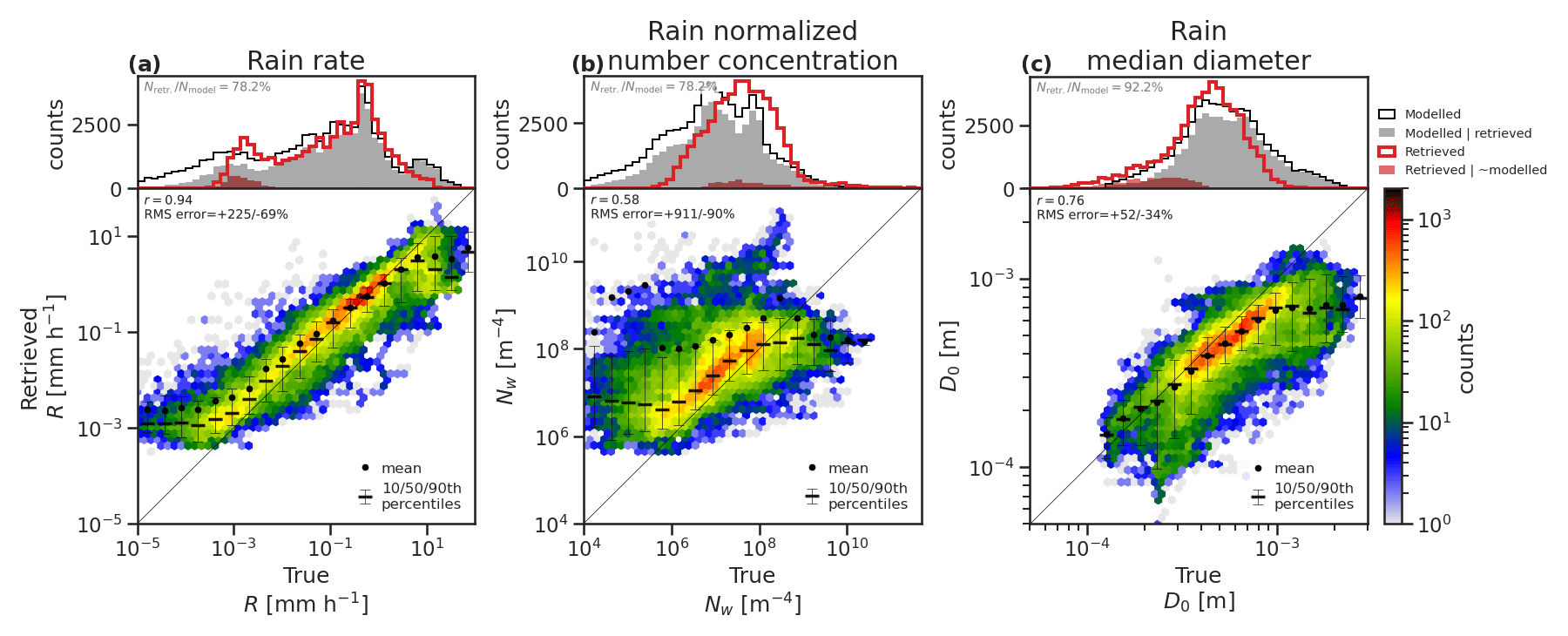
Figure 15 Histograms of GEM model quantities and ACM-CAP retrievals of (a) rain rate, (b) normalized number concentration, and (c) median diameter. 1D (above) and joint (below) histograms comparing true (GEM model) and retrieved (ACM-CAP) rainwater content for the three simulated test scenes. The 1D histograms compare all GEM model data (black line) and GEM model data, where CPR correctly detects rain (grey shading) against retrieved ACM-CAP data (red line) and retrievals in seconds, which do not contain rain (red shading).

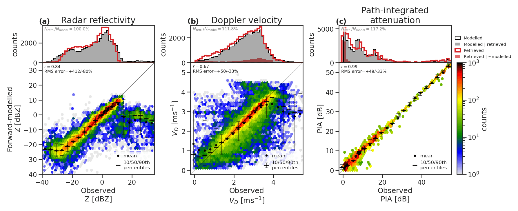
Figure 16 Histograms of observed and forward-modelled CPR radar reflectivity (a), mean Doppler velocity (b), and path-integrated attenuation (c) in seconds and profiles containing rain across all three simulated test scenes. The 1D histograms compare all GEM model data (black line) and GEM model data, where CPR correctly detects rain (grey shading) against retrieved ACM-CAP data (red line) and retrievals in volumes which do not contain rain (red shading).

4.4 Aerosols

The retrieved properties of aerosols and forward-modelled ATLID and MSI measurements (Fig. 18) show that aerosols are the most challenging aspect of the retrieval, given the relatively weak signals and the related issues of characterizing surface properties for the passive measurements. As discussed earlier, the aerosol quantities in the test scenes have been extracted from the CAMS model and mapped to the HETEAC aerosol species in preparation for inclusion in the simulated test scenes (Qu et al., 2022). ACM-CAP relies on the classification of tropospheric aerosols from A-TC to determine the physical properties of each aerosol class, including their scattering properties and size distribution, and retrieves the number concentration by which all other quantities such as extinction and mass content are determined. Hence, there is the quantized distribution of forward-modelled aerosol extinction-to-backscatter ratio, with values corresponding to the properties of each aerosol class (Fig. 17b).

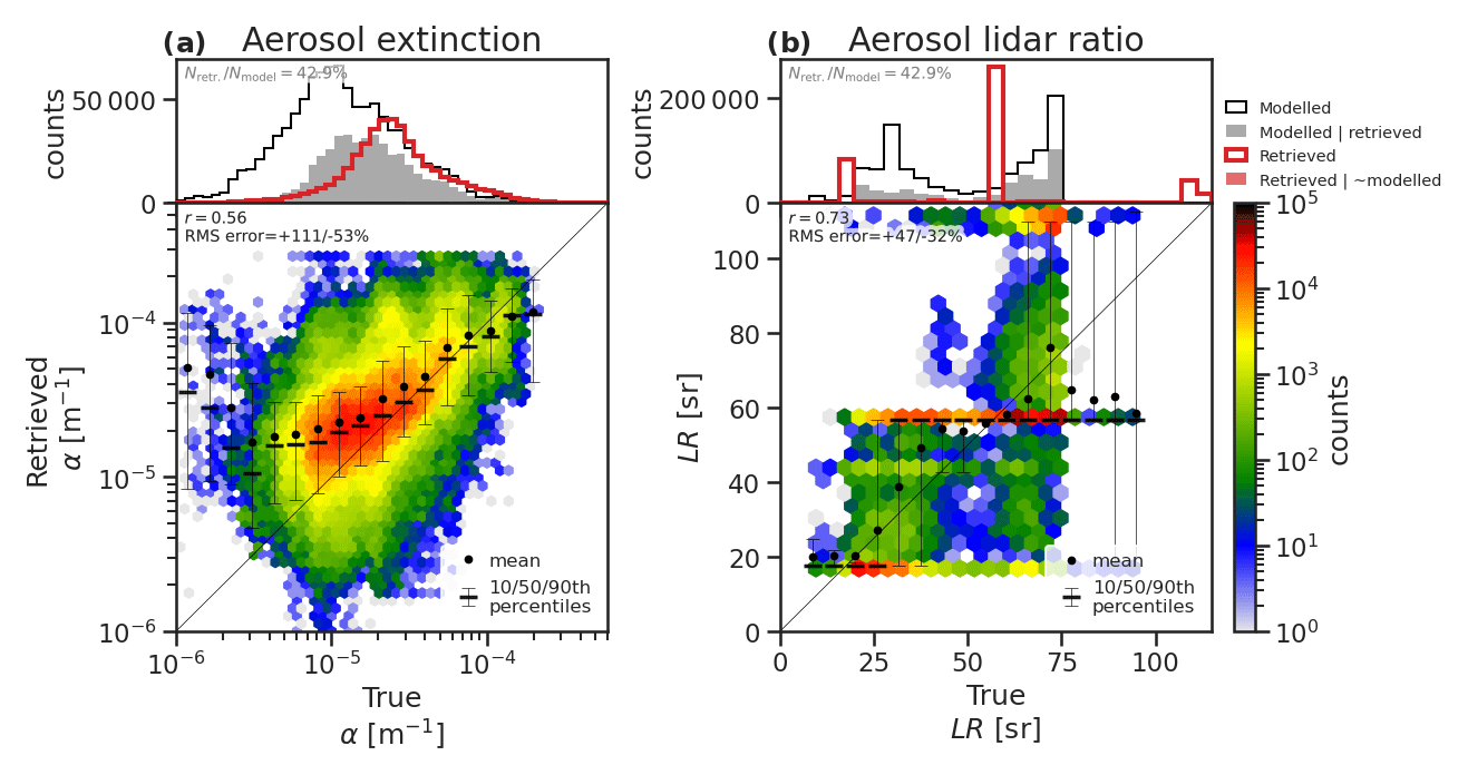
Figure 17 Histograms of CAMS model quantities and ACM-CAP retrievals of (a) aerosol extinction and (b) aerosol lidar ratio (extinction-to-backscatter ratio). 1D (above) and joint (below) histograms comparing true (CAMS model) and retrieved (ACM-CAP) aerosol quantities for the three simulated test scenes. The 1D histograms compare all CAMS model data (black line) and CAMS model data, where ATLID correctly detects rain (grey shading) against retrieved ACM-CAP data (red line) and retrievals in volumes which do not contain rain (red shading).

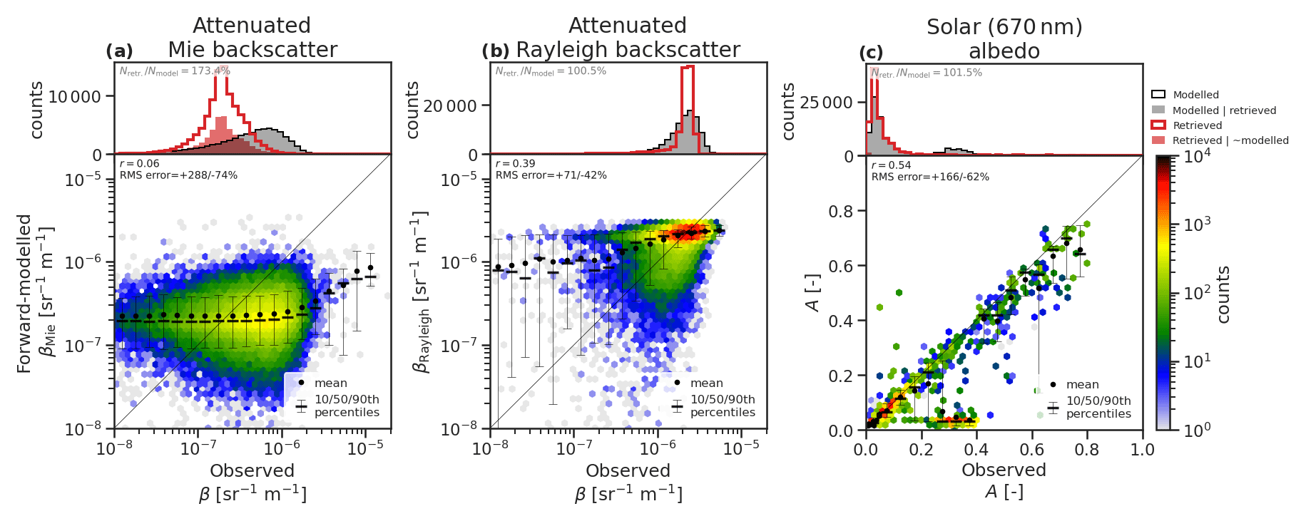
Figure 18 Histograms of observed and forward-modelled (a) ATLID attenuated Mie backscatter, (b) attenuated Rayleigh backscatter, and (c) MSI shortwave albedo in volumes and profiles containing aerosols across all three simulated test scenes. The 1D histograms compare all CAMS model data (black line) and CAMS model data, where ATLID correctly detects aerosols (grey shading) against retrieved ACM-CAP data (red line) and retrievals in volumes which do not contain aerosols (red shading).

The forward-modelled attenuated Mie and Rayleigh backscatter (Fig. 18a, b) have little relation to the measurements at the scale of the JSG. This is consistent with the forward-modelled measurements in the aerosol case study (Fig. 9), where noise dominates the simulated ATLID measurements in the aerosol. This demonstrates the importance of the Kalman smoother for extracting information on larger spatial scales. Errors in the solar albedo appear to be dominated by the land surface (i.e. the Baja scene, crossing North America), with a higher degree of scatter at moderate to high albedos but a relatively close correlation over the ocean (i.e. where A<0.2).

5 Discussion and conclusions

The ACM-CAP product uses the synergy of all available measurements from EarthCARE's active and passive sensors to retrieve profiles of ice and snow, rain, liquid clouds, and aerosols simultaneously. Such a unified retrieval product has never been produced from the synergy of spaceborne instruments and has the advantage of facilitating retrievals, even in mixed-phase, layered, and heavily precipitating scenes. This is a priority for the EarthCARE production model in which the retrievals are used to compute broadband heating rates and inform a top-of-atmosphere radiative closure assessment. In this study, we have described the innovative CAPTIVATE optimal estimation retrieval framework in its configuration for the ACM-CAP processor and presented a detailed evaluation of ACM-CAP's performance across three EarthCARE granules. Taking as truth the numerical model fields used to generate the test scenes, it was possible to evaluate the retrieval more thoroughly than will be possible using in situ or remotely sensed measurements to evaluate in-flight EarthCARE retrievals – with the caveat that the numerical weather model is not a perfect physical representation of aerosols, hydrometeors, or the atmosphere, and some biases in the model may contribute to apparent errors and uncertainties presented here. Over the test scenes, the retrieved IWC and snow rate were closely correlated with the model truth; however, the snow rate was subject to more than twice the random error of IWC, reflecting the high degree of natural variability in the structure and terminal fall speed of snowflakes. The rain retrieval is constrained chiefly by CPR measurements, with important contributions from Doppler velocity and PIA. The retrieved rain rate was very highly correlated with model truth, with a similar random error to that of IWC. Liquid clouds and aerosols are more challenging to retrieve, as both rely on detection by ATLID, which is obscured by cloud aloft and rapidly extinguished in liquid cloud layers. Retrieved LWC was moderately correlated with that in the model, with RMSE around +700 %/−87 %. The retrieved aerosol extinction is moderately correlated with the model but has a lower RMSE of around +110 %/53 %.

The quality of ACM-CAP retrievals is dependent on the accuracy of the target classification used to determine where different species are to be retrieved. A significant limitation of radar-lidar synergy, whether from CloudSat-CALIPSO or EarthCARE, is that of detecting liquid clouds that are either embedded within ice clouds or rain or beneath layered cloud scenes after ATLID is extinguished. An evaluation of the target classifications in the same test scenes (Irbah et al., 2023) showed that liquid cloud is correctly identified by ATLID in around 22 % of sampling volumes – less than 10 % of LWC – and primarily at the tops of mixed-phase clouds and shallow liquid clouds unobscured by optically thick clouds. We have demonstrated a simple assumption to compensate for this missing liquid cloud, which is to assume that liquid cloud is present wherever rain is detected by CPR. While this does not resolve the small-scale structure of liquid clouds within rain, it is sufficient to correctly identify around 54 % of volumes containing liquid cloud or 65 % of LWC (Irbah et al., 2023). We have shown that making the assumption of liquid cloud in rain within ACM-CAP greatly improves the assimilation of MSI solar radiance channels in stratiform rain, constraining the retrieval of a simple profile of LWC. An equally important benefit is that the contribution of liquid cloud to radar attenuation helped to reduce a positive bias in retrieved rain rate in the stratiform precipitation regime. Finally, the fact that liquid cloud in the context of stratiform rain can be coarsely constrained by MSI solar radiance channels suggests its importance for the shortwave broadband fluxes at the top of the atmosphere. The differences between ACM-CAP and other EarthCARE L2 products' retrieved geophysical quantities are explored in an intercomparison study in this special issue (Mason et al., 2023). ACM-CAP's representation of liquid clouds appears to be a contributor to improved shortwave top-of-atmosphere radiative closure when compared to the composite of single-instrument retrievals (Barker et al., 2023).

We have described the configuration of the ACM-CAP retrieval prior to EarthCARE's launch and evaluated its performance, using test scenes generated from a numerical weather prediction model. The test scenes have proved invaluable in facilitating the maturity of the retrieval processor ahead of EarthCARE's launch; however, the three orbital granules represent around 3 % of 1 d of in-flight EarthCARE data and cannot provide a thorough coverage of all the regions and regimes that are of interest for EarthCARE science. Prior to launch, field campaign data, additional simulated scenes, and A-Train data will provide further potential to test and evaluate ACM-CAP, including against in situ measurements of cloud, aerosol, and precipitation properties. Ultimately, the configuration of the ACM-CAP retrieval algorithm will be updated as necessary in response to the exposure of the entire EarthCARE production model to in-flight measurements, in coordination with EarthCARE calibration/validation campaigns.