the Creative Commons Attribution 4.0 License.
the Creative Commons Attribution 4.0 License.
 | 01 Aug 2023
Turbulence kinetic energy dissipation rate: assessment of radar models from comparisons between 1.3 GHz wind profiler radar (WPR) and DataHawk UAV measurements
Lakshmi Kantha
Hiroyuki Hashiguchi
Dale Lawrence
Abhiram Doddi
Tyler Mixa
Masanori Yabuki
The WPR-LQ-7 is a UHF (1.3575 GHz) wind profiler radar used for routine measurements of the lower troposphere at Shigaraki MU Observatory (34.85∘ N, 136.10∘ E; Japan) at a vertical resolution of 100 m and a time resolution of 10 min. Following studies carried out with the 46.5 MHz middle and upper atmosphere (MU) radar (Luce et al., 2018), we tested models used to estimate the rate of turbulence kinetic energy (TKE) dissipation ε from the Doppler spectral width in the altitude range ∼ 0.7 to 4.0 km above sea level (a.s.l.). For this purpose, we compared LQ-7-derived ε using processed data available online (http://www.rish.kyoto-u.ac.jp/radar-group/blr/shigaraki/data/, last access: 24 July 2023) with direct estimates of ε (εU) from DataHawk UAVs. The statistical results reveal the same trends as reported by Luce et al. (2018) with the MU radar, namely (1) the simple formulation based on dimensional analysis , with Lout∼70 m, provides the best statistical agreement with εU. (2) The model εN predicting a σ2N law (N is Brunt–Vaïsälä frequency) for stably stratified conditions tends to overestimate for m2 s−3 and to underestimate for m2 s−3. We also tested a model εS predicting a σ2S law (S is the vertical shear of horizontal wind) supposed to be valid for low Richardson numbers (). From the case study of a turbulent layer produced by a Kelvin–Helmholtz (K–H) instability, we found that εS and are both very consistent with εU, while εN underestimates εU in the core of the turbulent layer where N is minimum. We also applied the Thorpe method from data collected from a nearly simultaneous radiosonde and tested an alternative interpretation of the Thorpe length in terms of the Corrsin length scale defined for weakly stratified turbulence. A statistical analysis showed that εS also provides better statistical agreement with εU and is much less biased than εN. Combining estimates of N and shear from DataHawk and radar data, respectively, a rough estimate of the Richardson number at a vertical resolution of 100 m (Ri100) was obtained. We performed a statistical analysis on the Ri dependence of the models. The main outcome is that εS compares well with εU for low Ri100 (Ri100≲1), while εN fails. varies as εS with Ri100, so that remains the best (and simplest) model in the absence of information on Ri. Also, σ appears to vary as when Ri100≳0.4 and shows a degree of dependence on S100 (vertical shear at a vertical resolution of 100 m) otherwise.
- Article
(1600 KB) - Full-text XML
- BibTeX
- EndNote


The dissipation rate ε (m2 s−3 or W kg−1) of turbulence kinetic energy (TKE) is an important variable for assessing the rate of change of TKE with time. This variable appears in a simplified expression of the ensemble-mean TKE budget equation (see, e.g., Stull, 1988, for a complete derivation and for its conditions of validity):
where P is the shear production term and B the buoyancy flux term. Note that advection terms on the left-hand side have been omitted. Under steady-state conditions, the left-hand side is zero, and there exists a balance between the rates of shear production, buoyancy production/dissipation and dissipation of TKE. In practice, ε can be estimated in the atmosphere from VHF stratosphere–troposphere radar and UHF wind profiler measurements of Doppler spectral width, hereafter, noted 2σobs (m s−1) (e.g., Hocking, 1983, 1985, 1986, 1999; Fukao et al., 1994; Cohn, 1995, Kurosaki et al., 1996; Bertin et al., 1997; Delage et al., 1997; Naström and Eaton, 1997; Dole et al., 2001; Jacoby-Kaoly et al., 2002; Satheesan and Krishna Murthy, 2002; Naström and Eaton, 2005; Wilson et al., 2005; Kalapureddy et al., 2007; Singh et al., 2008; Dehghan and Hocking, 2011; Kantha and Hocking, 2011; Dehghan et al., 2014; Wilson et al., 2014; Hocking et al., 2016; Li et al., 2016; Kohma et al., 2019; Jaiswal et al., 2020; Chen et al., 2022).
Several models have been proposed to relate 2σobs to ε. Some studies have accepted the validity of these models in order to perform statistical analyses of the turbulence characteristics in the troposphere–stratosphere (e.g., Fukao et al., 1994; Kurosaki et al., 1996; Naström and Eaton, 1997; Kalapureddy et al., 2007; Fukao et al., 2011; Chen et al., 2022). Other studies have tested the consistency between models based on spectral width measurement and their consistency with other radar models based on echo power or radial wind velocity variance measurement (e.g., Cohn, 1995; Bertin et al., 1997; Delage et al., 1997; Satheesan and Krishna Murty, 2002; Singh et al., 2008). Yet others assessed the radar estimates from cross-comparisons with indirect estimates based on the Thorpe sorting method applied to potential temperature profiles measured by standard radiosondes (e.g., Clayson and Kantha, 2008; Kantha, 2010; Kantha and Hocking, 2011; Wilson et al., 2014; Li et al., 2016; Kohma et al., 2019; Jaiswal et al., 2020). However, attempts at validations from direct in situ estimates of ε from velocity fluctuation measurements remain very rare. McCaffrey et al. (2017) compared ε estimates derived from a UHF wind profiler and those obtained from sonic anemometer energy spectra made at a 300 m altitude. Shaw and LeMone (2003) and Jacoby-Koaly et al. (2002) evaluated the performance of UHF wind profilers from in situ ε aircraft and/or tower measurements mainly in the convective boundary layer. Dehghan et al. (2014) made ε comparisons between aircraft and the VHF (40.68 MHz) Harrow radar with mixed results.
In addition to being rare, the above-mentioned studies did not aim to test the same radar models. Luce et al. (2018), hereafter denoted L18, assessed different models from comparisons with direct estimates of ε from air speed fluctuation measurements made from highly sensitive Pitot sensors aboard DataHawk UAVs and the VHF 46.5 MHz middle and upper atmosphere (MU) radar observations in the lower troposphere. One of the objectives of the present work is to show that the conclusions obtained from comparisons with the MU radar are also quantitatively valid for the WPR-LQ-7 (Imai et al., 2007), a UHF wind profiler routinely used at the Shigaraki MU Observatory. We also introduce and test another model expected to be valid for weakly stratified or strongly sheared conditions, i.e., low Richardson (Ri) numbers (Hunt et al., 1988; Basu et al., 2021; Basu and Holtslag, 2021) for which the static stability effects can be ignored. Ri is defined as , where is the squared Brunt–Väisälä frequency (s−2), g≈9.81 m s−2 is the gravitational acceleration, θ (K) is the potential temperature and S (s−1) is the vertical shear of the horizontal wind vector.
Section 2 introduces the expressions for ε used in the present paper with a focus on the newly introduced model in radar studies. Section 3 briefly describes the WPR-LQ-7 and the methods used for the comparisons. Section 4 describes the results for two turbulent layers, one of which was clearly produced by a Kelvin–Helmholtz (K–H; shear flow) instability because of the observation of S-shaped structures specific to this instability in both time–height MU and WPR-LQ-7 echo power cross-sections. The results of comparisons of ε values obtained from the different models applied to the two radars, DataHawk measurements, and a simultaneous radiosonde using the Thorpe sorting method of vertical potential temperature profiles are described for the two layers. Section 5 shows statistics on the consistency between the estimates of ε from the different models and the DataHawks and describes the dependence of the models on Ri. Finally, conclusions are given in Sect. 6.
2.1 The models tested by L18
The different models and their conditions of application have already been described by L18. Here, the expressions are simply reintroduced. Assuming a vertically pointing radar beam, the first expression is
where σ2 is an estimate of the variance 〈w′2〉 of the vertical wind fluctuations produced by turbulence. Lout has the dimension of a length scale and represents the scale of energy containing turbulent eddies if σ2 is an unbiased estimate of 〈w′2〉. In practice, σ2 is obtained after removing the non-turbulent contributions from (e.g., Hocking, 1983; Nastrom, 1997; Hocking et al., 2016, and references therein). The practical method used in the present work is described in the Appendix of L18. The dissipation rate is expected to vary as σ3 if σ and Lout are independent or when the typical scale of turbulent eddies exceeds the dimensions of the radar volume, so that Lout would mainly be a function of these dimensions (e.g., Frisch and Clifford, 1974; Labitt, 1979; Doviak and Zrnić, 1984; White et al., 1999).
The second expression (e.g., Hocking, 1983, 1999; Hocking et al., 2016) is
where CN is a constant. This expression is expected to be valid for turbulence in a stable stratification (N2>0) whose outer scale is defined by the buoyancy length scale expressed as . Equation (3) is thus equivalent to . In a pioneering contribution, Hocking (1983) first derived Eq. (3) from the integration of the transverse 1D spectrum of vertical velocities over the inertial and buoyancy subranges to relate ε to 〈w′2〉. In its original derivation, the author assumed roughly equal contributions to 〈w′2〉 from the inertial and buoyancy subranges. More recently, Hocking et al. (2016) proposed a more general expression by introducing a variable factor F, where F is the ratio of the buoyancy contribution to the inertial subrange contribution. This factor can vary from 0.5 to 1. It affects the value of the constant CN, and Hocking et al. (2016) recommend that a value of (0.5±0.25) be used, which takes into account the variability of F, which is difficult to determine in practice.
The results of comparisons using Eqs. (2) and (3) reported by L18 with DataHawk-derived ε showed that Eq. (2) provides the best overall statistical comparisons for Lout∼ 50–70 m. On the other hand, the analysis of the comparison results with εN suggested that N is not a key parameter since the quality of the comparisons appeared to be independent of N.
2.2 The model for strongly sheared or/and weakly stratified flows
While it seems that the conditions of strong shear and weak stratification have not received much attention in the radar community, several studies showed that ε can be written as (Hunt et al., 1988; Schumann and Gerz, 1995)
Note that we do not make the distinction between σ2 and 〈w′2〉 for simplicity. Equation (4) is equivalent to , where is the Hunt length scale. Equation (4) can be interpreted as the fact that turbulent eddies are first stretched by shear before being affected by stratification in strongly sheared or weakly stratified flows. This concept was discussed by Hocking and Hamza (1997), but they did not mention the Hunt length scale and did not go further into it. Hunt et al. (1988) suggested that Eq. (4) can be valid up to Ri∼0.5. Schumann and Gerz (1995) even proposed up to Ri∼1 from large eddy simulations. Hunt et al. (1988) proposed CS≈0.45 for neutral stationary boundary layers. Kaltenbach et al. (1994) found from large eddy simulations. By using Eq. (1) for a homogeneous shear layer in steady state, i.e., , and similarity theory, Basu and Holtslag (2021) re-evaluated the constant CS and provided a generalization of Eq. (4):
with CS=0.63. Rf is the flux Richardson number. It is related to the turbulent Prandtl number Pr by . Basu et al. (2021) found from direct numerical simulation (DNS) that Eq. (4) with CS∼0.60 is valid up to Ri∼0.2 at least. For , decreases from 0.63 to 0.60, using the analytical expression (Eq. 22) of Basu and Holtslag (2021) for Pr(Ri). For Ri→0, we have Rf→0, then . For Ri→1, Rf∼0.25, . Therefore, Eq. (3) would be quantitatively equivalent to Eq. (5a) for Ri of the order of 1 despite the fact that the two approaches cannot be reconciled because, in essence, there is no contribution from an anisotropic buoyancy subrange in Eq. (5a). Equation (4) removes an inconsistency in Eq. (3), since it wrongly indicates that ε→0 when N→0 for a given σ2. If S=0, i.e., if the source of the instability that generates turbulence is removed, then ε=0, which makes more sense.
As discussed by Basu and Holtslag (2021, Sect. 6.2) and Basu and Holtslag (2022, their Appendix 1), the derivation of Eq. (5) does not consider the fact that the steady-state condition (also called “full equilibrium” (FE), Baumert and Peters, 2000) can only be reached for a single value of Richardson number Ris, at least for large Reynolds numbers and large shear parameters STL, where TL is the inertial timescale defined as (see, e.g., Mater and Venayagamoorthy, 2014). For Ri<Ris, TKE increases at subcritical Ri, and for Ri>Ris, TKE decreases (turbulence decays) at supercritical Ri (e.g Baumert and Peters, 2000). From large eddy simulation (LES) and DNS data, Schumann (1994) and Gerz et al. (1989) reported RiS≈0.13 for air, consistent with the value that can be deduced from Fig. 1 of Mater and Venayagamoorthy (2014). Schumann (1994) re-wrote the TKE budget Eq. (1) as where is called the growth factor. G=1 for FE conditions. By assuming, for simplicity, that G only depends on Ri, Schumann proposed the empirical expression with based on wind-tunnel data analysis. By using the same procedure as Basu and Holtslag (2021) from their Eqs. (10) to (12) but starting with , we get
Equation (5b) can also be directly obtained by using Eq. (46a) in Eq. (10b) of Basu and Holtslag (2021). For , increases from 0.52 to 0.70, i.e., ∼0.60 on average, for Ris≈0.13 and G0=1.47. The Ri dependence of is thus only a small source of dispersion for low Ri values when comparing with other estimates.
From the results of Baumert and Peters (2000) using a “structural equilibrium” approach (i.e., stationarity of ratios of turbulence characteristics) and based on laboratory and LES data (their Fig. 4), we can establish εS=0.15σ2S valid for Ri≲0.25. This expression is obtained by combining , and , where and are the Ellison and Ozmidov length scales, respectively. The constant differs very significantly (by a factor of 3 to 4 less) from the aforementioned estimates. If we use as proposed by Schumann (1994) for Ri≤0.25, we get εS=0.44σ2S with the same ratio. These expressions are more subject to experimental uncertainties and are thus not considered in this paper. In Appendix A, we propose an alternative derivation of Eq. (4), suggesting . We retain the value of CS=0.63 for the comparisons between the models.
Following the spectral approach proposed by Weinstock (1981), Eq. (4) with CS equal to CN≈0.5 can also be obtained from the integration of the 1D Kolmogorov ( slope) scalar kinetic energy spectrum over a spherical shell of radius kH instead of kB, where kH(kB) is the wavenumber corresponding to LH(LB). For the context of radar measurements (e.g., Hocking et al., 2016), Eq. (4) can also be obtained from the integration of the 1D transverse vertical velocity spectrum with a slope for large (horizontal) wavenumbers (k>kH) and a zero slope for (k<kH), both mathematical developments being equivalent.
Finally, εS has the advantage that it can be evaluated entirely from the radar data, since the wind shear S can be estimated at the range and time resolutions of the radar, unlike εN which requires N2 to be obtained from in situ or radio-acoustic sounding system measurements.
3.1 The WPR-LQ-7
The WPR-LQ-7 is a 1.3575 GHz Doppler radar. It has a phased array antenna composed of seven Luneberg lenses of 800 mm diameter. Its peak output power is 2.8 kW. It can be steered into five directions sequentially (i.e., after fast Fourier transform (FFT) operations), vertical and 14.2∘ off zenith toward north, east, south and west. The main radar parameters of the WPR-LQ-7 installed at Shigaraki MU Observatory since 2006 are given in Table 1.
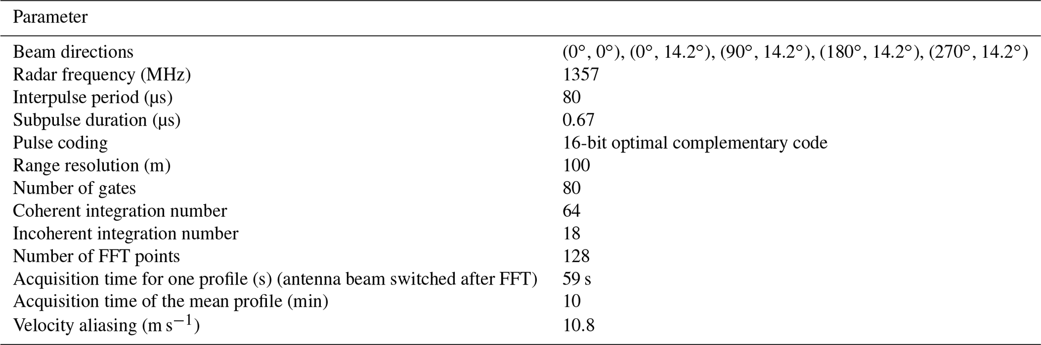
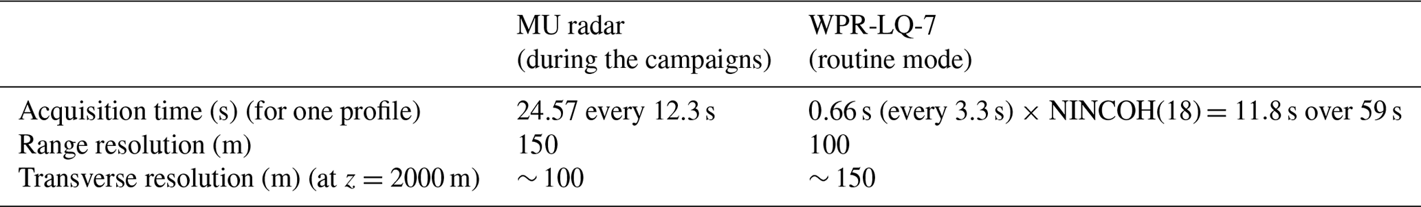
The acquisition time for one profile composed of 80 altitudes from 300 m a.g.l. (∼ 684 m a.s.l.) every 100 m in each direction is 59 s after 18 incoherent integrations but for a total of 11.8 s of observations for each direction (due to the intertwining between the directions). The time series are processed by automatic algorithms to remove outliers (e.g., bats, birds, airplanes) and ground clutter as far as possible. Low signals near and below the detection thresholds are removed, and profiles of atmospheric parameters (echo power, radial winds, half-power spectral width, horizontal and vertical winds) averaged over 10 min are made available for routine monitoring (http://www.rish.kyoto-u.ac.jp/radar-group/blr/shigaraki/data/, last access: 24 July 2023). Because of the high data quality control, the 10 min averaged data are used to retrieve ε with the objective to assess the routine data for further analysis. The 59 s resolution data and those collected by the MU radar at a time resolution (sampling) of 24.57 s (∼ 12.3 s) were used to help identify atmospheric structures from height–time signal-to-noise ratio (SNR) or echo power cross-sections, such as convective cells or Kelvin–Helmholtz (K–H) billows. Table 2 shows the acquisition time, the range and transverse resolutions of the WPR-LQ-7 for the altitude range of comparisons, and the range and resolutions of the MU radar for the data used in the present work.
Table 2Time, range and transverse resolutions of the MU radar and WPR-LQ-7 for the dataset used in the present work. NINCOH refers to the number of incoherent integrations. The range resolution is , where c is the light speed and τ is the pulse duration, and the transverse resolution is 2θ0z, where θ0 is the half-power half width of the effective (two-way) radar beam and z is the altitude as defined in L18. The time series of MU radar signals are weighted by a Hanning window before FFT calculations.
3.2 The methods of comparison with DataHawk-derived ε
The DataHawk datasets were collected during two field campaigns, called the Shigaraki UAV Radar Experiment (ShUREX), in May–June 2016 and June 2017 at the Shigaraki MU observatory. The DataHawks were flying about 1 km away from the MU radar and the WPR-LQ-7. Kantha et al. (2017) described the instruments and configurations used during a previous ShUREX campaign in June 2015. The processing method used to retrieve ε from Pitot sensor data is not recalled here as it is described in detail by L18 for comparisons with MU radar data. The trajectories of the DataHawks being helicoidal upwards or downwards, pseudo-vertical profiles of ε at a vertical sampling of ∼ 5 m typically were obtained during the ascents and descents of the aircraft, from the ground up to a maximum altitude of ∼ 4.5 km. A total of 36 DataHawk datasets collected during the two campaigns provided 90 full or partial profiles used for the comparisons. Section 4 describes one of these flights with one full ascent (A1) and descent (D2) and one partial ascent (A2) and descent (D1). Three DataHawk flights collected during periods of precipitation contaminating the WPR-LQ-7 returns were rejected. The DataHawk-derived ε profiles were smoothed with a Gaussian window and resampled at the altitude of the radar gates to simulate the radar range resolution. The degraded DataHawk 100 m resolution profiles are hereafter denoted εU.
The WPR-LQ-7-derived , εN and εS profiles were computed at a time resolution of 10 to 30 min, i.e., by averaging up to three consecutive profiles that best correspond to each period of DataHawk ascent or descent. was calculated with Lout=70 m in accordance with the best agreement from comparisons with the MU radar (L18) and the statistics of Lout shown in Sect. 5. The profiles of N2 at a vertical resolution of 100 m were estimated from pressure and temperature profiles collected by the DataHawks. These profiles were used to obtain εN (Eq. 3). εS profiles were computed from Eq. (4) every 10 min from wind shear estimated from radar data and then averaged up to 30 min.
3.3 Estimation of ε from the Thorpe method applied to radiosonde data
The Ozmidov length scale is commonly assumed to be proportional to the Thorpe length , where d′ is the Thorpe displacement in the so-called Thorpe layer. Then, we have LO=cLT and
The literature is very divided on the value of c to use (see Kohma et al., 2019, for a review). Wijesekera and Dillon (1997) showed large temporal variations of from observations in the ocean. Large temporal variations were also reported from DNS depending on the stage and source of turbulence (e.g., Fritts et al., 2016). An intermediate value of c=1 is sometimes used by default (e.g., Kantha and Hocking, 2011). However, Mater et al. (2013) showed that c∼1 when the turbulent Froude number is near unity (at the transition between shear- and buoyancy-dominated regimes). The basic N2 for the Thorpe layers is generally estimated from the sorted potential temperature profile or from the rms value of the fluctuations defined as the difference between the measured and sorted profiles (e.g., Smyth et al., 2001; Wilson et al., 2014).
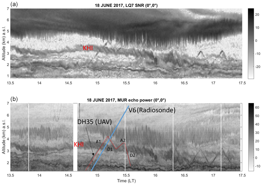
Figure 1(a) Time–height cross-section of WPR-LQ-7 signal-to-noise ratio (dB) at vertical incidence on 18 June 2017 from 13:30 to 17:30 LT. (b) The corresponding time–height cross-section of MU radar echo power (dB) in (high-resolution) range imaging mode at vertical incidence. “A1”, “D1”, “A2” and “D2” refer to the consecutive ascents and descents of the DataHawk UAV (DH35), emphasized by the red lines. The blue line shows the time–altitude of the radiosonde V6 launched at 14:51 LT from Shigaraki MU Observatory.
Another scale, called the Corrsin length scale, is defined as . It is the counterpart of the Ozmidov length scale for shear flows under neutral stratification conditions. Similarly, assuming , we can write
Equation (7) is thus a possible alternative to Eq. (6), when the Corrsin length scale is smaller than the Ozmidov length scale. These equations are coherent with the results of Mater et al. (2013), who showed that LT scales with in the shear-dominated regime and with in the buoyancy-dominated regime. Equation (7) can also be justified, and the parameter c′ can be estimated as follows. The aforementioned ratios and , found for weakly stratified flows (Ri≤0.25) by Baumert and Peters (2000) and Schumann (1994), respectively, may be representative of for flows free of gravity wave motions. Indeed, LE=LT is obtained if is a constant, which implies the absence of gravity waves. By introducing the expressions of into Eq. (6), we obtain Eq. (7), with c′ (hereafter noted ) equal to or c′ (hereafter noted ) equal to . Note that c′ is a constant, while c depends on Ri. For a shear-dominated regime, from Fig. 3e, f, g and h of Mater and Venayagamoorthy (2014), we can typically deduce from DNS and from experimental data, which is very consistent with the other values. In Appendix B, we show that can be found from an alternative approach based on the inference of the turbulent Froude number from for weakly stratified flow condition (Garanaik and Venayagamoorthy, 2019).
Equations (6) and (7) are equivalent if Eq. (5) is written as
Equations (4) and (7) have in common that they are formally independent of N2 when Ri≲0.25. If they were both to be confirmed by experimental analysis, they would constitute a coherent whole.
Figure 1a shows the time–height cross-section of WPR-LQ-7 SNR (dB) at vertical incidence and a time and range resolution of 59 s and 100 m, respectively, on 18 June 2017 from 13:30 to 17:30 LT and in the altitude range [0.685–7.0 km] a.s.l. (a.s.l. = a.g.l. + 0.385 km). Figure 1b shows the corresponding cross-section of MU radar echo power (dB) at vertical incidence and a time resolution of ∼12 s after doing range imaging with Capon processing (e.g., Luce et al., 2017) in the altitude range [1.275–7.0 km]. Radar echoes from a DataHawk, called “DH35” in reference to the flight numbering, are visible after ∼ 14:30 and before ∼ 15:40 LT on both images. They are the signatures of two ascents (“A1”, “A2”) and two descents (“D1”, “D2”) of a DataHawk. Four red segments emphasize them in Fig. 1b. Incidentally, radar echoes from another DataHawk (DH36) can be noted after 16:30 LT. A Vaisala RS92-SGP radiosonde, called “V6”, was launched at 14:51 LT from the observatory. Its time–height position is indicated by the blue line in Fig. 1b. It roughly coincides with A1.
An approximately 800 m deep enhanced echo power layer with S-shaped structures, signature of Kelvin–Helmholtz billows, is clearly visible in both images in the altitude range [3.0–4.0 km] until ∼ 16:00 LT at least. The layer is denoted by “KHI” on the images. DH35 crossed the layer four times during A1, D1, A2 and D2 between 15:00 and 15:30 LT. DH35 sampled the most obvious case of K–H instability during the entire two campaigns. Since a necessary condition for the development of K–H billows is at the critical level, their observation suggests that it was fulfilled when sampled by the instruments. Another focus will be given to a turbulent layer between 2100 and 2500 m, sampled twice by DH35 during A1 and D2, even though it is not clearly visible in the radar echo power images (Fig. 1). For this layer, Ri is expected to be ≳1 according to various estimates and layer properties described in Sect. 4.2.
The analysis of these two cases is done to illustrate the differences in the ε behavior of the three different radar models applied to two radars, possibly at different Richardson numbers (Ri≲0.25 and ≳1), compared to the DataHawk-derived ε.
4.1 The K–H layer
4.1.1 Comparisons between DataHawk-derived ε, , εN and εS
Figure 2a shows the four DataHawk-derived ε profiles during A1, D1, A2 and D2 (dotted black lines) and the profiles of , εN and εS in the height range [2000–3900] m obtained from the WPR-LQ-7 data (solid red, blue and green lines, respectively) and MU radar data (dashed red, blue and green lines, respectively). Figure 3a, b and c show the same information for the three models but separately. For clarity, because they are virtually identical during D1, A2 and D2, the radar-derived ε profiles are shown for A1 (15:00–15:20 LT) only. The sources of errors and uncertainties on radar estimates are multiple (e.g., Dehghan and Hocking, 2011), and confidence intervals for each individual estimate are difficult or even impossible to establish. However, the consistency between the estimates from successive independent segments of data and concordant temporal evolution as shown in Fig. 4 and Table 3 gives some credence to the significance of the comparisons. Table 3a and the corresponding figure, Fig. 4, show ε, , εN and εS values averaged over the depth of the K–H layer for A1, D1, A2 and D2. The DataHawk-derived ε values peak in the range of the K–H layer and vary little during the ascents and descents over ∼ 30 min: typically ∼ 2 mW kg−1. During A1, the DataHawk-derived ε profile shows a narrower peak between 3200 and 3600 m. The DataHawk may have sampled a thinner region of the K–H layer (∼400 m), perhaps associated with the edge of a K–H billow. This could also be the case for V6 as the Thorpe analysis suggests a ∼300 m deep layer at the altitude of ∼3.3 km (and an additional thinner layer around the altitude of ∼3.6 km). If we exclude the difference in layer depth during A1, and εS estimated from both radars coincide very well with DataHawk-derived ε both in shape and levels during A1, D1, A2 and D2, with very similar variations in time (Table 3a and Fig. 4), indicating that the two radar models are satisfactory and are equivalent in these circumstances. In contrast, the εN profiles exhibit the worst agreement with DataHawk-derived ε near the center of the K–H layer where they show a minimum (Figs. 2a and 3b, solid and dashed blue lines). This feature is similar to the one reported by L18 (their Fig. 12) for a turbulent layer generated by a convective instability at a mid-level cloud base. Table 3a and Fig. 4 confirm that 〈εN〉 values are lower than the other estimates by a factor of 2 to 3 approximately during A1, D1, A2 and D2 for both radars. This disagreement, occurring repeatedly on the two radars, confirms the inadequacy of the εN model for this layer.
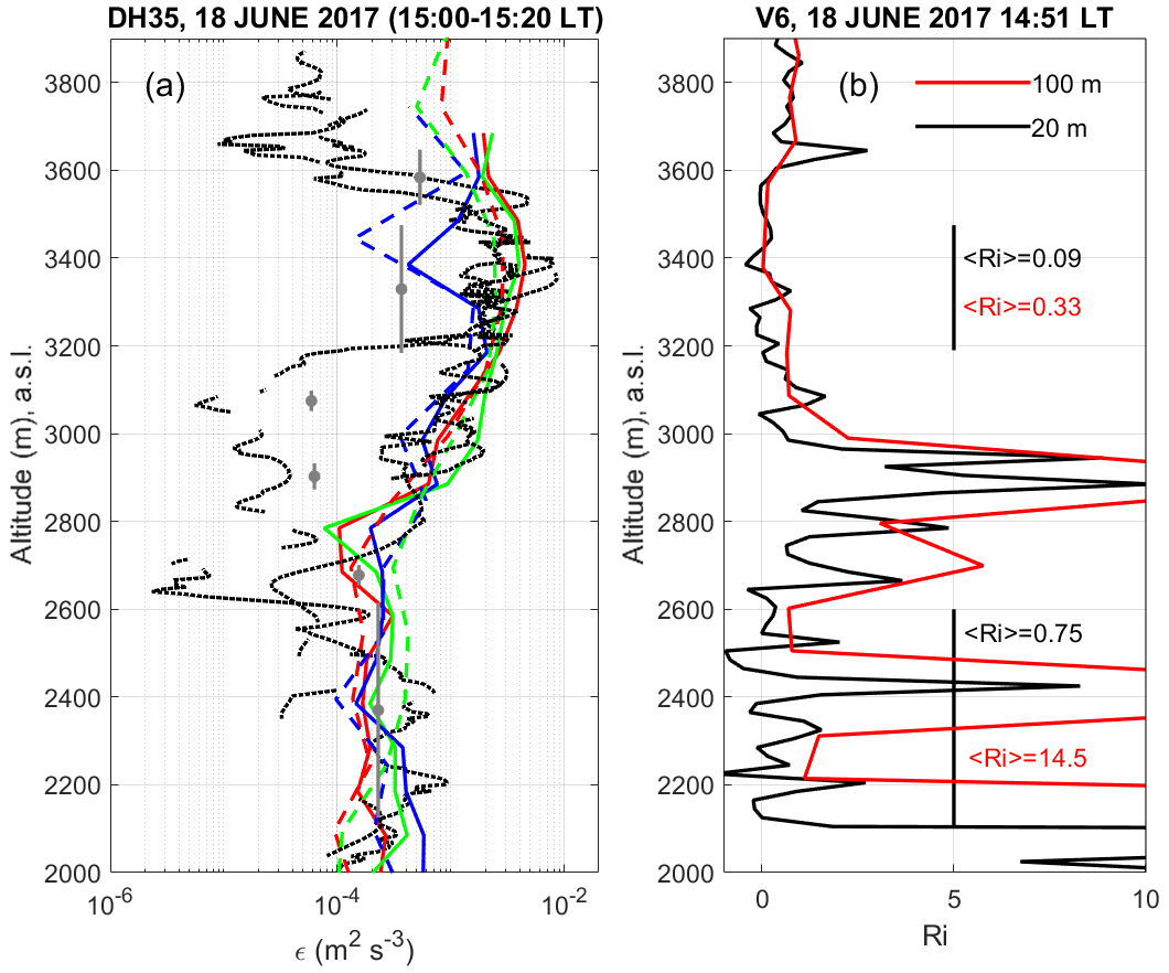
Figure 2(a) DataHawk-derived ε (m2 s−3) profiles in the height range [2000–3900] m during A1, D1, A2 and D2 of DH35 on 18 June 2017 (dotted black), εS(LQ-7) profile (solid red), profile (solid green), εN(LQ-7) profile (solid blue), εS(MU) profile (dashed red), profile (dashed green) and εS(MU) profile (dashed blue) derived from radar data between 15:00 and 15:20 LT. Grey dots and lines show εT (Eq. 6) with c=1, the depth and altitude of the Thorpe layers. (b) Richardson number profiles estimated from RS92-SGP Vaisala radiosonde V6 data at a vertical resolution of 20 m (black) and 100 m (red).
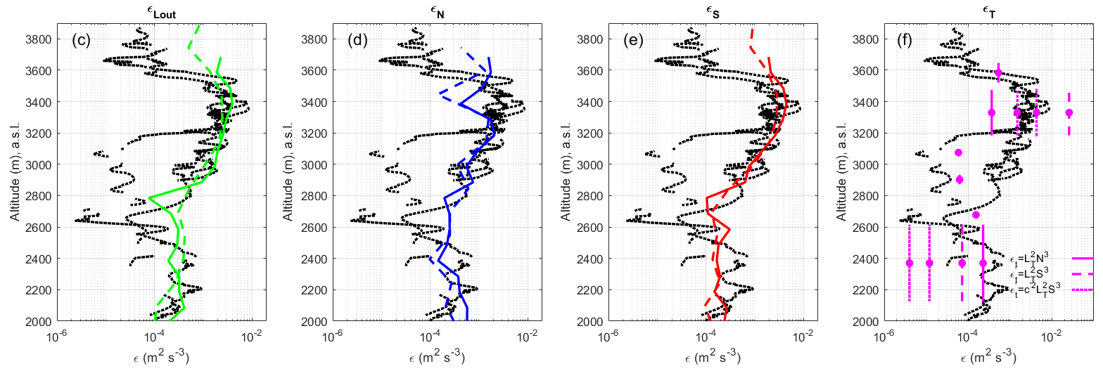
Figure 3Same as Fig. 2a but with separate plots for each model: (a) , (b) εN, (c) εS and (d) εT, respectively. Panel (d) shows the results in magenta for εT (Eq. 6) with c=1 (solid line), (Eq. 7) with (dashed line), and (Eq. 7) with and (dotted line).
Table 3Mean values of TKE dissipation rates (mW kg−1) according to the different models and instruments for the K–H layer (a) and for the turbulent layer (TL) between 2100 and 2500 m (b).
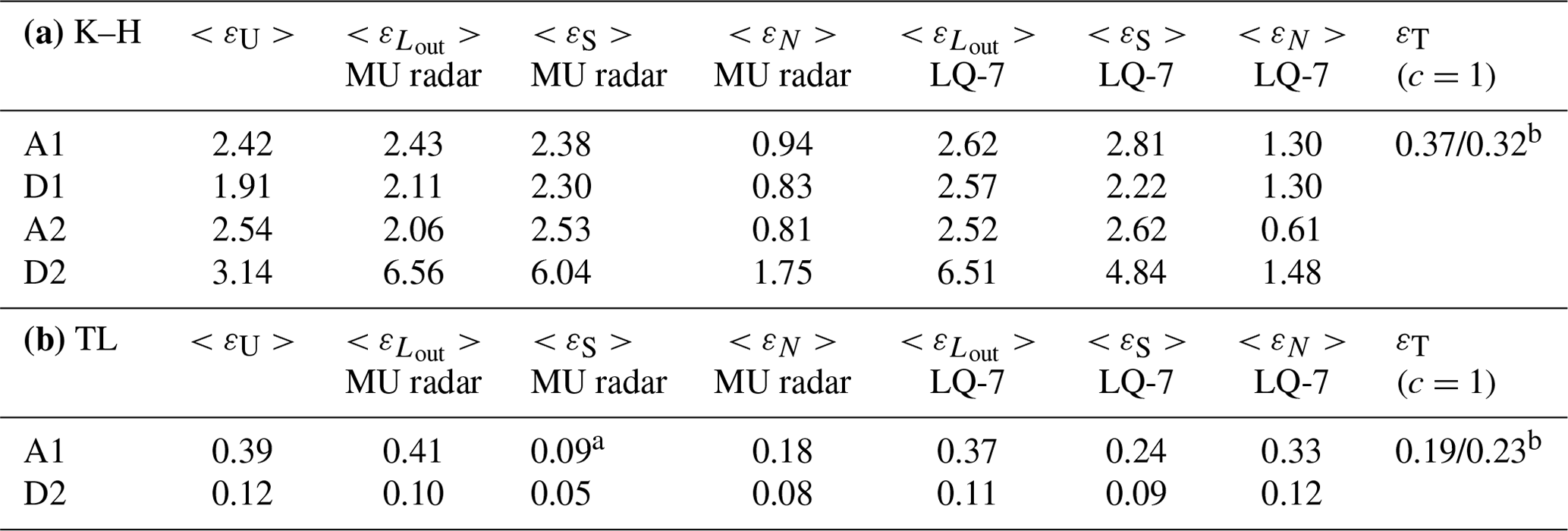
a This low value is due to a MU-radar-derived wind
shear about 2 times smaller than LQ-7- and balloon-derived wind shear. It is
doubtful and will affect LH and LC in Table 4.
b (sorted/rms).
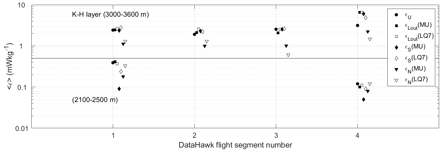
Figure 4Graphical representation of the averaged estimates of TKE dissipation rates (mW kg−1) (1 mW kg m2 s−3) shown in Table 3 for the K–H layer (3000–3600 m) sampled four times (top) and the layer between 2100 and 2500 m sampled twice during A1 (segment no. 1) and D2 (segment no. 4) (bottom). The horizontal black line at 0.5 mW kg−1 separates the two cases, and each radar-derived value has been successively shifted to the right by 0.025 with respect to segment numbers for clarity.
4.1.2 Comparison between DataHawk-derived ε and εT
The altitude and depth of the turbulent layers identified by the Thorpe method from V6 and εT (Eq. 6) with c=1 are shown by the dots and the solid vertical segments, respectively, in grey in Fig. 2a and in magenta in Fig. 3d. In Fig. 3d, values (Eq. 7) with , and are also shown for the K–H layer at 3.33 km and the turbulent layer at 2.37 km discussed in Sect. 4.2. and for the K–H layer are and s−2, respectively, i.e., s−2 on average. Because LT=130 m in the K–H layer, we obtain εT≈0.35 mW kg−1, which is about 7 times lower than DataHawk-derived ε (2.4 mW kg−1) (Table 3a). The hypothesis that V6 passed through the K–H layer in a region where ε was much lower is not consistent with the low variability (stationarity) of the dissipation rates estimated from DataHawk and radar data for more than 40 min (see Table 3a and Fig. 4). We therefore assume that εT must be ≈2.4 mW kg−1. To achieve this condition with Eq. (6), we must have c=2.6.
On the other hand, estimating (Eq. 7) requires the retrieval of S, but there is no prescribed method to compute the vertical shear of horizontal wind from balloon data in the Thorpe layers. Here, we estimated S from the difference of the wind vectors at the extremities of the Thorpe layer and from a linear interpolation of the zonal and meridional wind components in the Thorpe layer. We found S=0.013 and 0.010 s−1, respectively, i.e., 0.0115 s−1 on average, so that Ri≈0.055. This value is close to the mean value (〈Ri〉=0.09) obtained at a vertical resolution of 20 m (Fig. 2b). The relevance of εT≈0.35 mW kg−1 obtained with c=1 from Eq. (6) can be tested from Eq. (8) with using and . We get Ri=0.15 and Ri=0.30, respectively. These values are significantly larger than 0.055. For S=0.0115 s−1 and , we get mW kg−1, i.e., about 11 times larger than DataHawk-derived ε. We must have to be consistent with the DataHawk-derived ε value. and (and found in Appendix B) reasonably meet the necessary correction, giving credence to the validity of Eq. (7). As a corollary, for Ri=0.055, we would get , i.e., the required value of c for Eq. (6) to be valid. The various estimates of for the Thorpe layer are shown in Fig. 3d. Although based on a fragile hypothesis (ε from Thorpe analysis of the radiosonde data is equal to DataHawk-derived ε), Eq. (7) appears to be more adapted than the standard model (Eq. 6). It also has the major advantage over Eq. (6) that c′ is a true constant, at least when Ri<0.25, although its value remains to be defined more precisely.
4.1.3 Comparison of turbulence scales estimated from radar data
Table 4a shows the Hunt, Corrsin, buoyancy and Ozmidov length scales for the K–H layer calculated from WPR-LQ-7-derived and MU-radar-derived ε, σ and S during A1, D1, A2 and D2. N2 is computed from balloon data at the radar resolutions (100 m for the WPR-LQ-7 and 150 m for the MU radar). Once the scales are calculated, they are averaged over the altitude range 3000–3600 m of the K–H layer to compare them with the Thorpe length. All the radar-derived scales reveal the same behaviors between the segments A1, D1, A2, and D2 and do not show substantial differences between the radars, reinforcing the reliability of numerical results and their interpretations. Only the average values for A1, D1, A2 and D2 are discussed. We get 〈LH〉=46 m, 〈LC〉=38 m, 〈LB〉=105 m and 〈LO〉=131 m. 〈LH〉 and 〈LC〉 are substantially smaller than 〈LB〉 or 〈LO〉, indicating the latter should not be the scales to consider, as expected from the analysis of Sect. 4.1.1. Depending on the flight segment (A1, D1, A2, D2), was found between 0.65 and 1.56 and ∼ 1 on average. In contrast, we get 0.23–0.37. It is smaller than but close to and the value obtained in Appendix B () and the needed value of 0.31. We obtain and . Both radar estimates are significantly larger than Ri estimated from balloon data with the Thorpe analysis but are close to 〈Ri〉=0.33 estimated from balloon data at the vertical resolution of 100 m (Fig. 2b). The quantitative disagreements result mainly from comparisons between estimates made with different techniques (radar and in situ) and resolutions. Nevertheless, it is interesting to note that these comparisons tend to corroborate the conclusions obtained from in situ measurements alone (Sect. 4.1.2).
Table 4Mean values of Hunt, Corrsin, buoyancy and Ozmidov length scales for the K–H layer (a) and for the turbulent layer (TL) between 2100 and 2500 m (b).
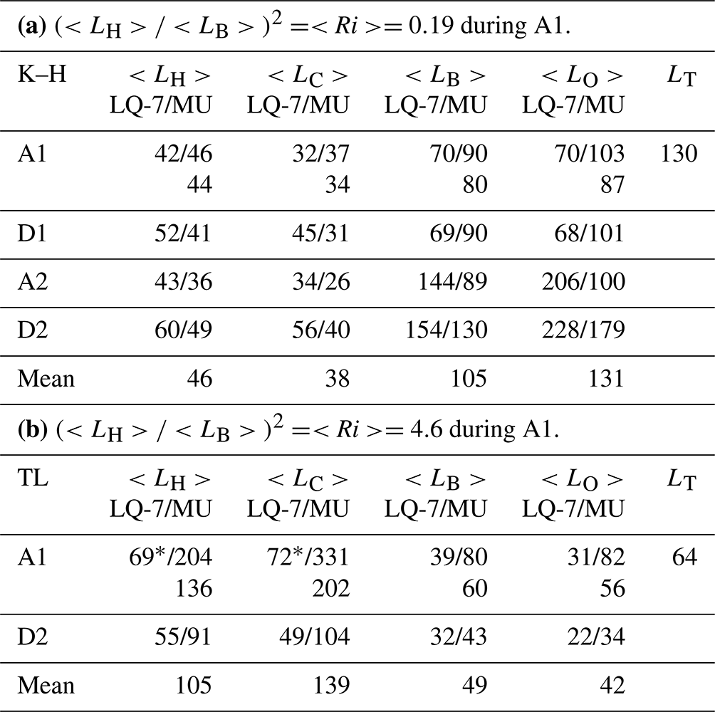
* Doubtful (see Table 3).
4.2 The turbulent layer between 2100 and 2500 m
Using the same methods as for the K–H layer, we obtain 〈Ri〉=0.75 (14.5) at a vertical resolution of 20 (100) m from V6 data (Fig. 2b), Ri≈2.0 from Thorpe analysis of V6 in the altitude range [2100–2500 m] (not shown) and 〈Ri〉=4.6 from N2 calculated at a vertical resolution of 100 m from V6 data and S calculated from WPR-LQ-7 data during A1 and D2 (Table 4b). Therefore, the Richardson number strongly varies according to the method and data used, but all the estimates are consistent with a Ri value significantly larger than for the K–H layer and likely larger than 1 (Sect. 4.1). Therefore, the weakly stratified condition (Ri<0.25) for which the alternative Eqs. (4) and (7) are valid is likely not verified for this layer. DataHawk-derived ε is about 1 order of magnitude lower than for the K–H layer: ∼ 0.2 mW kg−1 on average (Table 3b). The mean value is less reliable during D2. Many values of DataHawk-derived ε are missing because the algorithm did not detect a subrange in the velocity spectra (see L18). Figure 2a, Table 3b and Fig. 4 show that and εN and their mean values derived from both radars and εT are close to each other (within a factor of less than ∼ 2) and are very consistent with DataHawk-derived ε. All the radar and DataHawk estimates together show a temporal decrease by a factor of 3 to 4 in the 40 min between A1 and D2 (Fig. 4), giving credence that the agreements between the various estimates during A1 and D2 are not fortuitous. The temporal decrease of ε is consistent with a decaying turbulence when Ri>1. 〈εS〉 shows the largest discrepancies with DataHawk-derived ε, perhaps because the model is not valid for large Ri values. 〈LH〉 and 〈LC〉 (136 m and 202 m, respectively) exceed 〈LB〉=60 m and 〈LO〉=56 m, which are close to LT (64 m) (Table 4b). Therefore, 〈LH〉 and 〈LC〉 should not be the turbulence scales to consider. From the Thorpe analysis, s−2 and S≈0.0026 s−1 (Ri≈2). From Eq. (6) with c=1, εT≈0.2 mW kg−1 (Table 3b), i.e., very close to the mean value of DataHawk-derived ε or only 2 times lower than the value during A1. It is consistent with the fact that LT can be assimilated to LO. From Eq. (7) with Ri=2, and , we obtain and 0.004 mW kg−1, respectively, which is much less than 0.2 mW kg−1. The various estimates of are shown in Fig. 3d. As expected fails because it is expected to be valid for Ri<0.25 only.
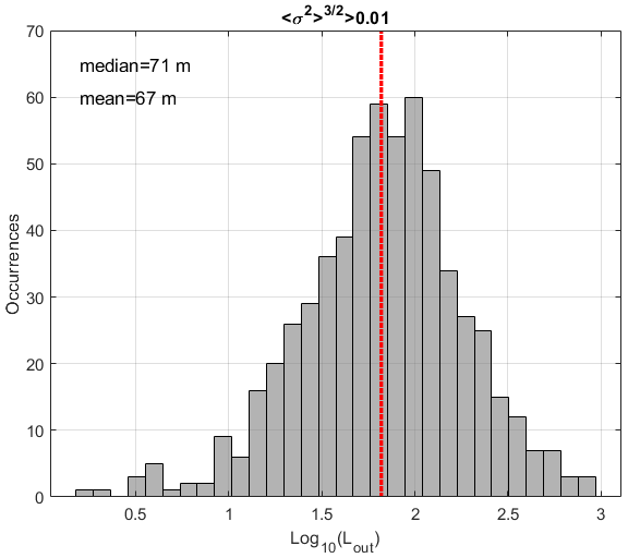
5.1 Justification of the application of Lout=70 m in Eq. (2)
Figure 5 shows the histogram of log 10(L), where for as in L18 obtained from the WPR-LQ-7 from data collected during 36 flights (corresponding to 90 profiles). The peak of the distribution has a mean (median) value of 67 m (71 m). These values are almost identical to those obtained from comparisons with MU radar, i.e., 75 m (61 m) (Fig. 7a of L18). This result seems to indicate that the empirical expression with Lout=70 m is not specific to the MU radar but at least to any radar with similar resolution volume (Table 2). However, the acquisition time of the MU radar and WPR-LQ-7 data differs by a factor of ∼ 2.5 (Table 2). It is likely fortunate that the statistical values of (and thus σ) coincide so well.
5.2 Statistical evaluation of the models from comparisons with εU
Figure 6a, b and c show the scatter plots of log 10(εU) vs , log 10(εS) and log 10(εN) with Lout=70 m, the shear estimated from WPR-LQ-7 data and N from DataHawk data at a height resolution of 100 m. Figure 6d and e show the results assuming a constant shear (〈S〉=7.7 m s−1 km−1) and a constant N ( s−2). Of course, Fig. 6d and e differ only in the constant .
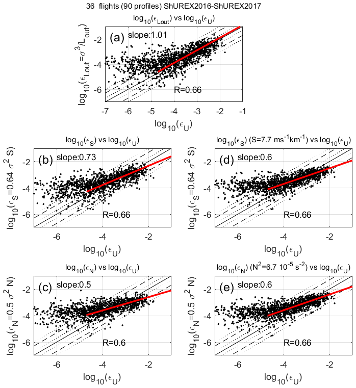
Figure 6Scatter plots of log 10(εU) vs (a) , (b) log 10(εS), (c) log 10(εN), (d) log 10(εS) with constant S and (e) log 10(εN) with constant N. The red lines are the result of a line regression (whose slope value is indicated in the panel) for m2 s−3, and R is the correlation coefficient.
The correlation coefficients are fortuitously ∼ 0.66 for all the cases except for εN for which the correlation is ∼ 0.60 only. This is an additional clue of the inadequacy of εN. The red lines show the results of linear regressions after rejecting dissipation rate values smaller than m2 s−3 as in L18, even though the quantitative threshold has no reason to be the same since the comparison methods differ. The slope of the regression line between and log 10(εU) is ∼ 1.0 (Fig. 6a), confirming the statistical σ3 dependence of ε when no discrimination is made on the conditions under which turbulence occurs. The regression slope obtained with log 10(εN) or log 10(εS) for S or N equal to a constant (Fig. 6d, e) is 0.60, i.e., close to , as expected because the two models vary as σ2. However, the regression slope between log 10(εU) and log 10(εN) with measured N (Fig. 6c) is significantly lower than 0.66 (0.50), and the regression slope between log 10(εU) and log 10(εS) with measured S (Fig. 6b) is significantly larger than 0.66 (0.73). The regression slope between log 10(εU) and log 10(εN) using MU radar data was 0.55 (L18), i.e., virtually identical to the present case (Fig. 6c). All the regression slopes depend on the quantitative threshold on ε, and, in Fig. 6a, it varies from ∼ 0.9 to ∼ 1.1 for different thresholds, excluding small values. However, all other slope estimates vary in concert, so that the observed trends remain valid for a different threshold.
- 1.
A regression slope between log 10(εU) and log 10(εS) that is closer to 1 than the slope between log 10(εU) and log 10(εN) indicates that εS provides estimates more consistent with than εN. Figure 7a and b show a comparison between the radar models, i.e., vs log 10(εN) and vs log 10(εS), respectively, for m2 s−3. The red lines are the results for constant N and constant S. The blue lines show the results of a linear regression. The blue and red lines obviously coincide (slope =0.60) for εN. A slope of 0.77 is obtained with εS, indicating a greater equivalence between and εS, as expected from Fig. 6b. Consequently, our results suggest that εS is more relevant than εN and should be used instead of εN for operational use if the empirical model is not chosen.
- 2.
We checked that generating a normal random distribution of N or S with a mean and standard deviation similar to the observed distributions produced a regression slope close to , similar to Fig. 6d and e. Therefore, the observed slopes with measured S and N (Fig. 6b, c) must reveal a statistical dependence of σ with and S, respectively. The equivalence between and εS described in Sect. 4 for the K–H layer implies that σ is simply proportional to S (σ=0.64 LoutS) if Lout is constant. There is a canonical value of Lout (∼70 m), but since Lout is not constant and is unknown (and can vary by 2 orders of magnitude at least; Fig. 5), the correlation between σ and S can only be established for a fixed value of Lout (and for any other variable on which σ depends). Figure 8 shows the same information as Fig. 7 but after dividing by σ2 to remove the self-correlation between the variables and to show the relationship between and log 10(0.5N) (Fig. 8a) and between and log 10(0.64S) (Fig. 8b). The two scatter plots show negative and positive correlation coefficients (−0.36 and 0.12, respectively). The correlations are weak but significant according to the P value. If no threshold on εU is applied, the correlation coefficients are −0.26 and +0.22. This suggests that σ increases to some extent as S increases and N decreases. It is quite intuitive, but, to our knowledge, this is the first study to suggest and highlight this. The results may reveal a Richardson number dependence. Figure 9a shows scatter plots of σ vs , where Ri100 (S100) now explicitly refers to the Richardson number (shear) calculated at the vertical resolution of 100 m. The red (black) dots show the results without and with a threshold on S100 (S100>5 m s−1 km−1), respectively. The (negative) correlation coefficient is slightly stronger with the threshold (−0.34 instead of −0.21). The high values of Ri100 are mainly associated with a weak shear (S100<5 m s−1 km−1) and with the largest variability in σ (Fig. 9a). However, this property may not be significant because the uncertainty on Ri increases as the shear tends to zero. Therefore, we focus on the scatter plot obtained with the threshold on the shear (black dots). It seems to show a linear dependence between log 10(σ) and , at least down to , i.e., for Ri100<0.4. Attempts of linear regression analysis do not confirm the linear trend, likely due to the strong dispersion and weak correlation. However, the time series obtained from the concatenation of all the profiles of and log 10(σ) after removing their mean values reveal a more obvious dependence between the two variables (Fig. 9b). The curves reveal similar variations and dynamics, especially for records [0−200], compatible with σ2 inversely proportional to Ri100, at least to a first approximation. For , i.e., for low values of Ri100(<0.4), log 10(σ) appears to have very little dependence on . If meaningful, it would be consistent with the fact that N does not play a significant role for low Ri values, as suggested by the εS model.
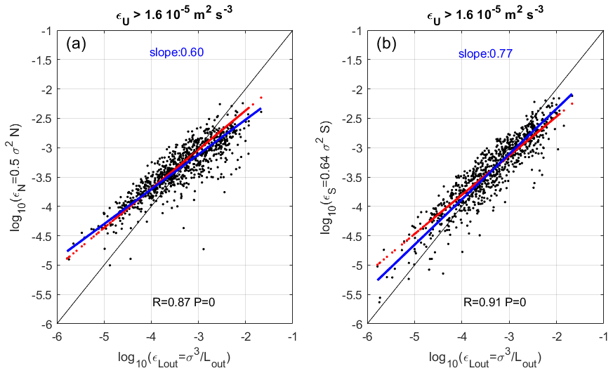
Figure 7Scatter plots of (a) vs log 10(εN) and (b) vs log 10(εS) for m2 s−3. The red lines show the results for constant N (a) and constant S (b). The blue lines show the results of a linear regression (whose slope value is indicated in the panel).
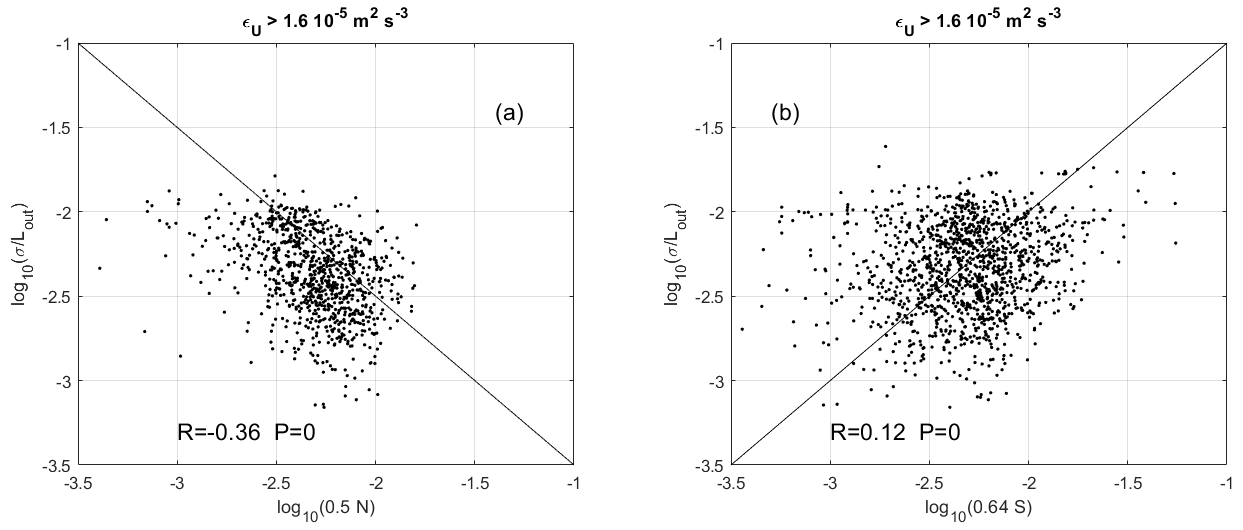
Figure 8Scatter plots of (a) log 10(0.5N) vs and (b) log 10(0.64S) vs for m2 s−3. R is the correlation coefficient, and P is the result of the P test.
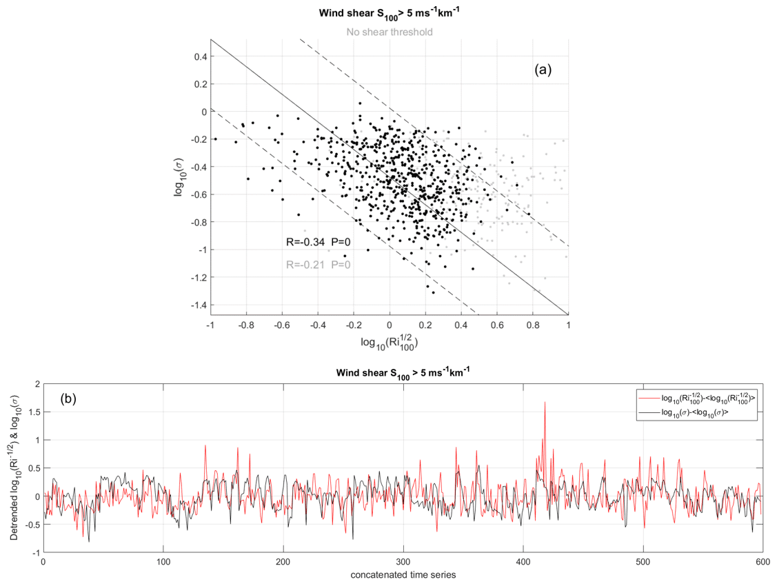
Figure 9(a) Scatter plots of vs log 10(σ) for m2 s−3 without the threshold on the shear (grey) and for S100>5 m s−1 km−1. (b) The corresponding time series of (grey) and log 10(σ) (black) after subtracting their mean.
Figure 10 shows the scatter plots of , and vs log 10(Ri100) applying two thresholds on εU: m2 s−3 in Fig. 10a, b and c and m2 s−3 in Fig. 10d, e and f. The latter is introduced to analyze the dependence of the results on the levels of considered dissipation rates. The red and blue curves show the values averaged in bandwidths of 0.3 from . For m2 s−3, the mean curves of and do not reveal a significant dependence on log 10(Ri100), at least up to log 10(Ri100)∼1, and are almost identical and close to 0 (Fig. 10a, c). Therefore, the applicability of the two models does not seem to depend significantly on the Richardson number on average. For m2 s−3, the curves produced by two models remain close and almost unchanged for log 10(Ri100)<0 (Fig. 10d, f). However, the mean values of now tend to decreases as log 10(Ri100) increases. Therefore, when log 10(Ri100)>0, εS tends to underestimate εU when εU exceeds ∼ m2 s−3 and inversely when m2 s−3. The fact that we experimentally observe that εS is not appropriate for large values of Ri100 is consistent with the expected domain of applicability of the model, even if it is not clear why it is in this way. For log 10(Ri100)<0, is less than 0 and decreases as log 10(Ri100) decreases for both thresholds (Fig. 10b, e). This experimental observation is a confirmation of the inadequacy of εN when the Richardson number is low. The results with are difficult to interpret when log 10(Ri100)>0. The model is consistent with εS when m2 s−3 (Fig. 10c) and seems to be more consistent with εN than with εS when m2 s−3 (Fig. 10e, f). It may be vain to interpret the properties of this model, since it is only an empirical model for which Lout=70 m only represents a canonical value of a function of multiple variables, including the shear and N.
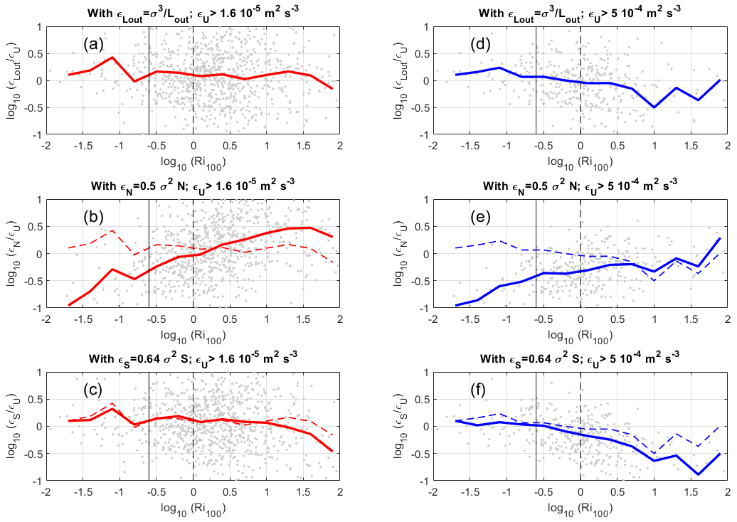
Figure 10Scatter plots of log 10(Ri100) vs (a, d) , (b, e) and (c, f) for m2 s−3 and m2 s−3, respectively.
The objective of this work was to test the suitability of TKE dissipation rate models based on Doppler radar spectral width measurements from comparisons with in situ estimates (εU) derived from high-resolution Pitot tube measurements aboard DataHawk UAVs. We showed the following:
- 1.
The models applied to the 46.5 MHz MU VHF radar by L18 produce statistically identical results on the 1.357 GHz WPR-LQ-7.
- a.
The empirical model with Lout∼70 m (as for the MU radar) provides the best statistical agreement with εU, at least for m2 s−3 (Table 2). If Lout really depends on the size of energy containing eddies, it is then independent of radar parameters (assuming σ2 is a true indication of 〈w′2〉 in both radars).
- b.
The model εN predicting a σ2N law for stably stratified conditions fails to reproduce εU. The biases are nearly quantitatively identical to those obtained with the MU radar: εN tends to overestimate when m2 s−3 and to underestimate when m2 s−3.
- a.
- 2.
Applying εN to both radars to a turbulent layer attributed to a K–H instability with Ri<0.25 strongly underestimates εU in the core of the layer when N2 is minimum. On the other hand, in agreement with the statistical results, εN provided values consistent with the other estimates in a turbulent layer, likely associated with larger Ri (≳1). These two observations are rather consistent with the domain of validity of εN according to the theoretical derivations (Eq. 5), leading to the newly introduced expression of εS expected to be valid for weakly stratified or strongly sheared conditions (e.g., Basu et al., 2021).
- 3.
The application of εS to the K–H layer (Ri<0.25) using both radars leads to a good agreement with εU. Its application to the turbulent layer associated with larger Ri slightly underestimates εU, again in accordance with Eq. (5).
- 4.
The statistical comparisons between εS and εU using all data show much better agreement than between εN and εU, although a bias of the same nature as that observed with εN is also noted but to a lesser degree. Empirical remains the most consistent model compared with εU. Lout∼70 m is likely a canonical value that results from all the hidden contributions of the various parameters that a most general (and unknown) model should include.
- 5.
The equivalence between εS and εU for the K–H layer associated with a low Ri necessarily implies that σ is proportional to S: σ∼0.64 LoutS. For all the layers with the same value of Lout, then σ linearly depends on S. This is a necessary condition if agreement is observed with two models that predict a σ3 and a σ2 dependence. For a wide distribution of log 10(Lout) as in Fig. 5, which includes values for all Ri, this linear dependence should be strongly “blurred” because Lout is variable, and Ri is not necessarily low. Moreover, an additional source of dispersion is that the wind shear calculated at the radar resolution S100 and at a time resolution of 10–30 min is not necessarily the most effective shear to be considered because S is a scale-dependent parameter (in the same way as Ri). As a result, a very weak, but yet significant, correlation between σ and S100 was found (Fig. 8). This weak correlation is responsible for the better agreement obtained with εS than with εN. However, because the results are based on a limited amount of data and because some degree of coincidence cannot be ruled out, further studies are necessary to analyze the dependence between σ and S100, in particular under more suitable conditions (i.e., low Ri).
- 6.
Reciprocally, σ has a statistical degree of dependence on , as revealed by the poorer statistical agreement between εN and εU, leading to a regression slope of less than (0.50, almost identical to 0.55 obtained from MU radar data by L18) (Fig. 6).
- 7.
The combination of points (5) and (6) leads to the conclusion that, to some extent, σ depends on , at least for Ri100≳0.4 (Fig. 9). This dependence does not seem to be valid for lower Ri100 (Fig. 8a), in accordance with the fact that N should not affect turbulence when the Richardson number is low (Eq. 4).
- 8.
The analysis of the three models, , εN and εS, with εU vs Ri100 (Fig. 10) confirms the good agreement between (, εU) and between (εS, εU) and the inadequacy of εN for Ri100≲1. The underestimation of εN increases as Ri100 decreases. The results for Ri100≳1 are more difficult to interpret and more puzzling, but εS and lead to comparable results and do not show substantial bias as a function of Ri100. In any case, all results involving large Ri (>1) must be taken with caution because the turbulence may be intermittent. In principle, the interpretation of the results should consider this.
- 9.
The classical model (Eq. 6) based on the equivalence between the Thorpe length LT and the Ozmidov length scale LO (c=1) fails to reproduce DataHawk-derived ε in the K–H layer for which Ri is expected to be less than 0.25. Although the disagreement can be due to several factors (e.g., an inappropriate choice of c, horizontal inhomogeneity), it can also be due to the fact the model involves the Ozmidov length scale defined for a turbulence affected by the stable stratification. In essence, LT cannot be related to LO anymore by a constant if the stratification effects can really be neglected for low Ri. Therefore, an alternative approach using the Corrsin length scale LC instead of LO was introduced, leading to (Eq. 7), compatible with studies showing a dependence of for Ri<0.25. Contrary to c, c′ is a true constant (with respect to Ri) for low Ri. It is worth noting that Eqs. (7) and (4) form a coherent pair of models independent of N for a weak stratification or strongly sheared flows. Using values of c′ deduced from the literature, provides estimates consistent with DataHawk- and radar-derived ε (expect εN) for the K–H layer. On the other hand, fails for a decaying turbulent layer (Ri>1) as the model is not expected to be valid for Ri>0.25. εT with c=1 shows a better agreement with DataHawk- and radar-derived ε (including εN), coherent with the fact that the stable stratification should affect the turbulence for large Ri. These results need to be confirmed by statistical studies.
The turbulent Froude number , where k refers to TKE for a simple and standard notation, is often used to characterize turbulent mixing (e.g., Ivey and Imberger, 1991). A strong and weak stratification is associated with Fr<1 and Fr>1, respectively. is called the inertial timescale and is a characteristic time of TKE dissipation. The corresponding timescales associated with the turbulence production by the wind shear and with the conversion into potential energy are S−1 and N−1, respectively. When the stratification is weak, i.e., when , then TL (dissipation time) and S−1 (production time) should be of the same order, i.e., the shear parameter STL=O(1), for stationary turbulence. Several studies (e.g., Mater and Venayagamoorthy, 2014, and references therein) reported a critical value for weakly stratified and stationary flows:
By dividing Eq. (A1) by 3.33 NTLc, we obtain
From the definition of Fr, Eq. (A2) reads
Assuming isotropy, , where 〈w′2〉 is the vertical velocity variance (assumed to be σ2 in the paper). We obtain
For (anisotropic) shear-generated turbulence, , so that
i.e., virtually Eq. (4) with CS=0.63. These expressions are valid for Fr>1, i.e., Ri<0.09, according to Eq. (A2).
For when (Eq. 28, Basu and Holtslag, 2021), we get
From Fig. (3) of Garanaik and Venayagamoorthy (2019), showing the turbulent Froude number Fr vs (or ) from DNS, we obtain, for weakly stratified conditions (Fr>1),
with α≈0.7. Note that this coefficient is deduced from their Fig. (3) using the linear trend shown by the authors. They did not explicitly refer to this value. By using the definitions (see Appendix A) and , Eq. (B1) can be re-written as
For Fr>1 or , STL≈3.33 (see Appendix 1 and Fig. 1 of Mater and Venayagamoorthy, 2014). Therefore, , so that
with . This value agrees well with the values reported in the main text.
In addition, by replacing Fr by its definition, Eq. (B2) can be re-written as , so that
Equation (B4) provides a way to relate the isotropic turbulent length scale Lk defined as the scale of the largest eddies weakly affected by the buoyancy and the shear to the Thorpe length: Lk∼1.5 LT. It also provides an expression of the master length scale LM defined as (e.g., Mellor and Yamada, 1982) with (Table 2, Basu and Holtslag, 2021). We obtain .
On the other hand, for strongly stratified conditions (Fr<1), we can write, from Fig. (3) of Garanaik and Venayagamoorthy (2019),
with according to the figure, or, purposely, . We obtain
so that
For , then, or
If , then . Equation (B5) demonstrates that the equivalence (at least the proportionality) between the buoyancy length scale and the Thorpe length is valid for strongly stratified conditions only (i.e., for conditions for which stability affects the vertical motions before being affected by the wind shear). For a weak stratification, the vertical TKE cannot be fully converted into potential energy because the parcels cannot move vertically over a length of LB (but LH only). Therefore, the basic stability does not intervene anymore in the variance of the vertical velocity fluctuations as in the case of a neutral stratification.
| α: | constant defined in Eq. (B1) |
| α′: | constant defined in Eq. (B5) |
| a.g.l.: | above ground level |
| a.s.l.: | above sea level |
| B: | buoyancy production/destruction term in Eq. (1) |
| β: | coefficient of proportionality between TKE and the variance 〈w′2〉 defined in Appendix B. |
| c: | constant in Eq. (6) |
| c′: | constant in Eq. (7) |
| : | constant in Eq. (7) for Schumann (1994) model |
| : | constant in Eq. (7) for Baumert and Peters (2000) model |
| CN: | constant in Eq. (3) |
| CS: | constant in Eq. (4) |
| : | pseudo-constant (depending on Rf) in Eq. (5a) |
| : | pseudo-constant (depending on Rf and G) in Eq. (5b) |
| DH: | DataHawk UAV |
| DNS: | direct numerical simulation |
| d′: | Thorpe displacement |
| ε: | TKE dissipation rate (general term) |
| : | ε estimated from radar data from Eq. (2) |
| εN: | ε estimated from radar data from Eq. (3) |
| εS: | ε estimated from radar data from Eq. (4) |
| : | ε estimated from radar data from Eq. (5a) |
| εT: | ε estimated from balloon data from Eq. (6) |
| : | ε estimated from balloon data from Eq. (7) |
| εU: | ε estimated from UAV data |
| F: | fraction of the inertial and buoyancy subrange contributions in Eq. (3) |
| FE: | full equilibrium |
| Fr: | Froude number |
| FFT: | fast Fourier transform |
| g: | gravitation acceleration |
| G: | growth factor |
| G0: | growth factor for Ri=0 |
| k: | an alternative notation for TKE (Appendix) |
| kB: | buoyancy wavenumber |
| kH: | Hunt wavenumber |
| KHI: | Kelvin–Helmholtz instability |
| L: | (Sect. 5.1) |
| LB: | buoyancy length scale |
| LC: | Corrsin length scale |
| LES: | large eddy simulation |
| LE: | Ellison length scale |
| LH: | Hunt length scale |
| LM: | master length scale defined in Appendix B |
| Lout: | an apparent outer scale of turbulence |
| LO: | Ozmidov length scale |
| LT: | Thorpe length |
| MU: | middle and upper atmosphere (radar) |
| N: | Brünt–Vaïsälä frequency |
| Ns: | Brünt–Vaïsälä frequency estimated from sorted θ profile |
| Nrms: | Brünt–Vaïsälä frequency estimated from the rms θ fluctuations |
| NINCOH: | number of incoherent integrations |
| P: | shear production term in Eq. (1) |
| Pr: | turbulent Prandtl number |
| R: | correlation coefficient |
| Rf: | flux Richardson number |
| Ri: | Richardson number |
| Ric: | critical Richardson number |
| Ris: | Richardson number at the FE condition |
| Ri100: | Richardson number estimated at a vertical resolution of 100 m |
| S: | vertical shear of horizontal wind |
| S100: | S estimated at a vertical resolution of 100 m |
| ShUREX: | Shigaraki UAV Radar EXperiment |
| σ2: | radar estimate of the variance 〈w′2〉 of the vertical wind fluctuations produced by turbulence |
| σobs: | half the measured Doppler spectral width |
| SNR: | signal-to-noise ratio |
| θ: | potential temperature |
| θ0: | half-power half width of the two-way radar beam |
| TKE: | turbulence kinetic energy |
| TL: | inertial timescale |
| τ: | radar pulse duration |
| UAV: | uncrewed aerial vehicle |
| UHF: | ultrahigh frequency |
| VHF: | very high frequency |
| WPR-LQ-7: | LQ-7 wind profiler |
| z: | altitude (a.g.l.) |
The WPR-LQ-7 data are available at http://www.rish.kyoto-u.ac.jp/radar-group/blr/shigaraki/data/ (RISH, 2023).
HL wrote the paper with the help of LK. LK, HL, HH, DL, AD, TM and MY carried out the observational campaign and participated in the collection and post-processing of the radar and UAV data and retrievals.
The contact author has declared that none of the authors has any competing interests.
Publisher’s note: Copernicus Publications remains neutral with regard to jurisdictional claims in published maps and institutional affiliations.
This research was partially supported by JSPS KAKENHI (grant no. JP15K13568) and the research grant for Mission Research on Sustainable Humanosphere from Research Institute for Sustainable Humanosphere (RISH), Kyoto University. Lakshmi Kantha acknowledges partial support from U.S. Office of Naval Research (ONR) MISO/BoB DRI (grant no. N00014-17-1-2716). Partial support to Dale Lawrence and Abhiram Doddi was provided by NSF Grant PDM 2128444 “New Pathways to Enhanced Turbulence and Mixing via Kelvin–Helmholtz Instability Tube and Knot Dynamics”.
This paper was edited by Wiebke Frey and reviewed by two anonymous referees.
Baumert, H. and Peters H.: Second-moment closures and length scales for weakly stratified turbulent shear flows, J. Geophys. Res., 105, 6453–6468, 2000.
Basu, S. and Holtslag, A. A. M.: Turbulent Prandtl number and characteristic length scales in stably stratified flows: steady-state analytical solutions, Environ. Fluid Mech., 21, 1273–1302, https://doi.org/10.1007/s10652-021-09820-7, 2021.
Basu, S. and Holtslag, A. A. M.: Revisiting and revising Tatarskii's formulation for the temperature structure parameter in atmospheric flows, Environ. Fluid Mech., 22, 1107–1119, https://doi.org/10.1007/s10652-022-09880-3, 2022.
Basu, S., He, P., and De Marco, A. W.: Parameterizing the energy dissipation rate in stably stratified flows, Bound.-Lay. Meteorol., 178, 167–184, https://doi.org/10.1007/s10546-020-00559-0, 2021.
Bertin, F., Barat, J., and Wilson, R.: Energy dissipation rates, eddy diffusivity, and the Prandtl number: An in situ experimental approach and its consequences on radar estimate of turbulent parameters, Radio Sci., 32, 791–804, https://doi.org/10.1029/96RS03691,1997.
Chen, Z., Tian, Y., and Lü, D.: Turbulence parameters in the troposphere-lower stratosphere observed by Beijing MST radar, Remote Sens.-Basel, 14, 947, https://doi.org/10.3390/rs14040947, 2022.
Clayson, C. A. and Kantha, L.: On turbulence and mixing in the free atmosphere inferred from high-resolution soundings, J. Atmos. Ocean. Tech., 25, 833–852, https://doi.org/10.1175/2007JTECHA992.1, 2008.
Cohn, S. A.: Radar measurements of turbulent eddy dissipation rate in the troposphere: a comparison of techniques, J. Atmos. Ocean. Tech., 12, 85–95, https://doi.org/10.1175/1520-0426(1995)012>0085:RMOTED>2.0.CO;2, 1995.
Dehghan, A. and Hocking, W. K.: Instrumental errors in spectral-width turbulence measurements by radars, J. Atmos. Sol.-Terr Phy., 73, 1052–1068, https://doi.org/10.1016/j.jastp.2010.11.011, 2011.
Dehghan, A., Hocking, W. K., and Srinivasan, R.: Comparisons between multiple in-situ aircraft turbulence measurements and radar in the troposphere, J. Atmos. Sol.-Terr Phy., 118, 64–77, https://doi.org/10.1016/j.jastp.2013.10.009, 2014.
Delage, D., Roca, R., Bertin, F., Delcourt, J., Crémieu, A., Masseboeuf, M., and Ney, R.: A consistency check of three radar methods for monitoring eddy diffusion and energy dissipation rates through the tropopause, Radio Sci., 32, 757–767, https://doi.org/10.1029/96RS03543, 1997.
Dole, J., Wilson, R., Dalaudier, F., and Sidi, C.: Energetics of small scale turbulence in the lower stratosphere from high resolution radar measurements, Ann. Geophys., 19, 945–952, https://doi.org/10.5194/angeo-19-945-2001, 2001.
Doviak, R. J. and Zrnić, D. S.: Doppler radar and weather observations, Academic Press, San Diego, ISBN 012221420X, 9780122214202, 1984.
Frisch, A. S. and Clifford, S. F.: A study of convection capped by a stable layer using Doppler radar and acoustic echo sounders, J. Atmos. Sci., 31, 1622–1628, https://doi.org/10.1175/1520-0469(1974)031<1622:ASOCCB>2.0.CO;2, 1974.
Fritts, D., Wang, L., Geller, M. A., Werne, J., and Balsley, B. B.: Numerical modeling of multiscale dynamics at a high Reynolds number: Instabilities, turbulence, and an assessment of Ozmidov and Thorpe scales, J. Atmos. Sci., 73, 555–577, https://doi.org/10.1175/JAS-D-14-0343.1, 2016.
Fukao, S., Yamanaka, M. D., Ao, N., Hocking, W. K., Sato, T., Yamamoto, M., Nakamura, T., Tsuda, T., and Kato, S.: Seasonal variability of vertical eddy diffusivity in the middle atmosphere. 1. Three-year observations by the middle and upper atmosphere radar, J. Geophys. Res.-Atmos., 99, 18973–18987, https://doi.org/10.1029/94JD00911, 1994.
Fukao, S., Luce, H., Mega, T., and Yamamoto, M.K., Extensive studies of large-amplitude Kelvin–Helmholtz billows in the lower atmosphere with VHF middle and upper atmosphere radar, Q. J. Roy. Meteorol. Soc., 137, 1019–1041, https://doi.org/10.1002/qj.807, 2011.
Garanaik, A. and Venayagamoorthy, S. K.: On the inference of the state of turbulence and mixing efficiency in stably stratified flows, J. Fluid Mech., 867, 323–333, https://doi.org/10.1017/jfm.2019.142, 2019.
Gerz, T., Schumann, U., and Elghobashi, S. E.: Direct numerical simulation of stratified homogeneous turbulent shear flows, J. Fluid Mech., 200, 563–594, https://doi.org/10.1017/S0022112089000765, 1989.
Hocking, W. K.: On the extraction of atmospheric turbulence parameters from radar backscatter Doppler spectra. I. Theory, J. Atmos. Terr. Phy., 45, 89–102, https://doi.org/10.1016/S0021-9169(83)80013-0, 1983.
Hocking, W. K.: Measurement of turbulent energy dissipation rates in the middle atmosphere by radar techniques: a review, Radio Sci., 20, 1403–1422, https://doi.org/10.1029/RS020i006p01403, 1985.
Hocking, W. K.: Observations and measurements of turbulence in the middle atmosphere with a VHF radar, J. Atmos. Terr. Phy., 48, 655–670, https://doi.org/10.1016/0021-9169(86)90015-2, 1986.
Hocking, W. K.: The dynamical parameters of turbulence theory as they apply to middle atmosphere studies, Earth Planets Space, 51, 525–541, https://doi.org/10.1186/BF03353213, 1999.
Hocking, W. K. and Hamza, A. M.: A quantitative measure of the degree of anisotropy of turbulence in terms of atmospheric parameters, with particular relevance to radar studies, J. Atmos. Sol-Terr. Phy., 59, 1011–1020, https://doi.org/10.1016/S1364-6826(96)00074-0, 1997.
Hocking, W. K., Röttger, J., Palmer, R. D., Sato, T., and Chilson P. B.: Atmospheric radar, Cambridge University Press, ISBN 9781107147461, 2016.
Hunt, J. C. R., Stretch, D. D., and Britter, R. E.: Length scales in stably stratified turbulent flows and their use in turbulence models, in: Stably stratified flow and dense gas dispersion, edited by: Puttock, J. S., Clarendon Press, Oxford, 285–321, 1988.
Imai, K., Nakagawa, T., and Hashiguchi, H.: Development of tropospheric wind profiler radar with Luneberg lens antenna (WPR LQ-7), Electric Wire & Cable, Energy, 64, 38–42, 2007.
Ivey, G. N. and Imberger, J.: On the nature of turbulence in a stratified fluid. Part I. The energetics of mixing, J. Phys. Oceanogr., 21, 650–659, https://doi.org/10.1175/1520-0485(1991)021<0650:OTNOTI>2.0.CO;2, 1991.
Jacoby-Koaly, S., Campistron, B., Bernard, S., Bénech, B., Ardhuin-Girard, F., Dessens, J., Dupont, E., and Carissimo, B.: Turbulent dissipation rate in the boundary layer via UHF wind profiler Doppler spectral width measurements, Bound.-Lay. Meterol., 103, 3061–389, https://doi.org/10.1023/A:1014985111855, 2002.
Jaiswal, A., Phanikumar, D. V., Bhattacharjee, S., and Naja, M.: Estimation of turbulence parameters using ARIES ST radar and GPS radiosonde measurements: First results from the Central Himalayan region, Radio Sci., 55, e2019RS006979, https://doi.org/10.1029/2019RS006979, 2020.
Kalapureddy, M. C. R., Kumar, K. K., Sivakumar, V., Ghosh, A. K., Jain, A. R., and Reddy, K. K.: Diurnal and seasonal variability of TKE dissipation rate in the ABL over a tropical station using UHF wind profiler, J. Atmos. Sol.-Terr. Phy., 69, 419–430, https://doi.org/10.1016/j.jastp.2006.10.016, 2007.
Kaltenbach, H.-J., Gerz, T., and Schumann, U.: Large-eddy simulation of homogeneous turbulence and diffusion in stably stratified shear flow, J. Fluid. Mech, 280, 1–40, https://doi.org/10.1017/S0022112094002831, 1994.
Kantha, L.: Turbulence dissipation rates in the free atmosphere from high-resolution radiosondes, in: Chap. 7: Turbulence:Theory, Types and Simulation, edited by: Marcuso, R. J., Nova Science Publ., 2010.
Kantha, L. and Hocking, W. K.: Dissipation rates of turbulence kinetic energy in the free atmosphere: MST radar and radiosondes, J. Atmos. Sol.-Terr. Phy., 73, 1043–1051, https://doi.org/10.1016/j.jastp.2010.11.024, 2011.
Kantha, L., Lawrence, D., Luce, H., Hashiguchi, H., Tsuda, T., Wilson, R., Mixa, T., and Yabuki, M.: Shigaraki UAV-Radar Experiment (ShUREX 2015): An overview of the campaign with some preliminary results, Progress in Earth and Planetary Science, 4, 19, https://doi.org/10.1186/s40645-017-0133-x, 2017.
Kohma, M., Sato, K., Tomikawa, Y., Nishimura, K., and Sato, T.: Estimate of turbulent energy dissipation rate from the VHF radar and radiosonde observations in the Antarctic, J. Geophys. Res.-Atmos., 124, 2976–2993, doi.org/10.1029/2018JD029521, 2019.
Kurosaki, S., Yamanaka, M. D., Hashiguchi, H., Sato, T., and Fukao, S.: Vertical eddy diffusivity in the lower and middle atmosphere: a climatology based on the MU radar observations during 1986-1992, J. Atmos. Sol.-Terr. Phy., 58, 727–734, https://doi.org/10.1016/0021-9169(95)00070-4, 1996.
Labitt, M.: Some basic relations concerning the radar measurements of air turbulence, MIT Lincoln Laboratory, ATC Working Paper NO 46WP-5001, 1979.
Li, Q., Rapp, M., Schrön, A., Schneider, A., and Stober, G.: Derivation of turbulent energy dissipation rate with the Middle Atmosphere Alomar Radar System (MAARSY) and radiosondes at Andøya, Norway, Ann. Geophys., 34, 1209–1229, https://doi.org/10.5194/angeo-34-1209-2016, 2016.
Luce, H., Kantha, L., Hashiguchi, H., Lawrence, D., Yabuki, M., Tsuda, T., and Mixa, T.: Comparisons between high-resolution profiles of squared refractive index gradient M2 measured by the Middle and Upper Atmosphere Radar and unmanned aerial vehicles (UAVs) during the Shigaraki UAV-Radar Experiment 2015 campaign, Ann. Geophys., 35, 423–441, https://doi.org/10.5194/angeo-35-423-2017, 2017.
Luce, H., Kantha, L., Hashiguchi, H., Lawrence, D., and Doddi A.: Turbulence kinetic energy dissipation rates estimated from concurrent UAV and MU radar measurements, Earth Planets Space, 70, 207, https://doi.org/10.1186/s40623-018-0979-1, 2018.
Mater, B. D. and Venayagamoorthy, S. K.: A unifying framework for parameterizing stably stratified shear-flow turbulence, Phys. Fluids, 26, 036601, https://doi.org/10.1063/1.4868142, 2014.
Mater, B. D., Schaad, S. M., and Venayagamoorthy, S. K.: Relevance of the Thorpe length scale in stably stratified turbulence, Phys. Fluids, 25, 076604, https://doi.org/10.1063/1.4813809, 2013.
McCaffrey, K., Bianco, L., and Wilczak, J. M.: Improved observations of turbulence dissipation rates from wind profiling radars, Atmos. Meas. Tech., 10, 2595–2611, https://doi.org/10.5194/amt-10-2595-2017, 2017.
Mellor, G. L. and Yamada, T.: Development of turbulence closure model for geophysical fluid problems, Rev. Geophys., 20, 851–875, https://doi.org/10.1029/RG020i004p00851, 1982.
Nastrom, G. D.: Doppler radar spectral width broadening due to beamwidth and wind shear, Ann. Geophys., 15, 786–796, https://doi.org/10.1007/s00585-997-0786-7, 1997.
Naström, G. D. and Eaton, F. D.: Turbulence eddy dissipation rates from radar observations at 5–20 km at White Sands Missile Range, New Mexico, J. Geophys. Res.-Atmos., 102, 19495–19505, https://doi.org/10.1029/97JD01262, 1997.
Naström, G. D. and Eaton, F. D.: Seasonal variability of turbulence parameters at 2 to 21 km from MST radar measurements at Vandenberg Air Force Base, California, J. Geophys. Res., 110, D19110, https://doi.org/10.1029/2005JD005782, 2005.
RISH: Boundary Layer Radar (BLR)/Lower Troposphere Radar (LTR)/LQ7 Observation Data, RISH (Research Institute for Sustainable Humanosphere) [data set], Version 02.0212, http://www.rish.kyoto-u.ac.jp/radar-group/blr/shigaraki/data/ (last access: 26 July 2023), 2023.
Satheesan, K. and Krishna Murthy, B. V.: Turbulence parameters in the tropical troposphere and lower stratosphere, J. Geophys. Res., 107, 4002, https://doi.org/10.1029/2000JD000146, 2002.
Schumann, U.: Correlations in homogeneous stratified shear turbulence, Acta Mech., 4, 105–111, 1994.
Schumann, U. and Gerz, T.: Turbulent mixing in stably stratified shear flows, J. Appl. Meteorol., 34, 33–48, https://doi.org/10.1175/1520-0450-34.1.33, 1995.
Shaw, W. J. and LeMone, M. A.: Turbulence dissipation rate measured by 915 MHz wind profiling radars compared with in-situ tower and aircraft data, in: 12th Symposium on Meteorological Observations and Instrumentation, Am. Meteorol. Soc., California, 2003.
Singh, N., Joshi, R. R., Chun, H.-Y., Pant, G. B., Damle, S. H., and Vashishtha, R. D.: Seasonal, annual and inter-annual features of turbulence parameters over the tropical station Pune (18∘32′ N, 73∘51′ E) observed with UHF wind profiler, Ann. Geophys., 26, 3677–3692, https://doi.org/10.5194/angeo-26-3677-2008, 2008.
Smyth, W. D., Moum, J. M., and Caldwell, D. R.: The efficiency of mixing in turbulent patches: Inferences from direct simulations and microstructure observations, J. Phys. Oceanogr., 31, 1969–1992, https://doi.org/10.1175/1520-0485(2001)031<1969:TEOMIT>2.0.CO;2, 2001.
Stull, R. B.: An Introduction to Boundary Layer Meteorology, Kluwer Academic, 666 pp., https://doi.org/10.1007/978-94-009-3027-8, 1988.
Weinstock, J.: Energy dissipation rates of turbulence in the free stable atmosphere, J. Atmos. Sci., 38, 880–883, https://doi.org/10.1175/1520-0469(1981)038<0880:EDROTI>2.0.CO;2, 1981.
White, A. B., Lataitis, R. J., and Lawrence, R. S.: Space and time filtering of remotely sensed velocity turbulence, J. Atmos. Sci. Tech., 16, 1967–1972, https://doi.org/10.1175/1520-0426(1999)016<1967:SATFOR>2.0.CO;2, 1999.
Wijesekera, H. W. and Dillon, T. M.: Shannon entropy as an indicator of age for turbulent overturns in the oceanic thermocline, J. Geophys. Res., 102, 3279–3291, https://doi.org/10.1029/96JC03605, 1997.
Wilson, R., Dalaudier, F., and Bertin, F.: Estimation of the turbulent fraction in the free atmosphere from MST radar measurements, J. Atmos. Ocean. Tech., 22, 1326–1339, https://doi.org/10.1175/JTECH1783.1, 2005.
Wilson, R., Luce, H., Hashiguchi, H., Nishi, N., and Yabuki, M.: Energetics of persistent turbulent layers underneath mid-level clouds estimated from concurrent radar and radiosonde data, J. Atmos. Sol.-Terr. Phy., 118, 78–89, https://doi.org/10.1016/j.jastp.2014.01.005, 2014.
- Abstract
- Introduction
- The radar models of ε
- The WPR-LQ-7 and methods of comparisons with UAV data
- Two case studies
- Statistical analysis
- Conclusions
- Appendix A
- Appendix B
- Appendix C: List of symbols
- Data availability
- Author contributions
- Competing interests
- Disclaimer
- Financial support
- Review statement
- References