Long-term multi-source precipitation estimation with high resolution (RainGRS Clim)

This paper explores the possibility of using multi-source precipitation estimates for climatological applications. A data-processing algorithm (RainGRS Clim) has been developed to work on precipitation accumulations such as daily or monthly totals, which are significantly longer than operational accumulations (generally between 5 min and 1 h). The algorithm makes the most of additional opportunities, such as the possibility of complementing data with delayed data, access to high-quality data that are not operationally available, and the greater efficiency of the algorithms for data quality control and merging with longer accumulations. Verification of the developed algorithms was carried out using monthly accumulations through comparison with precipitation from manual rain gauges. As a result, monthly accumulations estimated by RainGRS Clim were found to be significantly more reliable than accumulations generated operationally. This improvement is particularly noticeable for the winter months, when precipitation estimation is much more difficult due to less reliable radar estimates.

1 Introduction

The estimation of precipitation on the ground surface with high spatial resolution is one of the most important issues in meteorology but, at the same time, one of the most complex because of the very high spatial and temporal variability in precipitation, especially in the case of intense events associated with convective phenomena. This makes its precise quantitative estimation very difficult and subject to many errors. None of the available techniques, i.e. rain gauge measurements, meteorological radar measurements or satellite estimates based on measurements in different electromagnetic radiation bands, provide satisfactory precision. Consequently, different methods are being developed to combine precipitation data obtained by these techniques, with the aim of exploiting the advantages of each technique while minimising its weaknesses (Ochoa-Rodriguez et al., 2019; Jurczyk et al., 2020b; Wetchayont et al., 2023).

The generation of such multi-source precipitation estimates is currently the standard procedure used for quantitative precipitation estimation (QPE). In operational (i.e. real-time) applications, the most common time step for estimating the precipitation field is the 1 h step, as it often follows the demand from hydrological rainfall–runoff models (Sokol et al., 2021). However, sub-hourly resolutions, such as 10 min resolution, are also increasingly used. Such data are becoming essential, in particular as input for nowcasting precipitation forecast models; for rainfall–runoff models that forecast flash floods, which are triggered by intense but short-lived and rapidly fluctuating precipitation (e.g. Chan et al., 2016; Neuper and Ehret, 2019); or for performing analyses of the occurrence of precipitation extremes (e.g. Bonaccorso et al., 2020; Lengfeld et al., 2020; Marra et al., 2022).

However, there is also growing demand among climatologists and agrometeorologists, for example, for longer precipitation totals – of the order of days, months or years or even entire multi-year periods – that still maintain high spatial resolution. This demand can in fact already be met, as radar observations of precipitation, providing the highest spatial resolution of all measurement techniques, have been performed routinely for several decades. So, long series of radar as well as multi-source precipitation estimates are already available. Weather radar networks cover a large part of the more densely populated areas of the globe, so increasingly radar data, when supplemented with other observations, are also applied in climatological studies to provide extensive information on the multi-year variability in the precipitation field with very high spatial resolution not available with other measurement techniques (Fabry et al., 2017; Saltikoff et al., 2019a). They are also used to study the climatology of intense convective phenomena, as the high spatial resolution is particularly important in such cases (Hamidi et al., 2017; Burcea et al., 2019; Voormansik et al., 2021; Hänsler and Weiler, 2022; Piscitelli et al., 2022).

Consequently, there is a need to produce reliable estimates of precipitation accumulation over longer time periods (daily, monthly, yearly or even longer) with data from databases containing operationally generated multi-source precipitation at higher temporal resolutions, e.g. as 10 min precipitation accumulations. It turns out that simply adding up, for example, 10 min estimates does not give satisfactory results because any quality control algorithm for precipitation observations becomes much more effective for longer accumulations of at least 1 h (Morbidelli et al., 2018; Villalobos-Herrera et al., 2022). In particular, any algorithm for the adjustment of radar to rain gauge data often works too randomly when shorter accumulations are used, and the cross-checking of different types of precipitation data is then also subject to much higher uncertainty.

Generating accumulations for longer time intervals therefore provides the possibility of carrying out so-called reanalyses, i.e. re-generating the corresponding precipitation accumulation. This brings the following potential benefits: (i) datasets can be supplemented with data that were missing from the operational estimation, e.g. due to delays in their arrival at the system; (ii) in addition, data from such measurement techniques that are available too late for operational applications or measured with a longer calculation step (e.g. daily, such as from manual rain gauges) can be used (Imhoff et al., 2021); and (iii) algorithms for performing quality control on radar precipitation data and then combining these data with data from other sources generally work much more effectively for longer accumulations (Wagner et al., 2012; Park et al., 2019).

Various initiatives are being undertaken to estimate precipitation data for climatological purposes with the high spatial resolution obtained from radar observations, including on a trans-national scale. One of the major initiatives in this area is the EURADCLIM (EUropean RADar CLIMatology) dataset, which is based on radar data obtained from the Operational Programme for the Exchange of Weather Radar Information (OPERA) – a EUMETNET (European Meteorological Network) initiative (Saltikoff et al., 2019b) – and rain gauge data obtained from the European Climate Assessment & Dataset (ECA&D) project. Both of these networks are pan-European and cover most of Europe. In the EURADCLIM programme, radar quality control adapted to longer precipitation accumulation intervals, such as 1 h and daily intervals, is performed (Overeem et al., 2023). Quality control is also performed on longer rain gauge accumulations within ECA&D (Klok and Klein Tank, 2009).

The concept of generating long-term precipitation estimation presented in this paper is based on using algorithms for quality control of the input data and combining them into multi-source estimates, which are applied operationally to 10 min data. However, new quality control methods and new data sources have also been included – something that was not possible during the operational generation of precipitation estimates.

Section 2 describes all input data, those available operationally as well as those used for reanalyses. Section 3 presents the algorithm for combining precipitation data into a multi-source precipitation field, used both operationally and for reanalyses, and Sect. 4 proposes a scheme for generating long-term estimates. Section 5 shows and discusses the results of the verification of the reanalyses of monthly totals in different seasons compared to operationally generated estimates, while Sect. 6 shows an example of the system performance. Finally, Sect. 7 provides conclusions.

2 Precipitation data

2.1 Precipitation measurement data available for the area of Poland

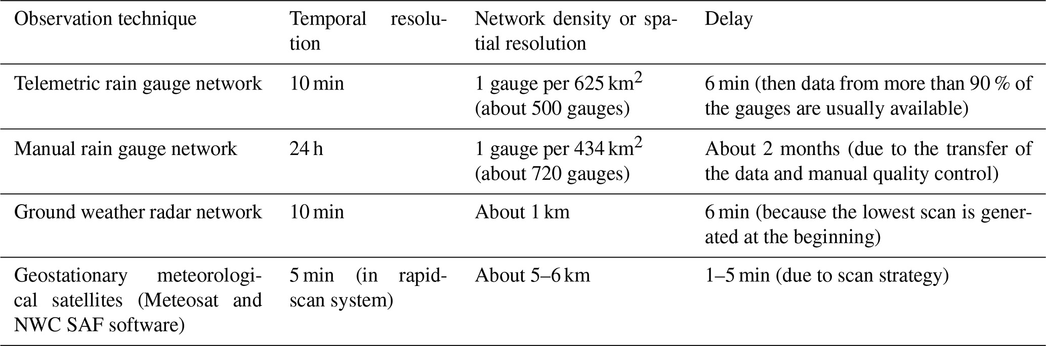
Table 1 summarises the general characteristics of the precipitation data available for the area of Poland: from in situ and remote sensing measurements, available both in real time and after a shorter or longer processing time, which can take up to 2 months (this is the case for quality control of the data from manual rain gauges).

Table 1 In situ precipitation measurement networks available for Poland.

This study uses precipitation data generated by the Institute of Meteorology and Water Management – National Research Institute (IMGW), which performs the function of the national meteorological and hydrological service in Poland (Szturc et al., 2018). All these data are quality-controlled by dedicated applications or systems.

2.2 Rain gauge data

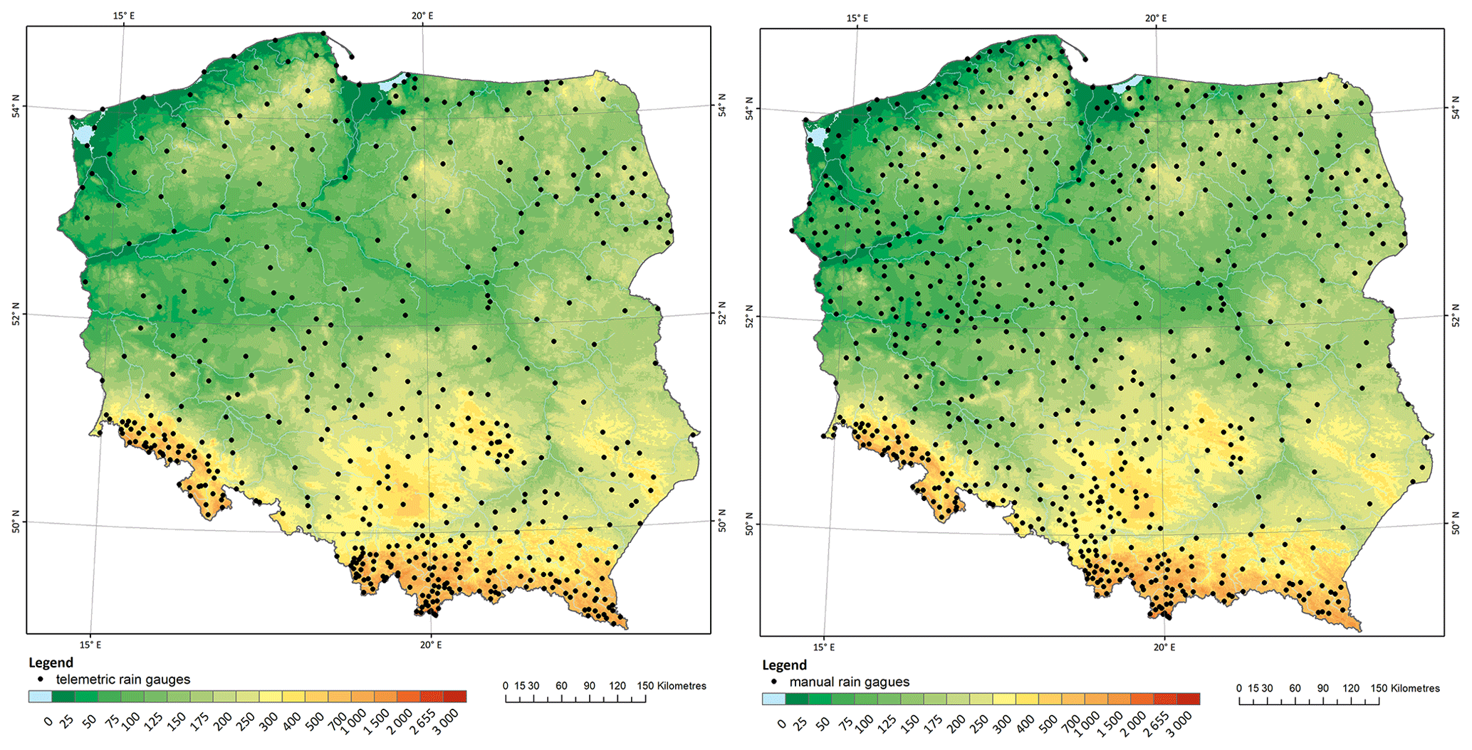
Figure 1 Rain gauge networks of IMGW. From left: telemetric and manual rain gauge networks.

The 10 min precipitation accumulations are provided operationally at IMGW by a network of telemetric rain gauges, most of which are tipping-bucket gauges – considered one of the less accurate of the various types of rain gauges (Hoffmann et al., 2016; Segovia-Cardozo et al., 2021) in addition to being subject to significant failure rates. For quality control of telemetric rain gauge data, the RainGaugeQC system is used at IMGW to perform error detection and corrections on 10 min data in real time (Ośródka et al., 2022).

One of the most important additional benefits of carrying out reanalyses, relative to the generation of a real-time precipitation field, is the possibility of exploiting the much more accurate measurements performed by manual rain gauges mostly once a day. The network of such rain gauges (Hellmann type) installed at IMGW is relatively dense and even denser than the network of telemetric rain gauges (Fig. 1 and Table 1). These are the most accurate of the in situ point measurements, but they are available with a very long delay of almost 2 months, mainly due to the human-made data quality control. In addition, measurements from manual rain gauges are subjected to quality control in the IMGW historical database, using standard algorithms based on procedures recommended by the World Meteorological Organization (WMO-No. 305, 1993, Chap. 6).

2.3 Weather radar data

The radar data used to generate the precipitation field estimates come from the Polish POLRAD weather radar network, operated by IMGW. It consists of eight Doppler radars manufactured by LEONARDO Germany (Fig. 2). They are currently being replaced by new models with dual-polarised radar beams, and two new radars are being installed. Three-dimensional raw data, so-called volumes (raw data), and two-dimensional products are generated by the Rainbow 5 system every 10 min (a shift to 5 min measurement frequency is currently underway), with 0.5 km spatial resolution and a range of 250 km. For further details on the POLRAD network, see Ośródka and Szturc (2022).

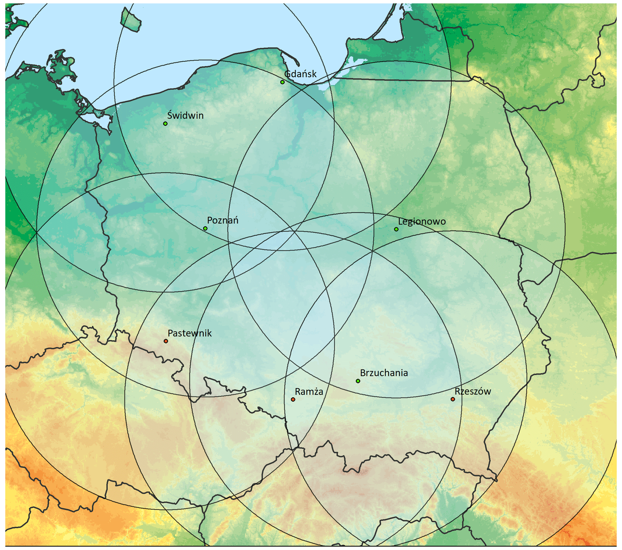
Figure 2 Computational domain of Poland (900 km × 800 km) with 250 km radar coverage of the weather radar network in Poland in 2022 (when the work presented here was carried out).

The RADVOL-QC system (Ośródka et al., 2014; Ośródka and Szturc, 2022) is used to quality-control radar data of the POLRAD network, which corrects the source 3D radar data and generates dynamic maps of the data quality index. Merging data from individual radars into radar composite maps is done by applying algorithms that take account of the spatial distribution of the quality index in the radar data, which is assessed dynamically for each time step (Jurczyk et al., 2020a).

2.4 Precipitation from meteorological satellites

Satellite precipitation is generated by an algorithm developed at IMGW based on products provided by the EUMETSAT NWC SAF programme (Tapiador et al., 2019). The algorithm working within the RainGRS system is based on several NWC SAF products that depict the spatial distribution of clouds and the intensity of precipitation, including convective precipitation. A detailed description of the algorithm was presented by Jurczyk et al. (2020b).

Quality control of satellite precipitation is also carried out by the RainGRS system, taking into account primarily which NWC SAF products are available at a given time. The quality of satellite precipitation, which is quantified by the quality index, is significantly lower at nighttime, when visible range-based products analysing the physical properties of hydrometeors are not available.

3 RainGRS system

3.1 Merging of precipitation data into a multi-source precipitation field

At IMGW, multi-source estimation of the precipitation field is carried out operationally by the RainGRS system. A detailed description of this system, which combines rain gauge, radar and satellite precipitation data summarised in Table 1, was presented by Jurczyk et al. (2020b). This combination algorithm takes into account the quality information of the individual input data, attributed to them when performing their quality control.

In operational work, the 10 min computational step of generating estimates of the precipitation field is enforced by the resolution of the radar data, which is the source of the most important high-resolution information on the spatial distribution of the precipitation field. When the radars of the POLRAD network are replaced (process is ongoing from 2022 to 2023), all included radars will operate with a 5 min time step. This will enable the temporal resolution of the multi-source precipitation estimates generated by RainGRS to be increased as well.

The algorithm for combining rainfall data from different sources is based on a conditional merging that attempts to enhance the strengths of the individual inputs and reduce the impact of their weaknesses. It is commonly assumed that radar data comprise the best representation of the spatial distribution of the precipitation field, while a network of rain gauges effectively reduces the bias of this estimation. Satellite rainfall, in contrast, plays a mainly complementary role in the absence of other data.

First, the rain gauge values are interpolated at radar pixel resolution, employing the ordinary kriging method to obtain an unbiased estimate of precipitation. The radar values at rain gauge locations and the same method of interpolation are used to get the interpolated radar field. Subsequently, the deviation between the measured and interpolated radar value (R−R_int) is computed and added to the rain gauge interpolated value at each pixel of the domain, according to the following formula:

$$\begin{array}{}\text{(1)}& R_{\mathrm{G}}=G_{\mathrm{int}}+\left(R-R_{\mathrm{int}}\right),\end{array}$$

where R_int is the radar precipitation interpolated from data at rain gauge locations. A satellite field S_G is obtained from an analogical formula.

It can be noted that the accuracy of the computed estimate depends on the distance to the nearest available rain gauge, and the radar precipitation field is preferable in the case of a long distance. Therefore, the resulting precipitation field R_G is recombined with the radar precipitation field, applying the weighted scheme, which includes the quality of individual precipitation fields, to obtain a combined GR field:

$$\begin{array}{}\text{(2)}& \mathrm{GR}={\displaystyle \frac{R_{\mathrm{G}}\cdot {\mathrm{QI}}_{\mathrm{G}}+R\cdot {\mathrm{QI}}_{\mathrm{R}}\cdot \left(\mathrm{1}-{\mathrm{QI}}_{\mathrm{G}}\right)}{{\mathrm{QI}}_{\mathrm{G}}+{\mathrm{QI}}_{\mathrm{R}}\cdot \left(\mathrm{1}-{\mathrm{QI}}_{\mathrm{G}}\right)}},\end{array}$$

where QI_G and QI_R are the quality indices for gauge and radar, respectively. The quality index, QI, is the dimensionless quantity ranging from 0 (for the poorest quality) to 1 (for the best data).

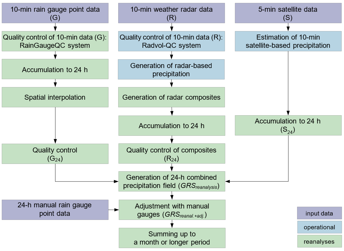
Figure 3 The algorithm for determining quality-controlled daily, monthly and other precipitation accumulations.

A combined gauge–satellite field GS is obtained analogically to the above procedure, where the satellite data S and relevant quality field QI_S are taken.

The final quantitative precipitation estimate (GRS) is a combination of gauge–radar and gauge–satellite fields computed by means of the following weighted formula:

$$\begin{array}{}\text{(3)}& \mathrm{GRS}={\displaystyle \frac{\mathrm{GR}\cdot {\mathrm{QI}}_{\mathrm{d}}+\mathrm{GS}\cdot (\mathrm{1}-{\mathrm{QI}}_d)\cdot {\mathrm{QI}}_{\mathrm{S}}}{{\mathrm{QI}}_d+{\mathrm{QI}}_{\mathrm{S}}\cdot (\mathrm{1}-{\mathrm{QI}}_d)}},\end{array}$$

where QI_d is a field of radar data quality as a function of the distance d to the nearest radar site.

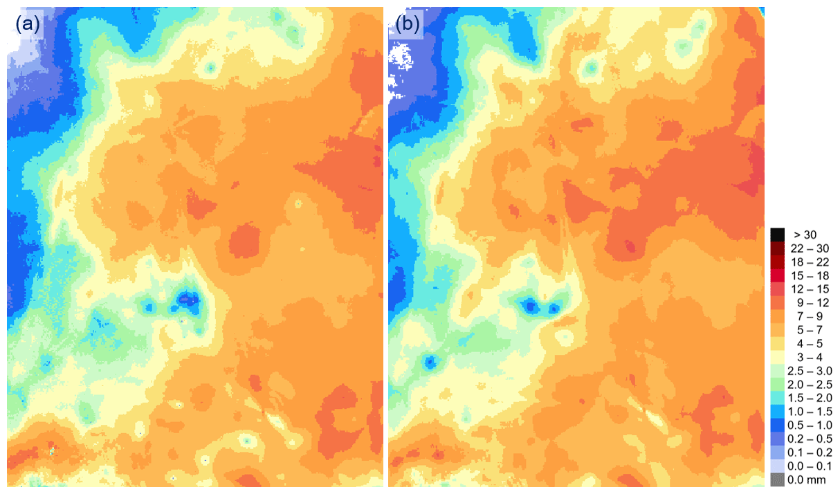
Figure 4 Fields of daily precipitation accumulations, before and after reanalysis: (a) GRS_real-time and (b) GRS_reanalysis. Fragment of Poland's computational domain (325 km × 425 km), 11 December 2022.

3.2 Generation of daily accumulations

The basic 10 min precipitation accumulations are aggregated into different time intervals (e.g. 1 h, several hours, daily, or longer accumulations) depending on current needs. Due to gaps in data that occur in operational work, sometimes these accumulations may not be complete. In order to ensure the completeness of the accumulations, the gaps are complemented by temporal interpolation of the data from time steps directly before and after the gap. Such averaging from neighbouring measurements is carried out if this interval is not too long, and in the opposite case, data are set to have no data value. For example, when generating hourly accumulation, at most two consecutive 10 min measurements are allowed to be missing, but no more than three terms may be missing in 1 h.

4 Generation of daily and monthly precipitation reanalyses (RainGRS Clim)

4.1 Climatological reanalyses versus operational estimates

Reanalysis of the precipitation fields is carried out using daily accumulations. This provides the following benefits in terms of the reliability of the generated estimates:

1. Complementation with data that were missing operationally due to their late arrival in the system. For reanalyses, a time regime is not as strict as in an operational work, so data that arrived too late can be included. In the operational RainGRS, more than 90 % of the rain gauge data generally arrive within 6 min, so the remaining data can be involved in reanalyses. When it comes to radar data, delays mainly affect data from foreign radars.

2. The use of measurement techniques that are available too late to be used operationally or that take measurements with a time step longer than 10 min as standard. In the proposed algorithm for performing reanalyses, in addition to using daily precipitation accumulations provided by those measurement techniques from which data are operationally available, data from manual rain gauges can also be used. These measurements are taken only once a day and are available after about 2 months – for this reason they are not used in the operational version of RainGRS, but due to their high reliability, these data are very important, even crucial.

3. Greater effectiveness of quality control and data merging algorithms when applied to accumulations longer than 10 min, e.g. daily. Longer precipitation accumulations are more consistent, as they are much less affected by temporal inconsistencies between different measurement techniques (this is especially the case with radar measurements, which in practice are instantaneous) and are moreover less sensitive to errors of a random nature, which become more averaged over a longer time interval. Thus, the algorithms for both quality control and multi-source combination perform more effectively.

At IMGW, combined daily accumulations have been generated since 2021 by the algorithm described in this paper. The resulting daily precipitation estimates can already be directly used to generate longer precipitation accumulations, e.g. monthly, seasonal, annual or even multi-year. In view of the above possibilities, which create new areas of application for multi-source precipitation fields, e.g. in climatology, the version of RainGRS that generates reanalyses of daily precipitation accumulation is referred to as RainGRS Clim.

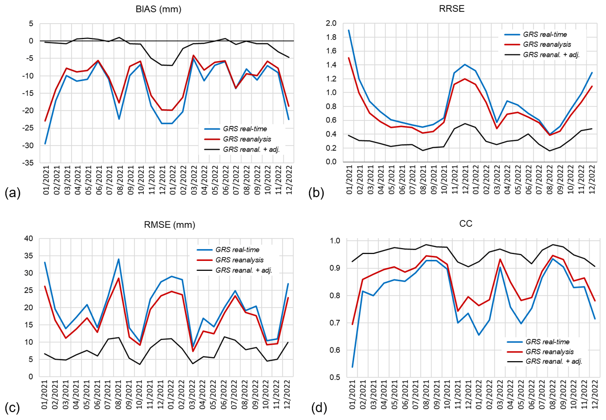
Figure 5 Values of monthly characteristics: (a) bias, (b) RRSE, (c) RMSE and (d) CC, for precipitation estimates GRS_real−time, GRS_reanalysis, and GRS${}_{\mathrm{reanal}.+\mathrm{adj}.}$ for consecutive months, using point data from manual rain gauges as reference. Data for 2021 and 2022.

4.2 Algorithm for the estimation of climatological multi-source precipitation fields

The algorithm presented in this section for calculating quality-controlled daily and monthly rainfall totals follows the following scheme (Fig. 3):

1. Daily totals are calculated from 10 min rain gauge data. In order to ensure the completeness of the 10 min data, missing rain gauge data are completed with spatially interpolated values from the data that are available. The ordinary kriging method is used to interpolate the data.

2. The daily point accumulations from the rain gauges are spatially interpolated to obtain precipitation fields.

3. A human expert check of the daily rain gauge fields is carried out, during which erroneous values from individual rain gauges are removed. This check on the daily values enables the detection of errors that were not detected in the 10 min accumulations with automatic quality control (QC) algorithms. The daily accumulations from the rain gauges are then spatially interpolated again (as in point 2).

4. Daily accumulations of radar and satellite precipitation fields are calculated, also supplemented with late data.

5. The daily radar precipitation fields are corrected by removing disturbances occurring at the locations of some radars, as this correction only works effectively on longer accumulations.

6. Estimates of daily accumulations GRS_reanalysis are calculated by the RainGRS system using the algorithm described in Sect. 3.1, which uses daily accumulations of individual precipitation fields as input data. This approach minimises errors associated with temporal inconsistencies in the data (Villalobos-Herrera et al., 2022).

7. An adjustment of daily accumulations calculated by the RainGRS to observations from manual rain gauges, which are considered to give the most reliable point estimates of rainfall, is performed. The adjustment factor is determined separately for each manual rain gauge location and then spatially interpolated using the inverse distance weighting method to distribute it spatially (Wang et al., 2020). This adjustment results in daily accumulations GRS${}_{\mathrm{reanal}.+\mathrm{adj}.}$ of multi-source rainfall fields after reanalysis and adjustment.

8. The long-term accumulations of the combined precipitation fields (e.g. monthly) can be calculated from the daily accumulations prepared in the above manner.

Figure 4 shows an example of daily rainfall accumulations obtained operationally and after reanalysis. The differences between the two fields are generally not large, but locally they can be quite significant – a fragment from the computational domain is selected to highlight them. Larger differences between them are apparent in cases where some rain gauge data have been removed as a result of manual QC (during which they were found to be clearly erroneous) and this was not recognised by operational control. It is likely that in the 10 min accumulations, the measurement errors were not noticeable enough to consider these values completely erroneous. The removal of each such value also affects the values in a certain vicinity of the rain gauge's location due to changes in the field of interpolated gauges, relevant QI field and consequently RainGRS field. In addition, some of the differences between the two fields are due to the varying performance of the data combination algorithm (Sect. 3.1) applied to daily accumulations when compared to 10 min ones.

5 Verification

5.1 Methodology of the verification

In order to verify any precipitation field estimate, a precipitation field reference that can be considered “ground truth” is needed. Lysimeters are regarded as one of the most accurate point precipitation measurement techniques, but Hellmann-type manual rain gauges have similar reliability (Hoffmann et al., 2016). IMGW does not have at its disposal a network of lysimeters; however, it does have a relatively dense network of manual Hellmann-type rain gauges. Therefore these were considered to provide the most accurate technique of point measurement of precipitation available in IMGW. Thus, the results obtained in the present study were verified on them.

Table 2 Values of quality metrics for merged daily precipitation fields: before reanalysis (GRS_real−time), after reanalysis (GRS_reanalysis), and after reanalysis and adjustment $\left({\mathrm{GRS}}_{\mathrm{reanal}.+\mathrm{adj}.}\right)$, using point data from manual rain gauges as reference. Months: (a) January 2022 and (b) August 2022.

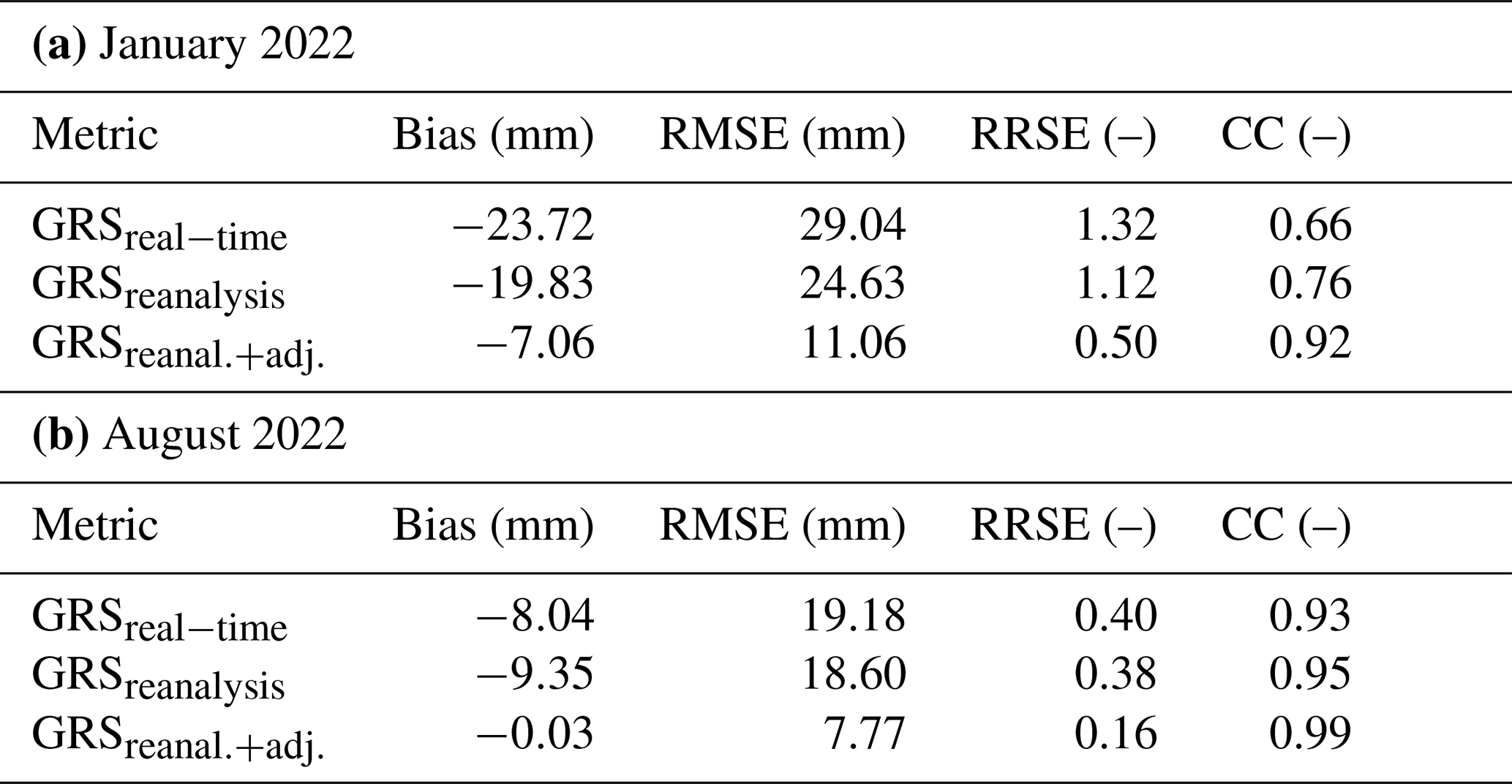
However, it should be borne in mind that the data from the manual rain gauges are not independent, as they have previously been used for adjustment of the RainGRS Clim data. Thus, the basic quantity verified in this section is not the final precipitation estimates produced after adjustment to the manual rain gauge data but the estimates after quality control and reanalysis, i.e. GRS_reanalysis. However, the verification of the final reanalyses ${\mathrm{GRS}}_{\mathrm{reanal}.+\mathrm{adj}.}$ also provides interesting information, though one should be careful especially with criteria directly related to the estimated values, such as bias or RMSE, rather than, for example, their correlation with the reference field.

The period from January 2021 to December 2022 was analysed. For each of these 24 months, the statistics of the monthly precipitation estimates – bias, RRSE, RMSE and CC – were calculated, taking the accumulations from the manual rain gauges as reference:

• statistical bias,

  $$\begin{array}{}\text{(4)}& \mathrm{bias}={\displaystyle \frac{\mathrm{1}}{n}}{\sum }_{i=\mathrm{1}}^n\left(F_i-O_i\right);\end{array}$$

• root mean square error,

  $$\begin{array}{}\text{(5)}& \mathrm{RMSE}=\sqrt{{\displaystyle \frac{\mathrm{1}}{n}}{\sum }_{i=\mathrm{1}}^n{\left(F_i-O_i\right)}^{\mathrm{2}}};\end{array}$$

• root relative square error,

  $$\begin{array}{}\text{(6)}& \mathrm{RRSE}={\displaystyle \frac{\sqrt{{\sum }_{i=\mathrm{1}}^n{\left(F_i-O_i\right)}^{\mathrm{2}}}}{\sqrt{{\sum }_{i=\mathrm{1}}^n{\left(O_i-\stackrel{\mathrm{‾}}{O}\right)}^{\mathrm{2}}}}};\end{array}$$

• Pearson correlation coefficient,

  $$\begin{array}{}\text{(7)}& \mathrm{CC}={\displaystyle \frac{{\sum }_{i=\mathrm{1}}^n\left(F_i-\stackrel{\mathrm{‾}}{F}\right)\left(O_i-\stackrel{\mathrm{‾}}{O}\right)}{\sqrt{{\sum }_{i=\mathrm{1}}^n{\left(O_i-\stackrel{\mathrm{‾}}{O}\right)}^{\mathrm{2}}{\sum }_{i=\mathrm{1}}^n{\left(F_i-\stackrel{\mathrm{‾}}{F}\right)}^{\mathrm{2}}}}}.\end{array}$$

In the above, F_i is the assessed value, O_i is the reference value (from manual rain gauges), i is the pixel number, n is the number of pixels, and $\stackrel{\mathrm{‾}}{F}$ and $\stackrel{\mathrm{‾}}{O}$ are the mean values of F_i and O_i.

5.2 Monthly statistics

Figure 5 shows how the values of the four statistics, bias, RRSE, RMSE and CC, change in the following months, i.e. depending on the seasonal precipitation characteristics.

The most evident phenomenon visible in the bias graph is large underestimation of monthly precipitation accumulations, especially in winter months (December–February), that can reach up to 20 mm (Fig. 5a), which in Poland means several dozen percent of monthly accumulations. This is a result of the fact that the precipitation measurements from both rain gauges and radars are underestimated in IMGW due to the use of specific types of measuring devices, as mentioned in Sect. 2.2 and 2.3. Additionally, in winter the reason for these errors is the difficulty in radar measurements that occurs during snowfall from lower clouds compared to in other seasons and causes most of this precipitation to become invisible to radar as a result of overshooting the precipitation by the radar beam.

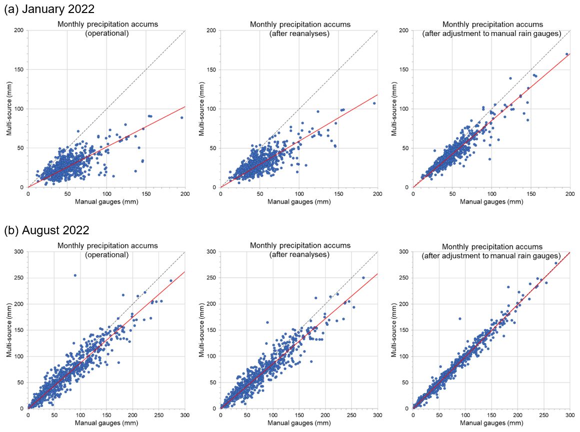
Figure 6 Plots of the dependence of monthly precipitation estimate values (from left: GRS_real−time, GRS_reanalysis and ${\mathrm{GRS}}_{\mathrm{reanal}.+\mathrm{adj}.}$) on values measured with manual rain gauges, along with trend lines. Months: (a) January 2022 and (b) August 2022. The abbreviation “accums” denotes accumulations.

Reanalysis and quality control applied to daily accumulations lead to a reduction in bias by a few millimetres per month, mainly in the winter months. This is mostly due to the clearly better performance of the algorithm for the combination of rain gauge and radar data, which copes better with low precipitation for longer accumulations. After adjustment to observations from manual rain gauges, it is possible to deal with the problem of underestimation of the precipitation field – the bias is then practically eliminated and is visible only to a small extent, mainly in winter. But even then, it is reduced several times, to approximately −7 mm per month (Fig. 5a). In warmer seasons the observed bias values are relatively small, though August 2021 is a clear outlier. Such large errors in this month, visible not only in the bias but also in the RMSE, are due to the fact that this month was characterised by extremely high precipitation: the monthly total for a large part of southern Poland was over 300 mm, while in this region the multi-year average precipitation in August is about 100 mm. High precipitation accumulations are automatically associated with an increase in the values of statistics of an absolute nature, so they are not visible in the values of relative statistics such as RRSE and CC.

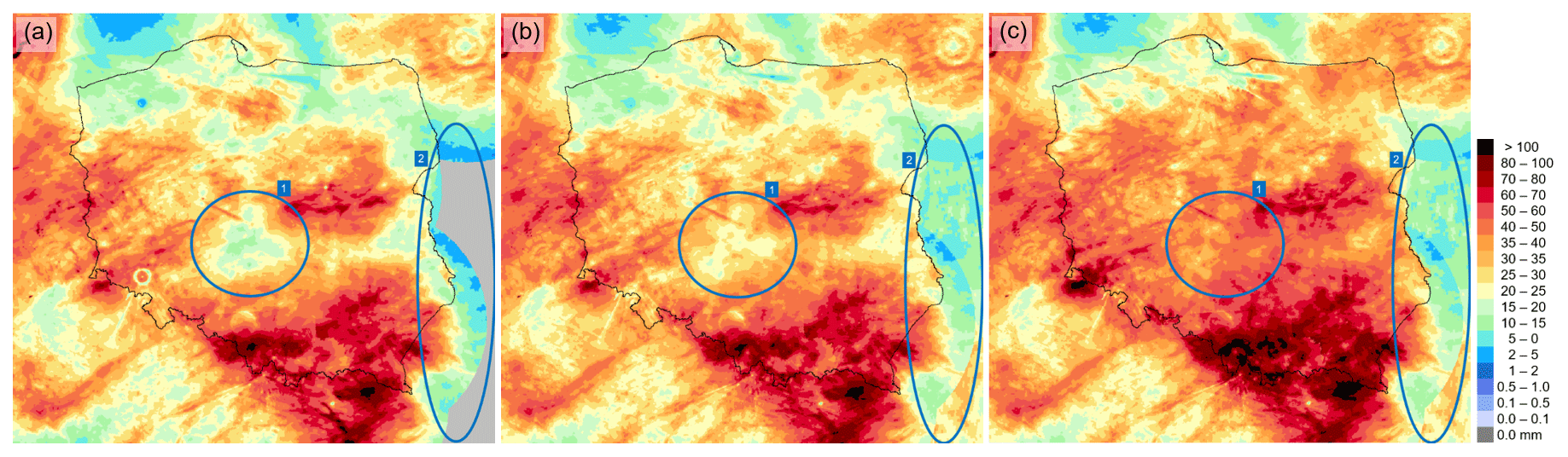
Figure 7 Fields of monthly precipitation accumulations: (a) GRS_real−time, (b) GRS_reanalysis and (c) ${\mathrm{GRS}}_{\mathrm{reanal}.+\mathrm{adj}.}$. Domain of Poland, April 2021.

The RRSE annual cycle (Fig. 5b) also shows the largest estimation errors in winter. The error is rather high in winter, at about 1.3–1.4 for GRS_real−time, and the reanalysis improved the reliability of the precipitation estimate, resulting in a decrease in the RRSE to a value of about 1.1–1.2. For the other months, the error is lower, at about 0.5 for GRS_real−time, and the reanalysis improved the reliability of the estimate to a lesser extent, as the RRSE decreased by about 0.1.

High values of RMSE (Fig. 5c) are observed in winter, when they reach 27–29 mm for GRS_real−time, but unlike RRSE, they also occur in the summer months, which is related to the frequent occurrence of intense convective precipitation during this season. They do not induce a similar increase in RRSE values because this statistic is relative as the result of dividing the RMSE by the standard deviation from the reference value (Eq. 6). Reanalysis reduces RMSE values in winter by about 5 mm per month, slightly less in the other seasons, and adjustment to manual rain gauges reduces them to about 5–10 mm per month independently of the season.

The correlation coefficient CC (Fig. 5d) is more sensitive to the existence of relationship between evaluated and reference data than the other statistics, which are based on the comparison of estimated and reference values. The CC values also indicate the lowest reliability of the precipitation estimates in winter, when the coefficient equals about 0.65 and improves to about 0.75 after reanalysis. The reason for these low values can also be explained by the low variability in the precipitation accumulations over this period, which results in a low correlation with the manual rain gauge measurements. In other seasons, especially in the summer months, the CC values are much higher, as they reach approximately 0.8–0.9 for both operational and reanalysed estimates. The adjustment to the manual rain gauges increases the correlations to approximately 0.9–0.95.

In March 2022, there was a noticeable deviation from the typical annual pattern described above for the CC coefficient. This was due to the exceptionally dry period that occurred at that time in the whole country, particularly in northern Poland. Typically, monthly precipitation accumulation for March is around 30–40 mm in Poland, but in 2022 it was significantly lower, and in the northern part of the country it was often even zero. In this case, the correlation coefficient usually increases, so in this particular month, the correlation value for vGRS_real−time was as high as 0.90, rising to 0.93 after reanalysis. Another unexpected value of the CC coefficient was observed in May 2022, when the correlation was around 0.7, which was improved by reanalysis and adjustment, after which the CC increased to around 0.95. The reason for this effect was probably a Legionowo radar replacement at that time because this radar covers a large part of the domain where other radars do not reach.

In general, the reliability of monthly estimates of precipitation field accumulation is clearly dependent on the season. Two evident phenomena can be observed here: in winter (November–February), high values of bias, RRSE and RMSE are noticeable at the same time as low values of CC, as indicated in the above analysis. In summer (July–August), the situation is different, as convective thunderstorm precipitation is often observed during this time, so the intensity of precipitation is higher, and monthly accumulations are much higher, which is also reflected in the RMSE values, while the correlation with the reference data (CC) is then significantly higher.

Table 2 summarises statistics for two selected months from 2022: January for winter and August for summer. The table shows the values of quality metrics for the three multi-source precipitation fields: operationally generated (GRS_real−time), after reanalysis (GRS_reanalysis) and after adjustment of this reanalysed precipitation field $\left({\mathrm{GRS}}_{\mathrm{reanal}.+\mathrm{adj}.}\right)$, with manual rain gauge observations as a reference. All statistics are worse for winter than for summer; however, reanalysis as well as adjustment worked much more effectively in winter. Precipitation reanalysis, involving merging individual rainfall fields for daily (instead of 10 min) accumulations along with the associated more effective data quality control, results in a clear improvement in all quality statistics in winter (January 2022), e.g. RMSE by almost 4.5 mm and CC by 0.1. In summer (August 2022), however, this impact is much smaller and amounts to less than 0.6 mm and 0.02, respectively, but bias slightly increased. The further improvement, which results from adjustment to data from manual rain gauges, is much more evident – in winter it is more than 13.5 mm in RMSE and 0.16 in CC, and in summer it is more than 11.8 mm and 0.04, respectively.

To conclude, for all the statistics used here, the improvement in the quality of monthly accumulation of estimated precipitation fields GRS_reanalysis and ${\mathrm{GRS}}_{\mathrm{reanal}.+\mathrm{adj}.}$ relative to operational fields GRS_real−time is clearly visible. The differences between the statistics of ${\mathrm{GRS}}_{\mathrm{reanal}.+\mathrm{adj}.}$ and GRS_real−time are much larger. This is mainly due to the fact that, in the absence of any other possibility, the verification was carried out using data from manual rain gauges as a reference, and here they are dependent data, as they are used during the generation of the final ${\mathrm{GRS}}_{\mathrm{reanal}.+\mathrm{adj}.}$ (see point 7 in the data-processing scheme in Sect. 4.2).

Figure 6 shows graphs of the relationship between the estimated fields of monthly accumulated RainGRS precipitation calculated operationally (generated in real time), after reanalysis and after adjustment of this reanalysed precipitation field, and monthly accumulations observed by manual rain gauges, for the same two months for which the values of statistics are summarised in Table 2. The graphs show precipitation values at locations of manual rain gauges. The correlation for the GRS_reanalysis estimate compared to GRS_real−time improved, although only slightly. This conformity, measured by the distance between the trend line (red) and the 1 : 1 line (dashed), clearly improved in winter but declined slightly in summer. The conformity with manual rain gauges for the ${\mathrm{GRS}}_{\mathrm{reanal}.+\mathrm{adj}.}$ estimate is clearly greater than that for the GRS_reanalysis, but it should be borne in mind that the data from manual rain gauges are not fully independent. Nevertheless, this comparison gives some information about the effectiveness of the final step in generating precipitation field estimates with the RainGRS Clim system.

6 Example of a climatological estimate of monthly precipitation accumulation

In Fig. 7 we can see an example of estimates of monthly precipitation accumulations for the domain of Poland, 900 km × 800 km (see Fig. 2). From the left there are estimates: operational, after the reanalysis, and after reanalysis and adjustment to manual rain gauge data. In general, values of the estimated precipitation increased after the reanalysis as a result of the more effective performance of the merging algorithm for longer accumulations. After the adjustment to manual rain gauges, the further, much higher increase in the precipitation values is because radar-based precipitation estimates are underestimated in the case of Polish weather radars. Moreover, it should be taken into account that rain gauges also underestimate rainfall because they are mostly tipping-bucket devices (Segovia-Cardozo et al., 2021).

The area of underestimated precipitation in the centre of Poland marked with “1” in Fig. 7 is the place where the distance to the closest radar site is longest – more than 200 km, where the radar beam passes over part of the precipitation (overshoots). Moreover, the telemetric rain gauge network is rather sparse here. Adjustment to manual rain gauges has made it possible to correct this underestimation.

The area denoted “2” in Fig. 7 indicates the region where there are no radars, even from neighbouring countries. Reanalysis partially improves it by complementing the lack of data with satellite-based precipitation but not wholly effectively due to the higher uncertainty in the satellite estimates.

7 Conclusions

The following general conclusions can be drawn about the proposed methodology for the generation of long-term precipitation estimates by the RainGRS Clim system:

1. Based on an analysis of available precipitation data, it was assumed that the most reliable precipitation measurement technique is a network of manual rain gauges. In particular, it was assumed that these measurements are unbiased. Since their daily accumulations are available with a long delay due to their transfer and manual quality control, they cannot be used in real time, but they can be used effectively to perform adjustment of reanalyses (see Sect. 5.2 and 5.3).

2. The second major limitation of manual rain gauges is that they only provide point observations. However, the relatively high density of this measurement network in Poland (Fig. 1) makes them very useful in the adjustment of other precipitation field estimates.

3. With daily accumulations, which, due to the time step of manual rain gauge measurements, are the basic accumulations in the algorithm for generating climatological precipitation estimates described in Sect. 4.2, it becomes possible to perform much more effective quality control, particularly in terms of removing various types of artefacts in weather radar data.

4. Algorithms for merging rain gauge, weather radar and satellite data perform much more effectively for daily totals than for 10 min totals. This is mainly due to the fact that longer accumulations of precipitation are more consistent, as in these cases time inconsistencies between different measurement techniques play a much smaller role. In addition, with longer accumulations, errors of a random nature are more averaged out (see Sect. 4.1).

5. The results presented in the paper show that after reanalysis, estimates of the precipitation field are of higher reliability than operationally generated estimates. Adjustment of the data after reanalysis to data from manual rain gauges resulted in a further, much higher quality improvement (Sect. 5.2 and 5.3). However, it should be kept in mind that the final estimates are obtained using data from manual rain gauges, so the results of the verification performed on these data, which in this case are partially dependent, should be treated with caution.

6. Having estimates of precipitation accumulated over longer time intervals in RainGRS Clim, such as monthly intervals, creates the possibility of applying them to climatological analyses. They provide valuable information, especially when high spatial resolution of precipitation data is important.