Atmospheric boundary layer height from ground-based remote sensing: a review of capabilities and limitations

The atmospheric boundary layer (ABL) defines the volume of air adjacent to the Earth's surface for the dilution of heat, moisture, and trace substances. Quantitative knowledge on the temporal and spatial variations in the heights of the ABL and its sub-layers is still scarce, despite their importance for a series of applications (including, for example, air quality, numerical weather prediction, greenhouse gas assessment, and renewable energy production). Thanks to recent advances in ground-based remote-sensing measurement technology and algorithm development, continuous profiling of the entire ABL vertical extent at high temporal and vertical resolution is increasingly possible. Dense measurement networks of autonomous ground-based remote-sensing instruments, such as microwave radiometers, radar wind profilers, Doppler wind lidars or automatic lidars and ceilometers are hence emerging across Europe and other parts of the world. This review summarises the capabilities and limitations of various instrument types for ABL monitoring and provides an overview on the vast number of retrieval methods developed for the detection of ABL sub-layer heights from different atmospheric quantities (temperature, humidity, wind, turbulence, aerosol). It is outlined how the diurnal evolution of the ABL can be monitored effectively with a combination of methods, pointing out where instrumental or methodological synergy are considered particularly promising. The review highlights the fact that harmonised data acquisition across carefully designed sensor networks as well as tailored data processing are key to obtaining high-quality products that are again essential to capture the spatial and temporal complexity of the lowest part of the atmosphere in which we live and breathe.

1 Introduction

The atmospheric boundary layer (ABL) is the lowest part of the atmosphere where most of the interactions between the Earth's surface and the atmosphere take place (Seibert et al., 1998). It plays a crucial role for the exchange of momentum, heat, humidity, and aerosols as well as greenhouse and other atmospheric gases (Palmén and Newton, 1969; Garratt, 1994; Stull, 1988). Improved process understanding and quantitative knowledge of ABL dynamics are hence crucial for a wide range of applications with high societal, economic, and health impacts, including the assessment of air quality (e.g. Han et al., 2009; Stirnberg et al., 2021; Sujatha et al., 2016) or greenhouse gases (e.g. Lauvaux et al., 2016), the generation of renewable energy (e.g. Peña et al., 2016), numerical weather prediction (NWP; e.g. Illingworth et al., 2019), sustainable urban planning (e.g. Barlow et al., 2017), and all aspects of transportation such as aviation, shipping, or road safety (e.g. Vajda et al., 2011).

Sampling the ABL vertical profile has historically been mostly achieved using radiosondes. While these balloon ascents provide indispensable information, their temporal resolution is usually insufficient to capture the full diurnal evolution of the ABL dynamics and the significant horizontal drift of the balloon during the ascent means observations are affected by spatial variations in ABL dynamics which can be challenging for data analysis and interpretation. In recent decades, ground-based remote sensing has started to close this gap, providing high-resolution information, initially with a focus on the lowest kilometre of the atmosphere (see reviews by, e.g., Wilczak et al., 1997; Emeis et al., 2008). Significant advances in ground-based remote-sensing measurement technology and algorithm development now allow for continuous profiling of the entire ABL vertical extent (ranging from a few tens of metres to > 3 km or even higher, depending on geographic settings and synoptic conditions) at high temporal and vertical resolution (Illingworth et al., 2019; Cimini et al., 2020) and automatic detection of ABL sub-layer heights from different atmospheric quantities (Collaud Coen et al., 2014; Duncan et al., 2022).

With dense ground-based remote-sensing networks emerging in Europe and other parts of the world, it is vital to recap capabilities and limitations of the various instruments and analytical approaches to support careful network design, algorithm implementation, and sound interpretation of the results. In their recent review Zhang et al. (2020) stress that interpretation of ABL height data should always take into account the specifics of both the retrieval algorithm (e.g. which atmospheric variable is analysed?) and the input data (e.g. characteristics of the sensor used for data acquisition).

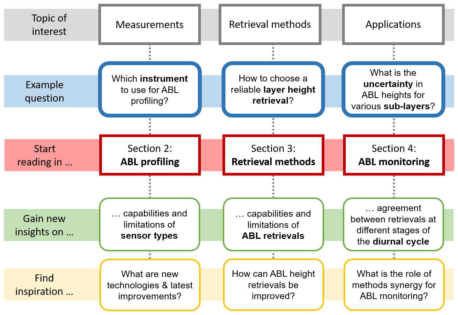
Figure 1 Entry points to this paper. The reader is invited to consult the respective section(s) related to their field of interest.

The objective of this review is to provide a general overview on the latest ABL profiling techniques while making relevant details easily accessible. The sections hence offer multiple entry points (Fig. 1) catering to a range of user backgrounds. The different atmospheric variables routinely analysed to gain insights on the ABL are presented in Sect. 1. Sensor types commonly used for ABL profiling are introduced in Sect. 2, highlighting their respective capabilities and limitations as well as their deployment in organised sensor networks. The wide range of ABL height retrieval methods is then reviewed in Sect. 3, linking potential retrieval errors to uncertainties inherent in the observed atmospheric quantity where appropriate. Quantification of layer height uncertainties is challenging, particularly due to the absence of an “absolute truth” concept that could serve as the reference standard. Section 4 outlines how the various layer height retrievals based on different atmospheric quantities compare throughout the ABL diurnal evolution and depending on atmospheric stability or cloud conditions. This is to support a data user's assessment of how well a certain layer height product may characterise their process of interest.

Ground-based profile remote sensing is a powerful tool to enhance our understanding of the atmospheric boundary layer. With careful, harmonised measurement network operations and processing procedures, increasingly detailed information can be collected to effectively support many high-impact applications. The conclusions (Sect. 5) emphasise which aspects of data acquisition, algorithm development, data analysis, and applications require additional attention to best advance this area with respect to scientific research, sensor development, and environmental monitoring operations.

The atmospheric boundary layer and its sub-layers

The ABL (synonymous with the term planetary boundary layer – PBL – which is also commonly used) is the lowest part of the troposphere where direct interactions with the Earth's surface (land and sea) take place (Seibert et al., 2000). It responds directly to surface forcings at timescales of less than 1 h (Garratt, 1994), while indirect effects (e.g. in the residual layer) can extend to daily timescales. Exchange mechanisms include the transfer of momentum, radiation, heat, moisture, particles, and gases. The ABL defines the volume in which heat, moisture, and trace substances are primarily dispersed following either the release at the surface or some altitude within the ABL or the entrainment from the free troposphere (FT) above. Exchanges with the FT take place via entrainment and ejection processes (Stull, 1988). Horizontal variations in ABL dynamics stem from a combination of synoptic atmospheric conditions (e.g. atmospheric stability, wind shear, cloud dynamics) and surface forcings (driven by contrasts, for example, in surface cover, roughness, topography) (Garratt, 1994; Seibert et al., 2000).

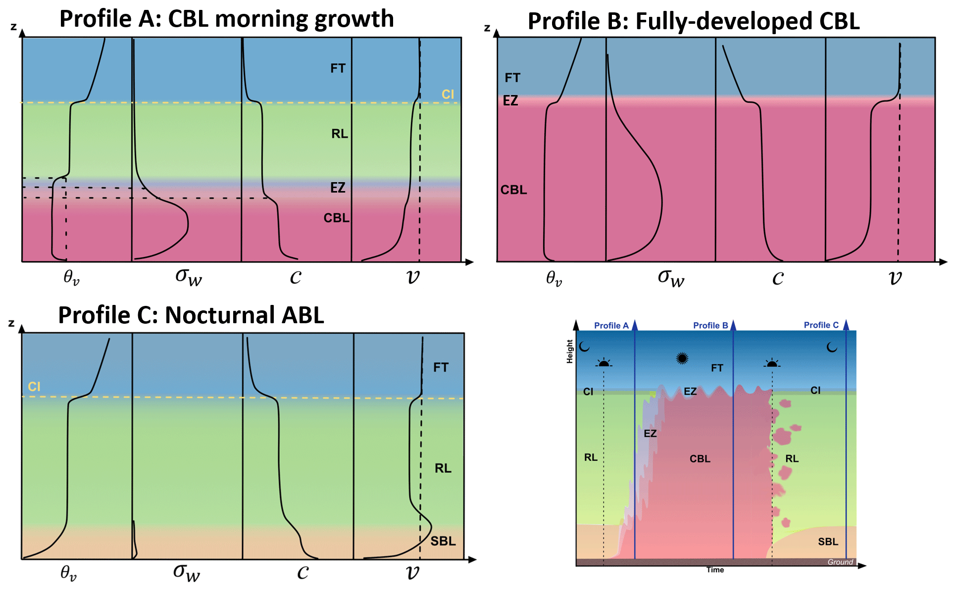
Figure 2 Idealised vertical profiles of exemplary atmospheric variables that are used to characterise thermodynamics (mean virtual potential temperature θ_v), dynamic and turbulent processes (vertical velocity variance σ_w, mean horizontal wind speed v), and resulting distributions of atmospheric tracers (mean atmospheric constituent c) during the idealised diurnal evolution of the atmospheric boundary layer (ABL), which is illustrated in the time–height sketch for an ABL over flat terrain on a cloud-free day. Dashed vertical lines in the v panels represent the geostrophic wind reference. Selected profiles are shown at three distinct moments: Profile A, the morning growth of the convective boundary layer (CBL; pink shading); Profile B, early afternoon with a fully developed CBL; and Profile C, nocturnal conditions with a residual layer (RL; green shading) above the stable boundary layer (SBL; orange shading) near the surface. A capping inversion (CI) separates the ABL from the free troposphere (FT; blue shading) above. The entrainment zone (EZ) is a region of enhanced exchange between the CBL and the RL or FT, respectively. As the morning growth of the CBL (Profile A) is associated with high temporal variability of temperature, turbulence, and atmospheric constituents in the EZ, the temperature inversion, the reduction in vertical turbulent activity, and the vertical decrease in atmospheric constituent concentration may not always be located at the same height above ground, which is indicated by slightly changing colours and horizontal dashed lines. Idealised profiles and ABL sub-layer evolution adapted from De Wekker and Kossmann (2015), Beyrich (1997), and Stull (1988).

The height of the ABL (ABLH) is here considered to be the height above ground where the surface influence becomes low, i.e. the transition to the FT. Different sub-layers occur within the ABL depending on atmospheric stability. If surface-driven processes dominate over synoptic flow conditions on a warm, cloud-free day, the ABL tends to follow a textbook evolution (Fig. 2) with a convective boundary layer (CBL) forming in the morning in response to solar heating of the ground and resulting turbulent heat fluxes. The height of the CBL (CBLH) increases during the morning and reaches its peak in the early afternoon when it extends over the whole ABL (ABLH = CBLH). Around sunset, radiative cooling of the surface induces the growth of a new layer near the ground, the stable boundary layer (SBL). At this time of reduced solar input and decaying buoyancy, the CBL breaks down and decouples from the surface, thereby being converted into the residual layer (RL), now located above the SBL top (SBLH). The height of the RL (RLH) now coincides with the ABLH (ABLH = RLH). On the following day again, the RL is usually entrained into the newly forming CBL during morning growth. While neutral atmospheric stability usually dominates the RL, it is less frequent near the surface (Collaud Coen et al., 2014) but may still occur when shear production of atmospheric turbulence is strong (Nieuwstadt and Duynkerke, 1996).

In response to surface–atmosphere exchanges, cloud processes or synoptic-scale dynamics, the ABL sub-layers can deviate from this idealised concept. For example, over complex terrain, multiple layers often form in response to different mechanisms driving the ABL dynamics (De Wekker and Kossmann, 2015; Serafin et al., 2018). In cold seasons or over cold surfaces (such as snow and ice), the SBL can also dominate during daytime, leading to an absence of the RL and consequently ABLH = SBLH during both day and night. In the presence of a low-level jet (LLJ), the jet core (peak wind speed) defines the top of the surface-based shear layer acting as an upper bound for turbulent transport (Banta et al., 2006; Mahrt et al., 1979). The vertical profile of air temperature in the SBL often shows a characteristic surface-based temperature inversion (SBI), whose height (SBIH) can be very meaningful in restricting vertical dilution. While vertical mixing mainly occurs in the lower levels of the temperature inversion, a combination of potential other processes such as radiative cooling, subsidence, or horizontal advection shapes the depth and the magnitude of the SBI.

But unstable conditions may also persist at night where the surface remains relatively warm even after sunset (e.g. urban areas; Barlow, 2014; Barlow et al., 2015; Pal et al., 2012). In this case, no SBL is present at night. Still, a shallow mixing layer may form around sunset (decoupled from the RL) as the nocturnal surface buoyancy is now only driven by storage and anthropogenic heat fluxes and is hence weaker than the mixing during daytime. In this review, the term mixing boundary layer (MBL) generally refers to the ABL sub-layer closest to the ground. Its height (MBLH) may indicate either CBLH or SBLH, whichever is present at the given moment. The MBLH terminology is applied when no information on atmospheric stability is available to differentiate between SBL and CBL.

Exchange between the CBL and the FT (or the RL) occurs via the penetration of the CBL thermals into the air aloft and the entrainment of relatively warm and (in the absence of clouds) dry air into the CBL. As horizontal wind speeds are usually lower in the CBL compared to the FT or RL (Fig. 2), wind shear at the CBLH further generates mechanical turbulence that contributes to the entrainment. The entrainment zone (EZ) refers to this region of interaction around the CBLH, and its depth (EZD) is related to the contrasts between the air in the CBL and the above FT (or RL). The ABL transition to the FT is marked by a strong, positive temperature lapse rate, the capping inversion (CI). EZD is greater when the temperature difference between ABL and FT is weak (AMS, 2017). The CI often coincides with a sharp vertical decrease in specific humidity and significant vertical wind shear (Fig. 2). The EZ is associated with temporally intermittent turbulence and a vertical decline in intensity of the turbulence (Gryning and Batchvarova, 1994). The ABL–FT exchanges are increasingly important over heterogeneous surfaces or complex topography (Lehning et al., 1998).

The interaction of clouds and ABL dynamics depends on the cloud type (Harvey et al., 2013). Cumulus clouds (Cu) forming at the CBL top can be understood as generating a deep EZ, and, thus, the ABLH is located above the cloud-base height, i.e. somewhere within the Cu. Radiative cooling in stratocumulus clouds (Sc) induces top–down mixing from the cloud layer toward the surface during day and night (Hogan et al., 2009; Wood, 2012) so that ABLH is more likely to coincide with the cloud top. If deep convective clouds are present, e.g. cumulonimbus (Cb) before the occurrence of precipitation, the ABL may present higher relative humidity, greater instability, stronger temperature inhomogeneity, and less wind shear (Zhang and Klein, 2010) so that it becomes challenging to define the ABLH.

Layers of gaseous species or aerosols (e.g. dust, smoke, ash) can be present in the FT, e.g. through long-range transport, volcanic eruptions, or pyrocloud convection (Fromm et al., 2010; Lareau and Clements, 2016). The lofted layer may remain decoupled from the local ABL but can also be (partially) entrained (Granados-Muñoz et al., 2012; Bravo-Aranda et al., 2015).

2 Atmospheric boundary layer profiling

As stated by Beyrich (1997), profile observations should fulfil a series of requirements to adequately support the assessment of ABL dynamics and the detection of layer heights. Specifically, they should (i) cover the full extent of the ABL (from the ground to the FT), (ii) have high vertical resolution of about 10–30 m, (iii) high temporal resolution of ≤ 1 h, and (iv) describe either the mixing itself or a result of mixing processes. We add that data with high temporal coverage (e.g. long time series) are necessary to determine variations in ABL dynamics at different temporal scales (synoptic, seasonal, annual, inter-annual), and measurements at multiple geographic locations enable horizontal variations to be assessed. Adequate atmospheric profiles (Sect. 2.1) can be captured by a series of different technologies (Sect. 2.2) that are increasingly operated in coordinated measurement networks (Sect. 2.3).

2.1 Profile variables characterising the atmospheric boundary layer structure

Different quantities provide insights into ABL dynamics and can be analysed to derive the heights of the various sub-layers (Sect. 1). While thermodynamic variables capture atmospheric stability conditions at a given moment, dynamic variables describe the mixing processes induced by this stratification, and tracer variables may portray the result of recent mixing processes (Table 1). Figure 2 indicates how vertical profiles of selected exemplary atmospheric variables evolve throughout the idealised evolution of the ABL on a cloud-free day.

Table 1 Atmospheric variables analysed for the detection of ABL heights are relevant for thermodynamic and dynamic processes or act as atmospheric tracers. Measurement variables provide information on the probed atmosphere but are strongly dependent on sensor characteristics or measurement setup. Depending on the measurement technology, variables are directly observed, retrieved from measurements or calculated. Note: humidity can also be interpreted as an atmospheric tracer but is here grouped with air temperature due to its importance for thermodynamic processes. Based on the variables listed here, other higher-order variables or parameters can be calculated (such as turbulent fluxes or Richardson numbers) that are valuable for characterising the ABL, for example where observations from multiple systems are available for synergy applications.

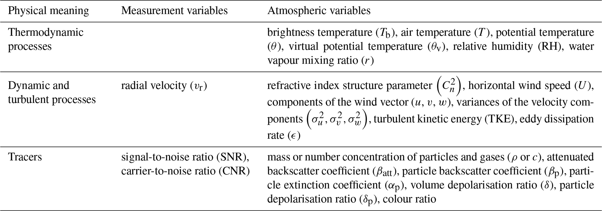
These variables can either be measurement variables that are somewhat defined by the observation technology and setup (e.g. radial velocity obtained by a Doppler wind lidar along its laser line of sight; Sect. 2.2.3) or atmospheric variables that describe a physical process or characteristic of the air rather independently of the observation technique. Some atmospheric variables are output directly by a certain sensor (e.g. air temperature measured with an in situ thermometer of a radiosonde; Sect. 2.2.1), while others are retrieved during post-processing following methods of various complexity. Certain variables are calculated as a combination of multiple variables (e.g. potential temperature calculated from air temperature and atmospheric pressure, colour ratio determined from backscatter coefficient observed at two different wavelengths) or by applying higher-order statistics (e.g. variance of vertical velocity) or both (e.g. turbulent kinetic energy calculated from variances of the three wind velocity components). Other variables require more complex retrieval algorithms, with a series of assumptions (e.g. retrieval of wind speed components from Doppler radial velocity) and even auxiliary information (e.g. retrieving air temperature from microwave radiometer brightness temperature).

Both atmospheric variables and measurement variables can be exploited for ABL height detection (Sect. 3). Those most commonly utilised can be grouped by their physical relation to ABL dynamics (Table 1).

2.2 Measurement principles

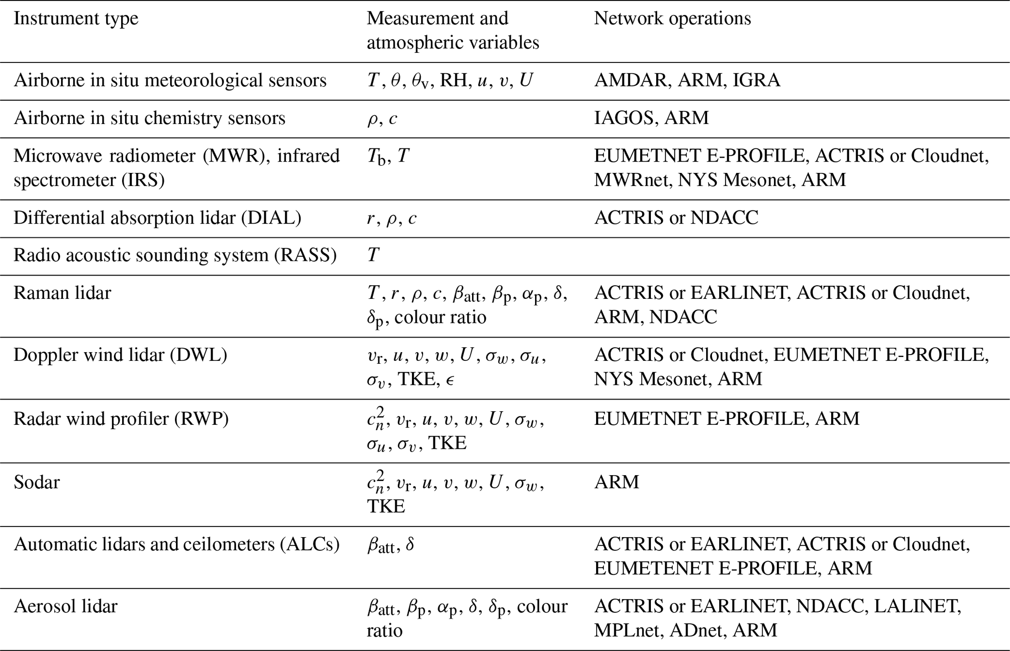
A range of technologies (Table 2) is available to measure the quantities (Sect. 2.1) analysed for layer detection (Sect. 3). Atmospheric profile measurements can be achieved using tower-based or airborne in situ sensors (Sect. 2.2.1) or with remote-sensing techniques that again can be airborne, spaceborne, or ground-based. Ground-based remote-sensing profilers generally provide data at high temporal and vertical resolution and good sensitivity in the ABL. In the following, sensors are briefly introduced, grouped according to their characteristic output variables into profilers for thermodynamic variables or atmospheric trace gases (Sect. 2.2.2), wind and turbulence profilers (Sect. 2.2.3), and aerosol profilers (Sect. 2.2.4). For further technical details, the reader is referred to relevant textbooks (e.g. Emeis, 2010; Foken, 2021).

Table 2 Instrument types used to gather vertical profiles of atmospheric and measurement variables (Sect. 2.1; Table 1) in the atmospheric boundary layer. These observations are increasingly organised in national and international monitoring networks (see Sect. 2.3 for further details). Abbreviations: ACTRIS (Aerosols, Clouds and Trace gases Research Infrastructure), ADnet (Asian Dust and aerosol lidar observation network), AMDAR (Aircraft Meteorological Data Relay), ARM (Atmospheric Radiation Measurement), EARLINET (European Aerosol Research Lidar Network), EUMETNET E-PROFILE (European Profile of the European Meteorological Network), IAGOS (In-service Aircraft for a Global Observing System), IGRA (Integrated Global Radiosonde Archive), LALINET (Latin America Lidar Network), MPLnet (NASA Micro-Pulse Lidar Network), MWRnet (Microwave Radiometer Network), NDACC (Network for the Detection of Atmospheric Composition Change), NYS Mesonet (New York State Mesonet).

While passive radiometer technologies capture thermodynamic profiles (Sect. 2.2.2), most remote-sensing approaches actively emit a signal which is then recorded after its interaction with the probed atmospheric volume. Probably the most widely applied approach for ground-based atmospheric remote sensing is using laser technology. Depending on the instrument specifics, lidars can be used to measure profiles of meteorological properties such as wind and turbulence (e.g. Doppler lidars), temperature (e.g. Raman lidars), humidity (e.g. differential absorption lidars), atmospheric gases (e.g. other inelastic lidars), or atmospheric aerosol particle characteristics (e.g. aerosol backscatter lidars). For all lidar systems, the incomplete optical overlap between the field of view of the receiver telescope and the emitted laser beam (Freudenthaler et al., 2018; Simeonov et al., 1999) can significantly increase the uncertainty in the first range gates. The part of the profile affected often extends over several hundred metres, but this varies significantly with instrument design (Haeffelin et al., 2012; Caicedo et al., 2020), and also the maximum range from which the signal can be recorded depends on the instrument specifics (e.g. laser power, optics). In general, there is an inverse relation between the near-range and far-range capabilities of a given lidar system. While high-power systems have a monitoring range of many kilometres (some reaching the stratosphere), they require an increasingly large telescope which then increases the blind zone near the sensor. Low-power systems tend to have better performance in the near range but with a more limited vertical extent. While the vertical resolution of the recorded profile also tends to technically increase with laser power and vertical range extent, manufacturers increasingly apply oversampling procedures to the data products, which leads to a higher number of range gates. Thick water clouds fully attenuate the lidar signal, so that the recorded information reduces to noise at some depth inside the cloud. Furthermore, noise levels increase due to the background signal induced by solar radiation.

While ground-based techniques are the focus of this review, some ABL information can be gathered by spaceborne technologies, including aerosol lidars (e.g. Cloud–Aerosol Lidar and Infrared Pathfinder Satellite Observations (CALIPSO); Jordan et al., 2010; J. Liu et al., 2015; Zhang et al., 2016), Doppler wind lidars (e.g. Atmospheric Laser Doppler Instrument (Aeolus-ALADIN); Straume et al., 2020; Flamant et al., 2016), or radio occultation systems (Global Navigation Satellite System Radio Occultation (GNSS-RO); von Engeln et al., 2005; Ao et al., 2012; Xie et al., 2012; Chan and Wood, 2013; Basha and Ratnam, 2009). Satellite microwave and near-infrared passive observations also allow for the quantification of boundary layer water vapour even beneath uniform marine clouds (Millán et al., 2016). Following the success of COSMIC, the promising COSMIC-2 mission was launched in 2019 to provide radio occultation data at an even higher resolution through deeper tropospheric penetration (50 % within 200 m of Earth's surface). These observations enable improved detection of the ABLH and super-refraction at the top of the ABL (Ho et al., 2020; Schreiner et al., 2020). Satellite observations are less applicable for the detection of very shallow layers (e.g. Aeolus-ALADIN is not suitable for the monitoring of shallow layer conditions; Abril-Gago et al., 2021) or sub-layer heights (such as SBLH and RLH) given the degradation of profiles at low altitudes above the surface (Seidel et al., 2010; Xie et al., 2012) and the relatively coarse horizontal resolution (e.g. ∼ 200 km for GNSS-RO and ∼ 87 km for Aeolus). The latter introduces additional uncertainty over coastal regions as well as in the presence of complex terrain (Ao et al., 2012). Still, satellite-based ABL heights are very valuable, as they provide globally consistent estimates (Ho et al., 2015) whose seasonal cycle constitutes an important constraint on the behaviour of global atmospheric models (Chan and Wood, 2013; J. Liu et al., 2015).

In the following sections the emphasis is placed on in situ platforms and ground-based remote-sensing instruments that are to date commonly used to observe the ABL and can be considered the most promising candidates for extensive measurement network operations (Sect. 2.3). These are radiosoundings for in situ profiling (Sect. 2.2.1; note that significant advances are expected for network operations of uncrewed aerial systems), passive radiometers for temperature profiling (Sect. 2.2.2), Doppler wind lidars for profiling of wind and turbulence (Sect. 2.2.3), and finally automatic lidars and ceilometers for aerosol profiling in the ABL (Sect. 2.2.4).

During the discussion of respective sensor capabilities, it is obviously of interest to assess the agreement of observations obtained from different sensors in terms of absolute values. However, it should be kept in mind that layer height retrieval methods (Sect. 3) tend to exploit relative changes (such as vertical gradients), which means aspects such as sensor response time of in situ instruments or vertical resolution are generally also critical to consider.

2.2.1 In situ profiling

In situ sensors are attached to various kinds of platforms to gather atmospheric profile measurements. Instruments operated at multiple levels on tall towers are capable of capturing conditions in the lowest few hundred metres of the atmosphere based on profiles of temperature, humidity, wind, turbulence or atmospheric composition (Bosveld et al., 2020; Ramon et al., 2020; Neisser et al., 2002), often continuously at very high temporal and vertical resolution. A similar range of the atmospheric column can be probed by instruments hosted on tethered balloons (Keller et al., 2011; Spirig et al., 2004); however, the latter are still mostly operated manually during dedicated field campaigns only.

Other airborne measurements of meteorological variables and atmospheric composition tend to reach higher atmospheric levels, including in situ sensors attached to radiosonde balloons or on board of aeroplanes. Radiosondes are probably the most common data source used to derive ABLH operationally. In situ measurements of air temperature and humidity are taken by sensors that are being lifted up by a helium-inflated aerostatic balloon, while atmospheric pressure, wind speed, and direction are derived along the flight path via satellite tracking (e.g. GPS). The balloon ascent allows profiles to be recorded up to ∼ 35 km above ground level (a.g.l.) with high and nearly constant vertical resolution of the order of tens of metres. The sounding takes 1.5–2.0 h to reach the maximum altitude before the balloon bursts (usually in the lower stratosphere). Typical uncertainties in radiosonde measurements are ±0.2–0.6 K for air temperature, 6 % for relative humidity, and 0.4–1.0 m s⁻¹ for horizontal wind speed (Bian et al., 2011; Dirksen et al., 2014; Renju et al., 2017). Lightweight sondes attached to smaller balloons (Bessardon et al., 2019) are not always able to profile the entire troposphere; however, they usually ascend to heights above the ABLH. As they are technically easier to operate and may not require the same level of security clearance they are particularly useful for ABL profiling in populated environments such as cities.

The main advantages of radiosonde data are the following: (i) observations of temperature, humidity, air pressure, wind speed, and direction are collected simultaneously using the same measurement system; (ii) coordinated radiosonde ascents are available at a high number of launch sites worldwide (Sect. 2.3); (iii) data are transmitted via international communication networks with a very short time delay which makes them well-suited for operational use; and (iv) time series extend for decades, making radiosondes especially valuable for climatology studies. It should be noted, however, that only 177 sites worldwide (status 2021) meet the stringent requirements for climate monitoring (WMO, 2018; Thorne et al., 2017; WMO, 2010).

The main shortcoming of radiosondes is their low temporal frequency. Most operational sites only launch the balloons twice daily at specified synoptic times (00:00, 12:00 UTC), with some up to four times daily. While these coordinated launches at synoptic times are required to take the extremely valuable global snapshot of the atmosphere, they generally limit the representation of the ABL diurnal evolution at a given place. Where the launch times occur, e.g. during morning growth and/or evening decay of the CBL, diurnal minima or maxima may not be captured. Even during special field campaigns, 1.5–3.0 h is typically the closest interval between launches. This low temporal resolution hampers the investigation of the diurnal cycle of ABL sub-layer heights and the comparison of ABLH maxima at different locations. Note that some radiosonde data products of routine ascents limit the vertical information to standard, significant pressure levels for real-time dissemination and archiving. This often means details of the ABL structure are obscured.

Another specific problem that can result in systematic errors in derived ABL characteristics stems from the significant horizontal displacement of the balloon during the ascent (Schween et al., 2014). This drift means observations are affected by spatial variations in ABL dynamics, which can be challenging for data analysis and interpretation. In addition, humidity sensor uncertainties in cold and dry or cloudy conditions (Seidel et al., 2010; Wang and Wang, 2014) can cause errors. Some stations operate automatic launch systems that can introduce temperature and humidity uncertainties in the lowest altitudes (< 200 m) as sondes are located in climate-controlled chambers before being released into ambient air (Madonna et al., 2020). Site-dependent radar tracking uncertainties (Seibert et al., 2000) that have, in the past, caused errors in the wind profiles at low altitudes are no longer a concern as GPS tracking is now used instead. Careful removal of discontinuities induced by changes to the operating system helps to harmonise long-term records (Madonna et al., 2022).

Uncrewed aerial systems (UASs) can gather data at very high temporal and vertical resolution often covering the full vertical extent of the ABL; however, they cannot (yet) be operated fully autonomously and temporal coverage is often limited. Similarly, data from research aircraft flights (e.g. Guimarães et al., 2019) are scarce. The air volume sampled by both UASs and research aircraft flights can be restricted by air traffic control regulations. Networks of commercial passenger aeroplanes gather atmospheric profile information more continuously. The WMO system Aircraft Meteorological Data Relay (https://public.wmo.int/en/programmes/global-observing-system/amdar-observing-system, last access: 23 December 2022; AMDAR) and the European Research Infrastructure In-service Aircraft for a Global Observing System (https://www.iagos.org/, last access: 23 December 2022; IAGOS) collect several atmospheric variables (such as temperature, humidity, wind speed, wind direction, or various atmospheric constituents, depending on the measurement system) during their flights, thereby gathering vertical ABL profile data near the airports during start and landing. Observation accuracy is generally similar to that of radiosondes (Berkes et al., 2017); however, the vertical resolution is lower and systematic biases have been reported (e.g. AMDAR air temperature bias of up to 0.5–1.0 K; Ballish et al., 2008). Further, the aeroplane flight paths are associated with a much greater horizontal displacement (∼ 10 km km⁻¹) than radiosondes (∼ 1 km km⁻¹; Rahn and Mitchell, 2016). Naturally, the temporal resolution of IAGOS and AMDAR profiles depends on the frequency of reporting aeroplanes starting or landing in the region of interest. AMDAR data have been applied successfully to study the ABL in regions with multiple busy airports in close vicinity, such as Los Angeles, USA (Rahn and Mitchell, 2016), London, UK (Kotthaus and Grimmond, 2018a), or Paris, France (Kotthaus et al., 2020), while Petetin et al. (2018) derive generalised ABL profiles for Northern Hemisphere midlatitudes from a climatology of IAGOS profiles.

2.2.2 Profiling of thermodynamic variables and atmospheric gases

Different ground-based remote-sensing technologies are available to obtain vertical profiles of thermodynamic variables (temperature, water vapour) and/or other atmospheric gases. These include Raman lidars, differential absorption lidars (DIALs), radio-acoustic sounding systems (RASSs), and radiometers.

Raman lidar systems transmit at one or multiple wavelengths and detect the Raman-shifted scattering by molecular excitation at other wavelengths, enabling the determination of the constituent of interest (Table 2), such as the water vapour mixing ratio (Wulfmeyer et al., 2010), the particle extinction coefficient (Ansmann et al., 1992), or air temperature using the rotational Raman technique (Behrendt et al., 2015). Raman lidars widely use Nd:YAG lasers at tens of hertz typical repetition rates, with an extremely high pulse energy of > 1 J at the fundamental wavelength (1064 nm) and up to hundreds of millijoules (mJ) at the second (532 nm) and third (355 nm) harmonics. Depending on the laser repetition rate and pulse energy, temporal resolution ranges from seconds to minutes. Range resolution is defined by the speed of the data acquisition system (e.g. a 100 ns laser pulse length has a 15 m folded scattering length; Weitkamp, 2005), with very high resolution (< 10 m) possible. The most prominent limitation for the exploitation of Raman lidar data for ABL studies is their limited temporal coverage. These systems are generally not operated continuously because Raman channels only provide usable results when the natural background light is low, i.e. at night. In addition, consumables of high-power lidars are expensive, so that most operators limit measurements to times when no low-level liquid water clouds are present as these extinguish the lidar signal at very low altitudes. As a consequence, Raman lidars are rarely used to monitor ABL dynamics and studies focus on atmospheric layers at greater altitudes instead.

A DIAL transmits laser beams at two wavelengths exploiting the differential attenuation (Lammert and Bösenberg, 2006) to derive vertical profiles of water vapour (Behrendt et al., 2007) or trace gases such as CO₂ (Gibert et al., 2008), CH₄ (Robinson et al., 2015), ozone (Banta et al., 1998; Ravetta and Ancellet, 1998), or NO₂ (Piters et al., 2012). Thanks to recent developments, compact DIAL systems are becoming increasingly available. As they use a significantly lower pulse energy compared to the Raman lidars (Newsom et al., 2020), they can be suitable for continuous water vapour profiling of the ABL.

RASSs either combine a radar wind profiler with a source of acoustic signals (e.g. sodar) or a sodar system with a source of electromagnetic signals (Emeis, 2010; Foken, 2021). From the Doppler shift in the respective Bragg-scattered radar signal the speed of sound is measured as a function of altitude, from which the profile of virtual temperature can be deduced. The uncertainty in temperature can be <0.5 K, provided a number of careful corrections are applied (Görsdorf and Lehmann, 2000). Temporal resolution depends on the application, with 10 min averaging being typical. The vertical resolution of the profile depends on the length of the pulse transmitted, with RASSs usually configured to have a resolution of 30–60 m. As for many ground-based remote-sensing instrument types, the capabilities to capture information in the near-range or greater altitude depends on the specific RASS characteristics. While sodar-based RASSs or 1 GHz radar wind profilers with RASS capability reach their maximum range at about 500 m, measurements well above 1 km can be obtained with RASSs using a radar wind profiler at about 500 MHz.

Two types of ground-based profiling radiometers measure the downwelling radiance naturally emitted by the atmosphere at selected band channels: microwave radiometers (MWRs) and infrared spectrometers (IRSs). The measured radiance is internally converted to atmospheric brightness temperature (Table 1). As T_b holds information on atmospheric thermodynamic conditions, further atmospheric variables (e.g. temperature, humidity, liquid water path, and integrated water vapour content) can be derived, using retrieval methods aided by some a priori knowledge. The atmospheric variables obtained from MWR and IRS depend on the number and spectral range of the channels utilised by a given sensor.

In the 20–60 GHz frequency (0.5–1.5 cm wavelength) range, the atmospheric thermal radiance is mostly emitted by atmospheric gases (primarily oxygen and water vapour) and hydrometeors (mainly liquid water droplets). MWRs operating at several channels in the 20–30 and 50–60 GHz frequency bands observe temperature and humidity profiles, respectively. The vertical resolution of the obtained temperature profiles is higher in the lowest 2 km where most of the information content resides. For humidity profiles the information is spread along the vertical range with generally coarser resolution. Most of the common MWR profilers provide information on tropospheric temperature and specific humidity and the column-integrated liquid water content (Solheim et al., 1998; Westwater et al., 2004; Rose et al., 2005) at high temporal resolution (∼ 1 min). When compared to nearby radiosonde ascents, MWR retrievals agree within 0.5–2.0 K root mean square deviation (RMSD) for temperature (decreasing from surface upwards) and 0.2–1.5 g m⁻³ for absolute humidity. The mean RMSD value within the boundary layer is ∼ 0.8 K for the temperature retrievals (Liljegren et al., 2005; Cimini et al., 2006; Löhnert et al., 2009; Löhnert and Maier, 2012). Bias values between MWR and Raman lidars are within ±0.4 g kg⁻¹ (or ±20 %) for water vapour mixing ratio measurements with RMSD < 1 g kg⁻¹ (25 %–55 %) and within 0–1.2 K for temperature measurements with RMSD ∼ 0.6–1.8 K (at 5 min integration time; Di Girolamo et al., 2020). When their results are compared to radiosonde data, Bianco et al. (2017) find lower statistical differences for RASS than for MWR.

IRSs exploit high-spectral-resolution radiances measured in the thermal infrared spectrum to retrieve temperature and water vapour profiles in cloud-free air. The Atmospheric Emitted Radiation Interferometer (AERI) is a Fourier transform IRS operating in the thermal infrared range (3000–520 cm⁻¹ wavenumber, 3.3–19 µm wavelength; Knuteson et al., 2004a, b). It is specifically designed to record downwelling radiance at high spectral resolution (0.5 cm⁻¹). The observed radiance is processed to retrieve temperature and water vapour profiles up to cloud base and in addition cloud properties and trace gas concentrations (Feltz et al., 2003; Turner and Löhnert, 2014; Turner and Blumberg, 2018), with a temporal resolution of 30 s. When compared to nearby radiosonde ascents, IRS retrievals agree within ∼ 1 K RMSD for temperature and ∼ 0.8 g kg⁻¹ for water vapour mixing ratio (e.g. Blumberg et al., 2015; Wulfmeyer et al., 2015; Weckwerth et al., 2016).

Thermodynamic profiles from MWR or IRS have been demonstrated to be useful to estimate ABLH (Cimini et al., 2013) and atmospheric stability indices (Feltz and Mecikalski, 2002; Wagner et al., 2008; Cimini et al., 2015). However, despite their similarities they provide partially complementary information. In general, IRS data have greater information content than MWR, resulting in higher vertical resolution for temperature and humidity profiles, and sensitivity to trace gases and cloud particle size. IRS also provides higher sensitivity to low-cloud liquid water path, though the signal saturates above ∼ 40 g m⁻². MWRs again are only slightly affected by liquid water, which gives them an advantage in capturing profiles even within or above clouds (unlike IRS, which is limited to cloud base). Further, MWRs can be used within light precipitation (Cimini et al., 2011; Bianco et al., 2017) because the antenna is protected by a radome with hydrophobic coating and a continuous tangential airflow. Still, the above measures are generally not sufficient under moderate to heavy precipitation when the quality of retrieved profiles is degraded and hence usually excluded from analysis.

The most prominent limitation of ground-based radiometric profiling is its low to moderate vertical resolution. The information content of ground-based radiometry on the vertical distribution of atmospheric thermodynamics resides in the differential absorption of multi-frequency and multi-angle observations. However, contributions from different layers to the observed T_b (i.e. the weighting functions; Westwater et al., 2004) show significant overlap, leading to substantial redundancy in the observations. Although the retrievals of atmospheric profiles from passive instruments like MWR and IRS are usually provided on fine vertical grids (e.g. ∼ 50, 100, and 250 m at < 500, 500–2000, and > 2000 m, respectively), this spacing should not be confused with the actual vertical resolution, which by definition is the minimum distance at which differences in the vertical profile are resolved. Several methods are used to quantify the vertical resolution of radiometric profiling, for example including the degrees of freedom for signal (Löhnert et al., 2009), the inter-level covariance (Liljegren et al., 2005), or averaging kernels (Blumberg et al., 2015). Using the latter, temperature profiles show a vertical resolution varying linearly with height by a factor of ∼ 2 for MWR and ∼ 1.4 for IRS. The vertical resolution for the water vapour mixing ratio is less regular but still roughly linear with height.

To summarise, passive radiometers provide better coverage of temperature and humidity profiles compared to Raman lidars because they can gather data continuously. But DIAL systems also increasingly provide continuous profiles of water vapour or other gases in the ABL. Vertical resolution is greater for IRS at 0.5–2.0 km and greater for MWR above 4 km. IRS and MWR provide partially complementary information despite their substantial similarities, given the higher vertical information content of IRS in the ABL and the capability of the MWR to gather information within and above clouds and during light precipitation. The synergy of MWR and/or IRS with active remote-sensing technologies such as DIAL or Raman lidars can improve data quality (e.g. Turner and Löhnert, 2021; Djalalova et al., 2022), e.g. achieving a more accurate representation of the moisture gradient across the entrainment zone (Smith et al., 2021).

2.2.3 Wind and turbulence profiling

Several technologies allow for the vertical profiles of mean wind speed, direction, and turbulence to be captured (Foken, 2021), including sodars, radar wind profilers (RWPs), and Doppler wind lidars (DWLs). Where profiles of both turbulence and temperature fluctuations (e.g. from RASS; Sect. 2.2.2) are observed, profiles of turbulent heat fluxes can be obtained (Engelbart and Bange, 2002; Behrendt et al., 2020).

Sodars send out pulses of sound to probe the atmosphere. The sodar technique is based on fluctuations in the refractive index of the air (Sect. 2.1), and the amplitude of the return signal is related to the refractive index structure parameter ($C_n^{\mathrm{2}}$; Singal, 1997; Bradley, 2007). Based on this, turbulent structures in the ABL can be characterised (Emeis et al., 2008; Kramar et al., 2014; Beyrich, 1997). Compared to most other remote-sensing profiling systems, sodars have a particular advantage in being capable of sensing close to the instrument, typically within 20 m. Very shallow ABL can even be measured in challenging polar locations (Kouznetsov, 2009), especially when combined with sonic anemometers (Argentini et al., 2005). This good near-range capability goes along with a rather limited range extent to about 1 km which is linked to the absorption of sound in the air and a considerable sensitivity of the system to environmental noise. Wind and turbulence derived from sodar observations are severely affected by precipitation as the fall speed of the precipitation disturbs the signal and water on the antenna tends to further increase retrieval uncertainty. Another disadvantage is that the sound signal can often be a disturbance for humans and animals which makes it difficult to operate sodars continuously in many environments.

RWPs operate on Doppler technology, either in the very high-frequency (VHF) domain (20–300 MHz) or ultrahigh-frequency (UHF) domain (0.4–2 GHz) with boundary layer RWP usually around 1 GHz (L band). UHF RWPs are better suited for probing the ABL thanks to their higher vertical resolution and lower cost. An electromagnetic pulse is emitted towards the zenith and two to four off-zenith directions (tilted at 15^∘). The angle can be achieved with different antennas or with a single phased-array antenna. In the UHF region, the return signal intensity depends mainly on humidity and temperature gradients in the atmosphere. It is recorded and analysed in real time by the system: a succession of coherent averaging and noise filtering steps are followed by a fast Fourier transform (FFT). The frequency spectrum obtained for each range gate is characterised by four moments: noise level, signal power, spectral width, and Doppler shift. By combining the Doppler shift in the three beams, mean wind speed and wind direction are calculated at each range gate (Ecklund et al., 1988). Vertical resolution is of the order of 100–400 m, depending on the measurement setup. The main advantage of RWPs is their capability to operate under all weather conditions at moderate cost. They even provide useful information inside cloud or fog layers and when aerosol concentrations are very low, presenting an advantage over lidar systems. Large errors in RWP profile data are mostly caused by larger objects, such as birds (Lehmann and Teschke, 2008). Provided suitable scan patterns, averaging strategies, and quality control are implemented, the uncertainties and biases in RWP profiles are comparable to DWL observations. With fewer than 100 RWPs operated worldwide (Sect. 2.3), their limited number is a clear disadvantage when it comes to spatial coverage.

All DWLs exploit the Doppler shift along the line of sight, or radial, to measure the radial Doppler velocity. There are two types of DWLs: one uses the molecular backscatter component and applies narrowband spectral filters to measure the frequency shift, while the other type (heterodyne Doppler lidar) uses the aerosol–particle backscatter component and coherent mixing with a reference beam to detect the slight Doppler shift in frequency between the emitted pulse and backscattered return. Given their negligible terminal fall velocities, backscattering aerosol particles and cloud droplets are ideal tracers to track the wind motion. Ground-based commercial DWLs capable of probing the full depth of the ABL typically use the heterodyne principle. They generally operate at wavelengths between 1.5–2.0 µm, taking advantage of components developed for the telecommunication industry. Note that attenuated backscatter (Sect. 2.1) can also be retrieved from DWL observations if the instrument telescope function is accounted for (Pentikäinen et al., 2020).

Heterodyne DWLs work with continuous-wave technology or by emitting short laser pulses. The maximum range for continuous-wave DWL systems is limited to about 250 m as the range-weighting function becomes very broad beyond this distance (Kavaya and Suni, 1991). Pulsed DWL systems emit very short pulses of radiation, and the range information is obtained from the round trip time between the transmitted pulse and the received signal. Their maximum unambiguous range depends on the pulse repetition frequency (e.g. a 15 kHz pulse repetition frequency corresponds to a maximum range of ∼ 10 km) and is greater than for continuous-wave systems. Pulsed DWLs are available at different frequencies, with some providing high-resolution data only over a few hundred metres.

Pointing to nadir (zenith), the radial Doppler velocity observed from aerosol or cloud droplets is the vertical air motion w; for larger particles the observed radial Doppler velocity is the sum of the vertical air motion speed w and the fall velocity of the particles. For beams tilted away from zenith, the radial Doppler velocity contains components of both the horizontal wind and the vertical motion. Combining scans from multiple directions permits the horizontal wind components to be derived using trigonometry under the assumption of horizontal homogeneity of the wind field in the observed volume (Banta et al., 2013; Päschke et al., 2015; Teschke and Lehmann, 2017). Where multiple DWLs are deployed to sample the same volume of air, direct retrievals of the three-dimensional wind vector and its fluctuations can be obtained (Sathe and Mann, 2013). Comparisons with sonic and cup anemometers on towers or masts show that winds can be derived from DWLs with sufficient accuracy for wind energy applications (Peña et al., 2008; Pichugina et al., 2012). Under ideal conditions, the DWL precision is within the uncertainty in the anemometer measurements used as a reference (Gottschall et al., 2012).

If winds are sampled at very high temporal frequency, higher-order moments, such as velocity variances (Sect. 2.1) and even skewness, kurtosis, turbulent kinetic energy (TKE), or eddy dissipation rate (ϵ) can be determined (e.g. Cohn, 1995). Being direct measures of turbulence, TKE and ϵ are best suited for fair site and instrument intercomparisons and can be obtained from various scan strategies, including vertical stare, multi-beam, or conical scanning (Banakh and Smalikho, 1997; Banakh et al., 2010; Sathe et al., 2015; Bonin et al., 2017; Smalikho and Banakh, 2017; Yang et al., 2020) or a combination of scan types (Bonin et al., 2018). TKE can also be obtained by scanning at the specific elevation angle of 35.5^∘ (Eberhard et al., 1989). These methods usually include measurements of the wind profile to provide the horizontal length scales required (O'Connor et al., 2010). Instrument noise can play a role when measuring turbulence statistics if high-frequency variations are introduced into the signal (Tucker et al., 2009; Lenschow et al., 2000). Gravity waves and other larger-scale atmospheric motions can hamper the simple interpretation of velocity fluctuations as a proxy for turbulent motion. Methods are under development to diagnose and account for such situations (Banakh and Smalikho, 2016; Bonin et al., 2018). In general, it is crucial to assess the implications of noise filtering, sampling frequency, integration time, and measurement volume on turbulence measurements (Bonin et al., 2017; Pichugina et al., 2008). Physical quantities describing atmospheric turbulence derived from DWL observations have been successfully evaluated against data gathered by sonic anemometers on masts (Bonin et al., 2016; Bodini et al., 2018; Bonin et al., 2018), tethered balloons (Frehlich et al., 2008; O'Connor et al., 2010), radiosondes (Tucker et al., 2009), or a combination of these (Wildmann et al., 2019). For a review on pulsed DWLs including descriptions of the various scan strategies, the reader is referred to, for example, Z. Liu et al. (2019).

The intrinsic uncertainty in the measured Doppler radial velocity is directly related to the DWL carrier-to-noise ratio (Rye and Hardesty, 1993; O'Connor et al., 2010). As the latter depends on both the lidar system and the aerosol load of the atmosphere, uncertainty estimates should take into account the sampling strategy and potential instrument-specific corrections (Manninen et al., 2016; Vakkari et al., 2019). Increased uncertainties have been reported in pristine conditions such as the Arctic (e.g. Hirsikko et al., 2014). As for all lidar systems, the incomplete optical overlap of DWLs usually means data in the lowest range gates need to be treated with caution and are often discarded from analysis. For DWLs that are able to gather profiles up to several kilometres' range and are hence able to capture ABLH peaks during deep afternoon convection, this blind zone may hinder the assessment of very shallow ABL sub-layers. Here mini-DWL systems that focus on the very near range at high vertical resolution offer valuable sensor synergy. The issue of incomplete optical overlap in the near range can also be somewhat overcome by scanning DWL systems because a combination of low-level scanning strategies with higher-elevation scan patterns means wind profiles are sampled throughout the entire ABL extent (Banta et al., 2006; Pichugina and Banta, 2010; Vakkari et al., 2015).

DWLs can operate under all weather conditions at high temporal (< 1 min) and vertical (< 100 m) resolution; however, thick water clouds usually fully attenuate the signal so little information can be obtained above the cloud base. Precipitation can cause significant uncertainties in the wind and turbulence retrievals since rapid variation in terminal fall velocities for different sizes of large precipitation particles (drizzle, rain drops, ice particles) manifests itself as vertical velocity fluctuations that resemble turbulence. This imparts biases if not accounted for. Methodologies using the associated variations in the signal backscattered from precipitation particles are being developed to identify such cases. Also, rainfall on the telescope window reduces measurement accuracy.

The resolution, spatial extent, and accuracy of the retrieved wind information depends on the instrument model, the scan strategy, and the state of the atmosphere. As for aerosol lidars (Sect. 2.2.4), the strength of the backscattered signal increases with aerosol load, and relative noise levels can be high where little aerosol is present. A major advantage of DWLs with scanning capabilities is that a series of different measurement setups can be alternated to gather optimised sampling strategies for several advanced data products in quick succession. This proves valuable not only for the detection of ABL sub-layer heights but also for in-depth characterisation of ABL dynamics (Sect. 4).

2.2.4 Aerosol profiling

Ground-based lidar systems available for the profiling of aerosols differ greatly in laser power and wavelengths utilised (Foken, 2021). Generally, a differentiation can be made between high-power lidar systems and the comparatively low-power automatic lidars and ceilometers (ALCs). The latter is a collective term that refers to both ceilometers which traditionally focused on cloud-base height estimation and those backscatter lidars primarily designed to continuously provide aerosol profile information (such as micro pulse lidars; MPLs). Capabilities and limitations of high-power aerosol lidars have been outlined for the Raman lidar (see description in Sect. 2.2.2), a research-grade lidar which is able to sample water vapour and at times temperature, in addition to aerosol properties (Table 2).

ALCs are compact, simple backscatter lidars which operate at wavelengths mostly in the infrared or visible spectral region (e.g. 532, 808, ∼ 910, 1064 nm are common wavelengths). ALCs record the attenuated backscatter (Sect. 2.1) signal, which commonly needs to be absolutely calibrated during post-processing (Wiegner and Geiß, 2012; Hopkin et al., 2019). While most ALCs are monochromatic, few models with multiple wavelengths do exist. Polarisation-sensitive ALCs (P-ALCs) start to emerge that are capable of monitoring the particle depolarisation profile, providing information on the aerosol shape that can be exploited for aerosol typing. Cloud-base height is the standard output variable for all ALCs in addition to the attenuated backscatter profiles. Retrievals of ABL heights are also increasingly incorporated by the manufacturers.

The most striking disadvantage of ALCs compared to high-power lidars is their comparatively low signal-to-noise ratio (SNR). Given the latter not only depends on atmospheric composition but is largely determined by the laser power and optics of the lidar system (Heese et al., 2010), data from high-power lidars are often able to capture more details of the atmosphere's vertical structure, and high-quality information can be obtained over a greater vertical extent. ALC performance is reduced in pristine environments wherein aerosol load is low or at elevated heights above the sensor. But among ALCs the SNR capabilities also vary greatly (Caicedo et al., 2020; Kotthaus et al., 2016) due to the wide range of models available from various manufacturers. Generally, a differentiation can be made between ALCs that provide high-SNR observations and those with rather low SNR (Kotthaus et al., 2020). While data from high-SNR ALC can usually be analysed at the recorded temporal resolution, averaging was found to improve the SNR of low-SNR ALCs (e.g. Markowicz et al., 2008; Stachlewska et al., 2012; Lee et al., 2019; Mues et al., 2017; Min et al., 2020; Caicedo et al., 2020; Tsaknakis et al., 2011). It should be noted that some instrument-related artefacts have been detected that may be associated with specific hardware or firmware versions (Kotthaus et al., 2016; Kotthaus and Grimmond, 2018a).

High-power lidars have a significant blind zone, while ALCs usually reach full optical overlap at lower levels, giving them an advantage in monitoring shallow ABL sub-layers. Although most ALC manufacturers supply optical overlap correction functions (at times specific to the individual laser) more complex correction models can be necessary to dynamically account for variations in the overlap function (e.g. dependent on the instrument internal temperature; Hervo et al., 2016; Geiß et al., 2017).

ALCs are usually operated continuously as they work autonomously under all weather conditions with very low maintenance. Their data have a much greater temporal coverage than those collected by high-power lidars that are mostly limited to specific research infrastructures (Sect. 2.3) and usually do not operate continuously (as mentioned for the Raman lidar; Sect. 2.2.2), although the number of systems with 24 h operation is increasing. A clear strength of ALCs is their unprecedented spatial distribution (Sect. 2.3). Aerosol profile information obtained from lidar systems can be analysed to obtain heights of the ABL and its sub-layers (Sect. 3.3).

2.3 Profiling sensor networks

Profile data of the atmospheric boundary layer (Table 1) gain value when gathered by coordinated and harmonised measurement networks as these add information on variations in the horizontal spatial domain. High-quality ABL network data not only provide unprecedented details for process studies but also show great potential for the advancement of NWP via data assimilation (Illingworth et al., 2019; Martinet et al., 2020; Tangborn et al., 2021). Mobile platforms equipped with multiple instruments can be a powerful addition during intensive observation periods (Wagner et al., 2019).

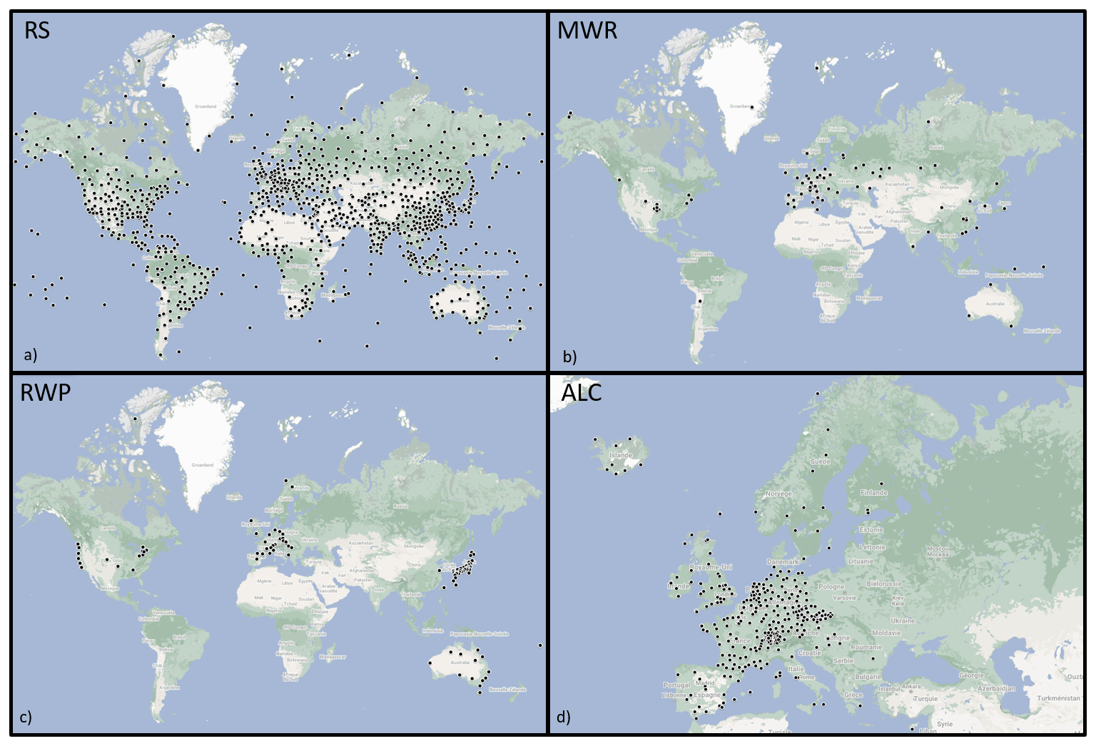
Figure 3 Selected operational networks of profiling stations (status December 2021): (a) global distribution of radiosonde stations (RS, WMO: https://oscar.wmo.int/surface, last access: 23 December 2022), (b) global distribution of microwave radiometers (MWRs, MWRnet: http://cetemps.aquila.infn.it/mwrnet/, MTP-5: http://mtp5.ru/, last access: 23 December 2022, RPG: https://www.radiometer-physics.de, last access: 23 December 2022), (c) global distribution of radar wind profilers (RWP, JMA: https://www.jma.go.jp/jma/en/Activities/windpro/windpro.html#wprsite, last access: 23 December 2022, NOAA: https://psl.noaa.gov/data/obs/datadisplay/, E-PROFILE: https://e-profile.eu/#/wp_profile, last access: 23 December 2022), and (d) European distribution of automatic lidars and ceilometers (ALCs) (E-PROFILE: https://e-profile.eu/#/cm_profile, last access: 23 December 2022). Note that this is by no means a complete representation of all profiling instruments being operated. Additional networks do exist but metadata, such as station locations, are not always easily accessible. Background map © Google Maps 2022.

While radiosonde stations have been organised in coordinated networks for decades, collaborative measurement networks of RWPs, DWLs, MWRs, and ALCs are now also emerging (Fig. 3) because off-the-shelf commercial instruments can now be deployed for unattended, continuous operations, providing atmospheric profile observations in nearly all weather conditions (Sect. 2.2). DIAL and Raman lidars are mostly organised in research networks, such as ACTRIS/EARLINET (https://www.earlinet.org, last access: 23 December 2022) (Pappalardo et al., 2014), NDAAC (https://www.ndsc.ncep.noaa.gov/, last access: 23 December 2022), or PollyNet (Baars et al., 2016), gathering observations of the full troposphere and even lower stratosphere. However, as these sensors are less autonomous compared to MWRs, RWPs, DWLs, or ALCs, spatial coverage tends to be lower for these networks. Other ground-based remote-sensing profiling technologies (e.g. sodar) are to date operated less continuously and at fewer stations for the reasons outlined above (Sect. 2.2).

Worldwide there are ∼ 1300 radiosonde launch sites (Fig. 3a; WMO, 2017), with ∼ 800 stations making observations at least once but mostly twice daily. A subset of upper-air stations (∼ 170) comprises the Global Climate Observing System (GCOS) Upper-Air Network (GUAN; WMO, 2014). The GUAN monitoring centre is hosted at the European Centre for Medium-range Weather Forecasts (ECMWF). Analysis of GUAN data is optimised by the US National Oceanic and Atmospheric Administration (NOAA) National Climatic Data Center (NCDC). NOAA/NCDC archives all GUAN data and makes them available through the Integrated Global Radiosonde Archive (https://www.ncdc.noaa.gov/data-access/weather-balloon/integrated-global-radiosonde-archive, last access: 23 December 2022; IGRA). A subset of GUAN has been selected to establish the GCOS Reference Upper-Air Network (GRUAN; WMO, 2013), providing radiosonde data from reference-quality stations with traceable uncertainty estimates (Bodeker et al., 2016). Higher vertical-resolution radiosonde data, but spatially and temporally more limited, are provided by the Stratospheric–tropospheric Processes And their Role in Climate data centre (http://www.sparc-climate.org/, last access: 23 December 2022; SPARC) through US high vertical-resolution radiosonde data (http://www.sparc-climate.org/data-center/data-access/us-radiosonde/, last access: 23 December 2022; HVRRD).

For both MWR and DWL, networking at a national and international level is still in its infancy (Hirsikko et al., 2014; Thobois et al., 2018), meaning data from these systems could be exploited more effectively in the future. The US ARM programme (http://www.arm.gov/capabilities/instruments/mwrp, last access: 23 December 2022) runs a network of several MWRs (Cadeddu et al., 2013) and also IRSs, though still at a limited number of stations. A first attempt at MWR network operation in Europe was the LUAMI (Lindenberg Upper-Air Method Intercomparison) campaign funded by the German Meteorological Service (DWD) to demonstrate the capabilities of MWR profiler systems for use in operational meteorology. A test network of eight MWR profilers supplied quality-checked data in near-real time to a network hub (Güldner, 2013, and references therein). Several European COST (Cooperation in Science and Technology; https://www.cost.eu/, last access: 23 December 2022) actions taking place over the last 15 years have worked towards the establishment of an international network of MWRs: MWRnet (http://cetemps.aquila.infn.it/mwrnet/, last access: 23 December 2022) is a bottom–up network of users, currently grouping more than 100 MWRs of different types worldwide (Fig. 3b), with 25 profilers located in Europe. MWRnet activities demonstrate the maturity of these sensors for network deployment (Illingworth et al., 2019) and the potential of MWR observations for data assimilation (Caumont et al., 2016). As a consequence, the European national meteorological services network (EUMETNET) accepted the business case for a European MWR network as part of the Composite Observing System (EUCOS) service E-PROFILE (https://e-profile.eu/, last access: 23 December 2022), which is being implemented until 2023 (Rüfenacht et al., 2021).

National RWP networks are operated worldwide (Fig. 3c) utilising various frequencies, i.e. in Australia (14 systems), China (128; Liu et al., 2020), Japan (33; JMA; https://www.jma.go.jp/jma/en/Activities/windpro/windpro.html, last access: 23 December 2022), Canada (7), the United States (9; NOAA; https://psl.noaa.gov/data/obs/datadisplay/, last access: 23 December 2022), and several European countries (32). EUMETNET E-PROFILE coordinates the RWP network operations in Europe, Canada, and Australia. However, many RWPs are not yet integrated into such coordinated networks but are rather operated individually by national hydrological and meteorological services (NHMS), airports, private companies, or research institutions (Ruffieux, 2014).

In Europe, many of the DWLs dedicated to meteorological applications are located at stations that also serve the Aerosol, Cloud and Trace gases Research Infrastructure (https://www.actris.eu/, last access: 23 December 2022; ACTRIS). The US ARM programme operates a network of several DWLs alongside their MWRs and cloud radars (Mather and Voyles, 2013). Operational DWLs are incorporated into the urban meteorological observation system (UMS-Seoul) designed and installed in Seoul, South Korea (Park et al., 2017), and the 3DREAMS network in Hong Kong, China (Yim, 2020), and DWLs are a major component of the New York State Mesonet (https://www2.nysmesonet.org/, last access: 23 December 2022) (Thobois et al., 2018; Brotzge et al., 2020; Shrestha et al., 2021). There is now a significant number of DWLs deployed in commercial networks for wind energy applications mostly dedicated to observing winds at turbine level (around 50–150 m altitude) rather than the full extent of the ABL, and the data may be commercially sensitive.

ALCs are the most widely used instruments in ground-based profile remote-sensing networks. There are several network initiatives coordinating ALC measurements globally, such as the NASA-led Micro-Pulse Lidar Network (https://mplnet.gsfc.nasa.gov/, last access: 23 December 2022) (MPLnet; Welton et al., 2018), the US Environmental Protection Agency (EPA) network for Photochemical Assessment Monitoring Stations (https://www.epa.gov/amtic/photochemical-assessment-monitoring-stations-pams#sites, last access: 23 December 2022) (PAMS; Caicedo et al., 2020), or the Asian Dust and aerosol lidar observation network (ADnet; Shimizu et al., 2016). With more than 370 units (status 2021) transmitting data in near-real time (Fig. 3), EUMETNET E-PROFILE combines the majority of ALC networks established across Europe (Fig. 3d). E-PROFILE ALC data partly coincide with operations of ACTRIS and the European research infrastructure Integrated Carbon Observing System (https://www.icos-cp.eu/, last access: 23 December 2022; ICOS). The latter is increasingly monitoring ABL sub-layer heights for the support of greenhouse gas assessments. ACTRIS has two topical centres (Center for Aerosol Remote Sensing – CARS; Center for Cloud Remote Sensing – CCRES) that are developing services to enhance the quality of ALC measurements. Both ACTRIS and ICOS are currently developing strategies for ABL monitoring in urban settings.

3 ABL height retrievals

Layer boundaries both within and at the top of the ABL (Sect. 1) constitute zones of transition between air of different characteristics. The various physical quantities (Sect. 2.1) derived from profile measurements (Sect. 2.2) each capture some aspects of the ABL development determining these layer heights (Fig. 2). The most common methods developed to retrieve the ABL sub-layer heights from profiles of temperature and humidity (Sect. 3.1), wind and turbulence (Sect. 3.2), or aerosol characteristics (Sect. 3.3) are outlined in this section. Certain approaches (such as the bulk Richardson method described here in Sect. 3.1) in fact exploit a combination of atmospheric variables from different categories. While some measurement systems capture multiple variables simultaneously (e.g. radiosondes), the synergy between measurements from different ground-based remote-sensing profilers (e.g. combining the temperature profile from MWR and wind profile from DWL) is also a promising approach as it allows multi-variable parameters to be calculated.

Limitations and uncertainties are discussed and where possible linked to the characteristics of the sensors used for data collection. Two prominent effects reducing the capability of many active ground-based remote-sensing instruments are (a) a potential blind zone that reduces the capability of observing shallow layers in the near range and (b) insufficient signal strength at higher altitudes. Profilers with a certain blind zone (many lidars or radar wind profilers) do not provide information in the first range gates near the sensor which means, when the signal is sent upwards (e.g. DWL vertical stare or high elevation angles), the first reliable measurement level may be located above a shallow MBLH. In such a case, the derived heights should be interpreted as an “upper limit” of the true MBLH. Similarly, observations obtained under low-SNR conditions (e.g. due to low aerosol load) may not capture the full extent of the ABL (Liu and Liang, 2010) in which case derived layer heights should be considered a lower limit (Bonin et al., 2018; Krishnamurthy et al., 2021).

It is generally challenging to objectively quantify the performance of a method used for layer height detection, mainly because there is no absolute reference for ABL heights against which the derived product could be verified. Instead, evaluation is usually based on intercomparisons, both between methods using the same quantity and between results obtained from different atmospheric variables. During interpretation it is hence key to consider that discrepancies not only reflect the errors in the respective height retrieval methods and the uncertainties in the atmospheric profiles analysed but may further be affected by a series of methodological aspects.

• A potential mismatch can be introduced by the representation of the analysed profile linked to data acquisition or processing (e.g. profile vertical and temporal resolution, averaging, horizontal displacement of the sensor).

• Atmospheric processes portrayed by the observations may differ (e.g. when comparing thermodynamic layer estimates to aerosol-based layer estimates).

• All layer heights in reality relate to a transition zone between two atmospheric layers, so that the specific signature in the atmospheric profile associated with the respective layer height is relevant (e.g. is CBLH located at the bottom, middle, or top of the EZ; Helmis et al., 2012).

Due to the lack of a better alternative, thermodynamic layer heights (Sect. 3.1) derived from radiosonde profiles (Sect. 2.2.1) are most commonly used as a reference (Seibert et al., 2000). However, comparing balloon ascents and ground-based remote-sensing data can be prone to some systematic discrepancies connected to horizontal and temporal variations in ABL dynamics.

• The horizontal drift of the balloon during the ascent means vertical profiles derived from radiosondes may be influenced by spatial variations in ABL dynamics and do not necessarily represent the ABL structure just above the launch site. This impacts the comparison especially where ABL dynamics respond to surface heterogeneities (e.g. Tang et al., 2016; Peng et al., 2017). But the synoptic flow also plays a role given radiosonde balloons are drawn into regions of convergence so that their profiles are more likely to trace convective activities (Schween et al., 2014).

• Spatial displacement between balloon ascents and the ground-based profile can be further altered if the remote-sensing instrument is operating on a moving platform (e.g. ship-based observations; Tucker et al., 2009).

• At the EZ, convective plumes can cause variations in ABLH of the order of several hundred metres (∼ 150–250 m; Hennemuth and Lammert, 2006; Granados-Muñoz et al., 2012) within a few minutes. While some ground-based profiling sensors operate at very high resolution and can hence capture such temporal variations, the radiosondes only monitor the layer boundary at one given instance.

• The agreement between layer heights detected by methods based on different atmospheric quantities varies with atmospheric conditions (such as stability and cloud dynamics; Sect. 4.4). As these usually change through the course of a day, the timing of radiosonde ascents relative to the diurnal cycle of the ABL dynamics can affect the comparison statistics.

• Standard sounding data (i.e. radiosonde profiles reduced to significant pressure levels; Sect. 2.2.1) yield higher ABLH than data at high vertical resolution, which can introduce structural uncertainties of a few hundred metres in long-term statistics.

• Systematic performance errors in the radiosonde humidity sensors (Sect. 2.2.1) lead to reduced accuracy of humidity-based detection methods (Sect. 3.1) in the presence of clouds.

All these aspects should be considered when interpreting limitations of and uncertainties in the various methods. In general, uncertainties in layer height detection vary with time of day and differ between the layer targeted. Uncertainty increases when multiple ABL sub-layers are present given that not only the detection of a layer boundary needs to be accomplished but rather a second step, the so-called layer attribution, is required. Particularly at times with significant temporal variations in ABL dynamics (e.g. morning growth and evening decay of the CBL, formation of a low-level jet, advection of air masses, formation of clouds or fog), multiple layer boundaries need to be interpreted with care.

Beyrich and Leps (2012) developed a scheme that utilises the agreement between different methods (in their case thermodynamic and wind-based detection applied to radiosonde profiles) to quantify the uncertainty in the layer heights at a given moment and assign quality flags accordingly. This is a promising approach that could be further extended where data from multiple systems are available simultaneously so that a range of detection methods based on different atmospheric variables can be applied in synergy.

3.1 Methods based on temperature and humidity

Detection methods for ABL heights based on temperature and/or humidity profiles rely on thermodynamic effects. They allow for the identification of daytime and nighttime layer heights, namely CBLH, SBIH, SBLH, and RLH (Sect. 1; Seibert et al., 2000; Seidel et al., 2010, 2012, and references therein). While some methods are directly applied to the profiles of air temperature, others utilise the potential temperature that considers atmospheric stability or the virtual potential temperature which accounts for atmospheric humidity effects in addition (Fig. 2). Computation of θ (θ_v) requires atmospheric pressure (and humidity), which are at times obtained from external data sources (e.g. other sensors, reanalysis). Some methods directly explore profiles of relative humidity or specific humidity (Beyrich and Leps, 2012). Alternatively to air or potential temperature, the brightness temperature observed by radiometer profilers (Sect. 2.2.2) can be used as input for layer height retrievals, as this physical quantity holds information on both temperature and humidity (similarly to the virtual potential temperature).

Temperature and humidity methods can be applied to profile data from in situ measurements (Sect. 2.2.1), radiometers, DIALs, or Raman lidars (Sect. 2.2.2) but are also very commonly implemented in numerical modelling when ABL heights are diagnosed from the model fields (e.g. Cohen et al., 2015).

3.1.1 Methods

The two most commonly applied temperature-based approaches for the detection of CBLH are the parcel method (Holzworth, 1964) and the bulk Richardson method (Hanna, 1969; Vogelezang and Holtslag, 1996; Zilitinkevich and Baklanov, 2002). The parcel method defines CBLH as the height to which an air parcel with ambient surface air temperature can rise adiabatically from the ground by convection and is obtained by following the dry adiabat from the surface up to its intersection with the temperature profile. While the parcel method is only applicable under unstable atmospheric conditions, the bulk Richardson method takes into account the implications of wind shear contribution to turbulence generation and is hence applicable in all stability regimes. The bulk Richardson number Ri_b represents the ratio of turbulence induced by thermal buoyancy and wind shear, and profiles of both temperature and horizontal wind are required to calculate Ri_b. It is essentially a synergy approach that combines thermodynamic and dynamic effects and could as well be grouped into dynamic retrieval methods (Sect. 3.2). Both CBLH and SBLH can be determined as the altitude where Ri_b exceeds a critical threshold. Typical values of this threshold are around 0.10–0.40 (Sørensen et al., 1996) or 0.25–0.50 (Seibert et al., 2000) with the value 0.25 used to estimate layer heights provided in the ERA-Interim reanalysis data (von Engeln and Teixeira, 2013). The exact threshold value has a relatively modest impact on the layer detection accuracy as long as a value < 0.5 is chosen (Seidel et al., 2012; Guo et al., 2016; Beyrich and Leps, 2012; Cimini et al., 2013). As the bulk Richardson method and the parcel method are identical if the threshold value is set to 0, layer estimates from the former are greater by definition. This increment was found to be about 20 m on average for the CBLH (Collaud Coen et al., 2014). As moisture lightens the air and allows it to rise convectively to greater altitudes, using θ_v instead of θ (Sect. 2.1) in both methods results in slightly greater layer heights (by 3 %–8 %; Collaud Coen et al., 2014).

Both the parcel and bulk Richardson method highly depend on the accuracy of the ambient air temperature at the surface. A temperature excess corresponding to the strength of convective thermals can be added to θ_v at the surface under unstable conditions (Holtslag and Nieuwstadt, 1986; Seibert et al., 2000). This excess temperature is usually applied when the surface air temperature is measured at a height exceeding the standard 2 m, as, for example, in radiosoundings or NWP model data (Stohl et al., 2005).

In addition to the commonly used parcel and bulk Richardson methods, several other thermodynamic methods are available to detect heights of ABL sub-layers, including the following.

• SBIH and SBLH under stable conditions:

  • As a clear indicator of a stable boundary layer, SBIH is diagnosed from air temperature profiles (Bradley et al., 1993; Seidel et al., 2010).

  • At the transition between the SBL and the neutral residual layer, SBLH is marked by a vertical gradient of θ equal to 0 that corresponds to the theoretical lapse rate (Collaud Coen et al., 2014) or is equal to a critical lapse rate determined by the maximum variance of the gradient (Min et al., 2020).

  • Liu and Liang (2010) refine SBLH detection by choosing the first height above ground that either shows a minimum in the potential temperature gradient or a local maximum in horizontal wind speed if an LLJ is present. The method uses surface classification (land, ocean, ice) to determine critical thresholds.

  It should be noted that the accuracy of SBLH (and to some extent SBIH) detection highly depends on the vertical resolution of the analysed temperature profile. In contrast to the parcel method or the Ri_b method, no vertical interpolation or smoothing of the profile data can be performed.

• CBLH under unstable conditions:

  • The Heffter method determines CBLH as the minimum height, where the vertical gradient of θ exceeds 0.005 K m⁻¹ while θ changes by more than 2 K across the inversion layer (Heffter, 1980).

  • The minimum height where θ reaches a certain increment compared to its ABL minimum can mark the CBLH (Nielsen-Gammon et al., 2008).

  • The maximum negative vertical gradient of refractivity (Sect. 2.1) or humidity was found to mark the CBLH (Seidel et al., 2010).

  • Schmid and Niyogi (2012) improve the detection of CBLH by allocating heights where a change in the vertical θ_v gradient coincides with a dew point temperature inversion.

• MBLH independent of atmospheric stability:

  • To derive the MBLH from temperature profiles, both the base of an elevated temperature inversion (Seidel et al., 2010) and the height of the maximum positive θ gradient (Stull, 1988; Seidel et al., 2010) have been applied. As vertical mixing can already be reduced for a certain region below a positive vertical gradient in air temperature, the latter criterion can be a more accurate indicator of MBLH. However, the profile data of atmospheric pressure required to calculate θ may not always be available.

  • Cimini et al. (2013) apply a multivariate statistical regression method trained with real observations to derive MBLH directly from T_b. This method exploits all the information in the MWR observations and is independent of uncorrelated retrieval errors in the temperature and humidity profiles (Sect. 2.2.2) as both systematic and random errors are inherently accounted for.

  • To ensure continuous layer detection, different temperature-based methods can be combined depending on atmospheric stability as the most applicable method may vary during the course of the day and between land cover types. The most common method synergy is probably the combination of the parcel method (CBLH) and the SBIH at night.

Some disagreement between temperature- and humidity-based methods stems from the presence of clouds, which create a complex vertical ABL structure (Sect. 4.6). While humidity-based methods tend to respond to the layer boundary at the cloud top (large negative humidity gradient), the maximum gradient of θ usually occurs in the middle of the EZ above the cloud. To overcome this issue, ABLH can be assigned to the level where all of the above variables exhibit pronounced variations simultaneously, rather than looking for the strongest change in one specific profile variable only.

3.1.2 Capabilities and limitations

Long-term, multi-site comparisons reveal some systematic differences between the various temperature- and humidity-based methods (e.g. Seidel et al., 2010; Beyrich and Leps, 2012). The Heffter method often overestimates MBLH, and the definition of thresholds was found challenging (see discussion in  Caicedo et al., 2020, and references therein). Sinclair et al. (2022) find that agreement and sign of systematic biases depend on atmospheric stability. The T_b regression method (Cimini et al., 2013) provides height estimates that are mostly consistent with the bulk Richardson approach. Methods based on finding extreme vertical gradients are in better agreement with each other than those based on locating elevated temperature inversions (Seidel et al., 2010).

It is generally concluded that uncertainties in layer detection are closely linked to uncertainties in the atmospheric profiles analysed (e.g. errors in surface wind speed, vertical interpolation and vertical resolution; Seidel et al., 2012). Given that such errors are much more pronounced (10 %–80 %) for low layer heights (< 1–2 km), relative uncertainties in the layer detection can be large (> 50 %) for shallow layers but usually remain below 20 % for layer heights > 1 km (Seidel et al., 2012; Aryee et al., 2020; Guo et al., 2016). Uncertainties are usually greatest during the evening decay (Sect. 4.4) of the CBL as this is a time of significant nonstationarity. Methods agree better when applied to radiosonde profiles at midday compared to midnight conditions (Beyrich and Leps, 2012), which further highlights the fact that the CBLH layer boundary is often well-defined, while the detection of SBLH is more ambiguous.

Both the parcel method and the bulk Richardson method are sensitive to surface-level data (Sect. 3.1.1). For example, a change in surface temperature by ±0.5 K leads to uncertainties of the order of ±50–150 m for the maximum CBLH in the early afternoon at a midlatitude continental site (Collaud Coen et al., 2014). Careful quality control of the measurements is hence required to ensure physically reasonable coupling of the surface air temperature value to the first values of the temperature profile (Beyrich and Leps, 2012). Horizontal and/or vertical separation between the site of the surface measurements and the radiosonde launch site can cause artificially large vertical gradients in the combined temperature profile, which may result in significant average differences in the derived ABLH of up to several hundred metres (Seidel et al., 2010). In such a case, it is preferable to initialise the layer detection with values at the first reported upper-air level instead of surface observations.

From an analysis using MWR data, Collaud Coen et al. (2014) found the parcel method to be more robust and hence better suited for automatic real-time detection of the CBLH compared to the bulk Richardson method because the latter requires more input data. In addition to the temperature (and pressure) data, wind profile observations are needed, which introduces additional measurement uncertainties and missing values from a second system. Such issues are slightly reduced when the methods are applied, for example, to radiosonde data, as here both wind and temperature are gathered by the same measurement system. Due to the simplicity of the parcel method, it is more likely to capture shallow layer heights. Seidel et al. (2010) conclude that diurnal and seasonal variations based on this method generally tend to have a greater amplitude and can be considered more consistent than those derived from other approaches. This is in agreement with the analysis by Collaud Coen et al. (2014).

The method using T_b regression analysis (Cimini et al., 2013) relies on “independent training data”. Given there is no absolute reference when it comes to ABL heights, the choice of training data and potential systematic differences in the physical representation of ABL dynamics by the observed quantity analysed and the respective detection approach can affect the performance of this method. Still, even when trained with aerosol-derived layer estimates (Sect. 3.3), the T_b regression method shows better agreement with layer estimates from the bulk Richardson method applied to radiosonde profiles compared to the parcel method and θ_v-gradient method applied directly to temperature and humidity data from the MWR.

The presence of clouds increases uncertainty in CBLH retrievals for all methods (Sect. 4.6), so that temperature-based methods applied to radiosondes and MWR profile data show better agreement during clear-sky days (Cimini et al., 2013). When the parcel method is applied to temperature profile data obtained from radiosondes and MWR, the latter tend to significantly underestimate the MBLH (Cimini et al., 2013). Up to now, no quantitative, comparison analysis has been performed regarding MBLH estimates from different MWR types, although there have been field campaigns wherein multiple commercial MWRs were operated side by side, such as the Joint CALibration experiment (JCAL; Pospichal et al., 2016) or the recent Field Experiment on Submesoscale Spatio-Temporal Variability in Lindenberg (https://fesstval.de/, last access: 11 January 2023; FESSTVaL).

3.2 Methods based on wind or turbulence

Methods exploiting wind profile observations to detect ABL heights can generally be grouped into those using components of the mean wind and those based on turbulence indicators. The objective of these methods is to identify the height of the turbulent layer connected to the surface. The mixing is either caused by buoyancy-driven turbulence or shear-driven turbulence, or a combination of the two. Intermittent turbulence in the residual layer can affect the performance of layer detection algorithms (Pichugina and Banta, 2010), but wind and turbulence methods are usually not applied to detect RLH.

3.2.1 Methods

Using mean wind profiles (Fig. 2), the most commonly applied layer detection approach is the bulk Richardson method, which requires temperature profile data in addition (see Sect. 3.1). Looking at the relation between thermally induced buoyancy and shear-induced turbulence, this synergy method is applicable under all stability conditions (i.e. for detection of both SBLH and CBLH). Alternatively, SBLH can be identified as the height of a local maximum in horizontal wind speed or a local minimum in vertical wind speed or wind shear (Balsley et al., 2006; Banta et al., 2006; Pichugina and Banta, 2010; Lemone et al., 2014). Johansson and Bergström (2005) find that significant changes in the mean ascent rate of radiosonde balloons indicate the transition from turbulent to non-turbulent regimes, thereby exploiting a mean quantity to diagnose turbulence indicators indirectly (Lemone et al., 2014).

Due to advances in high-resolution ground-based profiling, direct measures of atmospheric turbulence can be determined quantitatively with increasing accuracy (Sect. 2.2.3). Turbulence can be diagnosed from the refractive index structure parameter (Sect. 2.1) observed by sodar and RWP (Sect. 2.2.3). The peak in the vertical profile of the refractive index structure parameter caused by small-scale buoyancy fluctuations across the entrainment zone has been found to coincide with the MBLH (White, 1993; Angevine et al., 1994; Wilczak et al., 1997). Given that these fluctuations are associated with relatively high SNR in sodar and RWP observations, some methods assign CBLH to a local peak in RWP SNR (B. Liu et al., 2019; Collaud Coen et al., 2014). RLH can also be detected by analysing profiles of $C_n^{\mathrm{2}}$ but only for specific (mostly cloud-free) weather conditions. ABLH is diagnosed from spaceborne GNSS-RO observations as the strongest negative gradient in refractivity (Ao et al., 2012; Chan and Wood, 2013) that is associated with the strong moisture and temperature gradients usually present at the top of the ABL (Xie et al., 2012).

Estimates of atmospheric turbulence can also be obtained from temporal and/or spatial fluctuations in high-resolution wind profiling data. The most commonly exploited turbulence variables derived from high-frequency wind components are the variance of vertical velocity, variance of horizontal velocity, turbulent kinetic energy, and the eddy dissipation rate (Sect. 2.1). To ensure layer detection relies on the measurement of turbulence intensity, it is important to remove non-turbulent fluctuations from the wind field components (Bonin et al., 2018). Applying a high-pass filter was found to be a simple but effective means to sufficiently reduce the influence of submesoscale motions, drainage flows, and gravity waves (Bonin et al., 2017, 2018), with frequencies on the order of minutes to tens of minutes (Finnigan et al., 1984). Berg et al. (2017) chose to detect layer heights based on the normalised vertical velocity variance to reduce the impact of coherent vertical motions above the ABL.

During convective atmospheric conditions, the vertical velocity variance from vertically pointing profile observations is the most direct measure of the instantaneous mixing within the CBL. The CBLH is commonly assigned to the height above ground where the vertical velocity variance (Fig. 2) falls below a set threshold, with both absolute (0.04–0.16 m² s⁻²; Tucker et al., 2009; de Arruda Moreira et al., 2018; Barlow et al., 2011; Huang et al., 2017; Vakkari et al., 2015; Theeuwes et al., 2019) and relative values (e.g. 10 % of profile maximum; Barlow et al., 2011) implemented successfully. Given the gradual decay of turbulence in the afternoon and evening CBL, Schween et al. (2014) find CBLH detection to be particularly sensitive to the threshold value during this period. The choice of threshold value can depend on the ABL structure (Tucker et al., 2009; Huang et al., 2017) and the scanning-strategy-dependent noise levels (Bonin et al., 2018). When shear-driven turbulence dominates, horizontal velocity variance becomes a better indicator of the layer boundaries. The vertical profile of horizontal velocity variance depends on atmospheric stability, with a near-surface peak under slightly stable conditions, a rather constant vertical distribution under medium stable conditions, and a maximum aloft near the core of the LLJ under strongly stable conditions (Banta et al., 2006). Tucker et al. (2009) use the same threshold values as for the vertical velocity variance to determine shallow layer heights from horizontal velocity variance.

Lemone et al. (2014) find a relative value of 5 % of the profile maximum TKE most suitable for the detection of SBLH, while LeMone et al. (2013) apply fixed values (0.101 and 0.200 m² s⁻²) to determine CBLH from model data. Vakkari et al. (2015) assign CBLH to the height where the eddy dissipation rate falls below 10⁻⁴ m² s⁻³, while Frehlich et al. (2006) examine the strongest negative gradient of this quantity. For specific scan patterns, the variance of radial velocity (i.e. the native variable obtained form Doppler wind lidar measurements) is directly related to TKE (Sect. 2.2.3) and is hence also exploited for layer detection. Pichugina and Banta (2010) determine the SBLH as the height of the first significant local minimum in the vertical profile of the radial velocity variance obtained from vertical-slice scans.

Under well-mixed, convective conditions, i.e. when CBLH coincides with ABLH, turbulence-based detection methods can be supported by applying SNR requirements (de Moreira et al., 2015; Pearson et al., 2010; Singh et al., 2016). Lothon et al. (2006) evaluate the total velocity variance from DWL observations for layer detection, which inherently includes the SNR information as the recorded signal responds to both atmospheric variations and instrument-related noise (Tucker et al., 2009).

To cover the full range of MBLH at a given measurement location, wind or turbulence measurements from multiple data sources can be combined (e.g. sodar and RWP; Beyrich and Görsdorf, 1995; Beyrich, 1997; Angevine et al., 2003). The great advantage of scanning DWL systems is that a series of wind and turbulence variables can be obtained within a rather short time interval by a single sensor (Sect. 2.2.3). For example, vertical stare measurements can be alternated with range–height indicator (RHI) scans (Tucker et al., 2009) to monitor convection or plan position indicator (PPI) scans at low elevation angles (Vakkari et al., 2015) to capture shallow layers. To facilitate the composition of layer information from various atmospheric variables (mean wind fields, different turbulence indicators, SNR), fuzzy logic algorithms (Bianco and Wilczak, 2002; Bianco et al., 2008; Allabakash et al., 2017) or machine learning (Krishnamurthy et al., 2021) are increasingly implemented. Recent advanced approaches (Bonin et al., 2018; Krishnamurthy et al., 2021) combine a diverse set of atmospheric variables, which enables reliable layer detection under nearly all atmospheric conditions. To enhance agreement with aerosol-derived layer heights (Sect. 3.3), Bonin et al. (2018) give less weight to the vertical velocity variance during layer height retrieval, thereby moving the focus towards those indicators that portray the resulting “mixed conditions” instead of the mixing process itself. Where the ABL responds to significant surface heterogeneities (Banks et al., 2015; Haid et al., 2020; Vakkari et al., 2015), a site-specific design of DWL scanning strategies is recommended to best capture the variability in MBLH.

3.2.2 Capabilities and limitations

The altitude range of the atmospheric profile measurements and the accuracy of wind and turbulence data from ground-based remote-sensing systems depends on instrument capabilities and measurement setup (Sect. 2.2.3). The ability to detect shallow layers generally depends on how large the blind zone of the sensor is, while observing that the full depth of deeper convective conditions is dependent on SNR. Turbulence-based MBLH estimation is particularly applicable in daytime convective conditions (Bianco et al., 2008; Collaud Coen et al., 2014). Decaying turbulence in the residual layer can be a source of added uncertainty (Lemone et al., 2014).

Rainfall can be a significant source of uncertainty for automatic layer detection from profiles of wind and turbulence. It is possible to diagnose rainfall from the vertical velocity profile based on the terminal fall speed of the rain drops (e.g. using column-averaged vertical velocity $<-\mathrm{1}$ m s⁻¹; Bonin et al., 2018), but such filters will not detect precipitation conditions with lower fall speeds (such as drizzle or snow) and can miss precipitation that evaporates before reaching the surface (virga).

3.3 Methods based on attenuated backscatter

The distribution of aerosols and moisture usually results from a complex combination of processes, including emission, formation, accumulation, deposition, transport (advection), and also mixing. Profiles of attenuated backscatter (Sect. 2.1) hence trace some aspects of the recent history of ABL dynamics. Layer boundaries can be detected if aerosol properties differ between the atmospheric layers examined. The most pronounced layer edge is usually the ABLH because aerosol concentrations and humidity tend to be significantly higher in the ABL than in the FT (Fig. 2). But within the ABL, mixing dynamics can also lead to contrasting signatures between different layers. During the night and in the early morning, the lowest layer is considered the MBLH (SBLH under stable conditions), while the layer above defines RLH (Sect. 1). During unstable conditions, the aerosol-based MBLH forms partly in response to recent mixing processes. Vertical and temporal changes in aerosol characteristics recorded at high resolution allow EZ characteristics to be examined. Decoupled, elevated aerosol layers above the ABL can be identified if they possess distinct aerosol characteristics. Lidars that capture additional information (such as depolarisation and colour ratio; Sect. 2.1) can provide valuable insights that allow boundary layer aerosols to be better distinguished from lofted layers (e.g. Bravo-Aranda et al., 2017).

The physical quantity of attenuated backscatter is most commonly observed by ALCs or aerosol research lidars (Sect. 2.2.4) but can also be derived from DWLs (Sect. 2.2.3). Layer heights derived from different systems can be combined to overcome instrument-related limitations; e.g. results from more powerful lidars can be combined with those from ALC observations (e.g. Wang et al., 2020). As the majority of layer detection algorithms does not rely on absolute values of attenuated backscatter but rather assesses relative variations in this quantity in time and height, the range-corrected signal is often used as an alternative input. Also, profiles of SNR (from, e.g., ALC, DWL, or RWP; Compton et al., 2013; Molod et al., 2015, 2019) can be used as input under the assumption that this variable is directly related to the distribution of scatterers in the atmosphere. While the discussion here focuses on ground-based profilers, it should be noted that aerosol-based techniques can also be used for the analysis of airborne lidar profiles (e.g. Scarino et al., 2014), satellite data (CALIOP; Zhang et al., 2016), or output from numerical simulations.

3.3.1 Methods

Aerosol-based retrievals of ABL heights detect layer boundaries based on regions of significant vertical (and at times temporal) change in attenuated backscatter. Where multiple layers are present within the ABL, the role of the respective layers needs to be examined carefully. Hence, two steps are required to determine the ABL heights from aerosol backscatter observations: (1) detection of layer boundaries within and at the top of the ABL and (2) layer attribution to distinguish between simultaneous layers (e.g. MBLH and RLH). Methods that predominantly address the task of layer detection are here considered first-generation aerosol-based retrievals, while those with a special focus on the more challenging aspect of layer attribution are grouped into second-generation aerosol-based retrievals.

To detect heights (or regions) of potential layer boundaries from attenuated backscatter profiles, a range of indicators has proven useful (see reviews by, for example, Emeis et al., 2008; Dang et al., 2019). These include negative vertical gradients and inflection points (e.g. Sicard et al., 2006; Emeis et al., 2008; Münkel, 2007; Schäfer et al., 2004; Lee et al., 2019), 2D edge detection (e.g. Canny, 1986; Parikh and Parikh, 2002; Haeffelin et al., 2012), wavelet covariance transform (WCT; e.g. Cohn and Angevine, 2000; Morille et al., 2007; Baars et al., 2008; de Haij et al., 2006; Gan et al., 2010; Granados-Muñoz et al., 2012; Lewis et al., 2013; Caicedo et al., 2020), the cubic root gradient which takes into account the influence of gravity waves (Yang et al., 2017), and spatio-temporal variance (e.g. Menut et al., 1999; Martucci et al., 2007; Lammert and Bösenberg, 2006; Piironen and Eloranta, 1995; Hooper and Eloranta, 1986). For example, ABLH is derived from CALIPSO satellite observations as the maximum in vertical and horizontal variance (Jordan et al., 2010).

Many layer detection methods show varying reliability at different stages of the diurnal ABL evolution. ABLH is usually marked by the strongest negative gradient in attenuated backscatter. The mixing between moist ABL air and dry FT air across the EZ results in an area of strong spatio-temporal variance (e.g. Menut et al., 1999). But entrainment of RL air into the CBL during morning growth can also cause distinct variance signatures (e.g. Lammert and Bösenberg, 2006). While some methods (such as the wavelet approach) are less affected by noise, the simple method of vertical gradient detection can be advantageous in capturing layers in low ranges (Di Giuseppe et al., 2012).

Several approaches have been developed to accomplish the second task of layer attribution. First-generation retrieval methods apply attribution criteria either to the respective indicator (e.g. strongest negative vertical gradient) and/or simply based on height (e.g. first significant negative gradient above ground) to assign the layer of interest. Second-generation retrieval algorithms again can broadly be grouped into the following categories:

• Methods based on general layer characteristics. These methods group aerosol data along the vertical profile into categories. To differentiate between the ABL with a high aerosol load and the FT with a low aerosol signal, an idealised profile can be fitted to the observations (e.g. Steyn et al., 1999; Eresmaa et al., 2006, 2012; Li et al., 2017; Peng et al., 2017). Recent artificial intelligence (AI) approaches analyse the profile further across the whole layer, including extended Kalman filters (Lange et al., 2013; de Arruda Moreira et al., 2018; Kokkalis et al., 2020), K-means cluster analysis applied to either the attenuated backscatter profile (KABL; Toledo et al., 2014; Rieutord et al., 2021; Min et al., 2020) or layer candidates derived from first-generation methods (ISABL; Min et al., 2020), or a supervised AdaBoost algorithm (ADABL; Rieutord et al., 2021).

• Combination of identification techniques. Given that the various layer detection techniques can be sensitive to slightly different layer boundaries, a combination of indicators can help to distinguish between layers. For example, Martucci et al. (2010a) combine the height of the maximum negative gradient and the height of maximum variance to detect MBLH both during the day and at night together with lofted, decoupled aerosol layers. STRAT-2D (Morille et al., 2007; Haeffelin et al., 2012) uses the variance field to determine which wavelet-detected layer boundary is likely associated with MBLH by analysing the location of the EZ. PathfinderTURB (Poltera et al., 2017) and STRATfinder (using advantages of STRAT+ and pathfinderTURB; Kotthaus et al., 2020) combine gradient and variance field diagnostics before tracing MBLH. COBOLT (Geiß et al., 2017) uses a combination of gradients, variance statistics and WCT, varying with solar angle to identify the MBLH. Applying gradient-boosted regression trees, de Arruda Moreira et al. (2022) combine an MBLH first estimate derived using the gradient method with several meteorological variables to retrieve MBLH values that are comparable to those derived from a microwave radiometer, discriminating between CBLH and SBLH. The profile fit approach is combined with WCT by Sawyer and Li (2013) and with the negative gradient detection in the proprietary Vaisala BLview software (Münkel, 2016). It should be noted that the BLview algorithm provides several layer candidates so that some post-processing is required to select the appropriate MBLH. This has been achieved, for example using the provided quality flags (Geiß et al., 2017), gradient thresholds (Haman et al., 2012), manual screening (Caicedo et al., 2017), or a combination of time-tracking and height criteria (Mues et al., 2017; Lotteraner and Piringer, 2016).

• A priori assumptions based on ancillary observations. Where climatology statistics are available from independent measurements (e.g. radiosondes) limits can be prescribed that may vary by season. For example, in pathfinderTURB and STRATfinder absolute limits for MBLH and morning transition growth rate are specified by the user. Some studies set time-specific coefficients (morning, afternoon, and night) for the WCT (Gan et al., 2011; Caicedo et al., 2020). STRAT+ (based on STRAT-2D; Pal et al., 2013) uses radiosonde profiles and turbulent surface sensible heat flux measurements to derive stability information that aid interpretation of the variance field.

• A priori assumptions from model results. Simple models describing general ABL dynamics or output from NWP models representing varying synoptic conditions have been used to guide layer attribution. For example, Di Giuseppe et al. (2012) use a bulk model (Tennekes, 1973) based on surface sensible heat flux data to define times of morning and evening transition.

• Temporal layer tracking. Temporal consistency is a powerful criterion for layer attribution (Angelini et al., 2009) as it reduces physically unreasonable height fluctuations and growth rates. For example, the temporal-height-tracking method (THT; Martucci et al., 2010a) uses the MBLH estimate at a previous time step to define the search window for the subsequent detection. A similar approach is implemented in COBOLT (Geiß, 2016) and by Wang et al. (2012) or Caicedo et al. (2020). The MIPA algorithm (Vivone et al., 2021) uses morphological and object-based image processing techniques to improve temporal consistency of the detected MBLH. A recent family of algorithms (pathfinder, pathfinderTURB, STRATfinder) applies a graph theory approach to trace the path of MBLH through the day. In CABAM (Kotthaus and Grimmond, 2018a), points of significant negative gradients are connected to layers which are then traced through the day following growth and decay criteria in a dynamic decision tree. The extended Kalman filter applied by Kokkalis et al. (2020) uses information from past profile analysis to inform ABLH detection, which generally improves temporal consistency. Also, the supervised ADABL algorithm (Rieutord et al., 2021) considers temporal consistency.

• Additional lidar profiles. The POLARIS algorithm analyses the depolarisation ratio in connection with the WCT approach (Bravo-Aranda et al., 2017). The MDS method (Liu et al., 2018) determines ABLH by adding information on the particle size by calculating the degree of difference in aerosol characteristics between observations from two adjacent lidar range gates as a combination of aerosol backscatter and the colour ratio. As research lidars and some novel ALCs provide not only attenuated backscatter but also other additional profile information (e.g. depolarisation ratio), promising developments are expected from algorithms that exploit more than one aerosol variable to differentiate between layer characteristics.

While most of these retrieval algorithms output one layer height (usually either MBLH or ABLH), simultaneous identification of several layers is possible provided the layer attribution step does account for it (Kotthaus et al., 2020; Milroy et al., 2012; Caicedo et al., 2020; Toledo et al., 2017). Elevated aerosol layers can be traced in addition to ABL heights. For example, Poltera et al. (2017) detect a continuous aerosol layer above the ABL using pathfinderTURB, while Pandolfi et al. (2013) track a decoupled aerosol layer above the ABL using the THT algorithm and Gan et al. (2010) derive RLH and elevated aerosol layers using the WCT approach.

In the absence of clouds, aerosol-derived ABLH is usually positioned somewhere in the centre of the EZ, where vertical negative gradients and spatio-temporal variance are strongest due to the exchange of aerosols and moisture between the ABL and FT (Menut et al., 1999). Where observations at very high temporal resolution of the order of minutes are available and SNR is sufficient, temporal variations in ABLH permit the estimation of the EZD (e.g. Cohn and Angevine, 2000) and entrainment velocities (Träumner et al., 2011). Martucci et al. (2010a) performed spectral analysis on high-resolution ABLH observations to characterise entrainment processes under different atmospheric stability conditions. Alternatively, the transition zone concept, based on the difference between high attenuated backscatter values in the ABL and low values in the FT (Steyn et al., 1999) can be used to determine the EZD. Statistical concepts capturing temporal, spatial, and small-scale turbulence variations can differ significantly from the transition zone estimates, given the latter is mostly limited to small-scale turbulence effects (Träumner et al., 2011).

3.3.2 Capabilities and limitations

Both the detection and the attribution step of aerosol-based layer retrievals highly depend on the quality of the attenuated backscatter profiles analysed (de Haij et al., 2006; Milroy et al., 2012). MBLH and ABLH retrievals based on attenuated backscatter have seen significant improvements due to recent advances in ALC measurement technology (Illingworth et al., 2019; Cimini et al., 2020) and detailed correction procedures (Hervo et al., 2016; Kotthaus et al., 2016) as both improve data quality and availability. Any combination of high instrument-related noise, low aerosol (and moisture) load, or very deep convection reduces the SNR, which can lead to both underestimation and overestimation of peak ABLH (Kotthaus et al., 2020). Applying an SNR filter can improve layer detection (Poltera et al., 2017; Min et al., 2020); however, care must be taken in pristine environments (Boy et al., 2019) wherein atmospheric scatterers are scarce and the recorded signal may not necessarily exceed instrument and background noise significantly. While SNR limitations mostly lead to uncertainties in the detection of layer boundaries at elevated heights above ground, the detection of shallow layers (nocturnal MBLH and SBLH) can be affected by the incomplete optical overlap and near-range artefacts (Schween et al., 2014; Kotthaus et al., 2020; Caicedo et al., 2020).

In addition to instrument-related uncertainties, discrepancies in layer results arise from the choice of retrieval algorithm. Haeffelin et al. (2012) compared five MBLH detection techniques applied to observations from three different ALCs at two contrasting measurement sites. While layer detection methods (first derivative, WCT, and two-dimensional derivative) often agree, the greatest uncertainty in final products was associated with the step of layer attribution, even when considering simple categories only. Second-generation algorithms (Sect. 3.3.1) hence put a special focus on the interpretation of the ABL sub-layers. Comparing different second-generation methods, it appears that those including criteria on temporal consistency of layer estimates tend to perform slightly better (de Bruine et al., 2017; Knepp et al., 2017).

Agreement between retrieval methods varies with the complexity of the ABL structure. Provided that there is a sufficient SNR, results from different methods and sensors tend to agree best in the afternoon during peak convective activity (Milroy et al., 2012) when the CBL extends over the whole ABL leaving essentially no sub-layers to confuse the algorithms (Toledo et al., 2017). Layer attribution is challenged when several aerosol layers are present simultaneously, such as during the night and in the early morning. If MBL and RL aerosols have similar characteristics, the MBLH may not be characterised by a particularly strong gradient (Granados-Muñoz et al., 2012). The highest uncertainty generally occurs during the evening transition (Geiß et al., 2017) when new aerosol gradients start to form gradually and decaying turbulence may not be traced successfully by backscatter variance methods in the case of homogeneous aerosol distributions (Poltera et al., 2017). In addition to ABL-internal sub-layers, elevated aerosol layers add complexity and hence layer retrieval uncertainty. Any aerosol-based method is challenged when temporal variations in gradients (or variances) are dominated by the advection of aerosols (e.g. due to strong sea breezes or dust transport; Tang et al., 2016; Bravo-Aranda et al., 2017; de Arruda Moreira et al., 2020; Diémoz et al., 2019b; Caicedo et al., 2019). Advances in measurement technology (such as depolarisation information becoming increasingly available; Sect. 2.2.4) and continued algorithm development (including AI methodologies; Rieutord et al., 2021) are expected to further improve layer attribution efforts.

The lidar signal is strongly attenuated by liquid clouds, so that the signal is often completely extinguished at a few hundred metres above the cloud base (depending on the system characteristics; O'Connor et al., 2004) so that profiles of attenuated backscatter yield little information above this height. Where clouds form within the ABL, aerosol-derived layer heights can severely underestimate CBLH (Hennemuth and Lammert, 2006). Advanced detection algorithms hence increasingly take into account the presence of boundary layer clouds (Poltera et al., 2017; Caicedo et al., 2020). Where the cloud-base height variable provided by the ALC is used, it should be noted that this product can show systematic differences between internal algorithms from various manufacturers (Martucci et al., 2010b; Pattantyús-Ábrahám et al., 2017) and even between models from the same brand (L. Liu et al., 2015). Most methods naturally struggle with reliable layer detection and attribution during precipitation or the passage of synoptic fronts (de Bruine et al., 2017; Yang et al., 2017) as the ABL is generally poorly defined during those times when surface–atmosphere interactions play a minor role compared to larger-scale processes.

Some studies assign a quality flag to the derived layer heights based on the magnitude of the attenuated backscatter vertical gradient (e.g. de Haij et al., 2006; Ketterer et al., 2014). For ABLH, such indicators can be suitable given the strong contrasts in aerosol content between the ABL and the FT. However, the strength of the vertical gradient does not necessarily reflect the uncertainty in MBLH detection at night or during morning growth as the contrast is often weaker between the layer coupled to the surface and the RL than between the ABL and the FT. Careful quality control during post-processing (e.g. based on physically reasonable temporal variations in layer heights) can help focus intercomparison or evaluation efforts (Kotthaus et al., 2020; Caicedo et al., 2020).

Aerosol-based retrievals for ABL heights are most commonly evaluated against thermodynamic retrievals (Sect. 3.1) applied to radiosonde profile data (Sect. 2.2.1). When comparing aerosol-derived layers to thermodynamic results, the differences in the underlying physical processes need to be taken into account during interpretation (Hennemuth and Lammert, 2006). Naturally, comparison statistics vary with the retrieval method applied to the radiosonde data (Haman et al., 2012). Compared to thermodynamic estimates, aerosol-derived CBLH can have a negative bias (e.g. de Haij et al., 2006; Bravo-Aranda et al., 2017; de Bruine et al., 2017; Liu and Liang, 2010) as the atmospheric quantities of temperature and aerosol show different EZ characteristics (see discussion in Sect. 4.2). Best agreement between the temperature- and aerosol-based layer height detection is again found in the early afternoon, when the CBL extends over the whole ABL (de Bruine et al., 2017). Given the impact of advection on ABL complexity, agreement between the different approaches can vary with synoptic conditions or local circulations induced by surface cover heterogeneities (Pandolfi et al., 2013; Hennemuth and Lammert, 2006). Liu et al. (2018) find agreement between several aerosol-based ABLH results, and the bulk Richardson method applied to daytime radiosonde profiles clearly improves with increasing atmospheric instability.

Thermodynamic detection of the height of the CI from radiosondes or AMDAR profiles (Sect. 2.2.1) were found to coincide well with aerosol-derived RLH (Martucci et al., 2007; Kotthaus et al., 2020; Milroy et al., 2012). The few studies showing direct SBLH comparisons between aerosol-derived and thermodynamic results generally suggest a good agreement between the layer estimates, with small biases reported in either direction (Pal et al., 2013; Haman et al., 2012; Tang et al., 2016). Still, substantial systematic biases may occur, with aerosol-derived MBLH remaining below SBIH (Marsik et al., 1995). Mismatches are explained by the contrasting physical processes that are being traced, such as when radiative cooling leads to the formation of a surface-based temperature inversion which is not necessarily associated with any contrasts in aerosol characteristics (Milroy et al., 2012).

Due to the lack of suitable reference data and the physical difference between aerosol-based and thermodynamic layer detection, a few studies applied manual or semi-automatic layer detection for the evaluation of aerosol-based retrievals (de Bruine et al., 2017; Poltera et al., 2017; Kotthaus and Grimmond, 2018a). Although manual detection can be a very valuable tool, it is labour-intensive and not necessarily objective (Poltera et al., 2017).

4 Monitoring ABL heights

As ground-based remote-sensing profilers have different capabilities (Sect. 2.2) and algorithm uncertainties depend on a variety of atmospheric characteristics, the performance of the various sub-layer height retrieval methods (Sect. 3) changes throughout the diurnal evolution of the ABL (de Arruda Moreira et al., 2018). The following section summarises the most important strengths and weaknesses of the methods when monitoring the height of the boundary layer at night or during stable conditions (Sect. 4.1), morning growth (Sect. 4.2), peak CBL development (Sect. 4.3), and evening decay (Sect. 4.4). Further, capabilities are discussed that are relevant for the characterisation of the entrainment zone (Sect. 4.5) and the cloud-topped ABL (Sect. 4.6).

The few available synergy applications are highlighted to indicate possible future pathways of ground-based remote-sensing implementation. Where observations from multiple profilers are available simultaneously, analyses suggest that a synergistic interpretation of results from different methods could lead to an enhanced description of the ABL, including the detection of sub-layer heights (Saeed et al., 2016) and the description of the processes shaping the ABL development (Manninen et al., 2018). In addition, combining observations from several sensor systems provides crucial information for the assessment and quantification of layer detection uncertainties (e.g. Cohen et al., 2015) and could be exploited to assign quality flags for the derived layer heights (as has been done for various retrievals from radiosonde profiles by Beyrich and Leps, 2012).

It should be noted that studies directly intercomparing ABL height retrievals based on different atmospheric quantities are still rare, especially those covering extended time periods. Given their impact on layer height uncertainty, measurement setup (such as MWR calibration, DWL focal setting and scan strategy, aerosol lidar optical overlap, amongst others; Sect. 2.2), data processing, and quality control (Sect. 3) should all be carefully evaluated when comparing results from various methods.

4.1 Nocturnal and/or stable boundary layer heights

At night, the MBLH is rather shallow, with stable conditions being more likely. For the detection of shallow layers, a low first measurement level and high vertical resolution of the profile data are beneficial. In situ data obtained on tall towers, on tethered balloons, or using UASs, for example, usually provide very detailed information; however, observations from the airborne platforms tend to lack temporal coverage. For radiosondes launched with automatic systems, measurement uncertainties in the lowest part of the profile can pose challenges for the assessment of very shallow layer heights or near-surface stability conditions.

For ground-based remote-sensing instruments, the near-range capabilities are critical (Sect. 2.2). Layer heights can only be detected if they exceed a potential blind zone of the instrument and they are not obscured by sensor-related uncertainties. MWRs are very suitable for shallow layer height detection given their sensitivity is maximal near the sensor (Sect. 2.2.2). High-power research lidars often do not provide information in the lowest few hundred metres (Sect. 2.2.4), meaning that ALCs can be more suitable for the detection of shallow layers when using aerosol-based methods. Improved monitoring of the lowest few hundred metres of the atmosphere at high vertical resolution can be achieved by operating active remote-sensing profilers at a low elevation angle (e.g. ALC; Poltera et al., 2017). Scanning DWLs (Sect. 2.2.3) can alternate scans at low and high elevation angles, whereby the associated wind and turbulence retrievals have to assume spatial homogeneity of the atmosphere across the sampled volume.

Where both temperature information and wind information are available (e.g. from in situ observations or through instrument synergy), SBLH can be derived from the profile of the bulk Richardson number (Sect. 3.1). While results of this method are particularly sensitive to the first-level air temperature observations, uncertainty may increase in general when combining results obtained from two sensor types (e.g. DWL and MWR). SBLH and SBIH can be determined from features in the temperature profile. In the presence of an LLJ (Sect. 3.2), wind and turbulence profile data not only allow for the retrieval of SBLH but also help interpret its effects on mixing and advection of moisture, heat, and pollutants (Hu et al., 2013; Reitebuch et al., 2000; Bennett et al., 2010). The relation of SBIH to the position of the LLJ changes over time, with SBIH increasing over the course of the night often to exceed the height of the LLJ maximum at some point (Mahrt et al., 1979). In general, discrepancy between temperature-based methods and those analysing vertical wind profiles can be profound during stable conditions (Beyrich and Leps, 2012). Aerosol-based methods can track shallow MBLH if quality observations in the near range are available and careful layer attribution is performed to reduce potential confusion with the RLH.

Some systematic differences in nocturnal MBLH are reported between results from the various methods available (Sect. 3), with discrepancies between layers detected based on the same or different atmospheric quantities at the same order of magnitude. On average, uncertainty in SBLH detection is estimated around 30 %–40 % (Steeneveld et al., 2007). Since turbulence in the SBL is usually not uniform (Beyrich, 1997), the diagnosed layer heights can differ systematically from thermodynamic or aerosol-based methods. While Schween et al. (2014) find turbulence-based nocturnal MBLH exceeds aerosol-based layer heights by about 300 m on average during stormy winters in rural Germany, average nocturnal MBLH differences between turbulence and aerosol-based methods in London, UK, are mostly of the order of their day-to-day variability (Barlow et al., 2011; Kotthaus et al., 2018). More studies are needed to assess the impact of ABL dynamics and atmospheric stability on the relative agreement of the various methods for nocturnal layer height detection.

At night (and in the early morning), the detection and layer attribution of the MBLH (SBLH) can be challenged by the presence of the RL. Layer detection becomes more uncertain if atmospheric characteristics are similar within the MBL and the RL above. As aerosol-based methods are particularly challenged by the presence of an RL, most second-generation algorithms (Sect. 3.3) aim to specifically address this source of error. Further, aerosol characteristics (e.g. size distributions) and intermittent turbulence can cause signatures in attenuated backscatter and turbulence fields, respectively, that may appear as additional layer boundaries within the RL. For the turbulence analysis, layer detection can be improved by distinguishing between surface-driven processes in the MBL and the decoupled mixing above (Sect. 4.7). Temperature-based layer heights (Sect. 3.1) derived from MWR profiles (Sect. 2.2.2) are less likely to mistake elevated layer boundaries for MBLH as these profilers are more reliable in the near range and respond less to RL signatures.

The RL is a remnant of the previous day's CBL (Sect. 1) so that aerosols and moisture remaining in this elevated layer above the MBLH present very suitable atmospheric tracers. While some turbulent exchange between the RL and the FT can be picked up (Fochesatto et al., 2001), the RLH can be tracked most reliably using thermodynamic retrievals (Sect. 3.1) of the CI applied to airborne in situ sensors or by aerosol-based methods (Sect. 3.3) because the contrasts at the ABLH are usually striking. As MWR profiles are generally less sensitive to contrasts near the RLH (Sect. 2.2.2) algorithms are usually not applied to radiometer profiles for the detection of this RLH. Uncertainty in RLH detection can be increased by various atmospheric processes, such as low aerosol load (reducing SNR for lidar systems; Sect. 2.2.4), the presence of shear layers (generated, for example, by orography or LLJ), or the advection of air with different aerosol or humidity content.

Instrument synergy has been identified as a promising means to better characterise the nocturnal boundary layer. Exploiting a combination of attenuated backscatter and turbulence variables derived from DWL profiles, Manninen et al. (2018) present a synergy approach to characterise the RL as the non-surface-connected region of the ABL where the turbulence activity is intermittent or absent.

Several studies highlight the fact that synergy analysis of MWR and aerosol lidar data is particularly promising for nocturnal layer assessment given the respective strengths in observing SBLH and RLH features (Collaud Coen et al., 2014; de Arruda Moreira et al., 2020; Da Silva et al., 2022). Saeed et al. (2016) use information on temperature inversion heights derived from MWR profile data to constrain an aerosol-based SBLH retrieval.

4.2 Morning growth

The time of CBLH morning growth is characterised by substantial temporal variations (Halios and Barlow, 2017), especially where the surface energy balance exhibits a pronounced diurnal cycle. For the detection of the CBLH from radiosonde profiles, the bulk Richardson method is again applicable. But its simplified version based on temperature profile data alone, i.e. the parcel method, can also be used (amongst others; Sect. 3.1).

Compared to the limited temporal coverage of radiosonde ascents, the continuous monitoring enabled by remote-sensing profilers is a clear advantage for the assessment of this period characterised by significant seasonal but also day-to-day variability. Approaches based on high-frequency variations in wind (Sect. 3.2) or aerosol (Sect. 3.3) often reveal pronounced signals near the CBLH during this time of day. Given their ability to capture turbulence even in the near range (Sect. 2.2), sodar systems are particularly valuable for the monitoring of the growth (onset) of the CBLH (Beyrich, 1995). Turbulence-based CBLH from RWP usually requires longer integration times (20–60 min) compared to DWL or ALC that both range on the order of minutes.

As for nocturnal conditions (Sect. 4.1), the presence of an RL can affect the detection of CBLH during morning growth as entrainment of RL air (instead of air from the FT) can act to reduce the contrasts of measured quantities near the CBLH. Among aerosol-based approaches, detection methods that account for the potential presence of an RL in addition to CBLH are more reliable (Sect. 3.3). The detection of CBLH from RWP data during morning growth relies on the careful differentiation between the turbulent signature generated by the entrainment of RL air into the CBL and variations near the RLH (Bianco et al., 2022).

Based on selected case studies, turbulence- and aerosol-based CBLH during morning growth are often very similar provided appropriate layer attribution is performed (Cohn and Angevine, 2000; Collaud Coen et al., 2014). However, several studies also report a temporal delay in aerosol-derived CBLH morning growth both relative to temperature-derived CBLH (Wang et al., 2012; Kotthaus et al., 2020) and turbulence-derived CBLH results (Wiegner et al., 2006; Barlow et al., 2011; Kotthaus et al., 2018), with time lags of up to 2 h. Presumably, it can require some time before aerosols emitted at the surface and transported upwards by turbulent mixing establish a clear layer boundary relative to the RL. In addition, entrainment of RL air with lower humidity and aerosol load may delay morning growth of aerosol-based MBLH (Gibert et al., 2007). Some studies found turbulence-derived CBLH to not only start rising earlier but also to grow faster than layer heights from aerosol-based methods (Barlow et al., 2011; Schween et al., 2014). However, this may be partly linked to the response of the respective detection algorithms to the presence of clouds (Wiegner et al., 2006), as Kotthaus et al. (2018) found similar growth rates when looking at cloud-free conditions only. No clear picture has yet emerged on a potential time lag between the growth of temperature- and turbulence-derived layer heights (de Arruda Moreira et al., 2018, 2019). Due to advances in algorithm development (Sect. 3), multi-sensor analysis has the potential to better quantify the relation of layer heights based on thermodynamic, dynamic, and aerosol-based retrievals, which is expected to provide valuable new insights into the understanding of ABL dynamics during CBL development.

4.3 Daytime convective boundary layer

Most methods for MBLH detection perform best during the daytime, especially once the CBLH coincides with ABLH (Sect. 1). Provided that there is a sufficient SNR and careful data processing, CBLH from all retrieval methods can agree within a few hundred metres or even less (Granados-Muñoz et al., 2012; Renju et al., 2017). If radiosonde ascents at noon are compared to ground-based remote-sensing profile data, the CBL may not yet reach its full extent so that layer attribution (i.e. confusion of CBLH and RLH) can be a general source of uncertainty. Sensors restricted by low SNR (such as sodar, RASS, low-SNR ALC; Sect. 2.2) often fail to detect the fully developed CBL in the afternoon, especially where boundary layer development is deep, aerosol load is low, or environmental noise levels are high (Boy et al., 2019).

Schmid and Niyogi (2012) highlight the fact that a thick EZ, likely to occur during deep afternoon convection (> 3 km), can result in a weaker delineation at the ABLH, increasing uncertainty in layer detection for all methods. While turbulence-based algorithms are challenged in the presence of strong shear layers above the ABL (Marsik et al., 1995), elevated aerosol layers increase the likelihood of false layer attribution for aerosol-based techniques (Granados-Muñoz et al., 2012; Tang et al., 2016). Layers holding advected aerosol with characteristics differing from local emissions (e.g. long-range transport of desert dust) may further alter the air temperature profile (Guerrero-Rascado et al., 2009), thereby potentially inducing errors in the applied thermodynamic retrieval (Granados-Muñoz et al., 2012). Synoptic circulation or orography-induced flow patterns that are influencing cloud conditions or the advection of decoupled layers have hence been found to affect comparison statistics (Granados-Muñoz et al., 2012; Pandolfi et al., 2013; Tang et al., 2016; Pearson et al., 2010; de Arruda Moreira et al., 2019).

Daytime maxima of the layer estimates from temperature-, wind- or turbulence-, and aerosol-based methods are most similar in clear-sky conditions (Barlow et al., 2011; de Arruda Moreira et al., 2018). In accordance with the delayed morning growth of aerosol layers (Sect. 4.2), some studies find that CBLH from aerosol-based methods peaks up to 2 h later than layer heights diagnosed from turbulence (Barlow et al., 2011; Kotthaus et al., 2018) or temperature profiles (Renju et al., 2017). No clear relation has yet been established between peak daytime CBLH from aerosol-based retrievals and either turbulence or thermodynamic methods as negative (Barlow et al., 2011; Kotthaus et al., 2018), positive (Schween et al., 2014; Granados-Muñoz et al., 2012; de Arruda Moreira et al., 2019), and no biases (Collaud Coen et al., 2014; Wang et al., 2012) are reported. Similarly, both positive, negative, and negligible deviations were found when comparing turbulence-derived CBLH based on DWL data and temperature-based results obtained from MWR profiles (de Arruda Moreira et al., 2018, 2019). Further research is required to assess which factors (including algorithm uncertainty, sampling strategy, and atmospheric dynamics) best explain potential biases, accounting not only for cloud dynamics and the presence of elevated aerosol layers but also the presence of thermals overshooting the inversion at the ABL top, which induce vast temporal variability (Renju et al., 2017; de Bruine et al., 2017) or atmospheric stability and moisture transport which can affect CBLH growth rates (Helbig et al., 2021).

4.4 Evening decay

The daytime CBL transitions into the nocturnal boundary layer around sunset (Sect. 1). The decay in surface-driven buoyancy is directly monitored by the turbulence profiles obtained by sodars, DWLs, or RWPs (Sect. 2.2.3). Thermodynamic and turbulence-based CBLHs are in general agreement, showing a gradual decrease in the afternoon up to about sunset (Wang et al., 2012; Collaud Coen et al., 2014; Renju et al., 2017). Schween et al. (2014) illustrate the breakdown of turbulent exchange in the afternoon based on DWL profile data, while Manninen et al. (2018) highlight the fact that elevated turbulence can occur during the evening transition as the RL decouples. Layer detection from RWP observations was found to be more uncertain in the presence of elevated shear layers (Ketterer et al., 2014).

In response to the vanishing buoyancy, aerosols start to settle in the afternoon, thereby slowly forming new layer boundaries. As aerosol-based MBLH is a record of the history of recent turbulence activity (Träumner et al., 2011; amongst other processes), layer attribution is especially challenged during the evening CBL decay (Sect. 3.3.2). Where aerosol emissions at the surface are high (e.g. in cities), new shallow aerosol layers tend to become visible around sunset as the reduced vertical dilution increases low-level concentrations. If no clear aerosol gradient forms close to the surface around sunset (Sect. 4.1), the RLH may at times be misinterpreted as MBLH in which case evening discrepancies between layer results from different methods can be at the order of magnitude of the ABLH. Reliable data in the near range, careful processing algorithms, and high surface aerosol emission rates increase the likelihood of this transition time being captured (accurately) by ALC (Sect. 3.3.2).

4.5 Entrainment zone

Characterising the entrainment zone (Sect. 1) around the CBLH can greatly benefit the interpretation of ABL dynamics, local climate conditions, and air quality. The EZD can be estimated from temporal (or spatial) variations in CBLH (Sect. 3) that are a direct measure of the entrainment process, provided observations are collected at very high temporal resolution. Aerosol profiles with sufficient SNR are rather suitable for the assessment of EZD. For example, de Bruine et al. (2017) report fluctuations of 100–500 m around an average, rather constant ABLH. Cohn and Angevine (2000) find EZD based on fluctuations in ABLH from aerosol-derived methods to be more consistent than those from RWP observations, as the latter are associated with greater noise levels for the sensor used. Where turbulence-based CBLH from DWL requires rather long integration times (Sect. 3.2), this is a disadvantage for the estimation of EZD (Träumner et al., 2011). For shallow CBL, sodar observations have also been successfully exploited to determine the EZD (Beyrich and Gryning, 1998).

Alternatively, the EZD can be approximated based on gradients of mean observed quantities between the CBL and FT (RL), derived, for example, from radiosonde data. The rather low-range resolution of the MWR near the ABLH (Sect. 2.2.2) can cause considerable uncertainty when studying the EZ based on remotely sensed temperature profiles (Wang et al., 2012).

4.6 Cloud-topped boundary layer

While many studies focus on the analysis of clear-sky conditions, cloud-topped layers are starting to receive increasing attention. Given the diverse capabilities and limitations of the remote-sensing profilers for the observation of clouds (Sect. 3), the disagreement between layer estimates generally increases with cloud complexity (e.g. Cohn and Angevine, 2000; Collaud Coen et al., 2014; Cimini et al., 2013; Emeis et al., 2009). The strong attenuation of the lidar signal by water clouds causes a distinct signature in ALC and DWL profiles. Developed to record cloud-base height, ALCs inherently have built-in algorithms reporting this quantity. It should, however, be noted that cloud-base height detection methods vary between manufacturers so that generalised algorithms may need to be applied during post-processing where consistent products are required across a diverse sensor network. High-power lidar systems are usually not operated under cloudy conditions (Sect. 2.2.2, 2.2.4). MWRs and RWPs can penetrate the layer of cloud droplets. RWP observations have been used to determine the cloud top but frequent false detection was linked to elevated layers of high humidity or turbulence (Collaud Coen et al., 2014).

Doppler cloud radars (DCRs) can be used to characterise the vertical extent of boundary layer clouds, such as shallow convective clouds, stratiform clouds (stratus or stratocumulus), and even fog. In the case of adiabatic fog, the fog layer (typically 50–400 m deep) is destabilised by strong radiative cooling at the top coinciding with a pronounced temperature inversion. Mixing then occurs between the fog top and the surface. Wærsted et al. (2017) combine measurements from MWR and DCR to retrieve the temperature profile in adiabatic fog layers, thereby precisely characterising the depth of the mixing.

Automatic ABL height retrieval algorithms are increasingly incorporating the presence of clouds into the layer detection and attribution processes (Poltera et al., 2017; Caicedo et al., 2020). Both cloud cover and cloud type can be critical (Sawyer and Li, 2013; Kotthaus and Grimmond, 2018b) because convective clouds are associated with surface-driven turbulence, while stratiform clouds initiate mixing by cloud dynamics (Hogan et al., 2009). Turbulence characteristics present useful information to differentiate between surface- and cloud-driven turbulence (Harvey et al., 2015). The cloud-base height may be used as a reasonable proxy for CBLH for shallow Cu clouds, where the convective nature of the cloud can be assessed by surface heat flux measurements (Schween et al., 2014; Wiegner et al., 2006) or derived from remote-sensing data (Manninen et al., 2018). Depending on the retrieval applied to determine the cloud-base height, potential biases may be introduced. For deeper Cu, the relation between cloud base and CBLH is more ambiguous. In autumn and winter, the cloud-base height is often related to the dissipation of Sc clouds or fog processes (Schween et al., 2014). The relation of cloud base and MBLH is the subject of ongoing research.

4.7 Atmospheric stability and ABL classification

ABL dynamics form in response to a complex combination of processes, including, for example, surface forcing, the synoptic flow (Shi et al., 2019), elevated sources of turbulence associated with clouds or winds (e.g. LLJ), local-scale circulations induced by land cover contrasts (Moigne et al., 2013; Potes et al., 2017), or topography (Rotach and Zardi, 2007). To understand the relative importance of these drivers in defining ABL sub-layer heights, automatic classification methods are increasingly developed.

A common ABL classification is the delineation between cloudy and cloud-free conditions, which can be accomplished using surface radiation data, using the cloud information reported by an ALC, or by exploiting any remotely sensed profile signal sensitive to clouds (Sect. 2.2). To account for differences in ABL heights associated with cloud dynamics, ALC data have also been used to automatically distinguish between simple cloud types (Kotthaus and Grimmond, 2018a). Pal et al. (2013) classify ABL regimes using cloud cover (cloudy vs. clear sky) and atmospheric stability (from surface observations) to distinguish between days dominated by local surface-driven buoyancy and those dominated by larger-scale events. Using airborne profile measurements, Mahrt (1991) find ABL humidity exchanges are generally either associated with an entrainment-drying regime characterised by a vertical divergence of the moisture flux or a moistening boundary layer dominated by surface evaporation fluxes.

Atmospheric stability indicators that account for both thermal buoyancy and wind shear (such as the Richardson number) can be obtained from suitable in situ observations or a synergy of wind and temperature profiles observed by multiple systems. Based on temperature profiles alone, lapse rates and other indices of thermal atmospheric stability can be derived (Feltz and Mecikalski, 2002; Wagner et al., 2008; Cimini et al., 2015) and used to classify the ABL regime (Liu and Liang, 2010).

But valuable characteristics can also be determined from wind and turbulence data alone, for example to differentiate between buoyancy- or shear-driven turbulence (Tucker et al., 2009), surface or elevated turbulence sources (Tonttila et al., 2015; Manninen et al., 2018; Huang et al., 2020; Harvey et al., 2015), and elevated turbulence sources associated with either the flow (e.g. LLJ; Tuononen et al., 2017) or cloud dynamics (Marke et al., 2018; Harvey et al., 2013; Manninen et al., 2018). The sign of the vertical velocity skewness provides information on the source of turbulence, with positive values typical of surface-driven buoyancy in clear-sky CBL and negative values associated with cloud-topped boundary layers dominated by “downwards convection” that is driven by radiative cooling at the cloud top (Hogan et al., 2009). The vertical velocity skewness further helps to determine whether clouds are coupled to the surface (e.g. shallow cumulus clouds) or decoupled from the surface (e.g. some nocturnal Sc; marine Sc). The SBL turbulence regime from velocity variance indicators was found to be consistent with stability indicators derived from AERI temperature profiles (Bonin et al., 2015) and useful for the characterisation of LLJ evolution (Bonin et al., 2019).

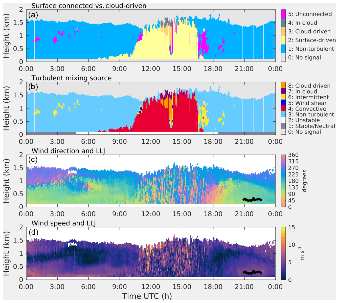
Figure 4 Time–height plots of atmospheric boundary layer classification using the Manninen et al. (2018) scheme showing (a) whether mixing is connected to the surface or cloud driven and (b) the turbulent mixing source, together with time–height plots of (c) wind direction and (d) wind speed on 28 August 2017 at Jülich, Germany. The black lines in (c) and (d) show low-level jet (LLJ) altitude (Tuononen et al., 2017).

Building on the profile-based classification approach from Harvey et al. (2013), Manninen et al. (2018) developed a pixel-based ABL classification scheme that exploits several atmospheric quantities derived from DWL observations. An example of a clear-sky case (Fig. 4) illustrates the complexity in ABL dynamics with diurnal variations clearly detectable from the profile data (Manninen et al., 2018). Unstable atmospheric conditions drive the CBLH morning growth in two stages (Fig. 4a, b), i.e. the slow increase of near-surface convective conditions followed by a rapid growth phase (Halios and Barlow, 2017). The gradual decay of convective activity in the evening transition is clearly detected (Fig. 4a, b). An LLJ forms at some point after sunset (Fig. 4c, d).

Based on profiles of the aerosol scattering ratio derived from ALC measurements, the complex ABL dynamics in an Alpine valley were classified, which proved valuable for the assessment and understanding of local air quality conditions (Diémoz et al., 2019a, b). Through studies that group aerosol or trace gas profile observations according, for example, to turbulence, stability, or LLJ regimes (e.g. Su et al., 2020; Klein et al., 2017, 2019; Dieudonné et al., 2013), characteristic features are starting to emerge that can be very valuable for the assessment of near-surface air pollution concentrations. The gained process understanding of such synergy applications that combine multiple atmospheric variables means ABL classifications are increasingly able to account for the complex interactions of the processes that drive ABL dynamics and atmospheric composition.

5 Conclusions

Despite the importance for a range of applications, quantitative knowledge on the temporal and spatial variations in atmospheric boundary layer (ABL) height is still scarce. While synchronised radiosonde data have provided an immensely valuable assessment of conditions at the global scale for decades now, their comparatively low temporal resolution means they often do not capture diurnal and seasonal variations in ABL dynamics at a given location (amongst other limitations). Thanks to advances in ground-based remote-sensing, high-quality profile observations spanning the ABL extent at very high temporal resolutions are now increasingly collected by operational measurement networks. As these data start to resolve spatio-temporal variations in ABL dynamics even in complex environments such as mountainous terrain or cities, they provide valuable contributions to international research projects in these domains, such as the EU H2020 Green Deal projects RI-URBANS (https://riurbans.eu/, last access: 12 January 2023; ACTRIS) and ICOS-cities (https://www.icos-cp.eu/projects/icos-cities-project, last access: 12 January 2023; ICOS) or the WWRP-Endorsed Project TEAMx (http://www.teamx-programme.org/, last access: 12 January 2023).

As dense measurement networks are emerging across Europe and other parts of the world with high spatial coverage, harmonisation of operations, data processing, and layer height retrievals are key. International operational networks (such as E-PROFILE, ACTRIS, ICOS, ARM) not only collect and archive the observations but also strive to harmonise sensor settings and standardise file formats. Further, coordination between different sensor networks receives increasing attention as this clearly benefits synergy applications. Close collaborations with NHMS, academia, and instrument manufacturers are vital to formulate and implement standard operating procedures, to closely monitor house-keeping data, and to develop both detailed correction procedures and advanced data products, such as the heights of the ABL sub-layers. In Europe, several EU COST actions were paramount for the exchange of knowledge and best practices, including Action 710 (Harmonisation of the pre-processing of meteorological data for atmospheric dispersion models; Seibert et al., 2000), EG-CLIMET (European Ground-based observations of essential variables for CLImate and METeorology; Illingworth et al., 2015), and TOPROF (Towards Operational ground-based PROFiling with ceilometers, Doppler lidars and microwave radiometers for improving weather forecasts; Illingworth et al., 2019). Following the progress made in this field over recent decades, the action PROBE (http://www.probe-cost.eu/, last access: 12 January 2023) (PROfiling the atmospheric Boundary layer at European scale; 2019–2023; Cimini et al., 2020) focuses on the harmonisation of operational procedures, which is necessary to also ensure higher-level products are comparable across Europe and even globally.

This review outlines how ground-based remote-sensing methods are best exploited in order to gain a detailed understanding of ABL sub-layer heights and dynamics. Firstly, the capabilities and limitations of various measurement technologies available to capture different atmospheric profile variables within the ABL are summarised. Choosing the appropriate technology for a given network not only needs to consider the physical information content of the atmospheric quantity observed (temperature, humidity, wind, turbulence, aerosol, or trace gases) but also whether the sensitivity, resolution, and capabilities of a given sensor are appropriate to monitor the layer(s) of interest. Such instrument characteristics not only differ between sensor types but also between models from different manufacturers and can even depend on firmware, hardware, instrument settings, instrument age, or sampling strategies.

Certain ground-based remote-sensing instruments are especially suitable for the operation in automatic measurement networks as these systems are compact, tend to have comparatively lower costs, and can be operated with low maintenance under all (or most) weather conditions. Specifically, these are (i) microwave radiometers (MWRs) and infrared spectrometers (IRSs) for the profiling of temperature (and humidity), (ii) (scanning) Doppler wind lidars (DWLs) or radar wind profilers (RWPs) for the observation of wind and turbulence profiles, and (iii) (high-SNR) automatic lidars and ceilometers (ALCs) for aerosol profiling in the ABL. Further, the deployment of differential absorption lidars (DIALs) in organised sensor networks increase in the future, adding profile observations of humidity or various trace gases.

Numerous methods are available to derive the height of the ABL and its most prominent sub-layers, namely the mixing boundary layer height (MBLH) and the height of the residual layer (RLH). The MBLH represents the stable (SBLH) or convective boundary layer height (CBLH), depending on atmospheric stability conditions. In addition to layer height retrievals, methods are discussed which characterise the ABL based on atmospheric profile observations according to atmospheric stability and turbulence, cloud dynamics, or aerosol distributions. An overview is provided on the capabilities and limitations of the large number of layer height retrievals, including thermodynamic methods, wind and turbulence retrievals, and those based on aerosol information. Retrievals based on temperature and turbulence (or wind) can take into account the atmospheric stratification of the probed layer and are hence able to specifically address either SBLH or CBLH. The height of the surface-based temperature inversion (SBIH) can further be determined from temperature profile data, while a low-level jet can be diagnosed from wind observations. Aerosol-based methods again analyse the result of recent physical and chemical processes, including mixing, advection, aerosol formation, accumulation, or hygroscopic growth and are able to track both MBLH and RLH. They are not suitable to determine the cause of the change in aerosol vertical characteristics, e.g. whether the tracers were transported as a result of thermal buoyancy or shear-driven turbulence. The RLH can also be assessed based on the height of the capping inversion (CI) in a temperature profile.

For the detection of shallow layers, the near-range capabilities of a ground-based remote-sensing profiler are critical while the signal strength (in relation to the noise levels) determines the maximum range observed and data quality within a deep CBL, which can reach several kilometres (3 km or even higher). Sodars tend to have their strength in the near range (mostly within the first kilometre), while high-power aerosol research lidars provide high-quality data at greater altitudes and are not very suitable for the assessment of conditions very close to the surface. For lidar systems, there is usually an inverse relation between limitations in the near and far range because high laser power associated with quality observations at greater altitudes usually goes along with a larger blind zone near the instrument. For DWL, RWP, ALC, or DIAL, a variety of instrument models is available, with respective range extent capabilities and noise levels. Observations in the blind zone of a vertical profile from a scanning DWL can be obtained by including shallow-angle scan strategies. MWRs are very suitable for the assessment of conditions near the ground, given that their sensitivity is maximal near the sensor and the vertical resolution of their temperature product reduces with increasing altitude. For all systems, studies show that careful processing and detailed quality control are vital to produce high-quality profile observations. This is particularly critical for measurement uncertainties that propagate to the accuracy of ABL height retrievals. Naturally, all retrievals are challenged at times when the ABL is dominated by larger-scale, synoptic processes (such as frontal passages), when layer heights are less clearly defined.

The morning growth and evening decay of the CBL pose severe challenges to numerical simulations for a range of applications, including air quality, greenhouse gas assessment and numerical weather prediction. When using observations for model evaluation or comparisons, it is crucial to carefully consider the specific uncertainties in the respective measurement used. Also, it is important to understand which atmospheric variable is used for layer detection, as it can introduce systematic biases, for example if turbulence-derived layer heights are compared to results exploiting aerosol profiles.

Given the different stages of CBL development during morning growth, the continuous monitoring enabled by remote-sensing profilers is a clear advantage for the characterisation of this period compared to balloon ascents. Profiles from sodar or certain ALCs have proved very useful to capture the onset of the CBLH at very low altitudes (< 100 m). Approaches based on high-frequency variations in wind or aerosol characteristics are often particularly good at tracking CBLH during morning growth. Turbulence-based results from RWP usually require longer integration times compared to DWL or ALC that range on the order of minutes. Turbulence- and aerosol-based CBLH results can be very similar during morning growth provided appropriate layer attribution is performed. However, several studies report a temporal delay in aerosol-derived CBLH morning growth both relative to temperature-derived CBLH and turbulence-derived layers, with time lags of up to 2 h. No clear picture has yet emerged on a potential time lag between the growth of temperature- and turbulence-derived layer heights. Method synergy of high-resolution observations (both in time and vertical dimension) is a promising means to better understand and quantify the CBL growth.

Most methods show very good performance during daytime, especially when the CBL is fully developed over the entire ABL. Provided that there is a sufficient SNR and careful data processing, CBLH from all retrieval methods can agree within a few hundred metres. A thick entrainment zone (EZ) can result in a weaker delineation at the CBLH, increasing uncertainty in layer detection for all methods. As convective clouds can significantly challenge layer detection, daytime maxima of the layer estimates from temperature-,turbulence-, and aerosol-based methods are most similar in cloud-free conditions. However, strong shear layers or elevated aerosol layers above the ABL can also challenge turbulence-based and aerosol-based algorithms, respectively.

Although CBLH growth rates and maxima are strongly affected by clouds, the majority of ABLH climatology studies to date focus on clear-sky conditions. Cloud cover or even cloud type are considered very rarely. Recent developments in automatic detection algorithms that now consider cloud dynamics are expected to enable more comprehensive assessments in the future. Especially differentiating between boundary layer clouds and those decoupled from the ABL greatly aids interpretation.

The evening transition of the daytime CBL into the nocturnal boundary layer around sunset is directly monitored by turbulence profiles. While turbulence-based layer retrievals and thermodynamic methods are in general agreement at this time of day, aerosol-based MBLH results are particularly uncertain at this point when aerosol distributions are less suitable to trace the fading turbulence activity. Reliable data in the near range, careful processing algorithms, and high surface aerosol emission rates increase the likelihood of meaningful results from aerosol-based layer detection at this transition time.

The detection and interpretation of nocturnal layer heights is still prone to significant uncertainty. On average, uncertainty in SBLH detection is estimated to be around 30 %–40 %. Further investigation is required into the impact of ABL dynamics and atmospheric stability on the relative agreement between SBLH results. Since turbulence in the SBL is usually not uniform, the diagnosed layer heights can differ systematically between thermodynamic, turbulence, or aerosol-based methods. Most methods are challenged when multiple layers are present simultaneously as the task of layer attribution is considered more uncertain than the simple layer detection step. Hence at night and in the early morning, aerosol-based methods are at risk of confusing MBLH and RLH, especially if the composition is similar within the two layers. Turbulence-based layer detection algorithms may be confused by the presence of intermittent turbulence in the RL. Thermodynamic layer detection from MWR profile data is less suitable for the detection of RLH (given lower sensitivity) so that the RL poses less of a problem for the detection of MBLH at night and in the early morning. The RLH can usually be tracked reliably using thermodynamic retrievals of the CI applied to airborne in situ sensors or by aerosol-based methods, but trace gas observations from DIAL or Raman lidar humidity and temperature observations can also be exploited. At night, instrument synergy between radiometer temperature profiling (IRS, MWR) and aerosol observations from ALC is particularly promising given their respective strengths in observing the SBLH and RLH.

A clear potential is identified for combining multiple methods or observations from multiple sensors (instrument synergy). These can advance both (i) methodologies and products and (ii) process studies and applications.

• i.

  Using the synergy of multiple methods and/or sensors can advance the detection of layer heights and classification procedures.

  • Sensors with different range capabilities can be combined to ensure high-quality data are collected along the entire extent of the ABL.

  • Multiple sensor types can be combined to retrieve atmospheric variables with different physical information content that can then be used to calculate advanced synergy parameters (such as the bulk Richardson number) feeding into the layer height retrieval (combined, for example, by AI or fuzzy logic).

  • Combining layer estimates from a range of methods provides a valuable basis for the assessment of layer height uncertainty, the latter still being a challenging topic due to the lack of an objective reference standard.

  • ABL classification schemes are emerging that not only provide layer heights but also incorporate the source (surface-driven, cloud-driven) or nature (buoyancy, shear) of turbulent exchanges or can differentiate between different aerosol types. Where multiple measurements are combined that represent different physical aspects of the ABL, such tools can be particularly powerful.

• ii.

  Incorporating multiple sensors is extremely valuable for process studies as well as model evaluation.

  • Naturally, utilising multiple sensors across an entire measurement network adds spatial information in the horizontal domain, which allows variations in layer heights to be assessed and interpreted (for example, in relation to surface forcing, local or regional circulations, synoptic conditions) but also for transport processes to be better detected (e.g. horizontal advection within the ABL or long-range transport).

  • Where observations of multiple atmospheric variables are available simultaneously, they allow links between processes to be examined (e.g. understanding the vertical distribution of aerosols as a result of turbulent mixing processes that form in response to the thermodynamic structure of the ABL).

  • Finally, the synergy of multiple sensor networks with different types of profilers that operate continuously starts to portray the four-dimensional complexity of ABL dynamics.

It can be concluded that ground-based ABL profile remote sensing is a powerful means to gain high-resolution observations of the atmospheric boundary layer – to date, the most undersampled part of the atmosphere. The diversity in measurement technology and algorithm variety bears a challenge for the quantification of retrieval uncertainty but should also be considered an advantage for powerful process studies and synergy exploitation of the increasingly rich operational measurement networks.