Seasonally optimized calibrations improve low-cost sensor performance: long-term field evaluation of PurpleAir sensors in urban and rural India

Lower-cost air pollution sensors can fill critical air quality data gaps in India, which experiences very high fine particulate matter (PM_2.5) air pollution but has sparse regulatory air monitoring. Challenges for low-cost PM_2.5 sensors in India include high-aerosol mass concentrations and pronounced regional and seasonal gradients in aerosol composition. Here, we report on a detailed long-time performance evaluation of a popular sensor, the Purple Air PA-II, at multiple sites in India. We established three distinct sites in India across land use categories and population density extremes (in urban Delhi and rural Hamirpur in north India and urban Bengaluru in south India), where we collocated the PA-II model with reference beta attenuation monitors. We evaluated the performance of uncalibrated sensor data, and then developed, optimized, and evaluated calibration models using a comprehensive feature selection process with a view to reproducibility in the Indian context. We assessed the seasonal and spatial transferability of sensor calibration schemes, which is especially important in India because of the paucity of reference instrumentation. Without calibration, the PA-II was moderately correlated with the reference signal (R² = 0.55–0.74) but was inaccurate (NRMSE ≥ 40 %). Relative to uncalibrated data, parsimonious annual calibration models improved the PurpleAir (PA) model performance at all sites (cross-validated NRMSE 20 %–30 %; R² = 0.82–0.95), and greatly reduced seasonal and diurnal biases. Because aerosol properties and meteorology vary regionally, the form of these long-term models differed among our sites, suggesting that local calibrations are desirable when possible. Using a moving-window calibration, we found that using seasonally specific information improves performance relative to a static annual calibration model, while a short-term calibration model generally does not transfer reliably to other seasons. Overall, we find that the PA-II model can provide reliable PM_2.5 data with better than ±25 % precision and accuracy when paired with a rigorous calibration scheme that accounts for seasonality and local aerosol composition.

1 Introduction

Exposure to fine particulate matter, or PM_2.5 (particles with aerodynamic diameter ≤ 2.5 µm), is a leading cause of adverse health outcomes, including premature death (Lepeule et al., 2012; GBD 2019 Diseases and Injuries Collaborators, 2020). India experiences high mass concentrations in both its population-dense megacities and its rural areas, resulting in the largest number of deaths (about 0.98 million annual deaths and about 1.5-year reduction in life expectancy) attributable to ambient PM_2.5 worldwide (Apte et al., 2018; India State-Level Disease Burden Initiative Air Pollution Collaborators, 2021). In particular, New Delhi, the surrounding Delhi National Capital Region, and the broader Indo-Gangetic Plain of north India occasionally experience hourly concentrations exceeding 1000 µg m⁻³ (Gani et al., 2019), resulting in ill health effects even from short-term exposure (Gupta et al., 2021; Krishna et al., 2021). South India generally experiences lower PM_2.5 concentrations but still has population-weighted annual mass concentrations that exceed World Health Organization (WHO) recommendations by a large margin (Apte and Pant, 2019). As relatively fewer polluted megacities in south India continue to rapidly grow, the challenge of ambient PM_2.5 will also increase (Guttikunda et al., 2019; Ramachandra et al., 2020).

Given the high exposure burden and complexity of PM_2.5 throughout India, there is a need to increase understanding of the spatiotemporal patterns of air pollution. Traditional regulatory monitors are expensive to install and maintain, as they require specialized teams and consistent power to maintain networks (Brauer et al., 2019). As a result, there is a dearth of monitors in India (Brauer et al., 2019; Martin et al., 2019). Although satellite remote sensing can fill in the spatial gap, it lacks high-quality temporal coverage and relies on ground-based monitoring for calibration algorithms (Hammer et al., 2020), which can, as is the case in India, result in biased estimates of surface PM_2.5 (Dey et al., 2020).

Starting in around 2010, advancements in miniaturized electronics and laser technology have resulted in the growth of low-cost (< USD 500) PM_2.5 sensor technologies. These light-scattering monitors are popular within the research community and among citizen scientists. The company PurpleAir (PA) has been especially successful in developing (1) a USD 200–280 low-cost sensor that utilizes a commercially available, light-scattering sensor developed by Plantower (PMS5003); and (2) a platform for individuals and organizations to share data from indoor and outdoor PurpleAir low-cost sensors.

Light-scattering low-cost sensors require extensive data quality control and careful selection of calibration models to offer measurements comparable to reference quality instruments (Hagan and Kroll, 2020; Hagler et al., 2018). Optical sensors inaccurately estimate mass from aerosol scattering properties, since PM_2.5 is a mixture of particle sizes and chemical compositions, thus resulting in spatiotemporal variability in optical properties (Hagan and Kroll, 2020; Levy Zamora et al., 2019; Zou et al., 2021). The roles of relative humidity, mass concentration range, sensor aging, and diverse source profiles have been extensively studied in laboratories and field conditions in the USA, Australia, and Europe. Lab studies report that the Plantower sensors do not adequately characterize fine particles above 0.8 µm (Kuula et al., 2020), deteriorate under extreme mass concentrations (Mehadi et al., 2020; Tryner et al., 2020), and are vulnerable to overestimation at RH greater than 60 % (Jayaratne et al., 2018).

Field studies in low to moderate pollution environments show that PA units can be calibrated to reference instruments using simple empirical regression techniques with environmental variables (Barkjohn et al., 2021; Malings et al., 2019; Zheng et al., 2018). Models are often specific to a season and location; however, Barkjohn et al. (2021) demonstrated that a continental USA calibration equation could be effectively deployed for daily data.

Recently there has been increased interest in understanding low-cost sensor performance in the Global South to fill major monitoring gaps (Bai et al., 2020; Jha et al., 2021; Malyan et al., 2023; McFarlane et al., 2021; Puttaswamy et al., 2022; Sreekanth et al., 2022; Zheng et al., 2018, 2019). In north India, Zheng et al. (2018) deployed Plantower models in Kanpur, Uttar Pradesh, for 90 d and found that multilinear regression improved Plantower performance, albeit with significant error for hourly data. In south India, Puttaswamy et al. (2022) calibrated Plantower units for 68 d in Chennai and found a multilinear regression approach that reduced uncertainty to within 15 % and 18 % for PM_2.5 and PM₁₀, respectively. Low-cost sensor studies in India report the importance of climate and emissions variability on aerosol characteristics and advise future deployments to test calibration algorithms across longer timelines (Malyan et al., 2023; Puttaswamy et al., 2022; Sreekanth et al., 2022; Zheng et al., 2018, 2019).

In this study, we deployed and evaluated PurpleAir PA-II sensors in Delhi, Hamirpur, and Bengaluru by collocating with regulatory-grade instruments for 335, 154, and 312 d, respectively. We built hourly local calibration models using multilinear regression. With proper data quality constraints, a relatively simple calibration model can produce high-accuracy and low-bias data. Despite this success, model performance degrades when attempting to transfer a model trained in each environment to data collected in a dissimilar environment. We found a more pronounced reduction in performance when attempting to transfer a model trained in one season to another season, as aerosol characteristics can shift rapidly – even at the same site. Our work demonstrates that low-cost sensors are a viable option for measuring spatiotemporal trends throughout India, but calibration models are vulnerable to the local and seasonal effects on aerosol properties.

2 Methods

2.1 Low-cost sensors

The sensor used in this study was the PurpleAir PA-II. The PA-II is marketed as PurpleAir's outdoor aerosol monitor and is composed of a weatherproof plastic shell containing two Plantower PMS5003 sensors (labeled as A and B channels), an Adafruit model BME280 atmospheric sensor (temperature, RH, and pressure), and a wireless transmitter module to upload data via Wi-Fi. The PMS5003 reports the particulate matter (PM) mass concentrations (µg m⁻³) of all particles with an aerodynamic diameter smaller than 1, 2.5, and 10 µm, as well as particle number concentrations (dL⁻¹) of all particles larger than 0.3, 0.5, 1.0, 2.5, 5, and 10 µm (Zhou and Zheng, 2016).

PurpleAir reports mass concentrations from PA-II models in three forms, which are referred to as CF1, ATM, and ALT. CF1 (correction factor 1) is the “uncorrected” data from the Plantower. The CF1 data have been demonstrated to strongly correlate with collocated integrating nephelometer data (Ouimette et al., 2021). ATM or atmospheric-corrected data use a piecewise function to attempt to account for overestimation. Figure S1 in the Supplement illustrates this function across the full dynamic range for the data collected in Delhi. Between 0 and 20 µg m⁻³, the CF1 and ATM data are 1:1, between 20 and 100 µg m⁻³ the ATM to CF1 ratio transitions from 1:1 to approximately 0.66:1, and at greater than 100 µg m⁻³ the ATM to CF1 ratio is stable at 0.66:1. Although it is reasonable to hypothesize that the ATM data may better represent exposure ambient PM_2.5 than the CF1 data, there is no transparent reasoning in the user manual for this design choice (Wallace et al., 2021; Zhou and Zheng, 2016). Finally, the ALT (alternative data reconstruction) data represent a reconstruction of the PM_2.5 data from the particle number data reported by the Plantower. Briefly, the ALT method adds all the particle counts from bins smaller than 2.5 µm and calculates the particle volume concentration, assuming spherical particles. The particle volume concentration is then multiplied by the unit density (1 g cm⁻³) to estimate the PM_2.5 mass concentration. Wallace et al. (2021, 2020) used these data to develop calibration relationships, reporting the ALT data as being more transparent than using the CF1 or ATM data. However, the particle number data are known not to reflect the actual ambient size distribution, since the Plantower PMS5003 is not a particle sizing instrument but rather reflects a modeled size distribution using assumptions for relationships between size bins that are not always accurate for the atmospheric conditions (Ouimette et al., 2021; Hagan and Kroll, 2020; He et al., 2020; Kuula et al., 2020). Figure S1 shows that the ALT to CF1 ratio is approximately 0.15:1. Although the CF1 and ATM data have dominated most calibration efforts (Malyan et al., 2023; Puttaswamy et al., 2022; Barkjohn et al., 2021; McFarlane et al., 2021; Magi et al., 2020; Malings et al., 2019), the usage of ALT data continues to propagate in peer-reviewed literature (Wallace and Zhao, 2023; Wallace and Ott, 2023). Therefore we use CF1, ATM, and ALT in our study to work towards harmonizing a calibration approach for PA-II in India.

2.2 Regulatory-grade monitors

We compared our PurpleAir measurements against U.S. Environmental Protection Agency (EPA) Federal Equivalent Method (FEM)-certified continuous monitors. Our selected FEMs are Met One Instruments, Inc., BAM (beta attenuation mass monitor) models 1020 and 1022, which are widely used devices (Hall and Gilliam, 2016) that use the beta wave attenuation technique to determine particle mass based on a sample deposited on a filter tape. The FEM certification applies to 24 h averaged data, while the BAM models can provide measurements at hourly or higher time resolution. We used the 1 h block as our highest level of temporal resolution, similar to other low-cost sensor calibration studies using beta attenuation reference monitors in the USA and India (Johnson et al., 2018; Magi et al., 2020; Sreekanth et al., 2022; Zheng et al., 2018).

At the Delhi site, we used the BAM 1020 model; data from this monitor are public and maintained by the U.S. Department of State's AirNow service (San Martini et al., 2015). The Hamirpur and Bengaluru sites utilized the BAM 1022 model managed in collaboration with field teams from the Indo-Gangetic Plains Centre for Air Research and Education and the Center for Study of Science, Technology, and Policy, who manually retrieved data at regular intervals. Staff at each site followed the manufacturer's recommended operation and maintenance, which resulted in downtime for each dataset.

2.3 Deployment sites

Three separate long-term measurement efforts were conducted to evaluate the PA-II performance under different meteorological and aerosol composition regimes. Each campaign was scheduled to last approximately 1 year, enabling a comparison of a range of mass loadings and the effect of season. We use the definition of four seasons from the Indian Meteorological Department (IMD), namely winter (January and February), pre-monsoon (March, April, and May), monsoon (June, July, August, and September), and post-monsoon (October, November, and December; Dubey et al., 2021). A reference map of the collocation sites is presented in Fig. S2.

2.3.1 U.S. Embassy, New Delhi, National Capital Territory of Delhi, India

The Indian National Capital Region, including the capital city of New Delhi (elevation of about 230 m), is the second-largest megacity in the world, with a metro-area population of around 28.5 million people. It has also been called the most polluted megacity in the world, experiencing annual average PM_2.5 concentrations exceeding 120 µg m⁻³ (Fig. S3; Gani et al., 2019). The National Capital Region, along with the rest of north India experiences dynamic meteorology, with cold and wet winters, warmer and drier post-monsoons and pre-monsoons, and hot and wet monsoons (Fig. S4).

Our measurement site was the U.S. Embassy (28.5975^∘ N, 77.1878^∘ E) in the Chanakyapuri neighborhood of central New Delhi. The embassy is located within the city's spacious diplomatic enclave, which has abundant green space, relatively low traffic flows, and minimal local industrial emissions. We collocated 2 PA-II units with the embassy BAM from July 2018–April 2020. During the course of our campaign, Delhi experienced extreme PM_2.5 concentrations during the post-monsoon agricultural burning seasons and characteristic winter inversion layers, with a relatively low-pollution monsoon season, consistent with expected seasonal trends (Guttikunda and Gurjar, 2012).

2.3.2 Indo-Gangetic Plains Centre for Atmospheric Research and Education, Hamirpur, Uttar Pradesh, India

We established a rural PM_2.5 monitoring site in the Hamirpur district, located within north India, in India's most populous state of Uttar Pradesh (UP). Our monitoring site was established in partnership with the Indo-Gangetic Plains Centre for Atmospheric Research and Education. This remote, solar-powered rural monitoring site is situated on a rooftop (20 m above ground level) of a solitary building (25.9552^∘ N, 80.1522^∘ E) located about 800 m outside Ruri Para village in Hamirpur district, Uttar Pradesh. The immediate surroundings within 500 m of the site are a mixture of agricultural fields, ravines, and scrubland forests. The closest major town, Hamirpur (population about 35 000) is approximately 30 km away from the site, and the closest large city, Kanpur (population about 3 million) is 80 km away. Meteorological patterns are similar to Delhi (Fig. S5). We collocated three PA-II sensors with a BAM 1022 model on the Indo-Gangetic Plains Centre for Atmospheric Research and Education rooftop beginning in January 2020. Here, we report on data for the year from January 2020 to January 2021.

Although campaign-median PM_2.5 concentrations at the site (Table 1) are high in the global context, this site's remote location outside of both cities and villages means that the concentrations do not reach the same peaks as in Delhi. However, there are still many local sources of aerosol air pollution in rural north India, such as biomass burning for cooking and heating (Rooney et al., 2019). The Hamirpur dataset is additionally differentiated from the Delhi dataset in that most of the data were collected during the first year of the COVID-19 pandemic, which was observed to change patterns of emissions throughout India (Patel et al., 2021; Singh et al., 2020).

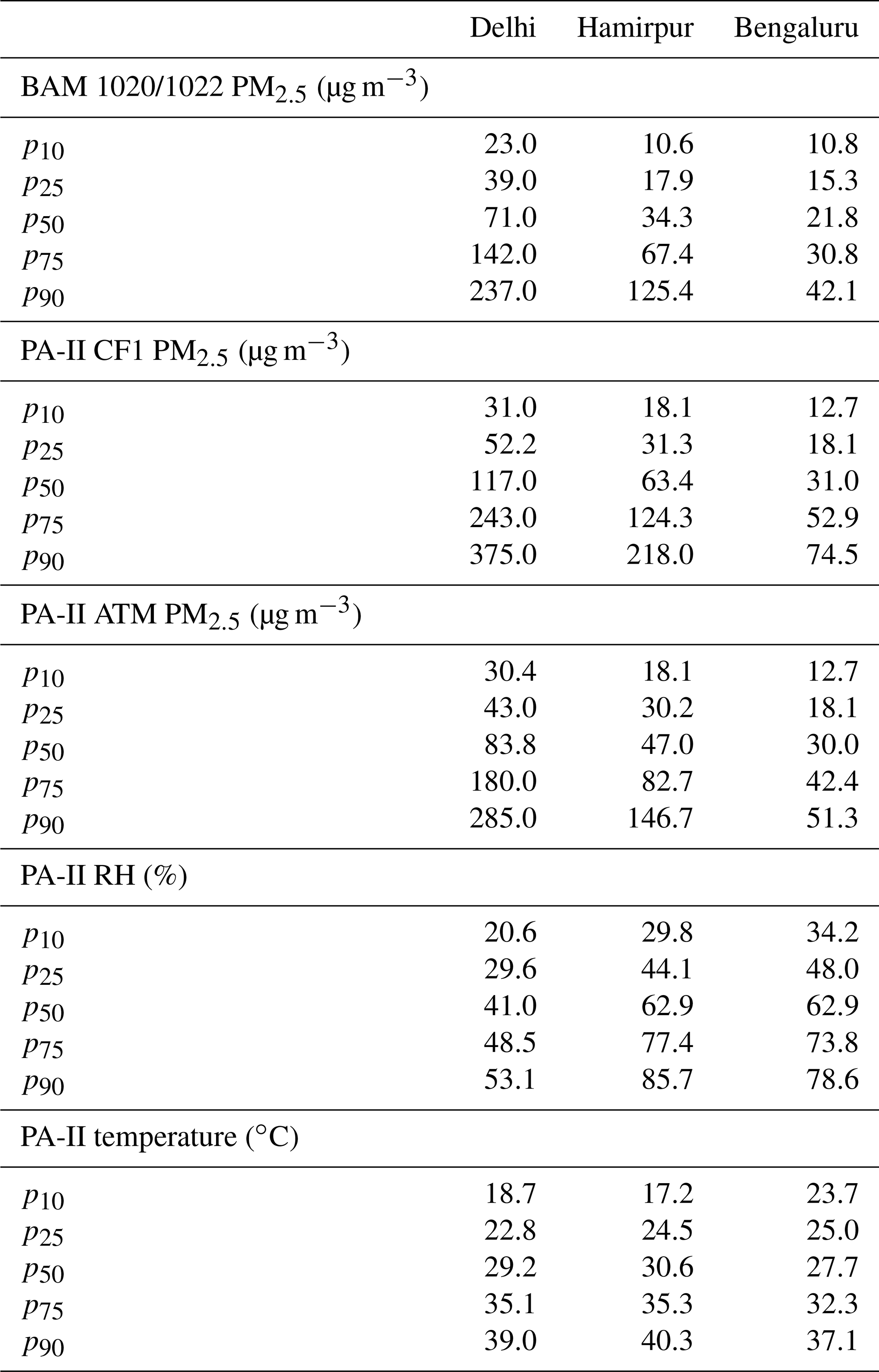
Table 1 Summary of campaign measurements (quality assured according to methods outlined in Sect. 2.4 and summarized in Sect. 3.1–3.3), including 10th percentile (p₁₀), 25th percentile (p₂₅), 50th percentile (p₅₀), 75th percentile (p₇₅), and 90th percentile (p₉₀) for the campaign periods (Delhi from July 2018–April 2020; Hamirpur from January 2020–January 2021; Bengaluru from June 2019–August 2020).

2.3.3 Center for Study of Science, Technology, and Policy, Bengaluru, Karnataka, India

Bengaluru, in south India, is the third-largest city in India, with a population of 8.4 million, and the capital of Karnataka. South India experiences different meteorological conditions and considerably lower air pollution burdens than north India (Apte and Pant, 2019; Dubey et al., 2021) (Figs. S6, S7). Although continuous PM_2.5 regulatory monitors are sparse in Bengaluru, the current network estimates a citywide annual average of 30 µg m⁻³. While the annual average is low in comparison to Delhi and the Indian National Ambient Air Quality Standard of 40 µg m⁻³, it exceeds the WHO annual guideline value of 5 µg m⁻³, and hourly winter concentrations often exceed 50 µg m⁻³. Consequently, Bengaluru has been designated for air quality improvement under the Indian National Clean Air Programme (Ganguly et al., 2020). In Bengaluru, emissions are dominated by traffic and dust resuspension (Guttikunda et al., 2019). Compared to Delhi and Hamirpur, winters are milder, and the climate is more consistent year-round in Bengaluru (Fig. S6). The winter and pre-monsoon seasons are distinguished from the monsoon and post-monsoon seasons primarily by RH and precipitation. Monsoon and post-monsoon are cloudy and rainy, with RH typically exceeding 70 % all day and possibly remaining above 90 % before sunrise. Winter and pre-monsoon RH are more moderate, with hourly averages fluctuating between 40 % and 80 %.

Our collocation site was the Center for Study of Science, Technology, and Policy office in northern Bengaluru. We maintained a BAM 1022 model on the rooftop of a three-story office building (13.0485^∘ N, 77.5795^∘ E). Although the site is located near a highway (Outer Ring Road), the annual diurnal patterns matched the regional signature from the average of the regulatory monitors. Furthermore, the area surrounding the site is mostly office buildings, with some residential housing. There are no large industrial sites or obvious large point sources in the neighborhood, other than occasional small solid-waste fires. It is likely that the Bengaluru BAM is thus mostly influenced by urban background and regional aerosol conditions. We set up two PA-II sensors from June 2019–July 2020, during which Bengaluru experienced hourly spikes above 100 µg m⁻³ during the festival of Diwali and dynamic changes in traffic patterns due to the COVID-19 pandemic and lockdowns.

2.4 Quality assurance

2.4.1 PurpleAir PA-II PM_2.5

Many light-scattering PM_2.5 sensors, including the PA-II, can report unrealistic measurements, lack accuracy (especially at high mass loadings), and are only recommended for operation within a specific range. To minimize these effects, we removed unreasonably small and large points (outside the range of 5–500 µg m⁻³), averaged each individual Plantower unit by the hour, averaged across all units for a given site, removed imprecise points, and calibrated the resulting clean dataset. We conducted quality assurance (QA) procedures separately for each sensor correction factor (CF1, ATM, and ALT).

We removed all raw PM_2.5 data points outside of the range 5–500 µg m⁻³ (Kelly et al., 2017; Magi et al., 2020; Zhou and Zheng, 2016). Analyses of PurpleAir data typically report the percent error between channels A and B for a given unit to remove imprecise points, thus treating them as joint measurements and all other nodes as independent (Barkjohn et al., 2021). However, at our collocation sites, there was always more than one PA-II, so we treated all Plantower sensors as replicate measurements and averaged them together as a single data point. For instance, if we had three PA-IIs at a site, then we averaged the six values together – two from each unit – to estimate a single data point. We established 80 % completeness criteria (or 24 2 min data points) for each hourly average and at least two valid Plantower hourly averages for the resulting site PA data point. Imprecise data points were removed using the coefficient of variation (CV), the quotient of the standard deviation, and the mean of the collocated Plantower sensors for a given 2 min raw sample. CV values greater than 0.2 were removed, which is broadly consistent with approaches used by other studies (Badura et al., 2018; Crilley et al., 2018).

2.4.2 PurpleAir PA-II temperature and relative humidity

The Adafruit model BME280 is considered to be a reliable and accurate low-cost environmental sensor (Araújo et al., 2020). There are occasional incidents of sensor miscommunication with the microprocessor, leading to unrealistic values, which we filtered out by restricting RH to 0 %–100 % and temperature to −10 to 50 ^∘C. We computed the dew point temperature from the measured temperature and RH, following Malings et al. (2019).

2.4.3 Met One BAM 1020 and BAM 1022

The BAM instrument flags low-quality data with a specific code to (1) potentially remove them from analyses and (2) diagnose underlying issues, which can include power loss and pump errors. The default concentration range of the BAM 1020 and BAM 1022 models is 3–1000 µg m⁻³. Unlike the PA-II, the hourly limit of detection of the BAM 1022 and BAM 1020 is well constrained to 2.4 µg m⁻³ (Magi et al., 2020), which is considerably below the typical concentrations in our dataset. Like other linear regression studies using Met One BAM models and Plantower nephelometers, we utilized an ordinary least squares approach (Barkjohn et al., 2021; Malings et al., 2019; McFarlane et al., 2021; Mehadi et al., 2020; Wallace et al., 2021; Zheng et al., 2018).

2.5 Calibration regression

Since nephelometers and other optical-based sensors are known to provide biased measurements of PM_2.5 measurements relative to reference-grade instruments, in large part due to hygroscopic growth, calibration procedures attempt to account for bias due to RH, index of refraction, and mischaracterizing the particle size distribution. One approach is to leverage the environmental data (RH, temperature, etc.) from low-cost sensor nodes to develop the best-fitting model without imposing any a priori assumptions about aerosol growth or chemistry (Barkjohn et al., 2021; McFarlane et al., 2021; Malings et al., 2019; Wallace et al., 2021; Zheng et al., 2018). We label this approach as “data-driven”. From decades of work with optical instruments, corrections have been developed by assigning non-linear growth terms as a function of RH and known PM_2.5 chemical characteristics (Malings et al., 2019; Chakrabarti et al., 2004). In our work, we label this approach as “theory-driven”, since it attempts to fuse the best-fitting function form from theory with the best-fitting regression coefficients. Although the theory-driven model should produce the most transferable models, since theory should apply in all environments, the underlying data processing of the Plantower – a truncated nephelometer (Ouimette et al., 2021) – may result in a bias structure that is better explained by a linear RH correction than a non-linear correction for the dynamic range of RH under real-world conditions.

2.5.1 Data-driven model selection

To ensure that our work is easily reproducible within India, we relied only upon variables reported or calculable by the PA-II as independent variables, namely PM, RH, temperature, and dew point. For our PA-II PM_2.5 variable, we evaluated CF1, ATM, and ALT values. We evaluated all regression models using ordinary least squares, with the BAM PM_2.5 as the dependent variable and our candidate parameters as independent variables. To iterate across all possible arrangements of predictors – including additive terms, interaction terms, and polynomial terms up to the third order – we implemented sequential feature selection (SFS), using the Python package scikit-learn 0.24.2. SFS uses a “greedy” approach to converge on the best-performing model for a user-defined number of parameters (Raschka and Mirjalili, 2019; James et al., 2013; Ferri et al., 1994). For example, if a user wanted a two-parameter model from a set of 10 features, then SFS would iteratively compare 90 models (i.e., the set of all possible two-parameter feature permutations), using a robust regression metric (such as the adjusted R² or Bayesian information criterion, BIC). In our approach, we first use SFS to define the best-performing n-parameter model, starting with all possible parameters (n=34). We then compare the adjusted R² across best-performing n-parameter models to measure the impact of the model complexity. If increasing the parameters results in only marginal improvements (ΔR²≈0.01), then it is unnecessary to use those additional features. The overall most robust model, therefore, reflects both the best possible selection of features and the feature parsimony.

2.5.2 Theory-driven model selection

From the κ-Köhler theory, we expect wet PM_2.5 scattering to increase exponentially with increasing RH, resulting in strongly non-linear dynamics. Therefore, we applied a calibration function relying on empirically fitted coefficients from the training data, with a non-linear RH term to capture the expected trends from the theory. Studies have attempted to apply a non-linear RH term for light scattering low-cost sensors, with results similar to or less accurate than an additive term (Chakrabarti et al., 2004; Malings et al., 2019; Tryner et al., 2020; Zheng et al., 2018). Given the difference in emission sources, size distribution, mass loadings, and meteorology, we decided to include a non-linear RH term, using the following form in Eq. (1).

$$\begin{array}{}\text{(1)}& C={\displaystyle \frac{\mathit{\alpha }\times P}{\mathrm{1}+\mathit{\beta }\frac{{\mathrm{RH}}^{\mathrm{2}}}{\mathrm{1}-\mathrm{RH}}}},\end{array}$$

where α and β represent the regression coefficients to be fitted via non-linear least squares, P is the PurpleAir signal (ATM, CF1, or ALT), RH is the unitless relative humidity scaled from 0 to 1, and C represents the corrected PM_2.5.

2.5.3 Cross-validation

To evaluate our calibration models, we sought to design an appropriate cross-validation scheme that would permit a balanced evaluation of model performance among all seasons. A simple test–train split would likely over-represent seasons with more measurements. We thus performed a stratified k-fold cross-validation, in which each fold contains equal representation from each of the four seasons; we evaluated each model by leaving one fold out in subsequent iterations.

2.5.4 Temporal sensitivity

As a point of contrast with the seasonally balanced calibration described above, we performed a data experiment to investigate the temporal stability of a hypothetical shorter-term calibration. This exercise was motivated by the common practice in many low-cost sensor deployments that perform a short-term initial calibration before deploying sensors in the field and then, if the low-cost sensors are available, perform another short post-study collocation. Previously, Levy Zamora et al. (2023) identified diminishing returns in improvements to calibration regressions after about 4 weeks of collocation in Baltimore, USA, if that period encapsulated a representative range of PM_2.5 and RH conditions. Here we build on this work by seeking to identify which 4-week period is ideal at our sites in India, since annual median PM_2.5 concentrations at the Delhi and Hamirpur sites are about 10× higher than Baltimore and reflect a different mixture of chemical composition and aerosol properties. To explore the potential bias from extrapolating a short-term calibration to a longer period, we fitted 4-week rolling ordinary least squares models with the features selected via SFS and compared the performance against all other 4-week periods during our yearlong data collection to understand the implications of short-term calibration for other studies.

2.5.5 Performance metrics

As a guiding principle, we selected those models which balanced parsimony with low error, low bias, and strong temporal consistency for presentation. We selected analytical methods and performance metrics to optimize these parameters and have designated these best-performing models as being “robust”. Given the high concentrations and high variability within and between sites, we report the normalized root mean square error (NRMSE), allowing a comparison of model performance across sites and time periods (Simon et al., 2012). Additionally, we used the coefficient of determination (R²) to evaluate model accuracy (Simon et al., 2012). For multivariate regression models, we used the adjusted R² metric to account for spurious correlations with increasing numbers of independent variables. To penalize the overfit and minimize the number of parameters, we used the Bayesian information criterion, a metric for parsimonious feature selection (James et al., 2013), when selecting between models during the SFS process. Finally, we assessed the mean bias error (MBE) and normalized mean bias error (NMBE) to characterize the average direction of error (Simon et al., 2012).

3 Results and discussion

3.1 Reference instrument data summary and quality assurance

BAM and PA measurement summary statistics are summarized in Table 1 for each site, with time series plots in Figs. S8–S10. Overall, BAM monitors used at each site provided consistent performance, despite the challenging deployment circumstances due to intermittent power loss; extreme weather, including heavy rains; and a relatively broad range of mass concentrations.

The U.S. State Department monitor in Delhi employs the U.S. EPA's data reduction process (San Martini et al., 2015; Vaughn, 2023), resulting in a loss of about 3 % for the data points, with a continuous gap from 10 February to 18 March 2019. For context, we compared this site's time series with 39 other sites in Delhi's regulatory network and found a R² of 0.86 and a mean difference from the regulatory network average of −8.4 µg m⁻³, likely resulting from this monitor's location in one of the city's cleanest neighborhoods. The diurnal plot for the Delhi BAM in Fig. 1 reflects the roles of time-varying emissions and boundary layer dynamics with peaks during the morning traffic rush hour (07:00–10:00 LT) and extremes in the winter exceeding an average of 200 µg m⁻³ during the night and early morning. During the monsoon, we observed a relatively low daily dynamic range of 35–50 µg m⁻³.

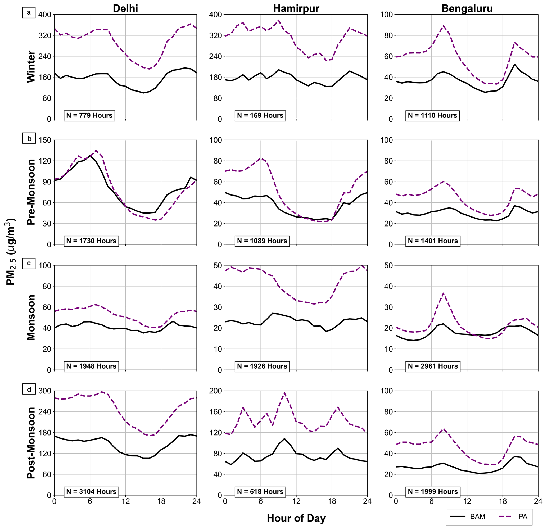
Figure 1 Diurnal profiles of mean hourly seasonal BAM (reference) and uncorrected PA PM_2.5 signals for Delhi, Hamirpur, and Bengaluru, using the CF1 channel. The number of valid hourly averages (quality assured according to methods outlined in Sect. 2.4 and summarized in Sect. 3.1–3.3) in each dataset is presented at the bottom left of each subplot. Winter (January and February), pre-monsoon (March, April, and May), monsoon (June, July, August, and September), and post-monsoon (October, November, and December) are shown. No single hour of the day represents more than about 7 % of the total dataset shown in the bottom-left corner of each plot.

At both the site in Hamirpur and the site in Bengaluru, we used the manufacturer's specified data flags to perform quality assurance, resulting in 6 % and 11 % data loss for the Hamirpur site and Bengaluru site BAMs, respectively. Unlike Delhi, the Bengaluru network is sparse (n=40 in Delhi versus n=8 in Bengaluru), with relatively low data completeness from the official monitors. Diurnal plots in Fig. 1 show a morning peak, with maximum values typically at 08:00–09:00 LT for the collocation site BAM. The closest regulatory monitor to the Hamirpur site is in Kanpur, more than 50 km away, which is too far for meaningful comparisons of local conditions. Figure 1 shows similar trends to the U.S. Embassy site in Delhi, with a morning peak between 07:00–09:00 LT in the morning, extreme mass concentrations throughout the winter, and a low dynamic range during the monsoon. There are no long continuous gaps from this monitor; however, power outages were more frequent in Hamirpur than the other two sites, since it is a rural site, leading to significant data loss – about 14 % of the total campaign hours, concentrated in the pre-monsoon period.

3.2 PA-II quality assurance

We evaluated the unit-to-unit precision of the PA-II sensors by comparing the individual channels of all co-located Plantower sensors at each site. Because each PA-II contains two Plantower sensors, there were always a minimum of four Plantower sensors operating at each monitoring site. The PA-II PM_2.5 channels were highly precise, with a strong correlation (R² ≥ 0.9) both within nodes and between nodes across the mass concentration distribution, which is consistent with the existing literature (Kelly et al., 2017; Levy Zamora et al., 2019; Sahu et al., 2020). Bland–Altman plots indicate high precision across all sites and units, with mean differences centered near 0 µg m⁻³ and most hourly points within ≤ 20 % (Figs. S11–S13). The between-Plantower R² range for the CF1 data across all collocated PA-II sensors was between 0.94–0.99 for the Delhi site, 0.92–0.99 for the Bengaluru site, and 0.95–0.99 for the Hamirpur site (Fig. S14). Disagreement was more pronounced at high concentrations (>100 µg m⁻³) at which R² ranges at each site dropped to 0.90–0.95, 0.83–0.88, and 0.92–0.94 for Delhi, Hamirpur, and Bengaluru, respectively. Similar intra-sensor correlations were found for the ATM and ALT data. Given the consistent between-sensor hourly precision across sites (NRMSE ≤ 10 %), we can confidently state we expect a random error of at most 10 %.

Applying the detection limit thresholds removed 1 % of the total Delhi dataset and <1 % from the Hamirpur and Bengaluru datasets. The CV test removed about 15 % from each site. RH and temperature microcontroller errors were limited to about 4 % of the total data in Delhi and Hamirpur and <1 % in Bengaluru.

After removing the filtered data points, accounting for power losses, and applying the completeness criteria for 1 h hourly averages, the site-averaged PA data resulted in an average coverage of 47 % (n=9260 h), 63 % (n=5958 h), 86 % (n=8567 h) for Delhi, Hamirpur, and Bengaluru, respectively, across CFs. Finally, the reference dataset was synchronized with the PA dataset, and the combined dataset coverage is 38 % (n=7504), 39 % (n=3744), and 75 % (n=7473) for Delhi, Hamirpur, and Bengaluru, respectively. The smaller number of data points available for the Delhi and Hamirpur sites principally arose because of relatively more downtime of the BAM instruments at these two locations.

3.3 PurpleAir data summary

Across sites, the PA-II captured diurnal and seasonal trends with similar results to the collocated BAMs, as evident in Figs. 1 and S15. However, inconsistent biases among the season and location were also observed for all three PM_2.5 channels (CF1, ATM, and ALT), resulting in poor accuracy for the uncalibrated dataset. Although the poor accuracy is unsurprising, our findings highlight the importance of dynamic emissions and meteorology across the Indian subcontinent and field performance at extreme mass concentrations.

In Delhi, the PA data (CF1) correctly identified the winter and post-monsoon periods as being the most polluted seasons, with a strong diurnal range peaking at 08:00–09:00 LT (Fig. 1). The PA also characterized the Delhi monsoon well, with a low diurnal range and a daily average less than 60 µg m⁻³. The uncalibrated low-cost sensor overestimates concentrations during the extremely polluted and humid post-monsoon and winter. There is notably more accurate performance during the dry and hot pre-monsoon, albeit with a tendency to underestimate mass concentrations relative to the reference at least half of the hours of the day. The PA units at Hamirpur follow a similar trend. Although both the Delhi and Hamirpur sites feature relatively low bias in the pre-monsoon period, they underestimate mass concentrations in this season, perhaps due to the influence of wind-blown mineral dust, as observed elsewhere in field and lab evaluations (Jaffe et al., 2023; Kuula et al., 2020; Levy Zamora et al., 2019; Sahu et al., 2020; Sayahi et al., 2019). While crustal material does not generally dominate PM_2.5 mass, during dust storms the lower tail of the coarse-mode aerosol can lead to substantially elevated PM_2.5 concentrations in India.

Since Bengaluru's meteorology exhibits comparatively low seasonality, and emissions are more strongly influenced by mobile sources rather than the more complex mixture in Delhi, low-cost sensor performance is different than in Delhi and Hamirpur. During the day (09:00–19:00 LT), accuracy is biased by more than +25 % during the winter, pre-monsoon, and post-monsoon periods, with systemically lower bias, including underestimates in the less polluted monsoon season (Fig. 1). Accuracy is lower during higher mass loadings at night and during early morning hours, with strong overestimates across seasons peaking during the most polluted hour (07:00–08:00 LT).

3.4 Model selection

3.4.1 Data-driven model fitting

The SFS results are summarized in Table 2 (with extended results in Tables S1–S3 in the Supplement), where the four most relevant parameters are listed in order of decreasing importance for each CF and site. Across sites, R² stabilized at two parameters (about 0.8 for Delhi and about 0.9 for Hamirpur and Bengaluru). For all sites, sensor-estimated PM_2.5 was generally selected as being the single most relevant parameter for predicting concentrations measured by BAM, followed by a variation in the RH (i.e., RH² and RH³). The form of the most robust Bengaluru model is different from the Delhi and Hamirpur sites, with an interaction term between temperature and ALT PM_2.5 (rather than CF1 PM_2.5) being selected as the most predictive PM_2.5 data stream. Furthermore, the Bengaluru dataset ranked temperature and dew point as being more relevant than the Delhi and Hamirpur datasets. Constraining Bengaluru to the same top parameters as the Delhi and Hamirpur sites (CF1 PM_2.5 and RH) reveals only marginal differences (ΔNRMSE ≈ 2 %) in the performance from the most robust model selected by SFS (ALT PM_2.5 and RH³). As such, we choose to standardize our calibration across all sites, with only CF1 PM_2.5 and RH as relevant parameters.

Table 2 Most relevant parameters selected through sequential feature selection for each PurpleAir PM_2.5 channel by site CF1 (uncorrected PurpleAir PM_2.5), ATM (atmospheric-corrected PurpleAir PM_2.5), and ALT (alternative PurpleAir PM_2.5 – reconstructed from the modeled size distribution data). Parameters include relative humidity (RH), temperature (T), and dew point (D).

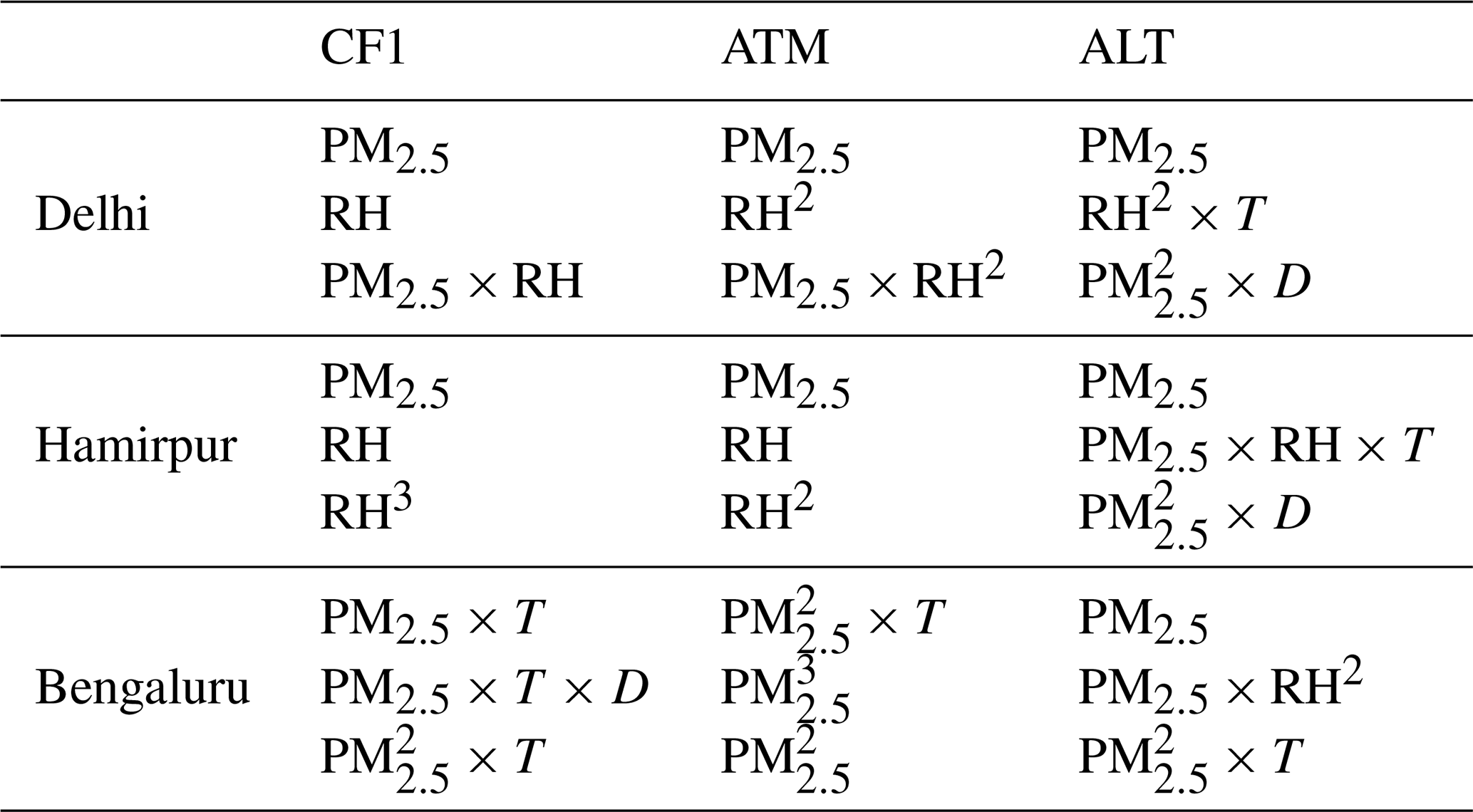
Regression coefficients of the CF1 PM_2.5 data were positive values less than 1, indicating that the CF1 data generally overestimate but are positively correlated with reference monitors. RH term coefficients at the Delhi and Hamirpur sites are negative, indicating that increasing RH should negatively weigh the PA reading, consistent with the expected artifacts of hygroscopic growth in the atmosphere. The Bengaluru dataset similarly assigns RH terms a negative weight. Temperature and dew point terms only imparted marginal improvements to calibration models (ΔR²≈0.01; see Fig. S16), and it is not determinable if the models are deriving a spurious correlation or detecting underlying aerosol or instrument properties.

3.4.2 Theory-driven model fitting

Table S4 summarizes the best-fitting model coefficients from the training dataset for each site and each CF. Across sites, the PM_2.5 regression coefficient (α) does not vary substantially; it is about 14 % for CF1. Hygroscopic growth regression coefficients (β) vary greatly from site to site for CF1, even within the same region; β_CF1 for Delhi is double that for Hamirpur, which is perhaps due to a higher abundance of hygroscopic species (Chen et al., 2022; Gani et al., 2019).

The lack of consistency in fit is reasonable, as the Plantower proprietary algorithm and underlying physical–optical design of nephelometers mean that the sensor does not explicitly account for the underlying aerosol size distribution and composition. The resulting datasets are therefore somewhat divorced from the expected pattern, based on the κ-Köhler theory. The ALT dataset removes the proprietary ATM correction and assumptions of particle density present in the CF1 data, resulting in more consistent β intra-regional values, though with less consistent α values.

3.4.3 Model evaluation

For the Delhi and Hamirpur sites, both located in north India, two-parameter ATM and CF1 models yielded consistent improvements compared to one-parameter models, as summarized in Fig. 3 for Delhi and Hamirpur, respectively. The CF1 models were consistently more accurate than their ATM counterparts in Hamirpur, albeit by about 1 % NRMSE and less than 1 % R². Conversely, in Delhi, the ATM models systematically outperformed the CF1 models by about 1 % NRMSE and R². As evident in Fig. 1, Hamirpur experiences overall lower mass loadings than Delhi. Consequently, the absolute difference between the two signals due to the Plantower piecewise function (Fig. S1) above about 20 µg m⁻³ is likely less important in Hamirpur than in Delhi, where mass loadings are consistently elevated.

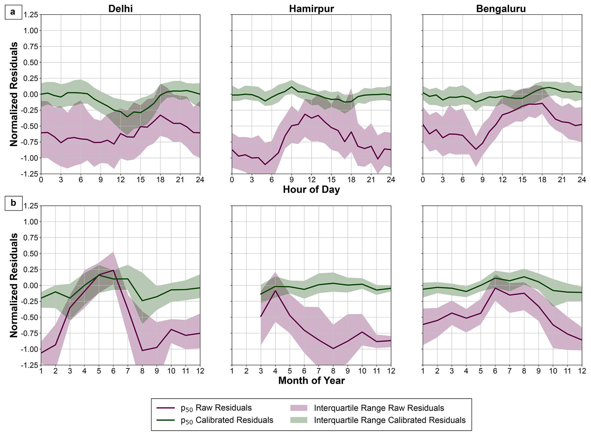
Figure 2 Normalized residual distributions for the uncalibrated PurpleAir data (CF1) and the calibration models for each site. Bold lines represent the median (p₅₀) of the distribution, while the shaded area represents the interquartile range (p₇₅–p₂₅). Panel (a) shows the diurnal distribution, while panel (b) shows the normalized residual distribution binned by month. Compared to the residual distribution for uncalibrated (raw) data, the calibration effectively eliminates most seasonal and diurnal biases.

The theory-driven hygroscopic growth correction consistently improved the performance from the uncalibrated baseline data across sites by 12 % for ATM and 60 % for CF1, on average (Fig. 3). In Delhi and Hamirpur, the theory-driven model performs within about 2 % of the one-parameter models and outperforms the one-parameter ATM model in Hamirpur by 4.3 %.

However, since the Plantower PMS5003 is a nephelometer, the signal should not necessarily follow the expected non-linear hygroscopic growth with increasing RH above 60 %, as expected from a size-resolved measurement technique (Crilley et al., 2020; Hagan and Kroll, 2020). As a result, the two-parameter CF1 models in Delhi and Hamirpur, with their additive RH terms, outperformed the theory-driven model by at least 3 %. In Bengaluru, the theory-driven model performance was comparable to the data-driven models (about 1 % NRMSE; see Fig. 3). This contrast in performance between the two methods in north India is likely a result of the less seasonally variable meteorology and source mixtures in Bengaluru, leading to less dynamic aerosol hygroscopicity.

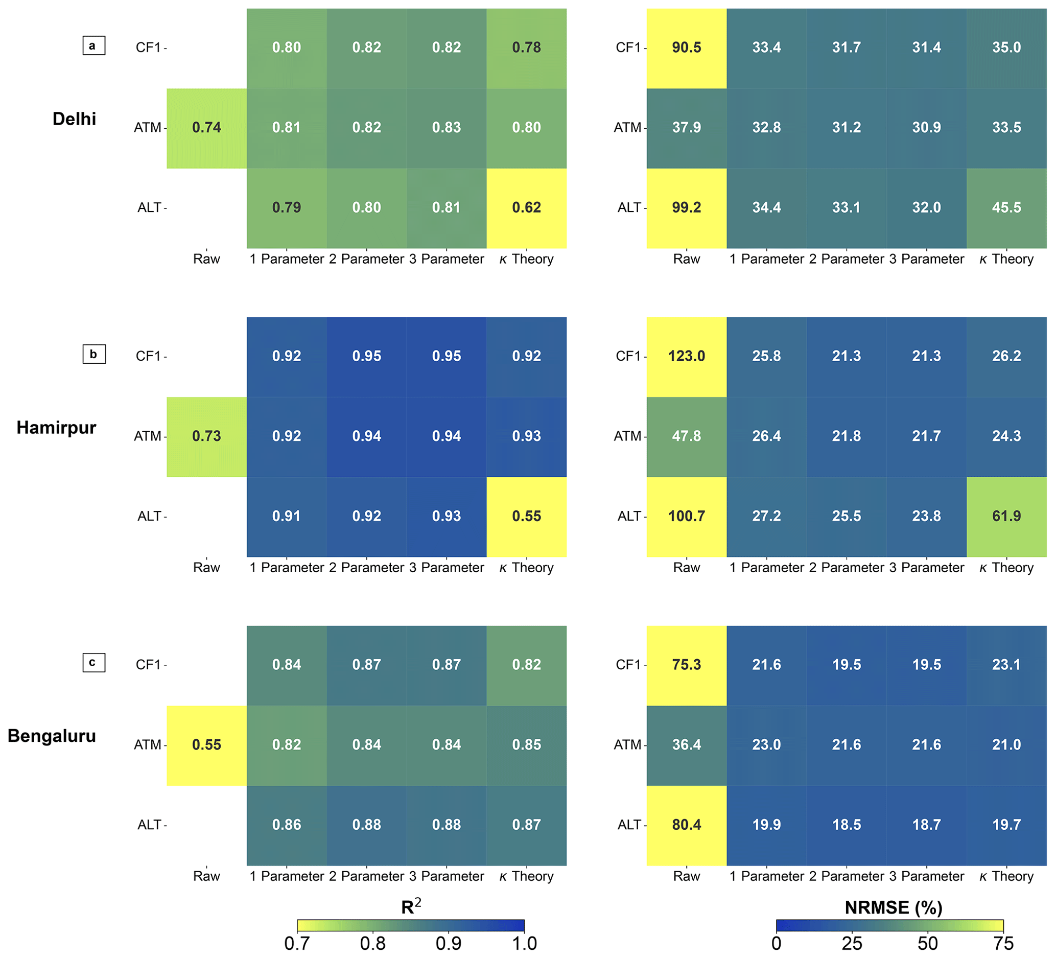
Figure 3 Regression metrics, R² (left) and NRMSE (right), for the raw data, one-parameter model, two-parameter model, three-parameter model, and theory-driven hygroscopic growth model for each PM_2.5 channel (CF1, ATM, and ALT) for each site (Delhi in panel a; Hamirpur in panel b; Bengaluru in panel c). The largest improvements are from the raw data to the one-parameter model, with only marginal improvements in the three-parameter and theory-driven models.

Since CF1 data produce models as accurate as or more accurate than ATM models, have been validated in studies around the world, and do not feature the same non-linear behavior as the ATM channel, we recommend using CF1 for calibration in Delhi and Hamirpur. In Bengaluru, the ALT data may be useful and warrant further study in similar environments, including across south India. From our results, the CF1 data are suitable for deployment in Bengaluru and provide uniformity in calibration guidance. Additionally, the two-parameter model (with RH as additive terms to PM_2.5) follows previous studies (Barkjohn et al., 2021; McFarlane et al., 2021; Zheng et al., 2018) across continents and aerosol regimes. In Barkjohn et al. (2021), the large sample size of PA-II across the continental United States was used to derive a similar calibration regression. In Tables S5–S6, we compare the NRMSE and MBE for our best CF1 model forms from the SFS procedure (up to three parameters), theory-driven CF1 model, and Barkjohn et al. (2021) model output. We have found from our seasonally balanced test dataset that our models perform moderately better (ΔNRMSE of about 5 % across sites) than the EPA model, which is perhaps intuitive, given the differences in PM composition and concentrations in India relative to the USA. Furthermore, the MBEs of our site-specific models are close to 0 µg m⁻³, while the Barkjohn et al. (2021) model systemically suppresses mass concentration estimates, with an MBE as high as 22 µg m⁻³ in Delhi, compared to an MBE of −0.7 µg m⁻³ when using the Delhi site-specific model or 3.25 µg m⁻³ when using the Hamirpur model on the Delhi test dataset. Overall, while the site-specific models we develop here clearly outperform the model of Barkjohn et al. (2021) for these three Indian sites, it is nonetheless striking that this USA-developed calibration still performs quite well at these three Indian sites. Given these findings, we selected the following multi-season correction equations (Eqs. 2–4) for Delhi, Hamirpur, and Bengaluru, respectively. Although relatively simple, our calibration models greatly improve the reliability of low-cost sensor data across aerosol regimes. Figure 2 summarizes each model's bias in at each collocation site, with seasonally and diurnally segregated residuals. Across all sites, the monthly bias of the calibrated data is within ±25 %, in contrast to the uncalibrated data. Figure 3 summarizes model accuracy, with NRMSE improvements from uncalibrated data ranging between 5 %–20 %. Figure S17 additionally explores the residual structure and demonstrates the value of the selected model forms at reducing bias due to RH and mass loading factors. The calibrated residual distributions demonstrate marked improvements across the full range of mass concentrations (5–500 µg m⁻³), unlike the raw residuals, which show increasing uncertainty at high mass concentrations. The selected calibration equations reduce the median bias to near 0 % across sites from a median bias as high as 150 %, using the uncalibrated data at RH > 60 %. Figure 4 summarizes the performance of Eqs. (2)–(4), highlighting that although performance is robust in the aggregate, seasonal and diurnal shifts in aerosol properties can shift performance and uncertainty bounds, therefore motivating further investigation into the role of calibration sensitivity to temporal factors.

$$\begin{array}{}\text{(2)}& {\displaystyle }C=\mathrm{0.546}\times \mathrm{CF}\mathrm{1}-\mathrm{0.936}\times \mathrm{RH}+\mathrm{50.3}\text{ (Delhi)}\text{(3)}& {\displaystyle }C=\mathrm{0.496}\times \mathrm{CF}\mathrm{1}-\mathrm{0.296}\times \mathrm{RH}+\mathrm{22.0}\text{ (Hamirpur)}\text{(4)}& {\displaystyle }C=\mathrm{0.515}\times \mathrm{CF}\mathrm{1}-\mathrm{0.139}\times \mathrm{RH}+\mathrm{14.1}\text{ (Bengaluru)}\end{array}$$

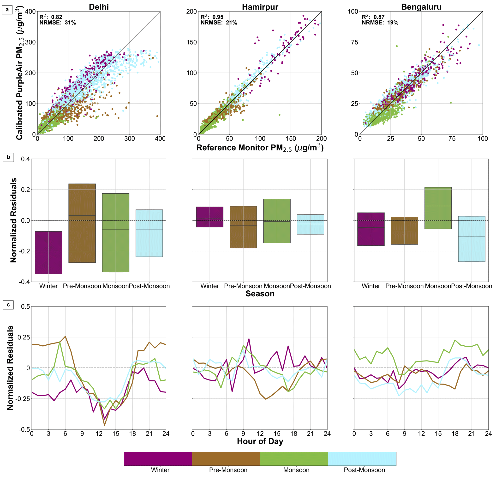
Figure 4 Scatterplots of the best-performing two-parameter annual models for each of the sites in panel (a), with the corresponding normalized model residuals segregated by season in panel (b) and segregated by the time of day in panel (c). In panel (a), the solid line represents unity. In panels (b) and (c), the dashed line represents the normalized residual value of zero. In comparison to Fig. 2a, the normalized diurnal residuals in panel (c) are presented over a restricted y axis, accentuating the residual structure.

3.5 Model evaluation

3.5.1 Temporal sensitivity

To identify the stability of the model and its parameters, we computed the 4-week rolling ordinary least squares (ROLSs) for each of our selected models and compared performance to all other 4-week moving ROLS models. Each model's NMBE across time is shown in Fig. 5, where the gray squares in the top panel indicate less than 50 % data completeness. Additionally, the bottom panel of Fig. 5 tracks the distribution of the diagonal of the matrices present in the top panel of the figure. Across sites, the choice of the calibration period greatly changes the performance of the regression throughout the rest of the dataset and influences the selection of regression coefficients. Figure S18 additionally explores the absolute bias, demonstrating that the biases in Eqs. (2)–(4) are centered near zero. Figure S19 illustrates the same analysis with NRMSE, showing that the monthly ROLS model performance is generally stronger than the annual model within the training month, but that it rapidly deteriorates.

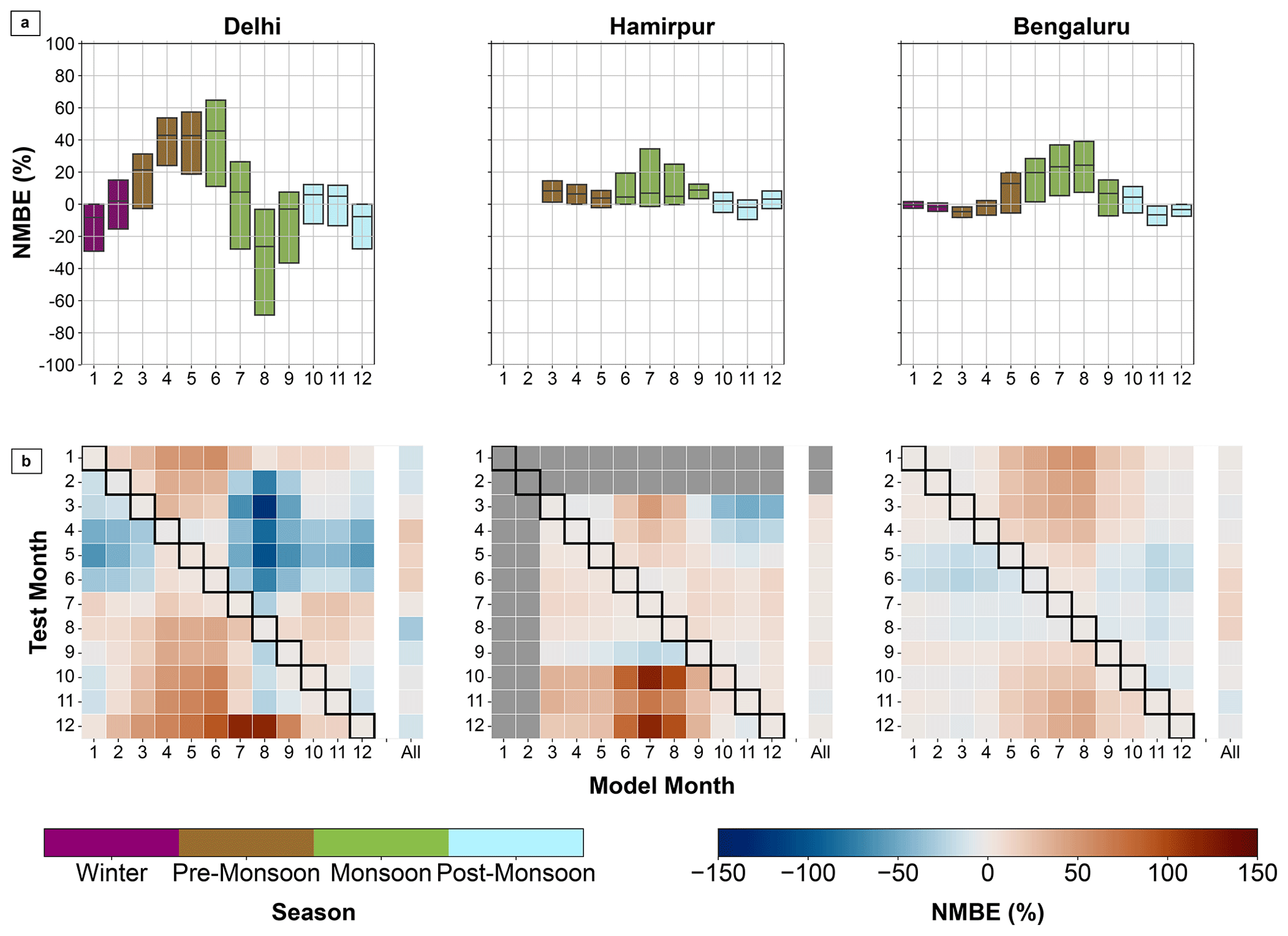
Figure 5 Assessment of inter-seasonal transferability of seasonal models. Panel (a) depicts box plots of the distribution of normalized mean bias error (NMBE) for a given model starting month of a 4-week ROLS model on all other windows. The bottom, solid line, and tops of the boxes represent the 25th, 50th, and 75th percentiles, respectively. Panel (b) presents the median NMBE of a 4-week ROLS model trained to start in the month (colored by season) on the x axis and evaluated on all other windows, as binned by the starting month on the y axis. Gray boxes represent months without sufficient data. Models trained in the pre-monsoon period underpredicted in other seasons, contrary to the typical pattern of overprediction – this pattern is consistent at Delhi and Hamirpur. As a point of comparison, we present the performance of our long-term calibration in individual months at each site in the column (b) labeled “All”, which is consistent with our observation that 4-week models trained in a single month generally do not perform as well in other months.

In Delhi, model performance and coefficient selection exhibit a seasonal pattern, with post-monsoon and winter month models (January, February, March, September, October, November, and December) performing well and selecting similar regression coefficients even across years (Fig. S20). When evaluating model performance on data within the same season, NRMSE is typically below 30 %, and R² is above 0.7. However, the post-monsoon and winter models perform poorly when evaluated on pre-monsoon data (March and April), with NRMSE exceeding 100 % and R² falling below 0.1. For even the best performing pre-monsoon models, NRMSE rises above 50 % during the pre-monsoon period data and above 70 % for other seasons. Monsoon models (May, June, July, and August) also lack transferability to other seasons but perform well when evaluated on data from the same season (NRMSE < 30 %). Monsoon meteorological conditions contrast with other seasons – it is humid, windy, cloudy, hot, and frequently rains (Figs. S4–S6). These conditions result in lower emissions (i.e., less biomass burning for heating relative to winter) and act to suppress emissions (i.e., wet deposition), resulting in lower average seasonal mass concentrations in the monsoon period (Figs. S3 and S7). Consequently, models trained in the monsoon period translate poorly to other seasons.

The Hamirpur ROLS results are like those of Delhi but over a shorter period and with a more robust summer performance. The pre-monsoon models fit the largest magnitude PM_2.5 regression coefficient and fail to perform well (NRMSE >50 %) both within the data for their own seasons and across the data of other seasons. All other windows perform well (NRMSE ≤ 25 %, R² ≥ 0.9) within their training window and across all other non-pre-monsoon test windows. The regression coefficients stabilize (${\mathit{\beta }}_{{\mathrm{PM}}_{\mathrm{2.5}}}\approx \mathrm{0.5};{\mathit{\beta }}_{\mathrm{RH}}\approx -\mathrm{25}$), resulting in less seasonally variable model performance than in Delhi. Most likely, the less robust performance of the Delhi model across seasons relative to the performance of the Hamirpur model is due to the broader diversity of sources in Delhi, making it more difficult to constrain the uncertainty due to factors including hygroscopic growth and particle size distribution.

Bengaluru and Hamirpur results are similar in that both models are relatively stable and transferable across seasons. Bengaluru model performance degrades and features less season-to-season transferability in the monsoon season months (July and August) but features accurate performance (NRMSE < 20 %) for the other seasons. Regression coefficients in Bengaluru are relatively consistent, despite having more spread during the pre-monsoon period.

Although model results and calibration formulation differ across sites, the temporal sensitivity analysis reveals several key lessons. First, there is no “free lunch” or universal model. Rather, aerosol and meteorological regimes vary sharply by season, leading to underfit for annual models or overfit for seasonal models. Since annual models use data from across the distribution of aerosol compositions and size distributions, they generally perform within 5 % of monthly models (Fig. S21). Outliers can be especially concerning at the physical limitations of nephelometers, such as during pre-monsoon dust storms or the extremely humid monsoon. Therefore, models trained within 1 single month-long period do not necessarily transfer well to the next month, even within the same season and model feature selection. Consequently, we recommend calibration procedures in India and other similar environments maintain a long-term collocation with at least one low-cost and reference pair after the initial collocation period in the region of interest.

3.5.2 Spatial transferability

Due to proximity and similarities in climate and aerosol characteristics, and since data-driven models from Delhi and Hamirpur sites share the same parameters (CF1 and RH), we hypothesized that Delhi and Hamirpur models may be transferable. Figure 6 summarizes the relevant performance metrics with respect to spatial calibration transferability. The Hamirpur dataset performance weakened after applying the Delhi model (R² decreased to 0.82; NRMSE increased to 39 %) but still outperformed uncalibrated CF1 data. The Delhi dataset performance also weakened after applying the Hamirpur model (R² decreased to 0.78; NRMSE increased to 35 %), a relatively modest performance degradation. From this exercise, we understand that although PM_2.5 is highly variable in Delhi and Hamirpur, there may be enough of a “fingerprint” in aerosol characteristics from the background site so that a single calibration equation could provide an adequate performance improvement. However, a local calibration can provide performance improvements due to fine-scale PM_2.5 variability unique to urban environments, especially for a megacity like Delhi.

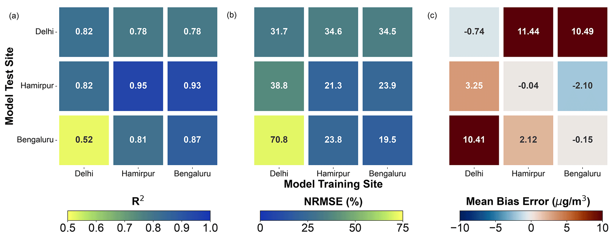
Figure 6 Assessment of the site-wise transferability of annual models. Performance evaluation metrics of Eqs. (2)–(4), with the training site on the x axis and the test site on the y axis. Metrics are the coefficient of determination (R²) (a), normalized root mean square error (NRMSE) (b), and mean bias error (MBE) (c). For each metric, the diagonal pattern of the best performance (from the upper left to the lower right) illustrates how calibration models perform best in the locations where they are trained. At each site, we compute the performance metrics by comparing the calibration model output to an independent test set that was held out from model training. This finding illustrates how regional differences in meteorology and aerosol composition can limit the transferability of calibration relationships. It is noteworthy that the calibration model trained in Delhi performed quite poorly in Bengaluru.

Applying the Delhi and Hamirpur models to the Bengaluru test dataset resulted in contrasting performance, with NRMSE values of 71 % and 24 % from the Delhi and Hamirpur models, respectively. It is likely the largely regional aerosol from Hamirpur has enough overlap in the speciation and mass concentration range with the Bengaluru aerosol that the models are somewhat interchangeable. This hypothesis is additionally evidenced by the overlap in coefficients from the theory-driven hygroscopic growth equations. Clearly, the differences in the composition of the Delhi and Bengaluru aerosols prevent an exchange between the models at these two sites, but there is enough preserved from the regional contribution to allow some support from the Hamirpur model to the Delhi data.

Some calibration efforts have sought a unified continental model for low-cost sensors by combining multiple reference and low-cost sensor pairs into one regression model (Barkjohn et al., 2021). Other studies have focused on interpolating between calibration sites to avoid washing out local effects, typically in a dense sensor network (Zheng et al., 2019). Our results show that although there are overarching similarities in model parameter selection, urban and rural environments are heterogeneous to the point of potentially barring a unified model. Additionally, seasonal variability within India necessitates at least monthly updates to the model coefficients.

4 Conclusions

We collocated low-cost sensors with reference grade PM_2.5 monitors in three environments in India, two urban (Delhi and Bengaluru) and one rural (Hamirpur), over the course of multiple seasons to characterize low-cost sensor performance across shifting emissions and meteorological regimes and develop calibration models. Internally, PA-II units demonstrated strong consistency, with low intra-sensor bias and high correlation. Relative to reference instruments, uncalibrated sensor performance varied diurnally and seasonally, with shifts being strongly associated with extreme mass concentrations, RH, and coarse-mode particles. The low-cost sensor signal generally overestimated mass concentrations relative to the reference instruments, which is a trend observed in the literature to be associated with hygroscopic growth (Jayaratne et al., 2018; Malings et al., 2019). We identified periods of low-cost sensor signal underestimation by a factor of 2–6× in the pre-monsoon period in Delhi and Hamirpur, when supramicron wind-blown dust particles are relatively abundant.

We demonstrated a relatively simple multilinear regression model, using only the low-cost sensor PM_2.5 signal, and a low-cost sensor RH could produce results that were well correlated (R² ≥ 0.8) with the reference signal at each site. These site-specific models provide the basis for a computationally efficient, well-constrained (NRMSE ≤ 25 %), and scalable calibration approach for low-cost sensing in India, despite the non-stationary and diverse aerosol dynamics of the region. Furthermore, we showed that our models can be transferred from site to site and still improve performance above the uncalibrated baseline, although a site-specific model generally has superior performance.

Our work also highlights a key caveat to low-cost sensor deployments and calibration in India, especially regarding long-term deployment. Models trained at a site with data from only one season may perform more accurately within that season than a seasonally balanced model but are unreliable at other times of the year. Based on our analysis, we hypothesize that it is better to use a model developed at a background site such as Hamirpur to correct data from an urban environment such as Delhi, since the composition of PM in Hamirpur represents a good subset of the variability in Delhi. On the other hand, since there are PM species only found in some urban environments in India, using models from these industrial microenvironments will less likely to produce accurate results outside of the training location. Our results showed that seasonality is especially important, given the contrast in meteorology and mass concentrations between the pre-monsoon and monsoon seasons. Although a multilinear regression approach produces well-constrained results, these models are not transferrable among seasons. Therefore, we advise future deployments to continuously operate a collocation site with at least one reference and low-cost sensor pair to evaluate calibration drift. Accounting for the temporal and spatial dynamics of aerosol characteristics will allow for the rapid scaling of low-cost sensors for communities in India to communities in need of transparent and accurate data.