the Creative Commons Attribution 4.0 License.
the Creative Commons Attribution 4.0 License.
 | 18 Oct 2023
Performance evaluation of MOMA (MOment MAtching) – a remote network calibration technique for PM2.5 and PM10 sensors
Lena Francesca Weissert
Geoff Steven Henshaw
David Edward Williams
Brandon Feenstra
Randy Lam
Ashley Collier-Oxandale
Vasileios Papapostolou
Andrea Polidori
We evaluate the potential of using a previously developed remote calibration framework we name MOMA (MOment MAtching) to improve the data quality in particulate matter (PM) sensors deployed in hierarchical networks. MOMA assumes that a network of reference instruments can be used as “proxies” to calibrate the sensors given that the probability distribution over time of the data at the proxy site is similar to that at a sensor site. We use the reference network to test the suitability of proxies selected based on distance versus proxies selected based on land use similarity. The performance of MOMA for PM sensors is tested with sensors co-located with reference instruments across three Southern Californian regions, representing a range of land uses, topography and meteorology, and calibrated against a distant proxy reference. We compare two calibration approaches: one where calibration parameters get calculated and applied at monthly intervals and one which uses a drift detection framework for calibration. We demonstrate that MOMA improves the accuracy of the data when compared against the co-located reference data. The improvement was more visible for PM10 and when using the drift detection approach. We also highlight that sensor drift was associated with variations in particle composition rather than instrumental factors, explaining the better performance of the drift detection approach if wind conditions and associated PM sources varied within a month.
- Article
(3194 KB) - Full-text XML
- Companion paper
-
Supplement
(921 KB) - BibTeX
- EndNote


Particulate matter (PM) is a major air pollutant with negative impacts on both the environment and human health (Kim et al., 2015; Anderson et al., 2012; Pope III, 2002; Rai, 2016). Smaller particles, known as PM2.5 (particles with an aerodynamic diameter < 2.5 µm), have the ability to penetrate deep into the lung and to cross into the blood stream and trigger inflammatory and mutagenic responses linked amongst other effects to cardiopulmonary disorders, diabetes and adverse birth outcomes (Feng et al., 2016). Coarse PM (PM10−2.5) tends to impact the upper respiratory tract and induce respiratory symptoms such as cough (Pope and Dockery, 1992). Short-term exposures to PM10 have been associated primarily with worsening of respiratory diseases, including asthma and chronic obstructive pulmonary disease (COPD) (California Air Resources Board, 2023). The spatial and temporal variability in PM is driven by multiple factors including anthropogenic PM emissions from traffic, construction and residential heating, which are main contributors to PM2.5, as well as natural sources such as mineral dust consisting mainly of particles in the coarse fraction (PM10−2.5) (Anderson et al., 2012; Atkinson et al., 2010). PM2.5 and PM10 are routinely measured by government and research organizations using reference-grade equipment that is either the filter-based Federal Reference Method (FRM) or continuous Federal Equivalent Method (FEM). However, reference monitoring networks are designed to measure regional air pollution to determine attainment of national ambient air quality standards and are often sparsely sited across a region due to high instrument and operational costs (Morawska et al., 2018; Snyder et al., 2013). The last decade has seen a rapid increase in the availability of PM sensors offering opportunities to measure PM with much denser networks and making them popular choices for citizen projects and community monitoring (Giordano et al., 2021; Liang, 2021; Snyder et al., 2013; Zimmerman, 2022).
Most PM sensors are optical sensors that utilize the light scattered by particles to determine the particle size and count which are then converted to particle mass based on assumptions about particle density, shape and refractive index. This poses a major challenge for calibrating PM sensors, as calibration factors may change with particulate type and composition, as well as meteorological conditions such as temperature or relative humidity (RH) which cause the particles to swell or shrink and change their light scattering (Badura et al., 2018; Morawska et al., 2018; Ouimette et al., 2022).
Thus, frequent field calibrations may be required if aerosol properties vary significantly over time (Liang, 2021; Johnson et al., 2018; Badura et al., 2018). While calibrations by co-location using regression analysis remain a popular choice, the costs and feasibility related to individual site visits and calibrations make them not a viable option for large and/or long-term sensor networks (Liang, 2021). Another approach is to apply a RH correction factor to account for the bias introduced due to high RH (Crilley et al., 2020; Liang, 2021). While this method has the advantage of being independent from the availability of reference data, it is not suitable for locations with consistently high RH and does not improve the accuracy as much as other calibration methods (Liang, 2021). Similarly, Barkjohn et al. (2021) developed a US nation-wide correction for PurpleAir sensors which is implemented in the AirNow Fire and Smoke Map (https://fire.airnow.gov/, last access: 5 October 2023). While the approach has intensively been tested for PurpleAir sensors, further research is required to evaluate its transferability to other sensor models (Barkjohn et al., 2021). Other studies have used machine learning (ML) approaches to train calibration models with enough co-location data to cover various meteorological and environmental conditions and make them more robust for long-term sensor deployments (Liang, 2021; De Vito et al., 2020; Loh and Choi, 2019). However, if conditions (e.g., different traffic conditions, different PM sources) at the co-location site are different from the conditions at the site of the final deployment, the model may no longer be suitable (De Vito et al., 2020; Liang, 2021). In addition, while being more robust and effective, ML may still suffer from challenges related to sensor degradation when sensors are deployed in a long-term fashion (Liang, 2021).
In previous publications, we demonstrated that a hierarchical network, consisting of well-maintained reference-grade instruments (referred to as “proxies”) and gas-phase (O3, NO2) sensors, can be used to correct sensors remotely (Miskell et al., 2018, 2019; Weissert et al., 2020). The correction framework, which we named MOMA for MOment MAtching, is based on the assumption that the probability distribution over time of measurements at a proxy site is similar to that of the sensor site (Miskell et al., 2018, 2019; Weissert et al., 2020). We have demonstrated that this approach is able to successfully correct for sensor drift without the need of co-location.
In this paper, we examine how this remote calibration methodology performs for PM sensors deployed in Southern California. The network was established between 2020 and 2022 to supplement the reference network and supports California Assembly Bill 617 community monitoring. The network is maintained by South Coast Air Quality Management District (AQMD) and covers three main regions, including the city of Los Angeles (LA), the Inland Empire (IE) and a desert region of Riverside County (RC Desert). These three regions differ in terms of land use, terrain and meteorology, offering an opportunity to test MOMA under different seasonal conditions and PM sources.
The network consists of over 60 sensors, for which the overhead for manual calibration would be prohibitive. Thus, using the MOMA approach, the sensors are calibrated at monthly intervals, and new calibration gains and offsets are uploaded to a cloud to provide real-time calibrated data which are displayed on the South Coast AQMD AQ Portal (https://aqportal.aqmd.gov/, last access: 5 October 2023). In order to validate the MOMA procedure applied across the network, the focus of this paper is on six sensors that are co-located with a reference instrument at air monitoring sites (AMSs). Here, we compare the monthly calibration approach to an automated drift detection approach to apply the calibration when drift between a sensor and the proxy site was detected using data from January to December 2021 (Miskell et al., 2018, 2019; Weissert et al., 2020).
A key part of MOMA is the identification of a suitable proxy site for each sensor in the sensor network. Previous work has shown that the nearest reference site is a suitable proxy to calibrate O3 concentrations, which are regionally well correlated (Miskell et al., 2018, 2019). For NO2, which is spatially and temporally more variable, land use similarity proved to be a good criterion to select appropriate proxy sites (Weissert et al., 2020). PM2.5 levels tend to be relatively homogeneous across an urban region, suggesting that the closest reference site could be a suitable proxy. However, PM10 can be spatially more variable due to the shorter lifetime and more variable sources, and a proxy selected based on distance may not be suitable (Pinto et al., 2004; Sardar, 2005). Thus, we also determine suitable proxies for calibrating PM2.5 and PM10.
2.1 Data
This study uses data from a network of Aeroqual AQY v1.0 (AQY) sensor systems from Aeroqual Ltd, Auckland, New Zealand. The AQY measures O3, NO2, PM2.5, PM10, temperature and relative humidity. A detailed description of the AQY sensor system is available in Weissert et al. (2020) and Miskell et al. (2019). The focus of this paper is the PM sensor (model SDS011, Nova Fitness Co., Ltd, Jinan, China) inside the AQY sensor system. The SDS011 is an optical light-scattering device which outputs PM2.5 and PM10 mass concentration (µg m−3) measurements. Previous studies of this sensor have shown a high PM2.5 correlation with reference instruments (Badura et al., 2018; Liu et al., 2019), but PM10 values may be underestimated (Budde et al., 2018; Kuula et al., 2020). Nevertheless, we use both PM2.5 and PM10 measurements to evaluate the performance of our network calibration technique applied to PM data. The SDS011 sensor was factory calibrated against a Met One 9722 eight-channel optical particle counter (Met One Instruments, Inc., Grants Pass, Oregon, USA) using 1 µm latex microspheres. The AQY performs a humidity correction using an algorithm based on the Köhler theory with an empirically derived scalar (Crilley et al., 2018). The AQY PM measurements were field and laboratory evaluated by South Coast AQMD's Air Quality Sensor Performance Evaluation Centre (AQ-SPEC) (http://www.aqmd.gov/aq-spec/sensordetail/aeroqual-aqy-v1.0, last access: 5 October 2023), showing strong correlations with the co-located FEM GRIMM data () and low to moderate intra-model variability.
We used data from six AQY sensors co-located at AMSs, referred to as “co-location sites” in this paper, equipped with a reference-grade instrument, which allowed us to test the performance of the remote calibration framework (Table 1). Reference data from the co-location AMSs were obtained either from AirNow (https://www.airnow.gov/, last access: 5 October 2023) or directly from South Coast AQMD. Refer to Table S1 in the Supplement for instrumentation at each site. The six AQY sensors were deployed between April 2020 and January 2021 (Table 1). While PM2.5 data were available since the start of the deployment, PM10 sensors were only activated at the start of January; thus we focus on data from January to December 2021 for the following analysis. Fog can frequently be present between October and February in the study area, driven by lower inversion levels (Qin et al., 2012; Witiw and LaDochy, 2008), and lead to overestimates of PM2.5 and PM10 (Budde et al., 2018) (Fig. S1 in the Supplement). We developed a fog alert, and data impacted by fog were removed from this analysis. This affected around 1 % of the data at each site and was mostly observed in November, December and February.
To get a better understanding about the composition of measured particles and how this impacts the performance of MOMA, we used speciation data collected at the Riverside–Rubidoux (RIVR) AMS. All speciation data were obtained using the RAQSAPI package (Mccrowey et al., 2021), which enables downloading monitoring data from the US Environmental Protection Agency's Air Quality System service. We focused on parameters representing crustal material, trace ions, secondary ions, elemental carbon (EC) and organic carbon (OC) and followed the classification described in Daher et al. (2013) (Table S2).
Surface meteorological data from Riverside Municipal Airport, situated ∼ 6 km south of the Riverside–Rubidoux AMS, were downloaded from the NOAA Integrated Surface Database (ISD) via the worldmet package in R (Carslaw, 2023).
Table 1Information about AQY sensors and their co-location sites, as well as deployment dates and data completeness (excluding fog data).
The statistical analysis was performed in R (v.4.1.3) using tidyverse (Wickham et al., 2019), lubridate (Grolemund and Wickham, 2011), zoo (Zeileis and Grothendieck, 2005), ggrepel (Slowikowski et al., 2023), openair (Carslaw and Ropkins, 2012), RAQSAPI (Mccrowey et al., 2021), ggplot2 (Wickham, 2016), dplyr (Wickham et al., 2022), ggmap (Kahle and Wickham, 2013) and ggpmisc (Aphalo, 2023).
2.2 Study area
This study was performed in Southern California in a region that is under the jurisdiction of the South Coast Air Quality Management District (SCAQMD). AQY sensors measuring PM were co-located at two AMSs in the city of LA (CELA, CMPT), two AMSs in the IE (RIVR, MLVB), and two AMSs in the RC Desert (INDIO, PALM) (Table 1). The LA region is representative of downtown LA, and PM levels are likely dominated by emissions from transport and other combustion processes (Oroumiyeh et al., 2022). The IE is situated in a predominantly rural and agricultural area about 80 km inland from downtown LA. It is situated downwind from LA for the majority of the year, which means that PM levels in the area will be influenced by the particulate matter coming from LA (Daher et al., 2013). Northeasterly Santa Ana Winds (SAWs) become more frequent during the autumn and winter months impacting PM levels in the IE. SAWs are associated with very dry air and good visibility in the absence of wildfires, as urban pollutants are blown offshore. However, they are also key drivers of large wildfires enabling them to spread faster and transporting smoke PM from inland areas to the more populated regions (Aguilera et al., 2020). The RC Desert region is located north of Salton Sea and surrounded by mountains. The region is drier and hotter compared to LA and the IE. The RC Desert experiences high levels of PM10, dominated by the coarse fraction, driven by erosion and increasing emissions from the drying Salton Sea (Ostro et al., 2000; Miao et al., 2022).
2.3 Remote network calibration
MOMA was developed for hierarchical air monitoring networks that consist of well-calibrated reference grade instruments acting as “proxies” which are used to calibrate the sensors deployed in the field. The technique is described in detail in Miskell et al. (2016, 2018, 2019). Here, we calibrated sensors co-located at the AMSs against a remote reference proxy. The performance of the calibration against the proxy was then evaluated by comparing the calibrated data against the co-located reference data using the metrics mean absolute error (MAE), root mean squared error (RMSE) and coefficient of determination (R2). We tested two approaches to calibrate the PM2.5 and PM10 sensors in this study.
Figure 1(a) PM2.5 and (b) PM10 South Coast AQMD reference air monitoring networks colored by different regions. The map was created using ggmap (Kahle and Wickham, 2013). Co-location sites are highlighted by black squares.
The first approach was a monthly MOMA calibration using the last 2 weeks of each month to select a calibration window of 7 consecutive days to calculate the calibration parameters which were then applied from the first to the last calendar day of the subsequent month. The last 2 weeks of the month were selected to ensure the most recent data were used to determine calibration gains and offsets. The calibration gains, , and offsets, , were calculated by matching the mean, E, and variance, var, of the sensor data, Y, at location i and proxy data, Z, at location k over the time interval as described in Miskell et al. (2018, 2019) and summarized in Eqs. (1) and (2).
A calibration window was considered suitable if the data completeness for both proxy and sensor was greater than 85 % and the temporal variation in the sensor and proxy reference data was similar (i.e., there was no evidence of local effects that were only present at the sensor site or proxy site). We also avoided periods when we detected fog using Aeroqual's fog detection algorithm.
The second approach used a previously described drift detection framework (Miskell et al., 2016) to trigger a MOMA calibration. The drift detection framework uses three statistical tests to detect sensor drift: a two-sample Kolmogorov–Smirnov (K-S) test (K-S test p value) and a mean-variance (MV) moment-matching test for the slope, , and the intercept, . The statistical tests were calculated over a 3 d running averaging window, td, and an alarm was triggered when any of the tests exceeded the predetermined threshold, tf, for a period of 5 consecutive days. These periods were selected to limit short-term fluctuations due to local effects but to capture the regional effects, which is ensuring that diurnal and regional variations dominate (Miskell et al., 2018, 2019). The following thresholds were used to determine if a sensor drifted: K-S test p value < 0.05 (the two distributions are significantly different); 0.75 < > 1.25; −5 µg m−3 > > 5 µg m−3. These thresholds may be adjusted to be more or less sensitive to differences between the sensor and the proxy data. While adjusting all parameters and alarm triggers exceeded the scope of this study, preliminary analysis using data from “RIVR coloc”, “MLVB coloc” and “CELA coloc” showed that a shorter 4 d window, tf, may be more suitable for the AQY sensors located in the IE but not the city of LA. This framework was applied to the six AQY sensors co-located at the AMSs (Table 1) using data from January to December 2021.
2.4 Proxy selection
We compare proxies selected based on distance to proxies with similar land use. Land use variables used for the analysis were (a) road length (motorway, primary roads) within a 1 km buffer around the site, (b) distance of the site from a motorway and (c) elevation. These are simple and widely available and have also been identified as good predictors for PM in land use regression studies in the USA (Kloog et al., 2012; Lee et al., 2016) and Europe (Eeftens et al., 2012). To select proxy sites with the most similar land use we used a supervised classification technique, the k-nearest neighbor classification (kNN), as described in more detail in Weissert et al. (2020).
Data from the reference network were used to identify suitable proxies, which had two main advantages over using sensor data. First, the availability of long-term reference data allowed testing and developing suitable criteria for proxy selection without relying on sensor data, which are often not available until deployed in the field. Second, we eliminated any uncertainties associated with sensor performance, such as sensor drift.
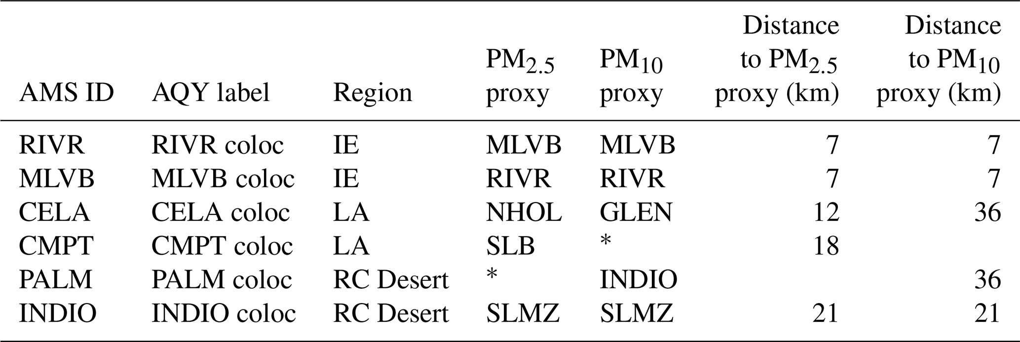
Figure 1 shows the network of reference PM2.5 and PM10 monitors managed by SCAQMD. Sites with co-located AQY sensors, including Los Angeles, N. Main Street (CELA), Compton (CMPT), Mira Loma–Van Buren (MLVB) and Rubidoux (RIVR), were used as test locations for which a suitable PM2.5 proxy is found. As SLMZ was the only available PM2.5 proxy site for Indio–29 Palms (INDIO), this site was not included in the proxy selection analysis for PM2.5. CELA, MLVB, RIVR, Palm Springs (PALM) and INDIO were used as test locations to identify suitable for PM10 proxies (Fig. 1).
To evaluate the similarity between data at a proxy site and data at a test location we calculated the MAE, R2 and the two-sample K-S test statistic for each possible proxy and co-located test location based on daily averaged reference data. The K-S test statistic is a measure of the maximum distance between two cumulative distributions and was used to compare the cumulative distribution of the proxy reference data to that of the reference at the co-located test location. An ideal proxy should exhibit a low MAE and K-S test statistic, as well as a high R2 value.
Figure 2PM2.5 and PM10 reference time series for a 7 d period grouped by regions (i.e., IE, LA, RC Desert). Co-location test sites are the solid lines. Sites with dashed lines are proxy sites only.
3.1 General characteristics of the data
PM2.5 levels seem to be comparable across the sites and regions in LA and the IE, but lower levels were observed in the RC Desert (Fig. S2). There are also distinct differences in the PM10 concentrations with higher levels observed in the IE (RIVR, MLVB). PM2.5 concentrations were highest in autumn and generally more variable over the autumn and/or winter period. The time series shown in Fig. 2 show that while short-term local effects are visible (particularly for PM10 in the IE and RC Desert), overall diurnal PM2.5 and PM10 variations across sites within the same region were similar. This suggests that MOMA could be an effective calibration framework for PM, since the underlying requirement, that the diurnal patterns of pollutants at the proxy site and at the site to be calibrated are similar, seems to be met, particularly for PM2.5. For PM10, a more careful selection of a suitable calibration window may be required, given the short-term local differences.
Table 2Table of the site names associated with the AMS IDs used in Fig. 1.
3.2 Proxy selection criteria
Figure 3 shows the MAE, R2 and K-S test statistic for proxies located at various distances away from the four (PM2.5) and five (PM10) co-located AMS test locations. The figure demonstrates whether data obtained from the nearest site or the site with the most similar land use closely resemble the data at the respective test location. The figure illustrates that in most cases the nearest proxy site rather than the site with the most similar land proves to be the most appropriate proxy, resulting in the lowest MAE and the highest R2 throughout the entire year. Using the K-S test statistic as a measure of similarity across probability distributions reveals a slightly different pattern, suggesting that PM2.5 CMPT or SLB may be more suitable proxies for CELA and that PM2.5 CELA could be a suitable proxy for MLVB or RIVR when upwind from MLVB or RIVR.
However, there are exceptions to this observation, suggesting that other factors, such as PM sources associated with the surrounding land use, terrain or prevailing wind direction, likely also contribute to the suitability of a proxy. For example, a proxy further away (CELA) seems to perform similarly to a nearby proxy (UPL) for PM2.5 at Mira Loma (MLVB). Mira Loma is downwind from CELA for most of the year, possibly explaining the low MAE against MLVB. The CRES site also seems to be a poorer PM2.5 proxy for MLVB and RIVR, which may be due to its location at higher altitudes, as well as being separated from MLVB and RIVR by the San Bernardino mountains (> 1200 m high). Nevertheless, the nearest proxy generally resulted in the most similar distribution with the lowest K-S test statistic, as well the lowest MAE and highest R2. Thus, we suggest selecting PM proxies based on distance for the following analysis, as well as future deployments, as long as the nearest proxy is within the same airshed (e.g., not separated by mountains).
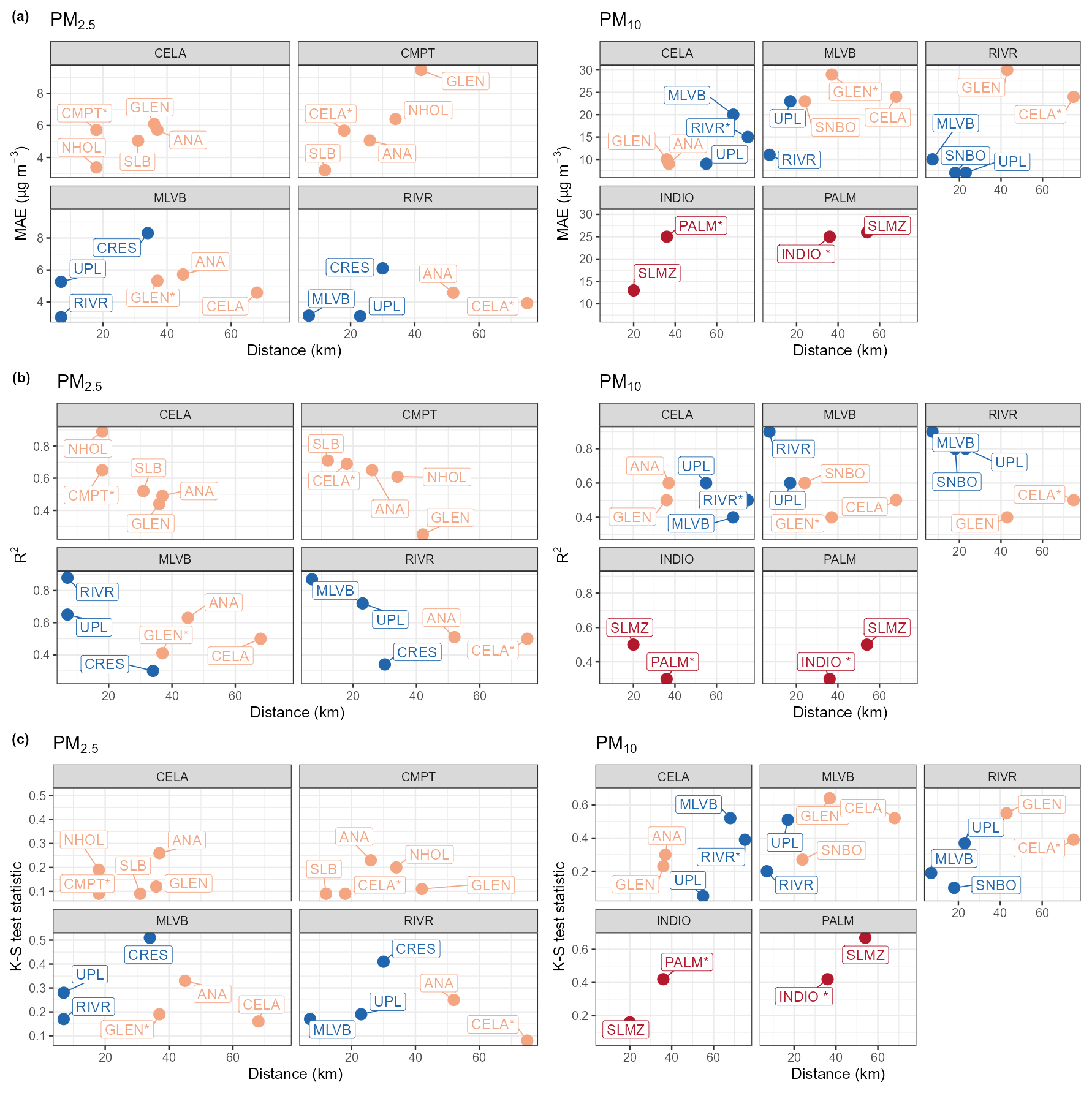
Figure 3(a) MAE, (b) R2 and (c) K-S test statistic colored by region (LA: orange; IE: blue; RC Desert: red) for different proxies against distance to the co-located test location for PM2.5 (CELA, CMPT, MLVB, RIVR) and PM10 (CELA, MLVB, RIVR, INDIO, PALM). The site with the most similar land use to the test site is labeled with a “*”. The proxy site is labeled in each panel. The full site names are shown in Table 2. An ideal proxy would have a low MAE and K-S test statistic, as well as a high R2 value. Proxies on the left hand side are closest to the co-located test location and therefore representative of the nearest proxies.
3.3 MOMA calibration performance
The performance of MOMA was evaluated using sensors that were co-located at an AMS. Each sensor was mapped to its nearest proxy (Table 3), calibrated using the MOMA technique and compared to its co-located South Coast AQMD AMS using the metrics MAE, RMSE and R2.
Table 3List of AQY sensors co-located at South Coast AQMD AMS sites with their proxy reference sites.
∗ There are no PM10 data available from CMPT and no PM2.5 measurements available from PALM.
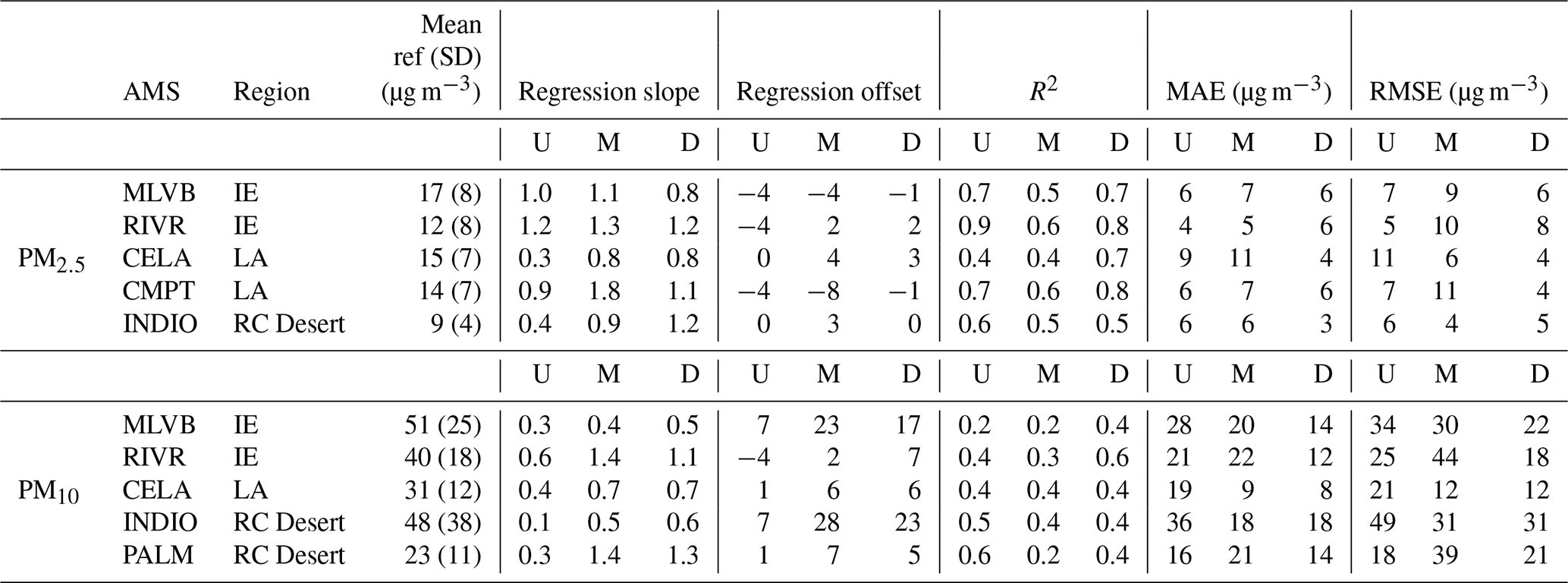
Table 4The 24 h averaged PM2.5 and PM10 summary statistics for the AQY sensors against the co-located reference before the calibration (U), after the monthly calibration (M) and the drift calibration (D) over the 12-month period from January 2021 to December 2021.
3.3.1 PM2.5
Table 4 shows the 24 h averaged PM2.5 and PM10 summary statistics for the AQY sensors against the co-located reference before the calibration (gain = 1, offset = 0 + RH correction) (U), after the monthly calibration (M) and the drift calibration (D) over the 12-month period from January 2021 to December 2021. The monthly MAEs are shown in Fig. 4.
The sensors in the LA and the RC Desert regions were under-reading PM2.5 concentrations prior to calibration; this was particularly evident for the AQY co-located at the INDIO AMS (slope: 0.4). These sensors show a clear improvement with both the monthly and drift calibration applied as indicated by a slope closer to 1 and an up to 60 % reduction in the MAE and RMSE, although the improvement varies across the sensors (Table 4). The monthly and drift calibrations did not improve the R2 or slope for the sensors in the IE at MLVB and RIVR. Unlike the AQY sensors in the LA region or the RC Desert the uncalibrated data showed a strong correlation with the co-located reference, R2 (0.7/0.9), and the slope (1.0/1.2) and MAE (4–6 µg m−3) were already within the range of calibrated slopes and MAE. This suggests that the standard factory sensor calibration transferred well to the field at MLVB and RIVR. Calibrating the sensor data against the proxy, however, seems to have introduced errors. There are several reasons for this. Firstly, Fig. 4 shows that the MAE between the co-located reference data and the proxy data is larger at RIVR then the MAE for the uncalibrated data against the co-located reference data, indicating that the MLVB proxy was not always suitable for MOMA calibration of the RIVR sensor. This is also supported by the differing probability distributions from the two sites (Fig. S3), which suggests the sites were exposed to different PM levels. On the other hand, the probability distributions for CELA and NHOL PM2.5 data and those for CMPT and SLB were very similar (Fig. S3), and hence the MOMA calibration process produced improved accuracy.
Secondly, monthly variability in particle source and composition will impact the reliability of the MOMA calibrations particularly for those performed at monthly intervals. For example, the very high monthly MOMA MAE for February at CELA, MLVB and RIVR suggests the January particle composition was not representative of that observed in February at these sites. Particle composition is known to vary with different wind directions (desert versus marine and urban particles) and impact the sensor reading as observed in previous studies (Castell et al., 2017; Gao et al., 2015; Giordano et al., 2021; Kelly et al., 2017). The effect of this phenomenon is particularly visible between November and February when wind was more variable. This is supported by Fig. 4, which shows that for both the LA and IE regions the MAE tended to be higher in November–December and January for both uncalibrated and calibrated data. The difference between the proxy and the co-located reference data also tended to be larger during these months.
A similar month-to-month variability in the MAE can be observed when comparing the reference monitor (BAM-1020, Met One Instruments, Inc., Grants Pass, Oregon, USA) at RIVR against the reference grade optical instruments – T640 (Teledyne API, San Diego, USA) and the GRIMM optical particle counter (EDM 180, GRIMM Aerosol Technik GmbH and Co., Airing, Germany) – also located at the RIVR site. The T640 and GRIMM are both optical particle counter instruments that determine the aerosol particle size distribution from which they estimate the PM concentration. The BAM-1020 samples aerosols through a PM10 inlet and uses a very sharp cut cyclone (VSCC) to classify it into PM2.5 before collecting it on a filter tape and determining the PM2.5 concentration by the aerosol's attenuation of a C14 beta radiation source (Hagler et al., 2022). Due to the differences in the measurement principles, the instruments can give different results depending on the properties of the measured particles.
The T640 and GRIMM match each other consistently across the year (similar technologies), but the BAM and T640 MAE and the BAM and GRIMM MAE were higher in general and highest during the November and December months. This further shows how differences between measurement technologies will be exacerbated when particle composition is variable. This is discussed in more detail in Sect. 3.5.
Thirdly, measurement noise in the hourly reference data from the beta attenuation monitors deployed at the sites may be too high to reliably calibrate low-cost sensors when concentrations are low (< 40 µ g m−3) as often was the case in the RC Desert (Hagler et al., 2022; Johnson et al., 2018; Zheng et al., 2018). The calibration improved the data most during the summer months with the MAE equal or below 5 µg m−3.
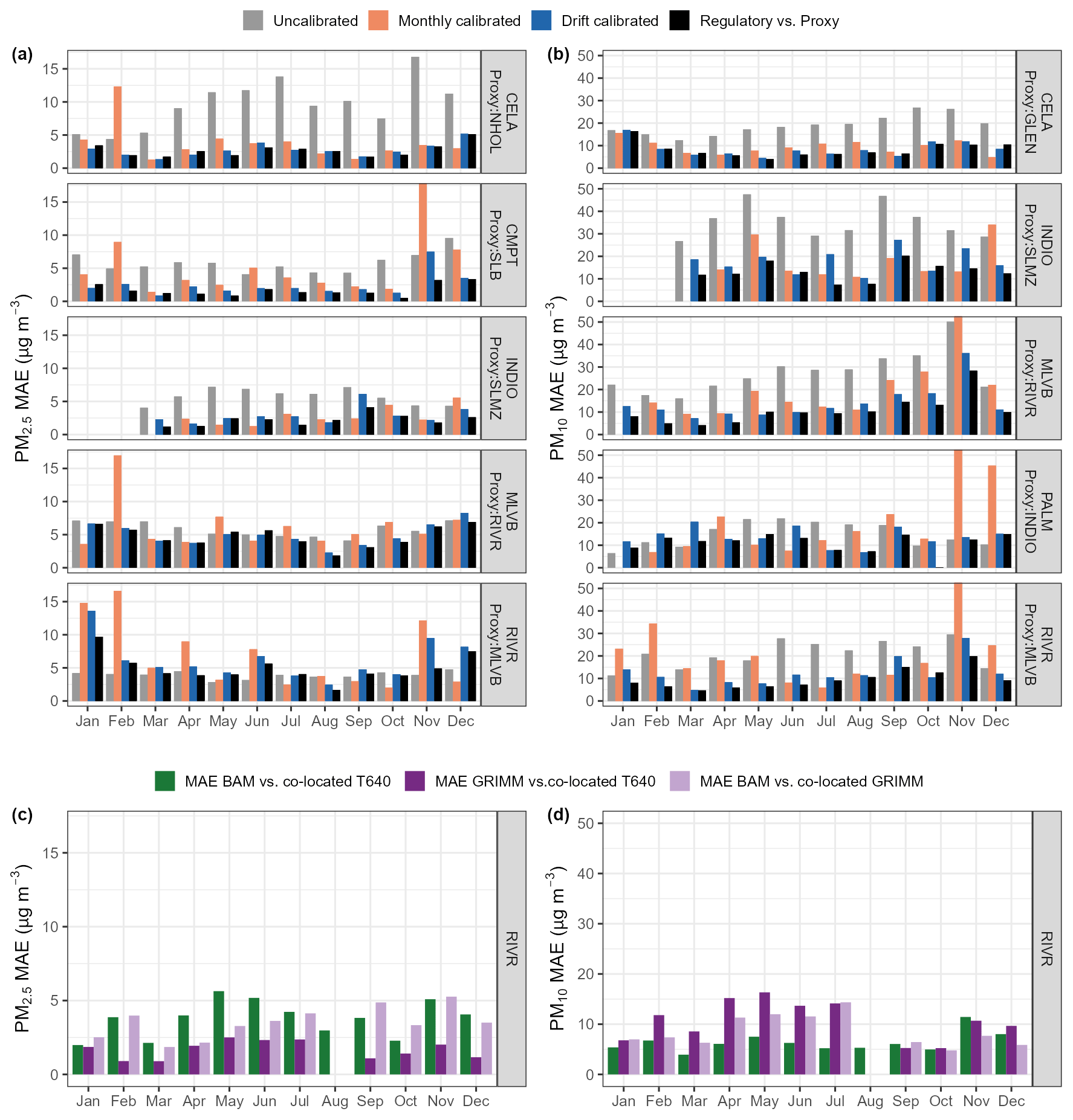
Figure 4Bar charts showing the uncalibrated (gain = 1, offset = 0 + RH correction), monthly-calibrated and drift-calibrated MAE between the AQY 24 h averaged PM2.5 (a) and PM10 (b), and the co-located reference. For comparison it also shows the MAE between the proxy reference and the co-located reference in black. Panels (c) and (d) show the MAE between the 24 h averaged BAM and co-located T640, the GRIMM and the co-located T640, and the BAM and the co-located GRIMM.
3.3.2 PM10
As expected, the PM10 data from the sensors generally showed a poorer agreement with the co-located reference with a high MAE (16–36 µg m−3) and RMSE (18–49 µg m−3) and low R2 (0.2–0.6) (Table 4) for uncalibrated data. The uncalibrated data were also underestimating PM10 concentrations, particularly in the RC Desert (INDIO, PALM) as shown by the low slope (0.1–0.3). This is in agreement with previous work which showed that the SDS011 underestimates PM10, particularly for particles greater than 5 µm which dominate in the RC Desert (Budde et al., 2018; Kuula et al., 2020; Ostro et al., 2000).
The monthly and drift-triggered MOMA calibrations had a clear positive impact on PM10 and improved the accuracy, as indicated by a nearly 60 % decrease in the MAE and a 40 % decrease in the RMSE in the LA region (CELA) (Table 4). However, the scatter remained and resulted in no improvement in the R2. The drift detection framework also improved the accuracy of the data at the two AQY sensors located in the IE. The monthly calibrations, on the other hand, decreased the accuracy at RIVR where the MAE and RMSE were higher after the calibration compared to uncalibrated data (Table 4).
The proxy and REF MAE (Fig. 4) was highest in the RC Desert suggesting that SLMZ is not a suitable proxy for PM10 at INDIO. To some extent this is expected since the PM coarse fraction (PM10–PM2.5) is more dominated by local sources than PM2.5 (Pinto et al., 2004).
However, similar to PM2.5, there was month-to-month variability in the calibration performance, with better improvements during summer and poor performance in November, particularly in the IE and RC Desert (Fig. 4). Potential factors that contribute to the high MAE in November are further discussed in Sect. 3.5.
A comparison of the PM10 data from the reference instruments at RIVR (BAM, GRIMM, T640) shows that the MAE across different instrument types can be as high as ∼ 15 µg m−3, and the GRIMM and T640 PM10 MAE is the highest – the opposite of the PM2.5 result. This observation illustrates the importance of the assumptions used to relate signal to aerodynamic radius and mass, which are different for different instrument types.
3.4 Drift detection triggers
The results from the drift detection framework tests are shown in Fig. 5 (K-S test p value; MV slope test, ; and the MV intercept test, for PM2.5, and PM10 measured by a PM sensor deployed in the LA region and one in the IE region. The black points indicate when the framework triggered a drift alarm and calibration. It is evident that most alarms were raised due to significant differences in the probability distributions (K-S test p value < 0.05), followed by a change in the slope between the proxy and sensor (MV slope test). Alarms triggered by the K-S test are spread across the whole year but are generally more common during the summer months; concentrations are possibly lower then, so instrument noise becomes important and is determining the signal distribution across the observed range. In the IE (RIVR) alarms related to changes in the MV slope were clustered around February, May and September–October suggesting more frequent changes in environmental conditions (e.g., RH) or particle composition and size during these months (discussed in Sect. 3.5). The AQY sensor installed at the CELA AMS sent off alarms that were more spread across the whole year, suggesting that sensor drift at this site was not related to seasons. The figure also shows that there are frequent calibrations within a month at both sites likely due to within-month changes in meteorological and environmental conditions (discussed in Sect. 3.5). This partly explains the better performance of the drift-calibrated data compared to the monthly calibrated data.
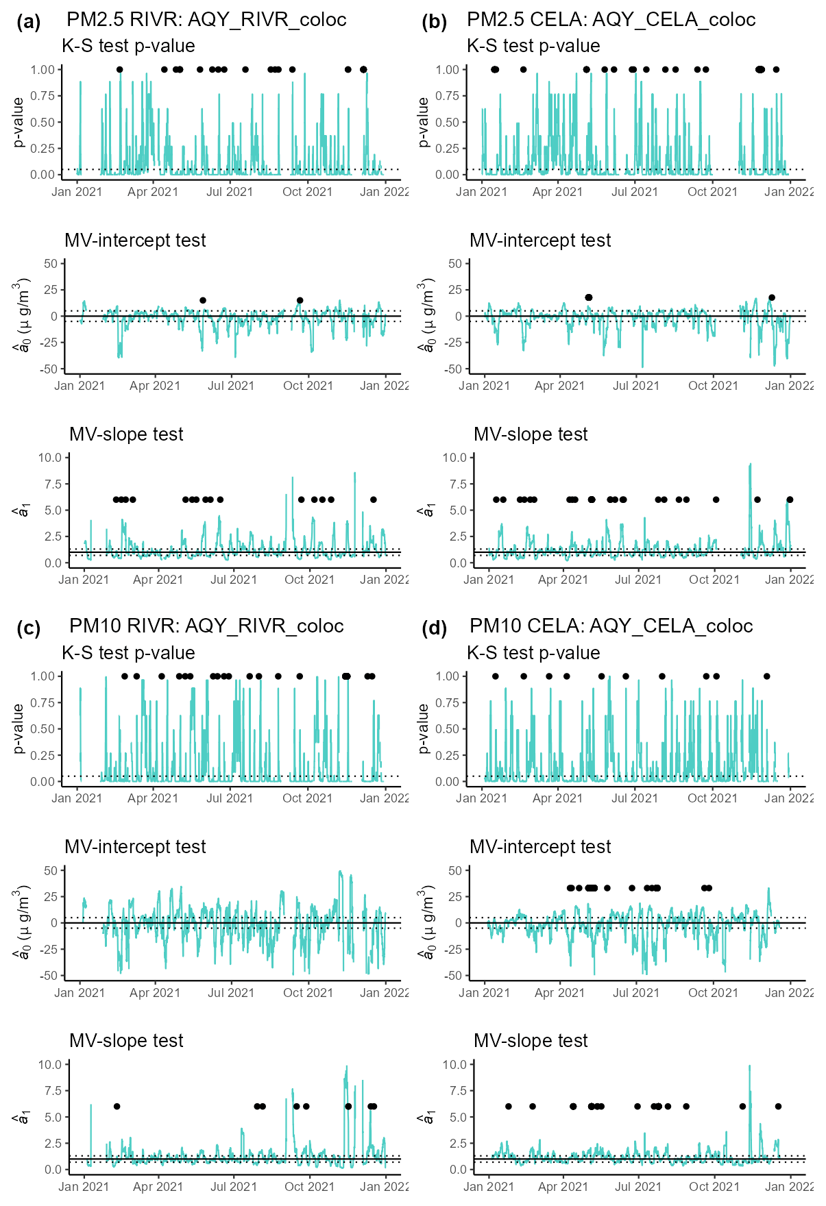
Figure 5Test statistics from drift detection framework for a site in the IE region (a, c) and one in the city of LA region (b, d) for PM2.5 (a, b) and PM10 (c, d). The black points show when the drift detection framework resulted in an alarm and triggered a calibration. The dotted lines represent the thresholds used to trigger a drift alarm: K-S test p value < 0.05; −5 µg m−3 > > 5 µg m−3; 0.75 > > 1.25. A drift alarm (black dot) was triggered when thresholds were exceeded for 5 consecutive days.
Figure 6 shows the temporal variability in monthly and drift-calculated gains for sensors in the IE, LA and RC Desert regions. The temporal variation in the PM2.5 and PM10 gains calculated by the monthly calibrations (Fig. 6b and d) show a distinct seasonal pattern with higher gains (∼ 2–3) during autumn and winter and lower gains (∼ 1) during the summer months, particularly in the IE region. An opposite pattern is visible in the RC Desert where gains were not only reaching a maximum over the summer months but were also around 6 times higher than those in the IE or LA regions. The gains from the drift detection framework were more variable, as visible from the more frequent step changes, but also showed some seasonal dependence. These results suggest that unlike calibrating for sensor drift (which would be shown as a continuous increase in the slope over time as observed when calibrating O3 sensors; Miskell et al., 2019) PM sensors are calibrated for different conditions, which can vary frequently as shown by the step changes in the drift gains.
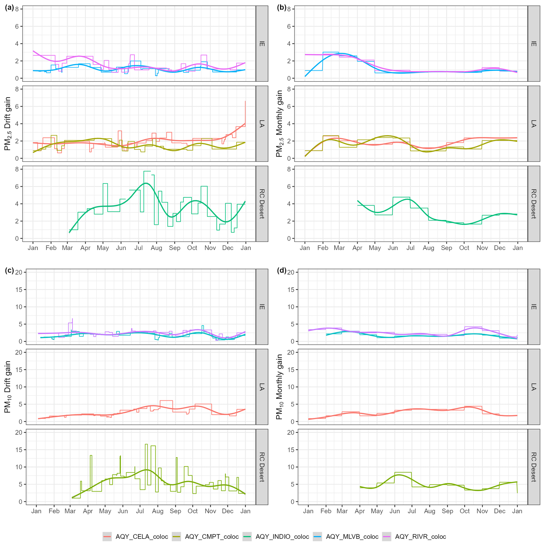
Figure 6Temporal variation in the gains as calculated from the drift detection framework (a, c) and the monthly calibrations (b, d) for PM2.5 (a, b) and PM10 (c, d). Step changes refer to a change in the calibration gain, and a smooth curve was fitted through the data points to visualize the overall temporal trend of the gains.
3.5 Particle composition variability
As observed in the previous sections, calibrating PM sensors can be challenging in complex areas where particle composition, size and physical properties (i.e., shape and refractive index) vary spatially and temporally (Kuula et al., 2020). In this section, we discuss some of the origins for the variations in particle composition with a specific focus on the Riverside area (RIVR AMS).
The wind data from Riverside Municipal Airport, shown in Fig. 7, clearly indicate the seasonal variation in the wind direction with north and northeast winds dominating during the late autumn–winter months and west winds dominating during the rest of the year. It is also visible that wind is more variable in late autumn and winter, possibly explaining the more frequent alarms observed for these months at Riverside (Fig. 5). The north and northeast winds correspond to the SAWs which are associated with very dry downslope airflow from the northeast and common between October and April, with a peak in December and January (Aguilera et al., 2020). Typically, PM concentrations during SAW conditions are dominated by coarse particles of crustal components (Guazzotti et al., 2001; Qin et al., 2012).
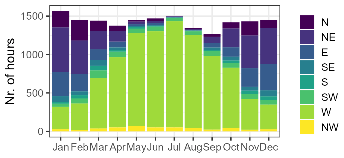
Figure 7Number of hours dominated by different wind direction measured at Riverside Municipal Airport during each month.
This is in agreement with observations from Fig. 8 which shows higher concentrations of crustal material and elemental carbon during north, northeast and northwest winds, reaching a maximum in November. Organic carbon concentrations, likely driven by traffic emissions, are similar across the dominant wind directions with maximum concentrations observed in November. Higher autumn and winter OC concentrations have previously also been observed by Daher et al. (2013) and were explained by stronger atmospheric stability which restricted atmospheric mixing. Higher concentrations of OC observed over the summer months when EC concentrations were low are likely due to increased PM advection and secondary organic aerosol formation as commonly observed for the inland locations downwind from urban sites (Daher et al., 2013). Trace ions (chloride, sodium and potassium) and secondary ions (nitrate, sulfate and ammonium), on the other hand, are highest downwind from the city of LA, reaching a maximum in spring–summer due to increased photochemical activity and a larger contribution of sulfate sources and its precursor (fuel and ship emissions) upwind of the city of LA (Daher et al., 2013).
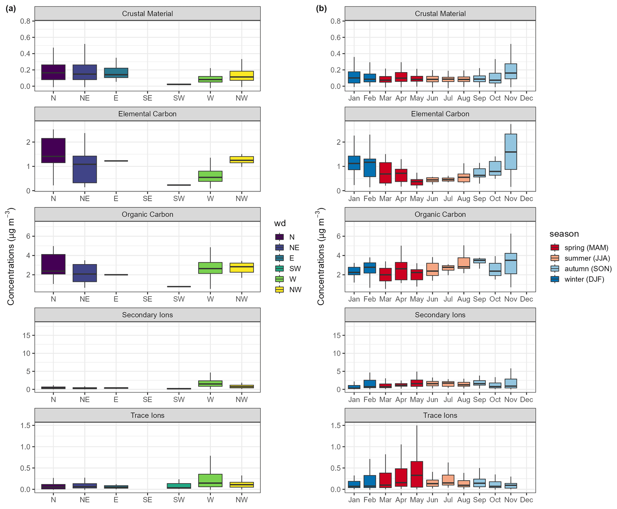
Figure 8Boxplots showing speciation concentrations collected at the Rubidoux (RIVR) AMS grouped into five categories (panels) plotted against wind direction (wd) (a) and for each month of the year colored by different seasons (b). Note that there were no data for southeast winds which were not common during the study period. The lower and upper hinges represent the 25th and 75th percentiles with the median marked inside the box. The lower and upper whiskers extend 1.5 × the inter-quartile range from the hinge.
Figure 9 illustrates the relationship between the BAM and co-located sensor data colored by wind direction and course fraction (1 – PM2.5/PM10). The figure reveals a clear slope dependence on the wind direction (< 1 when wind was from a northeast origin and ≥ 1 when wind from a western origin dominated), suggesting that it underestimates PM2.5 levels during northeastern wind (SAW conditions). These conditions correspond to a higher proportion of coarse fraction, likely associated with crustal material, further highlighting that the AQY is underestimating larger particles (Fig. 9b). In fact, Budde et al. (2018) found that the SDS011 used in this study strongly underestimates particles > 2 µm in the PM2.5 measurement.
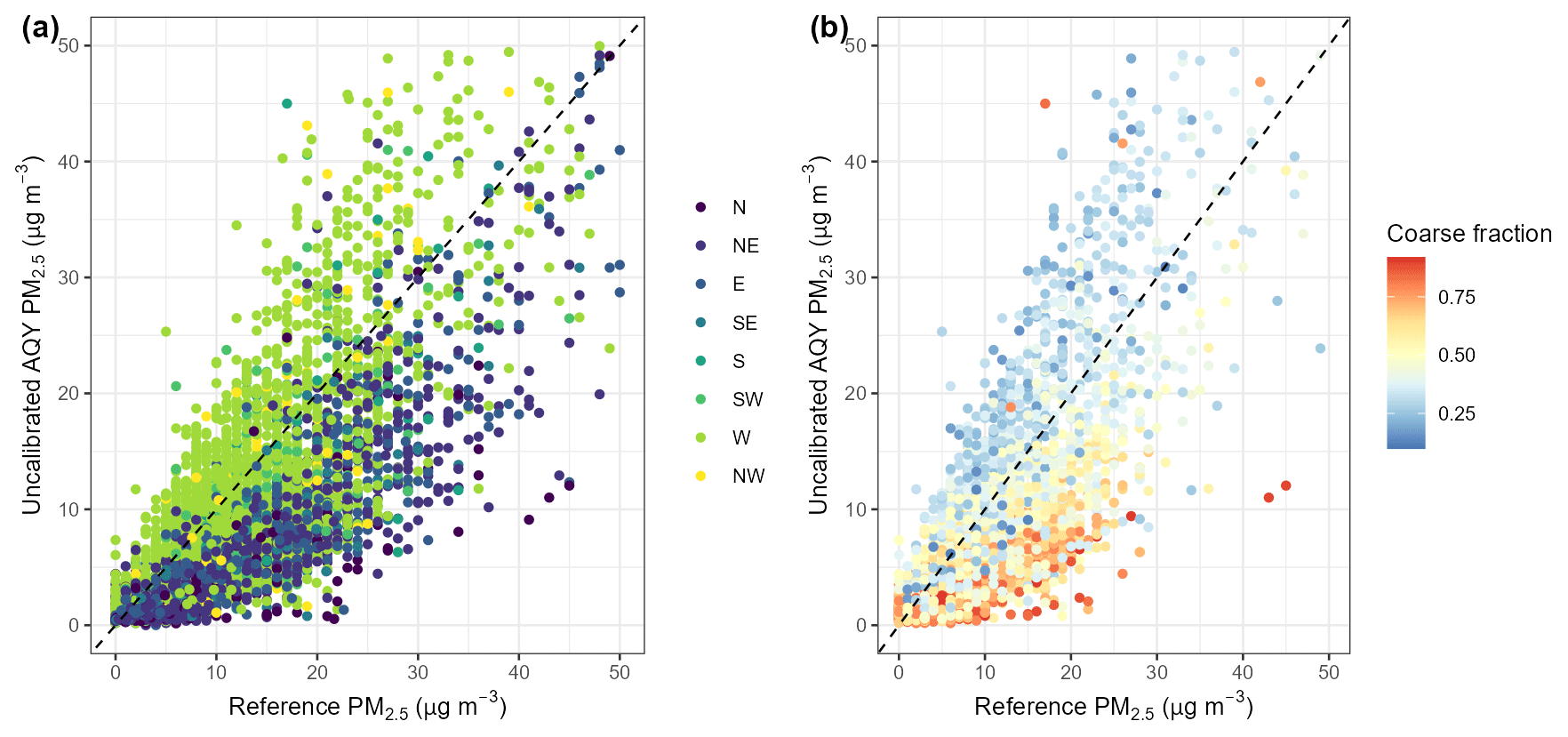
Figure 9Hourly uncalibrated low-cost sensor data against hourly co-located reference data at the Rubidoux (RIVR) AMS during 2021, (a) colored by wind direction and (b) colored by the AQY PM coarse fraction: 1 – PM2.5/PM10.
This work is part of a large study that set out to determine if a remote calibration framework (MOMA), previously developed for the correction of drift in O3 and NO2 sensors (Miskell et al., 2018, 2019; Weissert et al., 2020), can be applied for PM2.5 and PM10 data from PM sensors. We identified suitable reference proxies based on distance and presented two approaches to remotely calibrate data from sensor networks: (1) at monthly intervals and (2) using a drift detection framework that triggers a calibration when drift is detected. Our results show that averaged across all seasons and sites MOMA reduces the PM2.5 RMSE from 8 to 5 µg m−3 with average PM2.5 concentrations of 13 µg m−3. This is comparable to the improvement achieved from a global correction applied to PurpleAir sensors where the 24 h averaged PM2.5 RMSE was reduced from 8 to 3 µg m−3 (average PM2.5 reference concentration: 9 µg m−3) (Barkjohn et al., 2021). While both the monthly and drift calibration improved the accuracy of the data on average, the drift correction framework performed better. Overall, the improvement due to the MOMA calibration was more obvious for PM10 with an overall reduction in the RMSE from 30 to 21 µg m−3 at average PM10 reference concentrations of 39 µg m−3.
We note that calibrating PM sensors is more challenging than calibrating gas sensors (e.g., O3 in Miskell et al., 2019, and NO2 in Weissert et al., 2020) due to the spatial and temporal variations in particle composition and the resulting differences in response between the reference BAM instruments and the PM sensors. This was visible in the IE where particle composition varied between desert dust (north and northeast) and marine and urban aerosol (west) during the winter months, meaning that the monthly calibration applied may not be correct and data should be interpreted with caution. This also highlights that a more flexible proxy selection approach depending on dominant wind direction and particle source may be more suitable than using the same proxy site across all seasons.
Since the optical PM sensor accuracy depends on the atmospheric aerosol composition, it is expected that MOMA with the drift detection framework has an advantage over other methods such as calibration by co-location or using a mobile reference in that it is continuous, whereas the other methods are performed at discrete time periods and do not account for aerosol composition changes between calibrations. Future work will focus on optimizing MOMA and apply it to other PM sensors (e.g., PurpleAir sensors) (Collier-Oxandale et al., 2023).
The 10 min, 1 h and 24 h averaged data from the SCAQMD sensor network can be exported from https://aqportal.aqmd.gov/ (South Coast AQMD, 2023). The code is not publicly accessible due to intellectual property.
The supplement related to this article is available online at: https://doi.org/10.5194/amt-16-4709-2023-supplement.
GSH, DEW and VP formulated the overarching research goals and aims. DEW, LFW and GSH developed the methodology. BF, AC-O and RL managed and maintained the sensor network. LFW developed the software, performed the data analysis and prepared the manuscript with contributions from all co-authors. VP, AP and GSH supervised the project.
The authors declare the following financial interests/personal relationships which may be considered potential competing interests: Lena Francesca Weissert and Geoff Steven Henshaw are employees of Aeroqual Ltd, manufacturer of the sensor nodes used in these studies, and Geoff Steven Henshaw and David Edward Williams are founders and shareholders in Aeroqual Ltd.
Publisher's note: Copernicus Publications remains neutral with regard to jurisdictional claims in published maps and institutional affiliations.
The authors would like to acknowledge the work of the South Coast AQMD Atmospheric Measurements group of dedicated instrument specialists that operate, maintain, calibrate and repair air monitoring instrumentation to produce regulatory-grade air monitoring data. Additional appreciation is extended to the South Coast AQMD Laboratory for their work on the SASS PM speciation data that were accessed through the RAQSAPI R package.
This paper was edited by Albert Presto and reviewed by two anonymous referees.
Aguilera, R., Gershunov, A., Ilango, S. D., Guzman-Morales, J., and Benmarhnia, T.: Santa Ana Winds of Southern California Impact PM2.5 With and Without Smoke From Wildfires, GeoHealth, 4, 1–9, https://doi.org/10.1029/2019GH000225, 2020.
Anderson, J. O., Thundiyil, J. G., and Stolbach, A.: Clearing the Air: A Review of the Effects of Particulate Matter Air Pollution on Human Health, J. Med. Toxicol., 8, 166–175, https://doi.org/10.1007/s13181-011-0203-1, 2012.
Aphalo, P. J.: ggpmisc: Miscellaneous Extensions to “ggplot2”, https://CRAN.R-project.org/package=ggpmisc (last access: 16 October 2023), 2023.
Atkinson, R. W., Fuller, G. W., Anderson, H. R., Harrison, R. M., and Armstrong, B.: Urban Ambient Particle Metrics and Health: A Time-series Analysis, Epidemiology, 21, 501–511, https://doi.org/10.1097/EDE.0b013e3181debc88, 2010.
Badura, M., Batog, P., Drzeniecka-Osiadacz, A., and Modzel, P.: Evaluation of Low-Cost Sensors for Ambient PM 2.5 Monitoring, J. Sens., 2018, 1–16, https://doi.org/10.1155/2018/5096540, 2018.
Barkjohn, K. K., Gantt, B., and Clements, A. L.: Development and application of a United States-wide correction for PM2.5 data collected with the PurpleAir sensor, Atmos. Meas. Tech., 14, 4617–4637, https://doi.org/10.5194/amt-14-4617-2021, 2021.
Budde, M., Schwarz, A. D., Mueller, T., Laquai, B., Streibl, N., Schindler, G., Koepke, M., Riedel, T., Dittler, A., and Beigl, M.: Potential and Limitations of the Low-Cost SDS011 Particle Sensor for Monitoring Urban Air Quality, ProScience, in: ProScience, 3rd International Conference on Atmospheric Dust – DUST2018, 6–12, https://doi.org/10.14644/dust.2018.002, 2018.
California Air Resources Board: Inhalable Particulate Matter and Health (PM2.5 and PM10), https://ww2.arb.ca.gov/resources/inhalable-particulate-matter-and-health (last access: 31 July 2023), 2023.
Carslaw, D.: worldmet: Import Surface Meteorological Data from NOAA Integrated Surface Database (ISD), https://CRAN.R-project.org/package=worldmet (last access: 16 October 2023), 2023.
Carslaw, D. and Ropkins, K.: openair – an R package for air quality data analysis, Environ. Modell. Soft., 27–28, 52–61, https://doi.org/10.1016/j.envsoft.2011.09.008, 2012.
Castell, N., Dauge, F. R., Schneider, P., Vogt, M., Lerner, U., Fishbain, B., Broday, D., and Bartonova, A.: Can commercial low-cost sensor platforms contribute to air quality monitoring and exposure estimates?, Environ. Int., 99, 293–302, https://doi.org/10.1016/j.envint.2016.12.007, 2017.
Collier-Oxandale, A., Feenstra, B., Lam, R., Mui, W., Weissert, L. F., Henshaw, G. S., Papapostolou, V., and Polidori, A.: Applying the MOMA Remote Calibration Technique to PurpleAir PM2.5 Data to Improve Data Quality for a Large-Scale Sensor Network, to be submitted, 2023.
Crilley, L. R., Shaw, M., Pound, R., Kramer, L. J., Price, R., Young, S., Lewis, A. C., and Pope, F. D.: Evaluation of a low-cost optical particle counter (Alphasense OPC-N2) for ambient air monitoring, Atmos. Meas. Tech., 11, 709–720, https://doi.org/10.5194/amt-11-709-2018, 2018.
Crilley, L. R., Singh, A., Kramer, L. J., Shaw, M. D., Alam, M. S., Apte, J. S., Bloss, W. J., Hildebrandt Ruiz, L., Fu, P., Fu, W., Gani, S., Gatari, M., Ilyinskaya, E., Lewis, A. C., Ng'ang'a, D., Sun, Y., Whitty, R. C. W., Yue, S., Young, S., and Pope, F. D.: Effect of aerosol composition on the performance of low-cost optical particle counter correction factors, Atmos. Meas. Tech., 13, 1181–1193, https://doi.org/10.5194/amt-13-1181-2020, 2020.
Daher, N., Hasheminassab, S., Shafer, M. M., Schauer, J. J., and Sioutas, C.: Seasonal and spatial variability in chemical composition and mass closure of ambient ultrafine particles in the megacity of Los Angeles, Env. Sci Process. Impacts, 15, 283–295, https://doi.org/10.1039/C2EM30615H, 2013.
De Vito, S., Esposito, E., Castell, N., Schneider, P., and Bartonova, A.: On the robustness of field calibration for smart air quality monitors, Sens. Actuators B Chem., 310, 127869, https://doi.org/10.1016/j.snb.2020.127869, 2020.
Eeftens, M., Beelen, R., de Hoogh, K., Bellander, T., Cesaroni, G., Cirach, M., Declercq, C., Dėdelė, A., Dons, E., de Nazelle, A., Dimakopoulou, K., Eriksen, K., Falq, G., Fischer, P., Galassi, C., Gražulevičienė, R., Heinrich, J., Hoffmann, B., Jerrett, M., Keidel, D., Korek, M., Lanki, T., Lindley, S., Madsen, C., Mölter, A., Nádor, G., Nieuwenhuijsen, M., Nonnemacher, M., Pedeli, X., Raaschou-Nielsen, O., Patelarou, E., Quass, U., Ranzi, A., Schindler, C., Stempfelet, M., Stephanou, E., Sugiri, D., Tsai, M.-Y., Yli-Tuomi, T., Varró, M. J., Vienneau, D., Klot, S. von, Wolf, K., Brunekreef, B., and Hoek, G.: Development of Land Use Regression Models for PM2.5, PM2.5 Absorbance, PM10 and PM coarse in 20 European Study Areas; Results of the ESCAPE Project, Environ. Sci. Technol., 46, 11195–11205, https://doi.org/10.1021/es301948k, 2012.
Feng, S., Gao, D., Liao, F., Zhou, F., and Wang, X.: The health effects of ambient PM2.5 and potential mechanisms, Ecotoxicol. Environ. Saf., 128, 67–74, https://doi.org/10.1016/j.ecoenv.2016.01.030, 2016.
Gao, M., Cao, J., and Seto, E.: A distributed network of low-cost continuous reading sensors to measure spatiotemporal variations of PM2.5 in Xi'an, China, Environ. Pollut., 199, 56–65, https://doi.org/10.1016/j.envpol.2015.01.013, 2015.
Giordano, M. R., Malings, C., Pandis, S. N., Presto, A. A., McNeill, V. F., Westervelt, D. M., Beekmann, M., and Subramanian, R.: From low-cost sensors to high-quality data: A summary of challenges and best practices for effectively calibrating low-cost particulate matter mass sensors, J. Aerosol Sci., 158, 105833, https://doi.org/10.1016/j.jaerosci.2021.105833, 2021.
Grolemund, G. and Wickham, H.: Dates and Times Made Easy with lubridate, J. Stat. Softw., 40, 1–25, https://www.jstatsoft.org/v40/i03/ (last access: 16 October 2023), 2011.
Guazzotti, S. A., Whiteaker, J. R., Suess, D., Coffee, K. R., and Prather, K. A.: Real-time measurements of the chemical composition of size-resolved particles during a Santa Ana wind episode, California USA, Atmos. Environ., 35, 3229–3240, https://doi.org/10.1016/S1352-2310(01)00140-6, 2001.
Hagler, G., Hanley, T., Hassett-Sipple, B., Vanderpool, R., Smith, M., Wilbur, J., Wilbur, T., Oliver, T., Shand, D., Vidacek, V., Johnson, C., Allen, R., and D'Angelo, C.: Evaluation of two collocated federal equivalent method PM2.5 instruments over a wide range of concentrations in Sarajevo, Bosnia and Herzegovina, Atmos. Pollut. Res., 13, 101374, https://doi.org/10.1016/j.apr.2022.101374, 2022.
Johnson, K. K., Bergin, M. H., Russell, A. G., and Hagler, G. S. W.: Field Test of Several Low-Cost Particulate Matter Sensors in High and Low Concentration Urban Environments, Aerosol Air Qual. Res., 18, 565–578, https://doi.org/10.4209/aaqr.2017.10.0418, 2018.
Kahle D. and Wickham H.: ggmap: Spatial Visualization with ggplot2, The R J., 5, 144–161, https://journal.r-project.org/archive/2013-1/kahle-wickham.pdf (last access: 16 October 2023), 2013.
Kelly, K. E., Whitaker, J., Petty, A., Widmer, C., Dybwad, A., Sleeth, D., Martin, R., and Butterfield, A.: Ambient and laboratory evaluation of a low-cost particulate matter sensor, Environ. Pollut., 221, 491–500, https://doi.org/10.1016/j.envpol.2016.12.039, 2017.
Kim, K.-H., Kabir, E., and Kabir, S.: A review on the human health impact of airborne particulate matter, Environ. Int., 74, 136–143, https://doi.org/10.1016/j.envint.2014.10.005, 2015.
Kloog, I., Nordio, F., Coull, B. A., and Schwartz, J.: Incorporating Local Land Use Regression And Satellite Aerosol Optical Depth In A Hybrid Model Of Spatiotemporal PM2.5 Exposures In The Mid-Atlantic States, Environ. Sci. Technol., 46, 11913–11921, https://doi.org/10.1021/es302673e, 2012.
Kuula, J., Mäkelä, T., Aurela, M., Teinilä, K., Varjonen, S., González, Ó., and Timonen, H.: Laboratory evaluation of particle-size selectivity of optical low-cost particulate matter sensors, Atmos. Meas. Tech., 13, 2413–2423, https://doi.org/10.5194/amt-13-2413-2020, 2020.
Lee, H. J., Chatfield, R. B., and Strawa, A. W.: Enhancing the Applicability of Satellite Remote Sensing for PM2.5 Estimation Using MODIS Deep Blue AOD and Land Use Regression in California, United States, Environ. Sci. Technol., 50, 6546–6555, https://doi.org/10.1021/acs.est.6b01438, 2016.
Liang, L.: Calibrating low-cost sensors for ambient air monitoring: Techniques, trends, and challenges, Environ. Res., 197, 111163, https://doi.org/10.1016/j.envres.2021.111163, 2021.
Liu, H.-Y., Schneider, P., Haugen, R., and Vogt, M.: Performance Assessment of a Low-Cost PM2.5 Sensor for a near Four-Month Period in Oslo, Norway, Atmosphere, 10, 41, https://doi.org/10.3390/atmos10020041, 2019.
Loh, B. G. and Choi, G. H.: Calibration of Portable Particulate Matter–Monitoring Device using Web Query and Machine Learning, Saf. Health Work, 10, 452–460, https://doi.org/10.1016/j.shaw.2019.08.002, 2019.
Mccrowey, C., Sharac, T., Mangus, N., Jager, D., Brown, R., Garver, D., Wells, B., and Brittingham, H.: RAQSAPI: A Simple Interface to the US EPA Air Quality System Data Mart API, https://aqs.epa.gov/aqsweb/documents/data_api.html (last access: 16 October 2023), 2021.
Miao, Y., Porter, W. C., Schwabe, K., and LeComte-Hinely, J.: Evaluating health outcome metrics and their connections to air pollution and vulnerability in Southern California's Coachella Valley, Sci. Total Environ., 821, 153255, https://doi.org/10.1016/j.scitotenv.2022.153255, 2022.
Miskell, G., Salmond, J., Alavi-Shoshtari, M., Bart, M., Ainslie, B., Grange, S., McKendry, I. G., Henshaw, G. S., and Williams, D. E.: Data Verification Tools for Minimizing Management Costs of Dense Air-Quality Monitoring Networks, Environ. Sci. Technol., 50, 835–846, https://doi.org/10.1021/acs.est.5b04421, 2016.
Miskell, G., Salmond, J. A., and Williams, D. E.: Solution to the Problem of Calibration of Low-Cost Air Quality Measurement Sensors in Networks, ACS Sens., 3, 832–843, https://doi.org/10.1021/acssensors.8b00074, 2018.
Miskell, G., Alberti, K., Feenstra, B., Henshaw, G. S., Papapostolou, V., Patel, H., Polidori, A., Salmond, J. A., Weissert, L., and Williams, D. E.: Reliable data from low cost ozone sensors in a hierarchical network, Atmos. Environ., 214, 116870, https://doi.org/10.1016/j.atmosenv.2019.116870, 2019.
Morawska, L., Thai, P. K., Liu, X., Asumadu-Sakyi, A., Ayoko, G., Bartonova, A., Bedini, A., Chai, F., Christensen, B., Dunbabin, M., Gao, J., Hagler, G. S. W., Jayaratne, R., Kumar, P., Lau, A. K. H., Louie, P. K. K., Mazaheri, M., Ning, Z., Motta, N., Mullins, B., Rahman, M. M., Ristovski, Z., Shafiei, M., Tjondronegoro, D., Westerdahl, D., and Williams, R.: Applications of low-cost sensing technologies for air quality monitoring and exposure assessment: How far have they gone?, Environ. Int., 116, 286–299, https://doi.org/10.1016/j.envint.2018.04.018, 2018.
Oroumiyeh, F., Jerrett, M., Del Rosario, I., Lipsitt, J., Liu, J., Paulson, S. E., Ritz, B., Schauer, J. J., Shafer, M. M., Shen, J., Weichenthal, S., Banerjee, S., and Zhu, Y.: Elemental composition of fine and coarse particles across the greater Los Angeles area: Spatial variation and contributing sources, Environ. Pollut., 292, 118356, https://doi.org/10.1016/j.envpol.2021.118356, 2022.
Ostro, B. D., Broadwin, R., and Lipsett, M. J.: Coarse and fine particles and daily mortality in the Coachella Valley, California: a follow-up study, J. Expo. Sci. Environ. Epidemiol., 10, 412–419, https://doi.org/10.1038/sj.jea.7500094, 2000.
Ouimette, J. R., Malm, W. C., Schichtel, B. A., Sheridan, P. J., Andrews, E., Ogren, J. A., and Arnott, W. P.: Evaluating the PurpleAir monitor as an aerosol light scattering instrument, Atmos. Meas. Tech., 15, 655–676, https://doi.org/10.5194/amt-15-655-2022, 2022.
Pinto, J. P., Lefohn, A. S., and Shadwick, D. S.: Spatial Variability of PM2.5 in Urban Areas in the United States, J. Air Waste Manag. Assoc., 54, 440–449, https://doi.org/10.1080/10473289.2004.10470919, 2004.
Pope, C. A.: 3rd and Dockery, D. W.: Acute health effects of PM10 pollution on symptomatic and asymptomatic children, Am. Rev. Respir. Dis., 145, 1123–1128, https://doi.org/10.1164/ajrccm/145.5.1123, 1992.
Pope Iii, C. A.: Lung Cancer, Cardiopulmonary Mortality, and Long-term Exposure to Fine Particulate Air Pollution, JAMA, 287, 1132, https://doi.org/10.1001/jama.287.9.1132, 2002.
Qin, X., Pratt, K. A., Shields, L. G., Toner, S. M., and Prather, K. A.: Seasonal comparisons of single-particle chemical mixing state in Riverside, CA, Atmos. Environ., 59, 587–596, https://doi.org/10.1016/j.atmosenv.2012.05.032, 2012.
Rai, P. K.: Impacts of particulate matter pollution on plants: Implications for environmental biomonitoring, Ecotoxicol. Environ. Saf., 129, 120–136, https://doi.org/10.1016/j.ecoenv.2016.03.012, 2016.
Sardar, S. B.: Seasonal and spatial variability of the size-resolved chemical composition of particulate matter (PM10) in the Los Angeles Basin, J. Geophys. Res., 110, D07S08, https://doi.org/10.1029/2004JD004627, 2005.
Slowikowski, K., Schep, A., Hughes, S., Dang, T. K., Lukauskas, S., Irisson, J.-O., Kamvar, Z. N., Ryan, T., Christophe, D., Hiroaki, Y., Gramme, P., Abdol, A. M., Barrett, M., Cannoodt, R., Krassowski, M., Chirico, M., and Aphalo, P.: ggrepel: Automatically Position Non-Overlapping Text Labels with “ggplot2,” https://CRAN.R-project.org/package=ggrepel (last access: 16 October 2023), 2023.
Snyder, E. G., Watkins, T. H., Solomon, P. A., Thoma, E. D., Williams, R. W., Hagler, G. S. W., Shelow, D., Hindin, D. A., Kilaru, V. J., and Preuss, P. W.: The Changing Paradigm of Air Pollution Monitoring, Environ. Sci. Technol., 47, 11369–11377, https://doi.org/10.1021/es4022602, 2013.
South Coast AQMD: Air Quality Portal, PM10 Minutes Average Sensor Data [data set], https://aqportal.aqmd.gov/ (last access: 5 October 2023), 2023.
Weissert, L., Miles, E., Miskell, G., Alberti, K., Feenstra, B., Henshaw, G. S., Papapostolou, V., Patel, H., Polidori, A., Salmond, J. A., and Williams, D. E.: Hierarchical network design for nitrogen dioxide measurement in urban environments, Atmos. Environ., 228, 117428, https://doi.org/10.1016/j.atmosenv.2020.117428, 2020.
Wickham, H.: ggplot2: Elegant Graphics for Data Analysis, Springer-Verlag New York, 260 pp., ISBN 978-3-319-24277-4, 2016.
Wickham, H., Averick, M., Bryan, J., Chang, W., McGowan, L. D., François, R., Grolemund, G., Hayes, A., Henry, L., Hester, J., Kuhn, M., Pedersen, T. L., Miller, E., Bache, S. M., Müller, K., Ooms, J., Robinson, D., Seidel, D. P., Spinu, V., Takahashi, K., Vaughan, D., Wilke, C., Woo, K., and Yutani, H.: Welcome to the tidyverse, J. Open Source Softw., 4, 1686, https://doi.org/10.21105/joss.01686, 2019.
Wickham, H., François, R., Henry, L., Müller, K., and RStudio: dplyr: A Grammar of Data Manipulation, https://CRAN.R-project.org/package=dplyr (last acess: 16 October 2023), 2022.
Witiw, M. R. and LaDochy, S.: Trends in fog frequencies in the Los Angeles Basin, Atmos. Res., 87, 293–300, https://doi.org/10.1016/j.atmosres.2007.11.010, 2008.
Zeileis, A. and Grothendieck, G.: zoo: S3 Infrastructure for Regular and Irregular Time Series, J. Stat. Softw., 14, 1–27, https://doi.org/10.18637/jss.v014.i06, 2005.
Zheng, T., Bergin, M. H., Johnson, K. K., Tripathi, S. N., Shirodkar, S., Landis, M. S., Sutaria, R., and Carlson, D. E.: Field evaluation of low-cost particulate matter sensors in high- and low-concentration environments, Atmos. Meas. Tech., 11, 4823–4846, https://doi.org/10.5194/amt-11-4823-2018, 2018.
Zimmerman, N.: Tutorial: Guidelines for implementing low-cost sensor networks for aerosol monitoring, J. Aerosol Sci., 159, 105872, https://doi.org/10.1016/j.jaerosci.2021.105872, 2022.