Development of low-cost air quality stations for next-generation monitoring networks: calibration and validation of NO₂ and O₃ sensors

A pre-deployment calibration and a field validation of two low-cost (LC) stations equipped with O₃ and NO₂ metal oxide sensors were addressed. Pre-deployment calibration was performed after developing and implementing a comprehensive calibration framework including several supervised learning models, such as univariate linear and non-linear algorithms, and multiple linear and non-linear algorithms. Univariate linear models included linear and robust regression, while univariate non-linear models included a support vector machine, random forest, and gradient boosting. Multiple models consisted of both parametric and non-parametric algorithms. Internal temperature, relative humidity, and gaseous interference compounds proved to be the most suitable predictors for multiple models, as they helped effectively mitigate the impact of environmental conditions and pollutant cross-sensitivity on sensor accuracy. A feature analysis, implementing dominance analysis, feature permutations, and the SHapley Additive exPlanations method, was also performed to provide further insight into the role played by each individual predictor and its impact on sensor performances. This study demonstrated that while multiple random forest (MRF) returned a higher accuracy than multiple linear regression (MLR), it did not accurately represent physical models beyond the pre-deployment calibration dataset, so a linear approach may overall be a more suitable solution. Furthermore, as well as being less computationally demanding and generally more suitable for non-experts, parametric models such as MLR have a defined equation that also includes a few parameters, which allows easy adjustments for possible changes over time. Thus, drift correction or periodic automatable recalibration operations can be easily scheduled, which is particularly relevant for NO₂ and O₃ metal oxide sensors. As demonstrated in this study, they performed well with the same linear model form but required unique parameter values due to intersensor variability.

1 Introduction

Low-cost (LC) air quality sensors are gaining more and more interest as they can provide near-real-time observations, with high spatial and temporal resolution. Their observations can be integrated into the current official regulatory networks, usually monitoring air quality at lower space and time resolution, and thus providing useful information to support policymakers and stakeholders in understanding air pollution dynamics (Brilli et al., 2021; Morawska et al., 2018). Dramatic advances in LC sensor technology have been made since their very first applications for monitoring CO, NO₂, and NO_x (De Vito et al., 2009), O₃ (Williams et al., 2013), and particulate matter (Holstius et al., 2014). Among gaseous species, NO₂ and O₃ are the most commonly investigated, since both short- and long-term exposure to these pollutants are associated with a higher risk to human health (Lin et al., 2018; Nuvolone et al., 2018; Meng et al., 2021; World Health Organization, 2021).

Typically, LC NO₂ and O₃ monitors use electrochemical (EC) or metal oxide sensors (MOSs) (Narayana et al., 2022; Concas et al., 2021; Idrees and Zheng, 2020), which produce an analogue signal proportional to pollutant concentration.

In their simplest configuration, EC sensors are based on a redox reaction within an electrochemical cell in which the target analyte oxidizes the anode or the cathode (Gäbel et al., 2022). As for MOSs, they have an exposed metal oxide surface film that changes its electrical properties when exposed to the target gas (Masson et al., 2015; Fine et al., 2010).

MOSs have a longer lifetime, can operate at higher temperatures, and have a shorter response time and a wider operating range than EC sensors. In contrast, EC sensors have a lower power consumption, as they do not require powering an electric heater and are less impacted by high humidity levels (Narayana et al., 2022; Concas et al., 2021).

Overall, choosing between MOS and EC sensors depends on the goals of the deployment. EC sensors should be preferred in areas with steady temperatures and weather conditions (Concas et al., 2021), while MOSs are more suited for long-term monitoring (Concas et al., 2021; Narayana et al., 2022; Burgués and Marco, 2018). LC sensors are affected by environmental factors, such as air temperature and relative humidity (Barcelo-Ordinas et al., 2019; Mueller et al., 2017; Mead et al., 2013), and suffer from cross-sensitivity with other air pollutants (Rai et al., 2017; Bart et al., 2014), thus complicating robust measurement recovery. These issues depend on sensor characteristics such as the type of electrolyte, electrode, or semiconductor material used (Spinelle et al., 2015). Unfortunately, the lack of information or inconsistency in data sheets from sensor manufacturers makes it challenging to accurately interpret the readings (Narayana et al., 2022). As a result, these issues must be addressed in the calibration process to ensure the accuracy and reliability of LC field measurements.

Two main approaches to calibrating LC sensors exist (Spinelle et al., 2013), namely pre-deployment calibration and field calibration.

Pre-deployment calibration is typically performed in a controlled environment, where LC sensors are exposed to a gas of known concentration in order to properly tune a calibration model (e.g. Claveau et al., 2022; Wei et al., 2018). Field calibration, on the other hand, consists of co-locating LC sensors near reference (official) stations that provide measured concentrations so as to develop a calibration model in real-world conditions (e.g. Spinelle et al., 2015). However, this approach may lead to potential inaccuracies when the calibrated LC sensors are deployed on locations with varying air compositions and weather conditions (e.g. Spinelle et al., 2017; Aleixandre et al., 2013).

Both pre-deployment and field calibration models are developed using a variety of mathematical methods ranging from simple univariate regression models to more advanced machine learning techniques (Aula et al., 2022). The latter include various supervised learning techniques such as artificial neural networks (ANNs), random forest (RF), and support vector regression (SVR; e.g. Karagulian, 2023; Karagulian et al., 2019; Cordero et al., 2018). In addition, the use of covariates such as temperature, relative humidity, and interfering gases such as NO₂, NO, and O₃ can increase accuracy in the calibration process (Concas et al., 2021; Peterson et al., 2017; Piedrahita et al., 2014). To date, while the accuracy of LC calibration algorithms has been widely investigated, there is a lack of studies addressing crucial issues associated with these techniques, such as the (i) transferability of field calibration beyond the training range (as highlighted in Nowack et al., 2021; Zauli-Sajani et al., 2021; De Vito et al., 2020; Esposito et al., 2018); (ii) pre-deployment calibration complemented by a later field validation for EC and MOSs (as mentioned in Maag et al., 2018); and (iii) the weight or importance of each feature included in multiple calibration models, particularly for black box techniques that cannot rely on statistical inference techniques (as mentioned in Sahu et al., 2021).

This study aims at addressing these issues by (i) implementing a pre-deployment calibration procedure for two LC stations measuring NO₂ and O₃ concentrations; (ii) identifying the optimal calibration that results in the highest accuracy; (iii) performing a long-term (more than 1 year) field validation against a regulatory station located in a different site; and (iv) critically discussing the transferability and scalability of the selected calibration model for multiple devices. These goals have been pursued by using 10 models among parametric, non-parametric univariate, and multiple algorithms. Additionally, the investigation focused on delving deeper into the influence of internal temperature on LC sensors. To ensure comprehensive analysis, the covariate set for the multiple models was expanded to incorporate other essential factors, such as humidity and gaseous interference compounds. Furthermore, the study utilized model-agnostic techniques, including SHapley Additive exPlanations (SHAP; Lundberg and Lee, 2017), to assess the model's generalization ability in a field environment. While SHAP has been employed in previous pollution-related studies (e.g. Wang et al., 2023; Chakraborty et al., 2022; Vega García and Aznarte, 2020), this research provides an original contribution by applying SHAP specifically to MOSs. This application aims to provide both local and global interpretations, resulting in a deeper understanding of the sensor's behaviour on individual data points and gaining insights into its overall performance.

2 Materials and methods

2.1 AirQino low-cost stations

The study focuses on two AirQino LC air quality monitoring stations (hereinafter AQ) developed by the National Research Council – Institute of BioEconomy (CNR–IBE) in Florence (Italy), namely AQ1 and AQ2, which are equipped with MOSs to measure O₃ and NO₂ concentrations (Zaldei et al., 2017; Di Lonardo et al., 2014). AQ consists of an Arduino-Shield-compatible electronic board that integrates LC and high temporal resolution sensors (2–3 min data acquisition frequency) to monitor environmental parameters and atmospheric pollutants such as relative humidity, internal and external temperature, CO, CO₂, O₃, NO₂, volatile organic compounds (VOCs), PM_2.5, and PM₁₀. As for the atmospheric pollutants examined in this study (NO₂ and O₃), their concentrations are collected by SGX Sensortec MOSs, with the models MiCS-2714 for NO₂ (, ) and MiCS-2614 for O₃ (, ). These sensors consist of a micro-metal-oxide semiconductor diaphragm, with an integrated heating resistor (temperature ranges from 350 to 550 ^∘C). The resistor-produced heat catalyses the reaction, which in turn affects the electrical resistance of the oxide layer itself. After the initial pre-heating period, the sensor detects gas changes in time intervals below 2 s. The output signal from the sensor is passed through an analogue-to-digital converter (ADC) circuit with a 10 bit output. The ADC converts the analogue signal to a digital value between 0 and 1023 counts. This signal in counts is the primary output provided by the sensors (raw data). External air temperature (extT) and relative humidity (RH) are measured by an AM2305 (Asair, 2021) sensor protruding from the device enclosure. The internal temperature (intT) of the enclosure is monitored by a DS18B20 sensor (Maxim Integrated, 2021) that is mounted directly on the electronic board. Sensor readings are collected by the onboard microprocessor and sent to a PostgreSQL database via a general packet radio service (GPRS) connection.

2.2 Reference instruments

During pre-deployment calibration, reference pollutant concentrations were measured using two HORIBA instruments (HORIBA, Ltd.; Ambient Air Pollution AP Series analysers). The HORIBA APNA-370 model is an ambient nitrogen oxide monitor based on the chemiluminescence principle, allowing a continuous measurement of NO and NO₂ concentrations. The HORIBA APOA-370 model was used to collect O₃ concentrations, based on a cross-flow-modulated ultraviolet absorption method (Fig. 1).

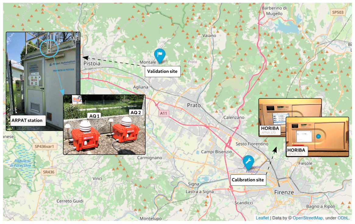
Figure 1 Map highlighting the calibration and validation locations for AQ1 and AQ2 LC air quality monitoring stations in Tuscany, Italy. At the calibration site (Florence), the HORIBA instruments used for calibrating the LC stations are shown, while at the validation site (Montale), the LC stations are pictured as installed on the roof of the reference ARPAT station (air quality station EoI code IT1553A).

2.3 Sensor calibration

As detailed in Table S1 in the Supplement, the pre-deployment calibration of the AQ1 and AQ2 stations against HORIBA analysers was performed at CNR–IBE headquarters in Florence, Italy (43^∘47^′52^′′ N, 11^∘11^′ E; Fig. 1). The AQ stations were mounted on a dedicated outdoor rack, while the HORIBA instruments were placed indoors in a laboratory setting. For outdoor air pollution sampling, approximately 2 m long sampling probes were employed to collect outside air and channel it directly to each of the reference instruments. HORIBA returned measurements at 3 min resolution collected across a 73 d period (19 July 2017–30 September 2017). To ensure data validity, measurements associated with RH >99 %, following Wang et al. (2010), or classified as outliers by an interquartile range (IQR) method (Dekking et al., 2005) were removed from the dataset, eventually resulting in 58 949 valid records for NO₂ and 59 261 valid records for O₃ concentrations. The workflow of the pre-deployment calibration process is shown in Fig. 2.

Prior to implementing the calibration techniques, an exploratory data analysis (EDA) was conducted using the correlation matrix to identify important insights. The study further explored the potential generalizable aspect of the relationship between O₃ MOSs and temperature, as highlighted in Spinelle et al. (2016), leveraging observations from the correlation matrix. The core of the calibration framework consisted of a set of supervised learning algorithms, previously evaluated in the literature, that fall into the following two categories: univariate and multiple models. The former are based on a single predictor (pollutant raw data), while the latter include additional predictors. Both categories included linear and non-linear algorithms. During the training phase, the datasets containing both LC and reference measurements were divided into a training subset consisting of 67 % of the data and a testing subset consisting of the remaining 33 %.

The suite of algorithms for univariate calibration linear methods included linear regression (Mijling et al., 2018; Maag et al., 2016) and robust regressions (Cavaliere et al., 2018), while the non-linear approaches comprised support vector machine (Bigi et al., 2018; Gu et al., 2018), random forest (Han et al., 2021; Zimmerman et al., 2018), and gradient boosting (Lin et al., 2018; Johnson et al., 2018). Multiple models, which considered temperature, humidity, and cross-sensitivity parameters for prediction, consisted of both parametric models and non-parametric models (Gäbel et al., 2022; Sayahi et al., 2020; Spinelle et al., 2017).

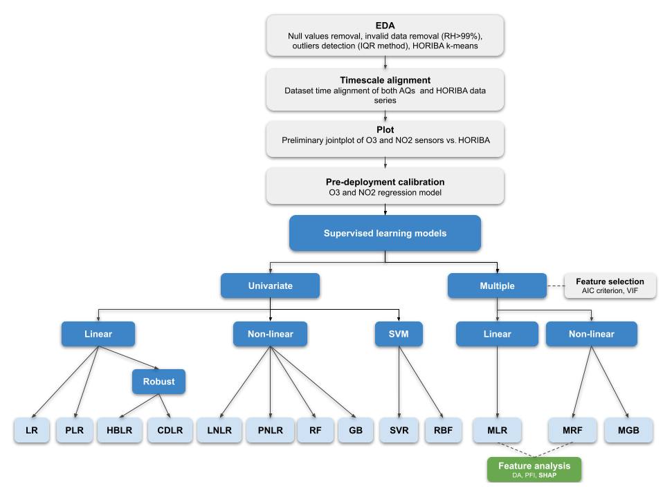
Figure 2 Workflow of the pre-deployment calibration process performed in the work. The model abbreviations are also listed in the Appendix.

2.3.1 Univariate models

The suite of univariate algorithms included a total of 10 models that fall into the following three main categories: (i) simple linear regression (SLR), (ii) non-linear regression (SNLR), and (iii) support vector machine (SVM). Five regression models are included in SLR, namely linear regression (LR); polynomial regression of the second (PLR2) and third (PLR3) degree; Huber regression (HBLR), which is a robust regression technique to outliers that uses a different loss function rather than the traditional least squares; and Cook's distance regression (CDLR; Cook, 1977), which summarizes how much all values in the regression model change when the ith observation is removed. The non-linear regression (SNLR) included parametric and non-parametric models. The former included power non-linear regression (PNLR) and logarithm regression (LNLR), which consider the estimation of coefficients through the Levenberg–Marquardt algorithm. The latter included random forest (RF) and gradient boosting (GB). RF conducts the optimal splitting of data samples into smaller sample sets, which then are fitted, respectively, along the tree paths, while GB built an additive model based on gradient boosting decision trees and in each stage in which a regression tree was fit. In the present calibration, the RF model used the mean square error as a fitting function in order to evaluate each decision split. Finally, SVM included a support vector regression using linear kernel (SVR) and radial basis function (RBF). In SVM, the kernel allows us to identify a hyperplane with maximum margin such that the maximum number of data points is within that margin. For each non-parametric model, the grid search method was used to optimize the default hyper parameter values (Pedregosa et al., 2011; Smets et al., 2007).

2.3.2 Multiple models

Multiple models included both linear (MLR) and non-linear models, with the latter consisting of multiple random forest (MRF) and multiple gradient boosting (MGB). While implementing an MLR model, a linear stepwise multi-regression analysis was carried out by automatically generating all possible models, starting from a list of explanatory variables. In the case of NO₂ and O₃ sensors, the latter included internal temperature (intT), external temperature (extT), and relative humidity (RH). In order to solely include statistically significant variables, thus excluding possible collinearity between them, the variance inflation factors (VIFs) were examined for each generated model. To refine the choice between internal and external temperature, a multiple linear model was used that alternatively incorporated both temperatures, followed by a cross-validation. Once a subset of significant explanatory variables was identified during the multiple linear regression (MLR) implementation, the multiple random forest (MRF) and multiple gradient boosting (MGB) models were also applied. MGB was selected, as GB is the univariate model that improves the results obtained by the supervised machine learning model, while MRF was selected as being a model that is widely used in the literature (e.g. Bisignano et al., 2022; Bigi et al., 2018; Zimmerman et al., 2018). To compare the performance between models, specified metrics were evaluated, such as the adjusted R² (AdjR²; Draper and Smith, 1998). In Table S2, a concise summary of the initialization hyperparameters applied to the models is provided.

2.3.3 Multiple-model interpretation

To gain a better understanding of the impact due to different predictors and an insightful interpretation of the multiple-model results, several analysis techniques have been applied, such as permutation feature importance (PFI; Breiman, 2001), dominance analysis (DA; Azen and Budescu, 2003), and the SHapley Additive exPlanation (SHAP; Lundberg and Lee, 2017) analysis.

PFI is a model inspection technique that measures the global variable importance by observing the effect of randomly shuffling each explanatory variable. DA is a common procedure for identifying the relative importance of predictors in a linear model. In this work, the following five different DA statistics were evaluated: (i) interactional dominance (IntD); (ii) individual dominance (ID); (iii) average partial dominance (APD); (iv) total dominance (TD); and (v) percentage relative importance (PRI).

SHAP analysis is a model-agnostic approach based on the game theory that can be applied to any machine learning model as a post hoc interpretation technique. According to the SHAP analysis, each machine learning model's prediction, f(x), can be represented as the sum of its computed SHAP values, plus a fixed base value, as shown in Eq. (1):

$$\begin{array}{}\text{(1)}& f\left(x\right)={\mathrm{\Phi }}_{\mathrm{0}}+\sum _{i=\mathrm{1}}^p{\mathrm{\Phi }}_i,\end{array}$$

where Φ₀ is the base value of the model, which represents the average prediction across all inputs, and Φ_i is the SHAP value for feature i for the input x. Each Φ_i is computed as in Eq. (2):

$$\begin{array}{}\text{(2)}& {\mathrm{\Phi }}_i=\sum _{S\subseteq \mathrm{1},\mathrm{2},\mathrm{\dots },p\setminus i}{\displaystyle \frac{(p-|S|-\mathrm{1})\mathrm{!}\cdot \left|S\right|\mathrm{!}}{p\mathrm{!}}}\cdot \left[f\right(x_{S\cup i})-f(x_S\left)\right],\end{array}$$

where p is the total number of features, S is a subset of all features except for feature i, $\left|S\right|$ is the number of features in subset S, f(x_S) is the model's prediction for input x with features in subset S, and f(x_S∪i) is the model's prediction for input x with features in subset S and feature i included.

SHAP values are calculated for each feature and value present in the dataset, and they approximate the contribution towards the output given by that data point. To compute SHAP values for different types of machine learning models, various SHAP implementations are available. In this study, the shap.LinearExplainer function was used for MLR predictors, while the FastTreeSHAP explainer (Yang, 2021) was used for other models. Compared to the widely used TreeSHAP algorithm, FastTreeSHAP provides faster computation of feature importance values for tree-based models.

2.4 Field validation

To test pre-deployment calibration models, the AQ stations were subject to a field validation based on hourly measurements collected during 429 consecutive days (19 June 2018–22 August 2019) by a reference air quality station operated by the Regional Agency of Tuscany for the Environmental Protection (ARPAT). High-resolution NO₂ and O₃ concentrations measured by the AQ stations over the same period were averaged hourly in order to be aligned to the reference data. Overall, datasets of valid hourly records, ranging 7383–9340 for NO₂ and 7344–9303 for O₃ concentrations, were used (Table S1). The reference air quality station (EoI code IT1553A) was located at Montale, a small town in Tuscany located between the cities of Prato and Pistoia (43^∘54^′57^′′ N, 11^∘00^′26^′′ E) and classified as a suburban background station (Fig. 1). The ARPAT reference station and the HORIBA APNA-370 analyser used the same method for measuring NO₂, while a different method (ultraviolet photometry) was used by ARPAT to measure O₃.

2.5 Statistics and libraries

The performances of each AQ station during both pre-deployment calibration and field validation were computed using various statistical measures, including the Pearson correlation coefficient (r); coefficient of determination (R²); AdjR²; root mean squared error (RMSE); normalized RMSE (nRMSE), which takes into account the range of values by dividing the RMSE by the difference between the maximum and minimum values; mean absolute error (MAE); and mean bias error (MBE). The variance impact factor (VIF) and Akaike information criterion (AIC) were also applied to discriminate between MLR models. All calculations related to calibration procedure and the analysis of the performance of the calibrated units are implemented using Python scikit-learn library (Pedregosa et al., 2011) and Python statsmodels module (Seabold and Perktold, 2010). Finally, a feature evaluation of MLR and MRF models was performed using the Python Dominance-Analysis library (Shekhar et al., 2019), SHAP library (Lundberg and Lee, 2022), FastTreeSHAP library (Yang, 2022), and ELI5 Permutation Importance library (TeamHG-Memex, 2022).

3 Results

3.1 Exploratory data analysis

After applying the humidity threshold and IQR procedure, 2 % and 12 % of the records were withdrawn from the initial datasets of the AQ1 and AQ2 stations, respectively. The comparison between the resulting O₃ and NO₂ data and the HORIBA reference concentrations is shown in Fig. 3. Based on the analysis of Pearson's correlation (Fig. S3), three patterns for both AQ stations emerged as conforming to the existing literature. HORIBA NO₂ and O₃ had a negative Pearson's r ($r_{\mathrm{AQ}\mathrm{1}}=-\mathrm{0.77}$; $r_{\mathrm{AQ}\mathrm{2}}=-\mathrm{0.75}$), which is compatible with the chemical coupling of O₃ and NO_x = NO + NO₂ (Han et al., 2011). AQ intT had a high positive correlation with HORIBA O₃ (r_AQ1=0.79; r_AQ2=0.80), which is compatible with the fact that high temperatures can increase the rate of O₃ formation through photochemical reactions (Han et al., 2011). AQ RH had a high negative correlation with HORIBA O₃ ($r_{\mathrm{AQ}\mathrm{1}}=-\mathrm{0.75}$; $r_{\mathrm{AQ}\mathrm{2}}=-\mathrm{0.74}$), which is compatible with the fact that high relative humidity is generally associated with lower O₃ levels (Camalier et al., 2007). Moreover, as a result of the convective heat transfer equation, a strong positive correlation was observed between intT and extT for each AQ ($r_{\mathrm{AQ}\mathrm{1},\mathrm{AQ}\mathrm{2}}=\mathrm{1}$). On average, the temperature difference between intT and extT remains relatively constant at around 8 ^∘C. A visual representation of the difference between the two temperatures, plotted against their mean, can be found in the Bland–Altman plots in Fig. S4. No significant correlation was observed between NO₂ raw and either temperature or RH. Moderate positive associations were instead found between O₃ raw and both intT (r_AQ1=0.55; r_AQ2=0.55) and extT (r_AQ1=0.52; r_AQ2=0.53).

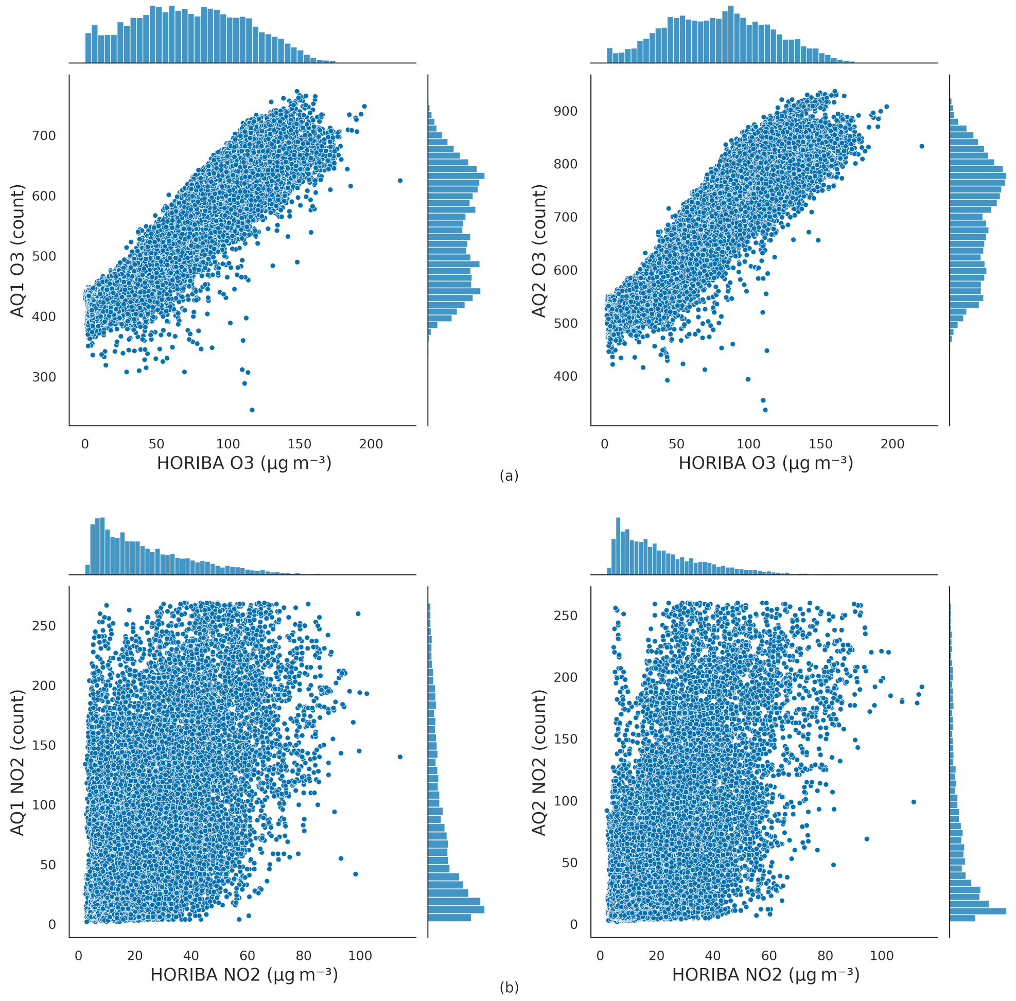
Figure 3 Scatterplots of 3 min sampled AQ1 and AQ2 signals vs. HORIBA reference concentrations observed during the pre-deployment calibration for O₃ (a) and NO₂ (b).

3.2 Univariate models

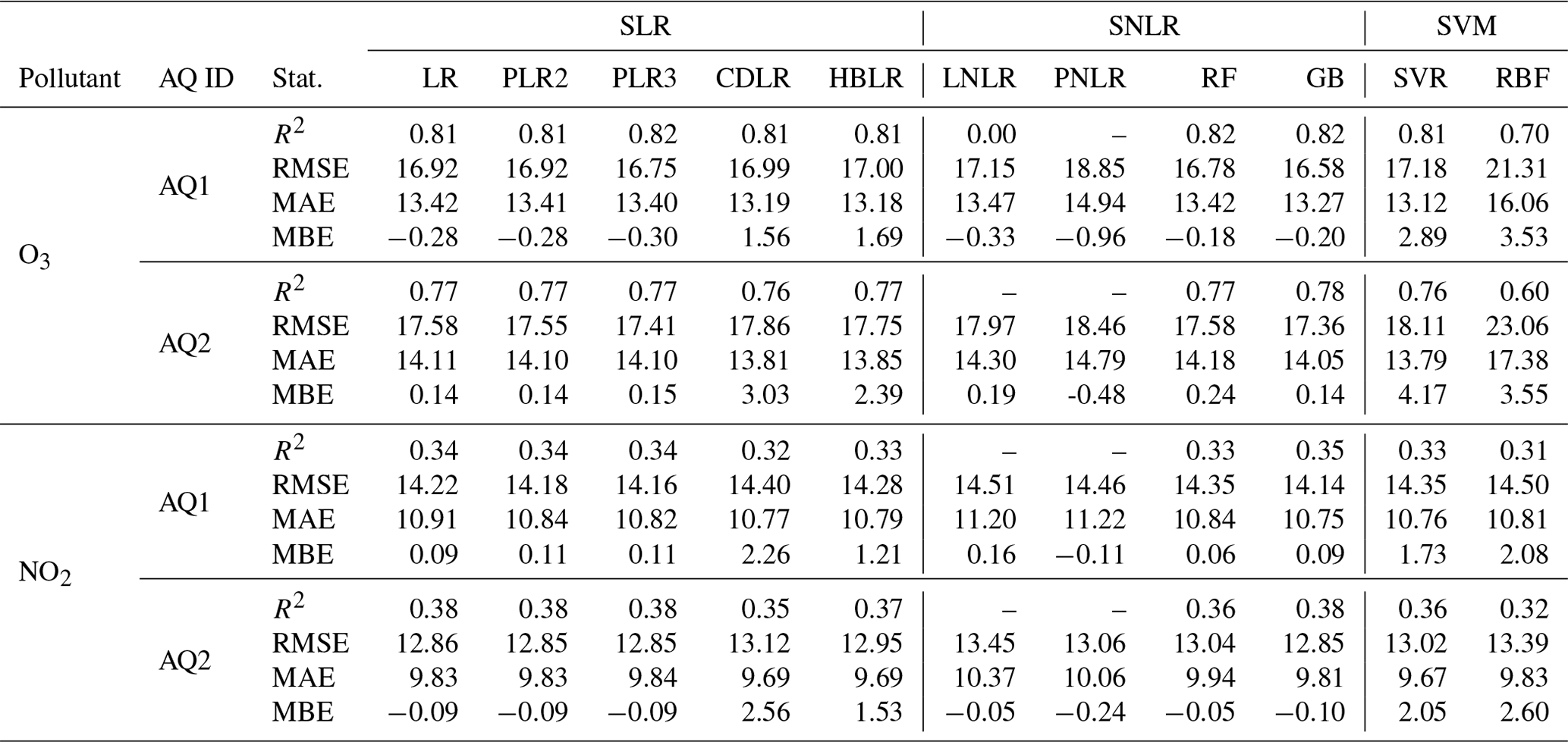
The results of the supervised linear (SLR), supervised non-linear (SNLR), and support vector machine (SVM) models applied for both AQ stations and pollutants are reported in Table 1. For both AQ stations, the best performances were found using the GB model, with O₃ concentrations generally fitting better than NO₂ concentrations.

Table 1 Statistics of the univariate regression models applied to the AQ1 and AQ2 stations. Note that for non-linear models (LNLR and PNLR), R² is not a useful metric, while it is useful for linear models that use polynomials to model the curvature in the data (Spiess and Neumeyer, 2010).

3.3 Multiple regression

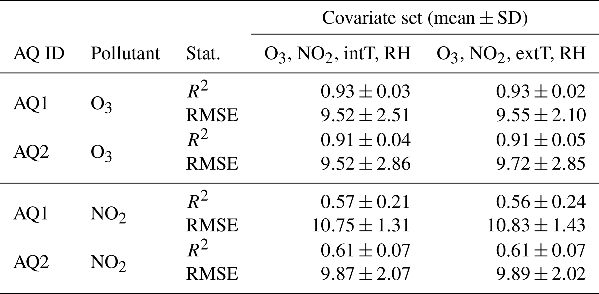
EDA suggested that the inclusion in multiple regression models of both intT and extT may result in unstable results due to their strong collinearity ($r_{\mathrm{AQ}\mathrm{1},\mathrm{AQ}\mathrm{2}}=\mathrm{1}$). This was confirmed by the variance inflation factor (VIF) for the MLR model, which was higher than 5 when both variables were used (Table S5). To ensure consistent selection of the optimal temperature variable in the model, a cross-validation procedure was conducted on the calibration dataset for the MLR model, alternately including intT and extT in the covariate set. The results of the five-split cross-validation (Table 2) showed no significant differences when using intT or extT, while the use of intT provided a slightly higher mean accuracy and a lower mean RMSE.

Table 2 R² and RMSE (µg m⁻³) values by covariate set, including intT or extT variables of the cross-validation procedure applied to the MLR model.

Following the previous result, the final subset of predictors used for all models consisted of intT, RH, and raw signal from both sensors (Tables S6 and S7). Accordingly, for both stations, Eqs. (3) and (4) were the best model formulas for O₃ and NO₂ sensors, respectively:

$$\begin{array}{}\text{(3)}& {\displaystyle }\begin{array}{rl}{\mathrm{O}}_{\mathrm{3}}& ={\mathit{\beta }}_{\mathrm{0}}+{\mathit{\beta }}_{\mathrm{1}}\cdot {\mathrm{NO}}_{\mathrm{2}}\mathrm{raw}+{\mathit{\beta }}_{\mathrm{2}}\cdot {\mathrm{O}}_{\mathrm{3}}\mathrm{raw}\\ & +{\mathit{\beta }}_{\mathrm{3}}\cdot \text{RH}+{\mathit{\beta }}_{\mathrm{4}}\cdot \text{intT}\end{array}\text{(4)}& {\displaystyle }\begin{array}{rl}{\mathrm{NO}}_{\mathrm{2}}& ={\mathit{\beta }}_{\mathrm{0}}+{\mathit{\beta }}_{\mathrm{1}}\cdot {\mathrm{NO}}_{\mathrm{2}}\mathrm{raw}+{\mathit{\beta }}_{\mathrm{2}}\cdot {\mathrm{O}}_{\mathrm{3}}\mathrm{raw}\\ & +{\mathit{\beta }}_{\mathrm{3}}\cdot \text{RH}+{\mathit{\beta }}_{\mathrm{4}}\cdot \text{intT}.\end{array}\end{array}$$

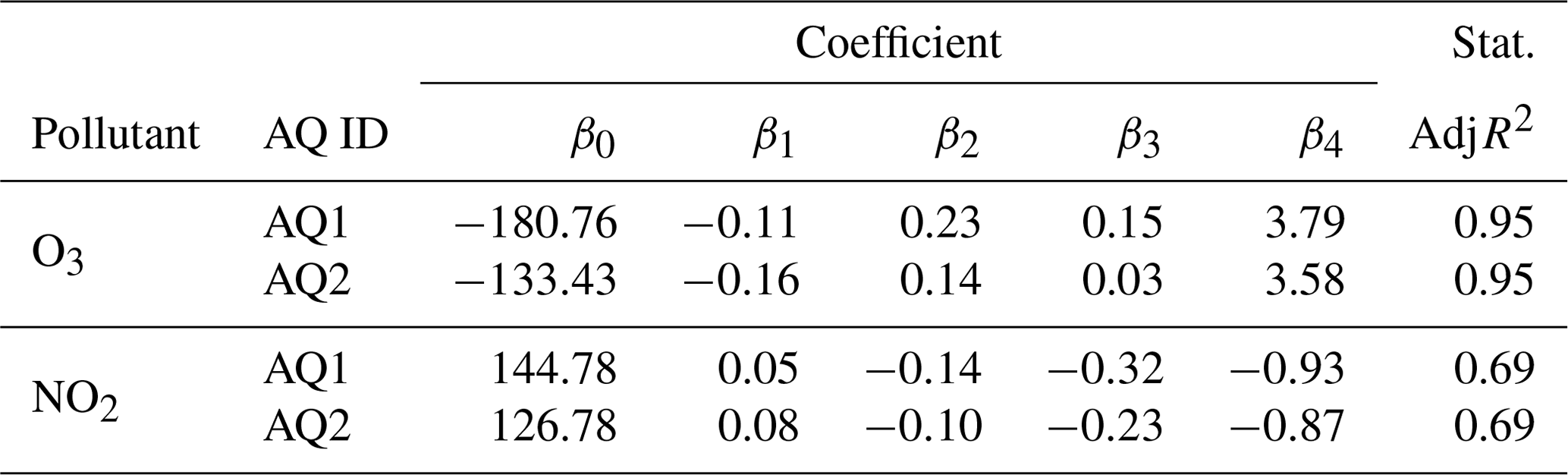
The calibration coefficients achieved for the MLR model are reported in Table 3, while the scores of the MLR, MGB, and MRF model application are reported in Table 4.

Table 3 Statistics of the MLR model applied to the AQ1 and AQ2 stations. β₀ values are the intercepts, and β_i values are the calibration coefficients.

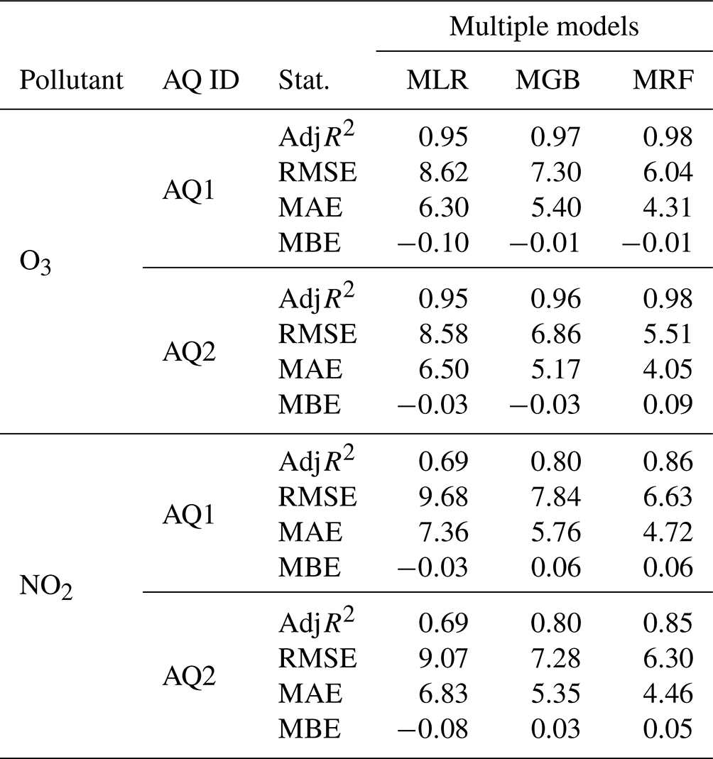
Overall, O₃ concentrations were better fitted than NO₂ concentrations, while MRF proved to be the finest model, generally outperforming the MGB and particularly the MLR model.

Table 4 Statistics of the multiple regression models applied to the AQ1 and AQ2 stations.

3.4 Multiple-model interpretation

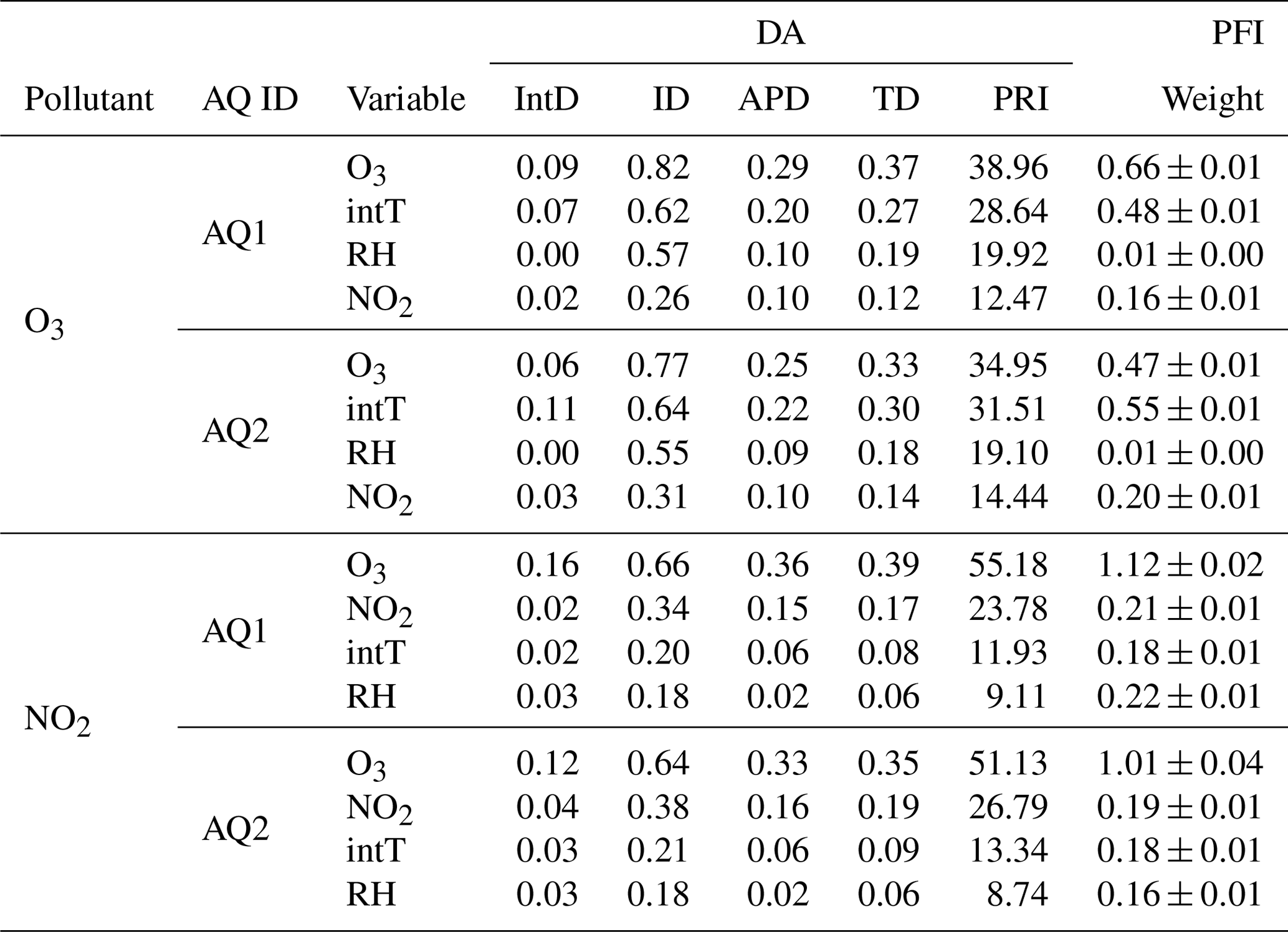
In terms of traditional statistical inference techniques such as DA and PFI during MLR and MRF O₃ calibration, the results confirmed first O₃ raw and second intT as being the most significant predictors (Table 5), which were consistent with those reported by Masson et al. (2015). Overall, the DA analysis showed that O₃ raw and intT were the most important features for both stations and pollutants. In particular, for O₃ concentrations, O₃ raw data resulted in the highest PRI value, explaining 38.96 % and 34.95 % of the R² of the MLR model for AQ1 and AQ2, respectively, followed by intT (28.64 % and 31.51 %, respectively). Also for NO₂ concentrations, O₃ raw data had the highest PRI value, explaining 55.18 %–51.13 % of the R² of the MLR model, followed by NO₂ raw data (23.78 %–26.79 %). In the O₃ MRF regression, O₃ raw was the most important feature for AQ1, while it was intT for AQ2. Conversely, in the NO₂ MRF regression, O₃ raw was the most important feature for both AQ stations, followed by RH for AQ1 and by NO₂ for AQ2. Notably, for both MLR and MRF models, O₃ raw proved to be a more important feature in NO₂ calibration than in O₃ calibration.

Table 5 DA statistics and PFI weights achieved for MLR and MRF models and applied to the AQ1 and AQ2 stations.

The challenge with traditional feature selection methods like DA and PFI is that they may produce misleading results when features are highly correlated or the data are noisy. These methods in fact do not consider interactions or correlations between predictors, and DA is only applicable to linear models. To overcome these limitations, the study utilized SHAP analysis. The SHAP analysis was performed in order to gain insight into both the global and local contribution of each feature at both individual instance level and across the population, resulting in the SHAP bee swarm plots for MLR and MRF, as shown in Figs. 4 and 5, respectively. The bee swarm plot ranks the input features from the highest to the lowest mean absolute SHAP values for the entire dataset. For each variable, every instance of the dataset appears as its own point. The points are distributed horizontally along the x axis according to their SHAP value. In places where there is a high density of SHAP values, the points are stacked vertically. The colour bar corresponds to the raw values of each feature for each instance, providing a visual representation of the feature's contribution to the outcome prediction.

Figure 4 Bee swarm plot showing the SHAP values calculated for each feature and instance using the linear explainer the MLR model for O₃ (a) and NO₂ (b).

Figure 5 Bee swarm plot showing the SHAP values calculated for each feature and instance using the FastTreeSHAP of the MRF model for O₃ (a) and NO₂ (b).

As for the MLR model for both AQ stations, high levels of both O₃ raw and intT data had a strong and positive impact on O₃ output, as indicated by high and positive SHAP values (Fig. 4a), while high levels of NO₂ raw data had a strong and positive impact on the NO₂ output (Fig. 4b). Herein, however, high levels of O₃ raw and intT data had a greater impact on decreasing the predicted values of NO₂ than the raw data of NO₂.

Also, for the MRF model, O₃ raw data had a high influence on O₃-predicted values (Fig. 5a) because higher values of O₃ raw data increased the O₃ prediction, while lower values had a negative effect. This also applies to the NO₂ output values (Fig. 5b), as higher values of O₃ raw data decreased the NO₂ prediction and lower values had a positive effect. Herein, however, high or low levels of NO₂ raw had no significant influence on the prediction. The mean absolute SHAP values for all features of both MLR and MRF models are reported in Fig. S8.

In order to provide a local interpretability, a heatmap for the SHAP values of the NO₂ MLR model was also elaborated (Fig. 6). The heatmap showed that lower model predictions f(x), computed using Eq. (1), were linked to a dark colour for O₃ and a light colour for NO₂ for both AQ stations. This suggested that O₃ raw data had a more significant impact, mostly on the lower NO₂ concentrations than the NO₂ raw data had, while the impact of the NO₂ raw data became significant at higher concentrations.

Figure 6 Heatmap of SHAP values of the NO₂ MLR model for AQ1 (a) and AQ2 (b). The heatmap displays the contribution of each feature to the model's predictions, with positive contributions represented by dark-coloured cells and negative contributions by light-coloured cells. The colour intensity denotes the magnitude of the contribution. The output of the model, f(x), is shown above the heatmap matrix, which is centred around the explanation's base value (ϕ₀), and the global importance of each model input is shown in the bar plot on the right-hand side of the plot. Observations have been ordered by the sum of the SHAP values over all features.

3.5 Field validation

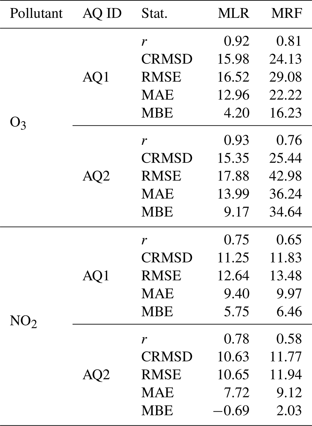
The scores of field validation involving the MLR- and MRF-calibrated models are summarized in Table 6. Model accuracy in predicting the O₃ concentrations is confirmed to be higher than in predicting the NO₂ concentrations. In terms of Pearson's r values, the MLR model outperforms the MRF model, exhibiting r values (0.92–0.93 for O₃ and 0.75–0.78 for NO₂) higher than MRF (0.81–0.76 for O₃ and 0.76–0.65 for NO₂), while the opposite applies in terms of the standard deviation, as MRF returns lower values than MLR. Notably, a significant difference by AQ station may be observed in MRF scores, while it is not the case for MLR.

Taylor diagrams of the pre-deployment MLR- and MRF-calibrated models assessed against the ARPAT reference station for O₃ (Fig. S10a) and NO₂ (Fig. S10b) concentrations may be found in Fig. S10, while weekly concentrations predicted by the models against the reference station are given in Fig. 7.

Figure 7 Trend analysis of 7 d average O₃ and NO₂ concentrations measured at the validation site by the calibrated AQ1 and AQ2 stations compared to the ARPAT reference station (17 June–22 August 2019).

Table 6 Statistics of the MLR- and MRF-calibrated models assessed during the field validation procedure. CRMSD is the centred root mean squared difference.

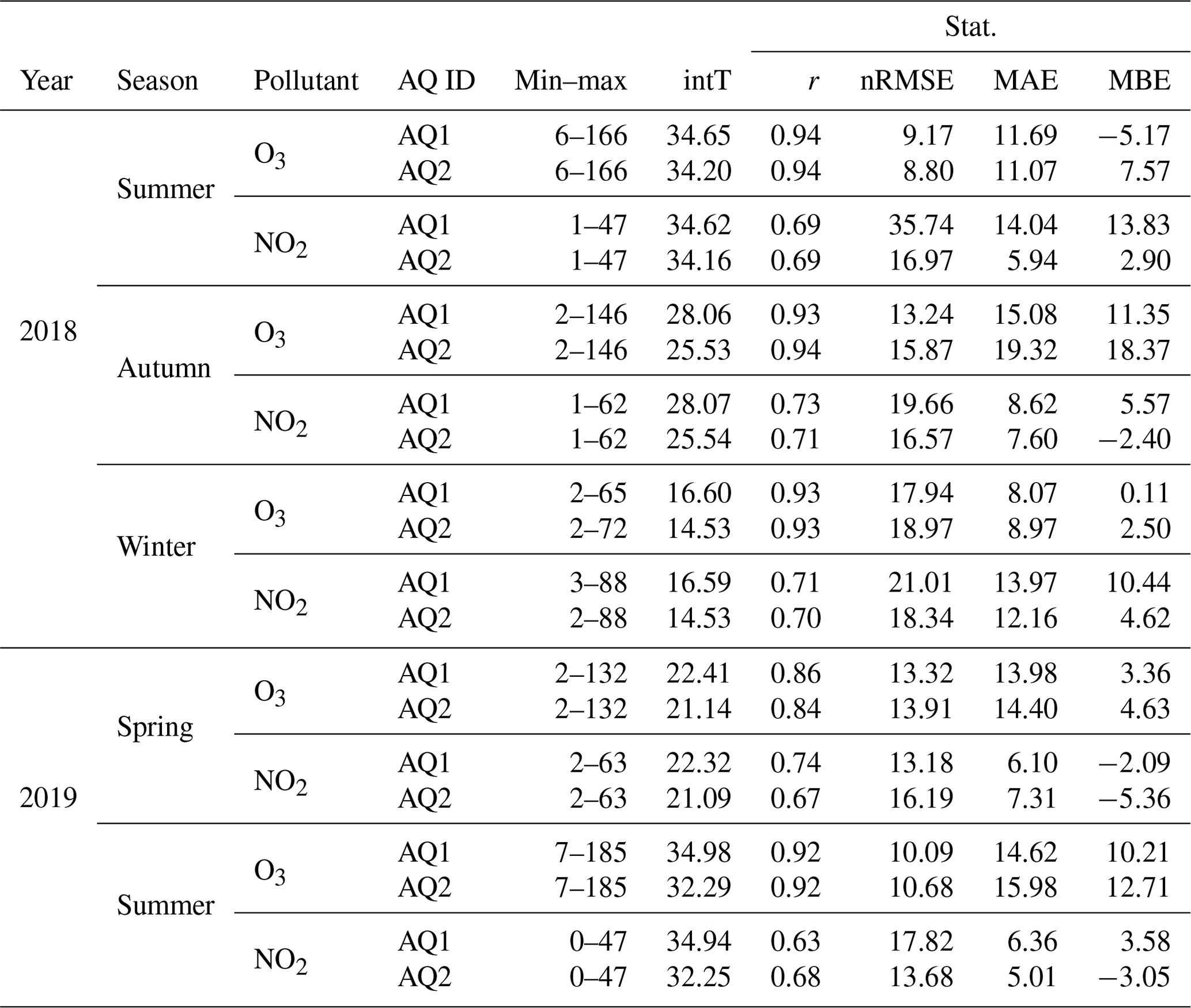
A seasonal analysis was also performed for MLR field validation (Table 7). O₃ concentrations were well predicted across all seasons; for both stations, the lowest nRMSE values were registered in the summers of 2018 and 2019 and the highest in winter from 2018–2019. Notably, all statistical scores during the summer in 2019 proved to be worse compared to the summer in 2018, suggesting a likely drift in sensor accuracy after 1 year of deployment. As for NO₂, the highest (and thus more meaningful) concentrations were measured in winter from 2018–2019. The NO₂ scores during this period, however, are confirmed to be worse than those affecting O₃ during the period of highest O₃ concentrations (i.e. summers of 2018 and 2019). Furthermore, the scores of seasonal analysis addressed for MRF field validation may be found in Table S12.

Table 7 Seasonal analysis of MLR validation. Minimum and maximum values (µg m⁻³) represent the minimum and maximum concentrations measured by the reference station, while intT (^∘C) is the average internal temperature measured by the AQ stations.

4 Discussion

Current outcomes achieved for the MOS O₃ and NO₂ pre-deployment calibration were generally consistent with those found in the literature. MOS NO₂ calibration exhibited low accuracy in linear univariate models, as demonstrated by Nowack et al. (2021), and the MiCS-2710 NO₂ sensor achieves a poor R² (0.21) compared to the O3_3E1F EC sensor value (0.845), as reported by Spinelle et al. (2015). In contrast, the O₃ sensor calibration returns high R² values, suggesting limited potential for improvement using more complex univariate techniques like SVR, RF, or GB, as noted in Sales-Lérida et al. (2021). For the NO₂ calibration, incorporating multiple covariates like temperature, humidity, and gaseous interference compounds was instead essential for better performance, as emphasized in studies cited in Karagulian et al. (2019).

This study confirmed that both linear and non-linear multiple models resulted in a slight improvement in the O₃ calibration and a significant one in the NO₂ prediction when compared to univariate models (Table 4). In particular, the MLR model improved the accuracy of the simple LR by more than 14 %–18 % for O₃ and 31 %–35 % for NO₂. Notably, both MOSs performed well when using the same model form, but due to intersensor variability, each sensor necessitated a distinct set of coefficients to achieve optimal performance. Moreover, taking into account the observed multicollinearity issue between temperatures and the slightly higher mean accuracy, as well as the lower mean RMSE observed when using the internal one (Table 2), the study drew upon insights from existing literature to identify the most suitable set of covariates (e.g. Miech et al., 2021; Schmitz et al., 2021). As a result, the inclusion of internal temperature as a significant factor was given priority, as it offers a more accurate representation of the operating conditions of the MOSs within the system. This approach was also adopted to tackle potential challenges in the board's analogue-to-digital converter circuit.

However, among the multiple models, MRF proved to be the most effective in the pre-deployment calibration (e.g. Bisignano et al., 2022; Johnson et al., 2018). The SHAP methodology proved to be particularly insightful in gaining a comprehensive understanding of the behaviour of both MLR and MRF models in the pre-deployment calibration dataset. It enabled the identification of the relationships between input features (O₃, NO₂, internal temperature, and relative humidity) and the predicted outcomes. Additionally, the use of SHAP allowed for the diagnosis of potential issues, such as the non-parametric models' ability to extrapolate and predict pollution levels beyond the scope of the training calibration dataset (e.g. Nowack et al., 2021; Malings et al., 2019). These issues were confirmed through the validation process against ARPAT official reference.

As evident from Table 7, the MLR calibration model outperformed the MRF approach, thus showcasing a better transferability across diverse spatial and temporal settings. Besides, even though the pre-deployment dataset mainly represented a summer period, the physical patterns identified in the MLR model remained valid across seasons. Additionally, the SHAP heatmap (Fig. 6) provided insightful evidence of the O₃ sensor's ability to handle the lower reading limit of the NO₂ sensor for both AQ stations. This observation is important, especially in conditions with low-NO₂ concentrations, where the NO₂ sensor's accuracy in providing readings might be compromised.

On the contrary, MRF did not align perfectly with the expected underlying physical model. Instead, it appeared to be “true to the data”, due to its ability to memorize specific patterns from the pre-deployment dataset, based on what emerged by the SHAP analysis (Fig. 6b). However, this characteristic posed challenges when trying to apply the model to unseen data, leading to unsatisfactory performance in the field. This lack of generalization capability hindered the MRF model's effectiveness when faced with differing concentration regimes.

The seasonal analyses presented in Table 7 provided an overview of these seasonal changes in the stability and biases of the AQ1 and AQ2 O₃ and NO₂ sensors for the application of the MLR calibration model after deployment. The O₃ pre-deployment calibration showed good performance in all seasons, and for both stations, the lowest nRMSE value was registered in summer 2018 and in summer 2019, and the highest value of nRMSE was recorded in winter 2018–2019. The decline in performance during the winter period was minimal, despite the fact that the pre-deployment calibration was mainly performed in the summer. Furthermore, a comparison of the summer period of 2018 and 2019 showed a decrease of 2 % in nRMSE for both AQ stations and pollutants (O₃ and NO₂). The decrease in nRMSE for O₃ was accompanied by an increase in the magnitude of MAE and MBE, pointing towards a possible linear drift in the O₃ sensor readings after a year of use. Conversely, for pre-deployment calibration of NO₂, a decrease in MBE was observed. The decrease in MBE for NO₂ and the prominent role of O₃ raw readings and its negative impact on prediction, as identified through feature importance analysis of the pre-deployment MLR model, further reinforced the idea of a linear drift in O₃ sensor readings. Similarly, the pattern of the lowest and highest nRMSE values for O₃ validation also remained consistent for the MRF model, with the values being the lowest in the summer of 2018 and 2019 and the highest in the winter of 2018–2019 (Table S12). Notably, AQ1 outperforms AQ2 in both models; however, as mentioned earlier, the differences in nRMSE values between the MLR and MRF models were quite significant.

5 Conclusions and perspective

In this study, the pre-deployment calibration and field validation of two low-cost (LC) stations named AirQino, developed by CNR–IBE in Florence (Italy), were addressed. The stations were equipped with O₃ and NO₂ MOSs and meteorological sensors. Pre-deployment calibration was performed after developing and implementing a comprehensive calibration framework, consisting of several elements, including parametric, non-parametric univariate, and multiple algorithms, that allowed us to identify the optimal calibration pathway. Ultimately, this resulted in robust LC performances outside the training conditions and the ability for easy adjustments to cope with changes in sensor performance over time. While selecting the most suitable LC calibration models, necessarily going beyond mere accuracy, this study primarily recommends (i) including multiple covariates, such as internal (rather than external) temperature, relative humidity, and gaseous interference compounds, into the multiple regression models and (ii) analysing the importance of the features used in the multiple models to disclose their role when the calibrated LC stations are operated under field conditions rather than in a controlled environment.

As a novelty applied to LC MOS calibration, the SHapley Additive exPlanations (SHAP) method was used to provide further insight into the role played by individual model predictors and their global and local impact on the overall LC sensor performances. This method was also used to hypothesize the capability of the model to accurately describe conditions beyond the pre-deployment calibration period.

This study confirmed that machine learning models, such as MRF, can effectively calibrate LC sensors and mitigate the impact of environmental conditions and pollutant cross-sensitivity. However, while the MRF model demonstrated higher accuracy than MLR during pre-deployment calibration, it faced challenges in accurately representing physical models and struggled to generalize on the field validation dataset. Furthermore, as well as being less computationally demanding and generally more suitable for non-experts, parametric models such as MLR have a defined equation that also includes a few parameters, which allows – when needed – easy adjustments for possible changes over time. Thus, drift correction or periodic automatable recalibration operations can be readily scheduled, making parametric models advantageous. This aspect is particularly relevant for NO₂ and O₃ MOSs, as demonstrated in this study. Both sensors performed well with the same linear model form, requiring unique parameter values due to intersensor variability.

A limitation of the present work is that the LC stations have been calibrated during a period that is not particularly long (73 d) and a typically summer period, thus when pollution levels are generally meaningful for O₃, but they are not meaningful for NO₂ concentrations. Indeed, conducting a pre-deployment calibration during a winter period, when NO₂ concentrations are typically higher, would be a valuable addition to the study. This step would provide a more comprehensive understanding of the AQ station validation performance under varying pollution conditions and help address the limitation of the current calibration period biased towards summer data. Moreover, conducting a similar validation outside of Italy, in regions with differing pollution and meteorological conditions, would be of great interest. For this purpose, in the ongoing activity, the AirQino LC stations are planned to be deployed outside Italy, such as in Nice and Aix-en-Provence (France), Barcelona (Spain), Budapest (Hungary), Tirana (Albania), and Niamey (Niger).

Furthermore, in the future, a new sensor for monitoring NO could hopefully be integrated into the LC stations and validated. As such, the combined monitoring of NO, NO₂, and O₃ concentrations and their daily and seasonal variability would allow a comprehensive pattern of the oxidant capacity of atmosphere, which is particularly effective in southern Mediterranean countries such as Italy (Pancholi et al., 2018). In addition, once the AQ VOC sensor is validated, it will enable the monitoring of all O₃ precursors (VOC and NO_x). This comprehensive monitoring, combined with the application of SHapley Additive exPlanations (SHAP) method, will lead to a full characterization of photochemical pollution in various areas of interest, including urban, sub-urban, or rural regions. Moreover, the portability of LC sensors makes them ideal devices for filling knowledge gaps in regions that are difficult to access, such as the open sea. When mounted on buoys or ships, for example, LC sensors could collect the high-O₃ levels that typically occur over these areas in summer due to high solar activity and rather low mixing height combined with a lack of O₃-consuming NO emissions.

Appendix A: Nomenclature

APD	Average partial dominance	LC	Low cost	RBF	Radial basis function
AQ	AirQino	LNLR	Logarithm regression	RF	Random forest
CDLR	Cook's distance regression	LR	Linear regression	RH	Relative humidity
DA	Dominance analysis	MGB	Multiple gradient boosting	SHAP	SHapley Additive exPlanations
EC	Electrochemical	MLR	Multiple linear regression	SLR	Supervised linear regression
EDA	Exploratory data analysis	MOS	Metal oxide sensors	SNLR	Supervised non-linear regression
extT	External temperature	MRF	Multiple random forest	SVM	Support vector machine
GB	Gradient boosting	PFI	Permutation feature importance	SVR	Support vector regression
HBLR	Huber regression	PLR2	Polynomial regression of second degree	TD	Total dominance
ID	Individual dominance	PLR3	Polynomial regression of third degree	VIF	Variance impact factor
IntD	Interactional dominance	PNLR	Power non-linear regression
intT	Internal temperature	PRI	Percentage relative importance