the Creative Commons Attribution 4.0 License.
the Creative Commons Attribution 4.0 License.
 | 27 Jan 2023
Field comparison of two novel open-path instruments that measure dry deposition and emission of ammonia using flux-gradient and eddy covariance methods
Daan Swart
Jun Zhang
Shelley van der Graaf
Susanna Rutledge-Jonker
Arjan Hensen
Stijn Berkhout
Pascal Wintjen
René van der Hoff
Marty Haaima
Arnoud Frumau
Pim van den Bulk
Ruben Schulte
Margreet van Zanten
Thomas van Goethem
Dry deposition of ammonia (NH3) is the largest contributor to the nitrogen deposition from the atmosphere to soil and vegetation in the Netherlands, causing eutrophication and loss of biodiversity; however, data sets of NH3 fluxes are sparse and in general have monthly resolution at best. An important reason for this is that measurement of the NH3 flux under dry conditions is notoriously difficult. There is no technique that can be considered as the gold standard for these measurements, which complicates the testing of new techniques. Here, we present the results of an intercomparison of two novel measurement set-ups aimed at measuring dry deposition of NH3 at half hourly resolution. Over a 5-week period, we operated two novel optical open-path techniques side by side at the Ruisdael station in Cabauw, the Netherlands: the RIVM-miniDOAS 2.2D using the aerodynamic gradient technique, and the commercial Healthy Photon HT8700E using the eddy covariance technique. These instruments are widely different in their measurement principle and approach to derive deposition values from measured concentrations; however, both techniques showed very similar results (r=0.87) and small differences in cumulative fluxes (∼ 10 %) as long as the upwind terrain was homogeneous and free of nearby obstacles. The observed fluxes varied from ∼ −80 to ∼ +140 ng NH3 m−2 s−1. Both the absolute flux values and the temporal patterns were highly similar, which substantiates that both instruments were able to measure NH3 fluxes at high temporal resolution. However, for wind directions with obstacles nearby, the correlations between the two techniques were weaker. The uptime of the miniDOAS system reached 100 % once operational, but regular intercalibration of the system was applied in this campaign (35 % of the 7-week uptime). Conversely, the HT8700E did not measure during and shortly after rain, and the coating of its mirrors tended to degrade (21 % data loss during the 5-week uptime). In addition, the NH3 concentrations measured by the HT8700E proved sensitive to air temperature, causing substantial differences (range: −15 to +6 µg m−3) between the two systems. To conclude, the miniDOAS system appears ready for long-term hands-off monitoring. The current HT8700E system, on the other hand, had a limited stand-alone operational time under the prevailing weather conditions. However, under relatively dry and low-dust conditions, the system can provide sound results, opening good prospects for future versions, also for monitoring applications. The new high temporal resolution data from these instruments can facilitate the study of processes behind NH3 dry deposition, allowing an improved understanding of these processes and better parameterisation in chemical transport models.
- Article
(6046 KB) - Full-text XML
-
Supplement
(5979 KB) - BibTeX
- EndNote


Human alteration of the global nitrogen cycle through agricultural, industrial, and combustion processes has led to unprecedented levels of reactive nitrogen (Nr) in the Earth system (Galloway et al., 2021; Fowler et al., 2013). Besides benefits, such as increased food production, losses of Nr have a range of detrimental effects on both the environment and human health (Sutton et al., 2011; Erisman et al., 2015). Gaseous NH3 can be emitted from and deposited onto the Earth's surface and the exchange is bidirectional. With respect to deposition, dry deposition of NH3 is an important component. In the Netherlands for example, it typically accounts for more than one third of the total Nr deposition (Hoogerbrugge et al., 2020). Accurate quantification of biosphere-atmosphere exchange of NH3 is therefore essential to increase our understanding of NH3 budgets on regional and global scales, to study relevant processes at high time resolution, monitor trends, measure the effectiveness of mitigation efforts, and improve and validate air quality and deposition models.
Despite the relevance of high-quality measurements of NH3 exchange, relatively few direct long-term continuous measurements have been reported. Dry deposition of NH3 can be highly variable in time and space and depends on a variety of site-specific parameters like canopy wetness, leaf area, and surface roughness (Flechard et al., 2011). Micrometeorological techniques provide the most direct estimates of dry deposition, but these measurements each present technical challenges and generally require substantial expense and labour.
The aerodynamic flux gradient method (AGM, also profile method) has delivered the majority of the NH3 dry deposition data worldwide. Most of these measurements were done using wet chemical instrumentation (e.g. Erisman and Wyers, 1993; Loubet et al., 2012), but nowadays also optical NH3 measurement systems are used (e.g. Kamp et al., 2020). In the AGM method, surface-atmosphere exchange fluxes are derived from measurements of vertical concentration differences ( combined with measurement of vertical turbulent transport (Loubet and Personne, 2016; Prueger and Kustas, 2005). Drawbacks of AGM (listed by Trebs et al., 2021; Loubet et al., 2013) include potentially biased gradients under nonstationary conditions if sequential sampling at multiple heights using one monitor is required (Kamp et al., 2020) or if using multiple monitors, there is a need for regular side by side comparisons to accurately determine and correct for any potential systematic difference (bias) between monitors (Wolff et al., 2010; Walker et al., 2013). Finally, a drawback of AGM is the need to rely on empirical stability corrections, which are based on relationships found for sensible heat, but assumed to be the same for trace compounds like NH3.
Open-path (OP) techniques avoid the delay effects, reduced temporal resolution and interference from aerosols that result from NH3 sticking to inlet lines, air filters and other surfaces in an instrument (Parrish and Fehsenfeld, 2000). The OP analysers have no sampling tubes and provide a way of measuring concentration in situ, without interfering with the airflow. A long path averaging OP gas analyser allows measurements of path-integrated NH3 concentrations at a high time resolution. Optical analysers now available include those based on Fourier transform infrared (FTIR) (Sintermann et al., 2011; Flesch et al., 2016), tuneable diode laser (TDL) (Bai et al., 2022) or differential optical absorption spectroscopy (DOAS) (Volten et al., 2012b; Sintermann et al., 2016). These instruments can be used to measure the difference in NH3 concentration between two vertically offset paths, either in slant configuration (e.g. Bai et al., 2021; Flesch et al., 2016) or in two parallel horizontal paths. In the Netherlands, several experiments have taken place using two DOAS systems to measure (Wichink Kruit et al., 2010; Volten et al., 2012a; Schulte et al., 2020). Over the last years, the more recently developed miniDOAS (Berkhout et al., 2017) has been adapted and improved to meet the high sensitivity required for flux gradient measurements of NH3 (Wolff et al., 2010; Foken, 2008).
Eddy covariance (EC) is the preferable technique for measuring the surface-atmosphere gas exchange of any compound because it provides the most direct measurement. However, EC requires fast (<0.1 s) and precise concentration measurements, which is particularly challenging for NH3. In recent years, several studies have reported measurements of the NH3 flux using closed-path (CP) analysers (Famulari et al., 2004; Moravek et al., 2019; Zöll et al., 2016). However, the reactivity and solubility of NH3 in water presents challenges there, because the use of inlet tubing leads to loss of fast variations in the signal.
So far, two folded-path OP instruments are available for eddy covariance measurements of NH3. Besides the benefit compared to the CP set-up of not needing an inlet tube, such systems generally have much lower power requirements and the less bulky installation may allow a more portable and adaptable set-up also at more remote sites.
The first OP EC NH3 analyser was the quantum cascade laser (QCL) based instrument developed by Princeton University, and improved from the original design presented in Miller et al. (2014) over various deployments (Sun et al., 2015; Pan et al., 2021). More recently, a similar instrument has become available from Healthy Photon Co. Ltd., Ningbo, China: model HT8700 (Wang et al., 2021). Limitations of OP EC flux measurements include interference from contamination by dust and rainfall, and the influence of exposure of the instrument to outdoor conditions. As this technique evaluates the net flux by measuring concentration levels in both upgoing and downgoing air that passes the sensing volume both in small, high-frequency (>5 Hz) eddies and in slow (>10 min) large turbulent eddies, the method needs corrections for differences in air density between upgoing and downgoing air. Similar to closed-path EC gas analysers, not all sizes and frequencies of eddies are measured completely and therefore (high and low frequency) spectral corrections are needed.
Both micrometeorological methods (AGM and EC) share additional limitations to those mentioned above, such as the need for a homogeneous upwind fetch to avoid local advection errors. They also require steady-state conditions and well-developed turbulence, with no change in vertical flux with height (Loubet et al., 2013; Mauder et al., 2021).
In this study, we measured bidirectional NH3 fluxes in a field campaign of 7 weeks from 24 August 2021 to 11 October 2021 over grassland at the Cabauw research site in the Netherlands, during which both deposition and emission events were encountered. During a period of 5 weeks (27 August to 1 October), we compared measurements of NH3 concentrations and fluxes from two OP instruments: the RIVM miniDOAS 2.2D using the AGM, and the commercial HT8700E from Healthy Photon Inc. using the EC technique. This was the first time either one of these systems was compared to another set-up. The primary aim of the campaign was to test if both novel instruments were indeed capable of measuring the dry exchange flux of NH3 at high temporal resolution. Here, we describe the uptime and performance of both set-ups and compare the results of both concentration and flux measurements of NH3. Moreover, potential sources of errors, challenges encountered and the current suitability and future potential of the different set-ups for long-term in situ measurements under field conditions are discussed.
2.1 Site description
The NH3 measurements were performed at the Cabauw site for atmospheric research (51.97034∘ N, 4.92559∘ E, elevation −0.7 m a.s.l.). The site is operated by the Royal Netherlands Meteorological Institute (KNMI) and has been an atmospheric research station for over half a century (Bosveld et al., 2020). It hosts an extensive suite of meteorological and atmospheric instrumentation, some on the 213 m high mast on the facility. It is also one of the stations of the Dutch National Air Quality Monitoring Network and since 2019 part of the Ruisdael observatory (https://ruisdael-observatory.nl/the-rita-2021-campaign/, last access: 20 April 2022). The site is 15 and 25 km away from the urban areas of Utrecht and Rotterdam, respectively (Fig. S1 in the Supplement). The area is completely flat (slopes less than 3 %), with ribbon-shaped villages built along minor watercourses. Land use in the general area is predominantly agricultural, with most plots being of intensively managed grassland with an average vegetation height of 0.1 m used to graze cattle or sheep, or for silage. The soil consists of 35–50 % river clay in the top 0.6 m, overlying a thick layer of peat (Bosveld, 2020). The soil of the top layer (0–0.15 m) has a bulk density of 1.14 g cm−3 (Jager et al., 1976). The measurement site is drained by narrow (1–3 m) parallel ditches, which are on average 40 m apart.
To illustrate the distribution of the different land cover classes within the footprint of the instruments, an unsupervised land use classification is provided in Fig. S2. Moreover, Fig. S3 illustrates the differences in management of individual paddocks in the flux footprint through time. During the campaign, sheep were grazing the plots of land immediately surrounding the measurement site. To prevent sheep from blocking the miniDOAS optical paths or from damaging instrument cables, the measurement area was secured with a low profile electric fence. The sheep often grazed within 100 m north to northeast of the instruments with about 50 animals per hectare. Furthermore, the plots surrounding the research site were occasionally manured by local farmers, which was allowed up until 15 September.
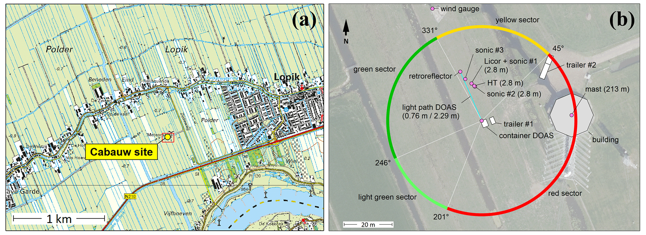
Figure 1The area surrounding the Cabauw measurement site (a). Cabauw is in a flat area at −1 m, in the delta of the river Lek shown in the south east. The line with housing going east-west and running north of the site has a series of farms. Map from https://www.pdok.nl/ (downloaded 7 February 2021). The locations of the instruments (b). The coloured circle denotes wind origin sectors which are used for filtering data (see text). The green and light green sectors indicate wind directions with minimally obstructed flow. Wind from the yellow sector is somewhat obstructed. Wind from the red sector experiences severe obstruction due to the building at the foot of the tall mast, the trailers and the DOAS container. Background aerial photo from https://opendata.beeldmateriaal.nl/ (downloaded 22 February 2022). Data of sonic #3 were not used in the final analysis.
2.2 Instruments overview
For this campaign, the following instruments were set up in a field next to the 213 m mast at Cabauw. The two miniDOAS NH3 instruments were placed above each other in a small container (see below for a detailed description of these instruments). The 22.1 m optical paths were directed at 336∘, parallel to the ditches between the fields. The bottom path was at 0.76 m and the top path 2.29 m above the field. Anticipating prevailing winds from the south-west, the other instruments were positioned 3 m east of the miniDOAS optical paths (Fig. 1), to minimise distortion of the incoming airflow. The instruments each integrated spectra during 4 min and provided simultaneous path-averaged concentration values at 4 min intervals. These concentrations were then averaged to 30 min values. The HT8700E OP NH3 analyser (see below for a detailed description of this instrument; hereafter referred to as “HT”), was mounted on a steel mast with the centre of its optical path at 2.80 m above the ground. On a second steel mast, 1.5 m from the first, a sonic anemometer (sonic #1; model Gill WindMasterPro™, Gill Instruments, Lymington, UK) was mounted. This sonic measured the 3D wind components at 32 Hz 2.8 m above the ground. The 10 Hz OP H2O and CO2 analyser (LI-7500DS, LI-COR Biosciences, Lincoln, USA) was placed at 2.83 m above the ground next to sonic #1.
From 30 September onwards, to evaluate the impact of sensor separation between the HT and the sonic #1 on the calculated NH3 fluxes, a second sonic anemometer (sonic #2, model Gill WindMaster™, Gill Instruments, Lymington, UK) measuring at 32 Hz was installed 40 cm from the HT analyser.
In Fig. 1 we show different coloured wind sectors. The selection is based on objects on the site that influenced the wind field and thus the flux intercomparison. The four wind sectors (Fig. 1) were:
- a.
The green sector (246–331∘): minimal disruption. Only the drainage ditches are expected to influence the wind field.
- b.
The light green sector (201–246∘): minimal disruption. We expected the DOAS container to have some influence.
- c.
The yellow sector (331–45∘): some disruption. The masts with HT and the sonics disturbed the wind field at the DOAS paths. At times, the sheep farmer positioned a small trailer there on the field to the north of the 213 m mast, and sheep were grazing there. This would have affected all instruments.
- d.
The red sector (45–201∘): severe disruption. The 213 m mast, the building at the foot of this mast, the trailers and the DOAS container all affected all instruments.
2.3 Weather conditions
Historically, winds from the southwest tend to be most common in September. During the campaign, the weather was slightly warmer and substantially drier than normal for this time of year (Homan, 2021) (Fig. S4). However, there were no extremely hot or cold spells. No significant precipitation occurred during the measurement period, except for a few short shower events in late September. The wind direction during the campaign was variable and therefore different from the expected predominant wind direction.
3.1 Aerodynamic gradient method (AGM) NH3 fluxes
3.1.1 MiniDOAS instruments
Differential optical absorption spectroscopy (DOAS) is an optical technique to measure trace gas concentrations over an OP in the atmosphere (e.g. Platt and Stutz, 2008). For this experiment, two identical RIVM miniDOAS 2.2D instruments were used. These are active DOAS systems, i.e. equipped with their own light source rather than using sunlight. The light is sent to a retroreflector over an open path of 22.1 m and received back (Fig. 3). Path-averaged NH3 concentrations are retrieved from spectra taken in the 200–230 nm wavelength range.
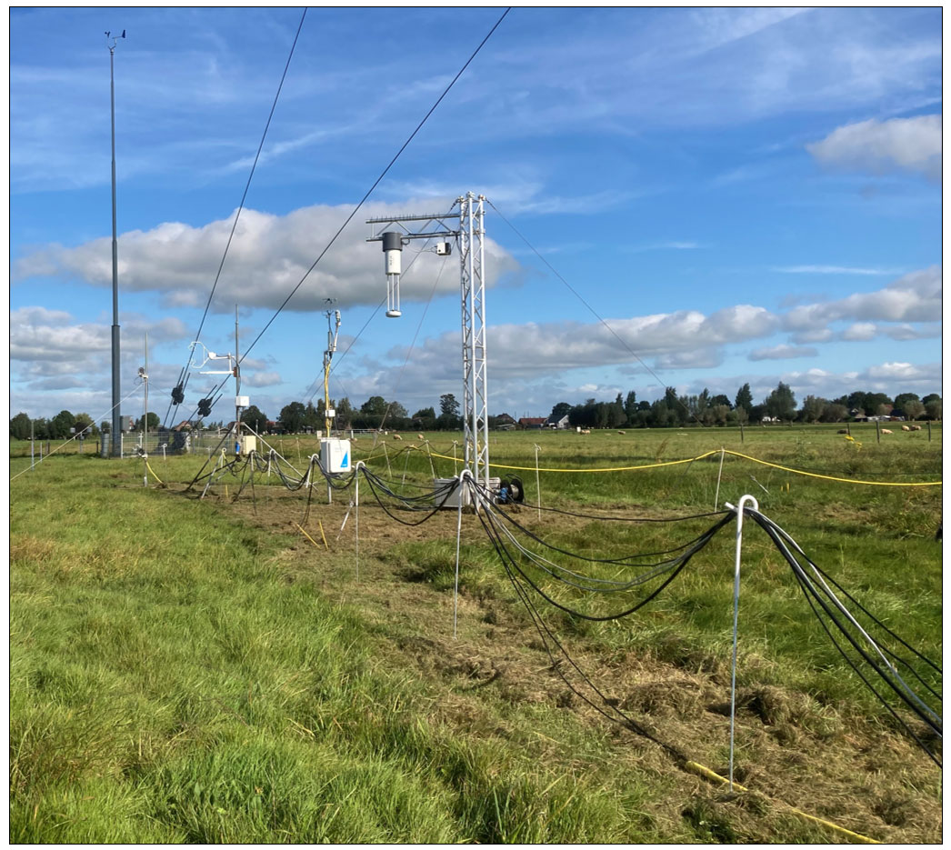
Figure 2The instruments seen from the miniDOAS container looking north. From left to right: 10 m wind gauge mast, mast with the two retroreflectors of the miniDOAS instruments, mast with sonic #3, mast with sonic #1 and LI-7500DS, mast with HT8700E and its cooling unit. Sonic#2 was placed later at 40 cm on the southeast side of HT8700E on the same mast (not shown in the photo). The 213 m mast is off to the right (east).
The 2.2D instruments are a modified and further developed version of the miniDOAS 1.x described earlier (Berkhout et al., 2017; Volten et al., 2012b). MiniDOAS 1.x instruments have been operating in the Dutch national air quality monitoring network since 2016 at 6 locations. The uptime of these instruments in 2021 was above 95 % of the hourly values.
Improvements in the 2.2D version include the use of a more sensitive charge-coupled device detector and several optical components with higher reflectivity and/or transmission in the wavelength range used, leading to an increase in optical throughput by about a factor of 5. The optical layout was simplified and an optical scanner was added, making the system less sensitive to small alignment changes. These modifications resulted in a substantial increase in precision and stability of the measurements as was needed for the monitoring of dry NH3 fluxes with the AGM method. We aim to describe the miniDOAS 2.x in more detail in a forthcoming publication, in combination with the implementation of this version in the Dutch national air quality monitoring network LML.
3.1.2 MiniDOAS calibration and intercalibration
As the AGM method depends on the ability to measure small concentration differences between two heights, great care must be taken to calibrate the two miniDOAS instruments properly, first individually and then as a pair, and to maintain this calibration over the flux measurement period. This process is described below.

Figure 3MiniDOAS set-up in the field, using two instruments at different heights above the ground. The NH3 flux is determined from the observed concentration difference between the top and bottom paths and the turbulence measurements of sonic #1 (flux period, shown in purple). Shown in green are the two instruments in cross-position (cross period). These zero-difference measurements are used for the precise intercalibration needed for flux measurements (see text).
Initial individual laboratory calibration
Each instrument was calibrated according to the procedures used in the LML network. This included the acquisition of a reference spectrum with known, preferably zero concentrations of NH3, SO2 and NO. For this, the zero-tunnel calibration facility at RIVM was used. This spectrum served as a common reference for all measurements. We also acquired calibration spectra of the three gases mentioned, using a flow cell in the light path in combination with the zero-tunnel facility. These spectra contain the spectral fingerprint and cross-section of these gases used in the analysis. For this step, calibration gases of these components with a supplier-indicated accuracy of 2 % were used.
Afterwards, the accuracy of the NH3 calibration was tested by providing two NH3 mixtures in N2 from certified reference cylinders, representing a low and a high concentration of about 35 and 350 µg m−3 in the atmosphere, respectively (Certified Reference Materials, produced by the Dutch National Metrology Institute VSL). These reference cylinders have a certified accuracy of 3 % and 2 % respectively. The instrument calibration was considered valid if the measurement result was within 3 % of the certified reference.
Additional intercalibration for deposition
While suited for concentration monitoring, the calibration approach above is not precise enough for AGM, where concentration differences of 0.1 µg m−3 or better need to be determined, i.e. well below the 1 % level. For this, an additional calibration of the two miniDOAS instruments is needed as a pair. This was done after installation in the field.
The instruments were manually set to a different alignment position, as indicated in Fig. 3, the so-called cross-position. As both instruments now sample on average the same height region, results should be identical for all flow situations where the NH3 gradient is homogeneous over the horizontal path. In this cross-setting, the instruments were set to run for several days, until a sufficient amount of variation in outside air concentrations were encountered. Typically, the intercalibration lasts at least 3 d under suitable conditions.
First, new simultaneous reference spectra for both instruments were obtained from the dataset obtained during the intercalibration to replace the reference spectra obtained in the zero-tunnel. The obtained absolute concentration values from these spectra will be less accurate, i.e. they may have a small but fixed offset to the laboratory values. They will, however, be more precise which is essential for gradient measurements. Next, the spectra obtained in the cross period were processed with these new reference spectra
When comparing the results from both instruments in a scatter plot, the minor additional corrections to the offset and span can be obtained that are needed to make the instruments match perfectly, with offset 0 and slope 1.
The Results section (Sect. 4.1) illustrates that after these steps the pair of instruments was capable of measuring NH3 differences within our target precision of 0.1 µg m−3. The new field reference spectra and the small additional corrections obtained in the cross-position are kept and also applied in the analysis of the flux measurements obtained in the parallel position.
3.1.3 Flux calculation
The 30 min concentration measurements obtained at the 2 measurement heights were combined with 30 min averaged transfer velocities to obtain the AGM NH3 flux FAGM (e.g. Trebs et al., 2021):
where u∗ is the friction velocity, k is the Von Kármán constant (0.4), is the NH3 concentration at height zn, z1 and z2 are the heights of the bottom and top miniDOAS paths above the displacement height d (assumed to be 2/3 of the canopy height), respectively, is the integrated stability function for heat, which is assumed to be the same for NH3 and L is the Monin-Obukhov length. For unstable conditions (L<0), we used the functions of Dyer (1974) and Paulson (1970). For stable conditions (L>0), we used the function of Beljaars and Holtslag (1991). The micrometeorological parameters u∗ and L were calculated using EddyPro software (LI-COR Biosciences) using data collected by sonic #1. The AGM fluxes were calculated using custom software written in R. We follow the sign convention where positive fluxes indicate emissions and negative fluxes deposition.
3.2 Eddy covariance (EC) NH3 fluxes
3.2.1 HT8700E instrument
The OP QCL-based NH3 analyser (Healthy Photon Lt. Co., Ningbo, China, Model HT8700E; hereafter HT) was used to measure NH3 concentrations at 10 Hz using the wavelength modulation spectroscopy technique. Technical details of the analyser have been described in Wang et al. (2021). The QCL sends a beam at 9.06 µm into an open-air Herriott cell which has two concave mirrors of high purity molybdenum with a coating that should withstand frequent cleaning with organic detergents. The temperature of the QCL and detectors are stabilised by Peltier thermoelectrical coolers (TEC). The analyser is coupled to a compact external water and ethylene glycol chiller (Wang et al., 2021).
The HT8700 performance in laboratory and field experiments has been presented by Wang et al. (2021, 2022). The uncertainty of the NH3 concentration measurements was estimated to be ±15 % by comparing two commercially available high-sensitivity NH3 analysers G2103 (Picarro Inc., Sunnyvale, USA) and EAA-911 (Los Gatos Research, LGR, San Jose, USA) in the laboratory (Wang et al., 2021). In the follow-up study (Wang et al., 2022) a slightly higher noise ratio (0.41±0.06 ppbv) and flux detection limit (9.6±1.5 µg N m−2 h−1, equivalent to 3.2±0.5 ng NH3 m−2 s−1) were found after 1-month long monitoring at a wheat field in Northern China.
Raindrops, dust, and other contaminants on the mirrors (particularly the bottom one) cause light scattering which is shown in the optical signal strength (OSS) of the HT (Wang et al., 2021). In contrast to Wang et al. (2021, 2022) in this experiment we used an upgraded HT version equipped with an automated mirror cleaning system (the SPIDER®) that can be activated remotely, which significantly reduced the manual cleaning burden. During this campaign whenever the OSS value dropped below 40 % the lower mirror was cleaned using the SPIDER® for 1–2 min at a time. In addition, both mirrors were manually cleaned 1–2 times per week using lens tissue drenched in methanol if automatic cleaning was not sufficient. However, the OSS values gradually decreased over the experimental period especially after multiple rain events before the end of the campaign (Fig. S5).
3.2.2 Flux calculation
The EC NH3 fluxes and other micrometeorological parameters were calculated using EddyPro software (LI-COR Biosciences) at 30-min intervals using the 10 Hz raw data. The general flux calculation procedure followed the standard FluxNet methodology (Mcdermitt et al., 2011) and some basic settings following Wang et al. (2021). For detailed settings and parameters of this study see Table S1. In addition to the analysis in EddyPro, additional spectral analyses were further tested to study the impact of high-frequency spectral damping and sensor separation on the flux results.
High-frequency spectral losses correction
The eddy flux method evaluates the vertical transport of gas, heat or momentum caused by a composition of turbulent eddies that cover the spectrum from cm to km scale or, in the time domain, from 10 Hz to 30 min scale. Measured EC fluxes correlate the vertical wind and the concentration variation, the covariance of which can be visualised in a cospectrum showing the contribution of the large and small turbulent motions. The raw measurement data need corrections for turbulence-spectral losses both in the low-frequency (> minutes) and high-frequency (> 1 Hz) ranges. For the OP system, the former is caused by the finite averaging time, as the measurement system will not “see” large scale eddies that take longer than the 30 min evaluation interval. The concentration changes that occur with a high frequency (linked to small eddies) are dampened due to the sensing volume of the instrument (which is 50 cm high and will not show eddies that are 10 or 5 cm in diameter) and due to the spatial separation between sonic anemometer and gas analyser (Moore, 1986).
Using the EddyPro software low-frequency flux losses were corrected according to Moncrieff et al. (2004). For estimating high-frequency flux losses the theoretical method from EddyPro (hereafter referred to as TEO; Moncrieff et al., 1997) was applied first. Two remarks have been made on this procedure. First, a difference can occur between the measured cospectra and the theoretical frequency distribution of Kaimal cospectra (Kaimal et al., 1972; Moncrieff et al., 1997). Second, in EddyPro's implementation of the method of Moncrieff et al. (1997) the correction for sensor separation is independent of the wind direction, which holds as long as the distance between the sonic anemometer and gas analyser is relatively small (Moore, 1986). Moore (1986) already indicated that in doing so the flux correction would probably be overestimated. Therefore, to better understand the real field condition and equipment separation results in EC flux, an empirical approach using measured gas flux cospectra and sensible heat cospectra as references was applied similar to Wintjen et al. (2020, hereafter referred to as in situ cospectral method, ICO). For detailed ICO method data quality control, see Sect. 1.1 in the Supplement.
Modified WPL correction
Open-path trace gas concentrations are affected by density variations in the upgoing and downgoing air movements. The Webb, Pearman and Leuning (WPL) correction accounts for that (Webb et al., 1980). Two WPL methods were used. First, the classical WPL method was used to correct H2O measurements from LI-7500DS. Apart from that the NH3 flux is also affected by spectroscopic effects (Burba et al., 2019). The spectroscopic part is instrument-dependent and deals with the effect of changing H2O concentrations and their impact on the absorption line used for NH3. Hence, the modified WPL method was applied to correct the HT-measured NH3 flux following Wang et al. (2021):
where ρA is the NH3 density corrected for temperature (see Sect. 4.1.2), ρd is the dry air density, ρv is the water vapour density, μ is the molar mass ratio of dry air to water vapour, is the water vapour flux measured by the LI-7500DS, Ta is the air temperature and is the sensible heat flux from the sonic anemometer. A, B, and C are dimensionless parameters accounting for the spectroscopic effects from Wang et al. (2021), which vary with ambient temperature, pressure and water vapour content.
3.3 Quality control and filtering
Firstly, observations from the HT were filtered out before the EC flux analysis if the optical signal strength (OSS) of the NH3 analyser was below 40 % (Fig. S5). Secondly, after EC analysis in EddyPro was completed, EC fluxes were removed if a quality flag of 2 was assigned according to the stationarity and integral turbulence tests proposed by Mauder and Foken (2006). Thirdly, both fluxes with u∗ values smaller than 0.1 m s−1 were discarded to filter out observations during low-turbulence mixing conditions. Fourthly, a moving window outlier filter was applied to the remaining fluxes, removing points if two times the standard deviation of the adjacent six flux values was exceeded (Wang et al., 2021, 2022). Finally, the data were grouped into four different wind sectors (green, light green, yellow and red) as described in Fig. 1. Only observations from the green and light green sectors were used for the intercomparison of the fluxes. An overview of the applied filters and the percentage of accepted fluxes per filter step are shown in Table S2.
3.4 Uncertainty analysis
A description of the random error analysis of the half-hourly AGM and EC fluxes is given in Sect. 1.2 of the Supplement.
3.5 Footprint analysis
The footprint of the EC fluxes showing the contributing area of measured fluxes was analysed following the method from Kljun et al. (2015a). Inputs for this method include the EC measurement height (z=2.80 m), roughness length (assumed to be 0.15 times canopy height), friction velocity (u∗), the Obukhov length, the standard deviation of the lateral wind (v) component, wind direction, mean wind speed, and the boundary layer height. Apart from the boundary layer height, other parameters were measured by the EC system. The hourly boundary layer height data was obtained from Climate Data Store (CDS) (Hersbach et al., 2018) and the hourly values were linearly interpolated to half hourly values for the footprint calculation. The flux footprint prediction (FFP) method (Kljun et al., 2015b) was used for coding and plotting. Here, footprints were only determined for EC NH3 flux after quality filtering (see Sect. 3.3). No separate footprint analysis was done for the AGM fluxes.
4.1 NH3 concentrations
4.1.1 MiniDOAS intercalibration
The laboratory calibration procedure of both individual miniDOAS instruments is described in the instrument section (Sect. 3.1.2). Here, the result of the intercalibration in the field is shown, which aims to increase the precision of the concentration difference measurement further. Intercalibration measurements were taken in three periods: at the beginning and end of the campaign and once during the campaign. In total, 35 % of the 7-week uptime was spent on intercalibration. The data were filtered for well-mixed situations ( and obstacle-free wind directions (green and light green) in order to obtain homogeneous concentration gradients along the path. Figure 4 shows a scatter plot of the obtained concentration measurements by both instruments matching these requirements.
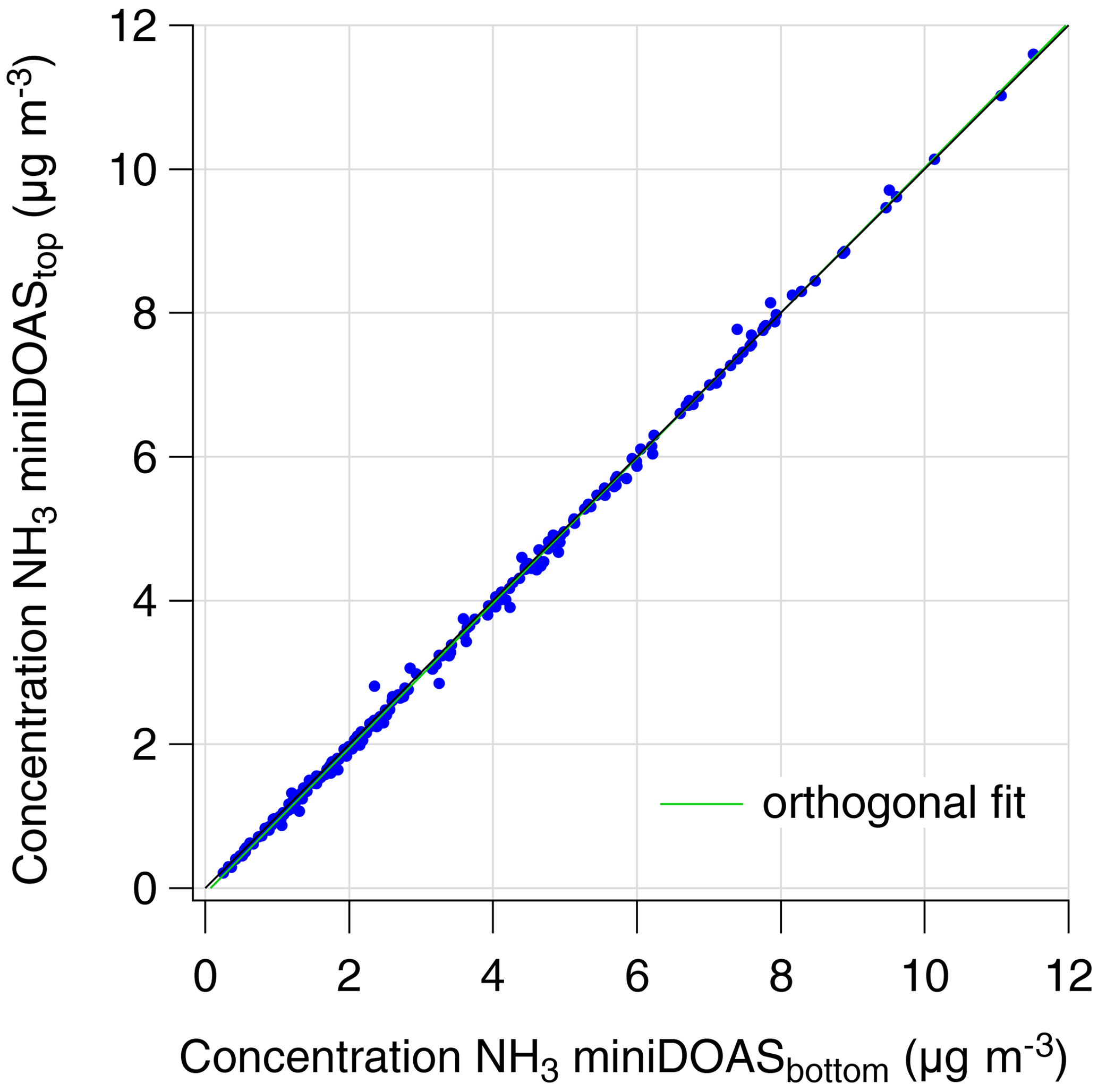
Figure 4Scatter plot of data obtained by the two miniDOAS instruments during all three cross-periods. Data were filtered to include only obstacle-free wind directions and turbulent conditions ( m s−1). Using an orthogonal fit, an offset of 0.07±0.01 µg m−3 and a slope of 1.009±0.002 (the green line) were found.
The offset and slope corrections were applied to the concentrations of miniDOAStop over the full campaign. The standard deviation of the residuals was used as an estimate of the remaining random uncertainty in the concentration difference after correction. This random error was determined to be 0.088 µg m−3.
The results of the intercalibration periods are discussed in Sect. S1.3. The conclusion is that over the full campaign period, the zero level of the difference measurement has been stable, and the individual difference measurements showed a typical spread of 0.1 µg m−3 or less.
4.1.2 HT concentration corrections
The HT NH3 concentration measurement contained a considerable number of gaps in the data (21 % during the 5-week uptime). These gaps largely occurred during rain and mirror cleaning afterwards. At the start of the campaign, the HT instrument had an offset of about −7 µg m−3 (data not shown). After the campaign, the analyser was recalibrated in the laboratory and the “zero” was found to be µg m−3 when flushing pure nitrogen gas for 6 h through the calibration cell while the temperature was kept constant at 17 ∘C. Before temperature correction the raw HT and miniDOAStop's average difference was −5.3 µg m−3 (range −15 to 6 µg m−3, n=1180) during the overlapping period of the campaign. The raw half hourly HT NH3 concentrations showed inconsistent differences compared to the miniDOAS concentration levels, which varied with air temperature. After applying a third-order polynomial fit of the HT-miniDOAS concentration difference versus temperature, the corrected concentrations for HT were finally obtained (Fig. S7). Temperature mainly impacted on the offset of its concentration and it seemed to have a negligible influence on the span of the HT concentration (slope ≈ 0.97, Fig. 5).
4.1.3 Comparison of miniDOAS and HT concentrations
After application of the temperature correction on the NH3 concentrations of the HT, the concentrations from the two instruments were very similar (R2=0.97, Fig. 5). Furthermore, the time series of the corrected NH3 concentrations from both instruments captured the same temporal pattern and peak events. The highest concentrations were observed during nighttime when the boundary layer height is small and vertical mixing is limited. During daytime the concentrations decreased due to the rise of the boundary layer and the increased vertical turbulent transport (Fig. 6).

Figure 5Scatter plot of the NH3 concentrations from the miniDOAStop and the temperature-corrected HT instrument during parallel measurements (correlation line was forced through the origin).

Figure 6Time series of the measured unfiltered NH3 concentrations after temperature correction from the HT (red) and the miniDOAS instruments (dark blue for miniDOASbottom; light blue for miniDOAStop in µg m−3, the hourly ambient temperature (black) in ∘C and the amount of rainfall (grey bars) in mm.
4.2 Uptime, filtering and quality control
For the AGM method the vertical NH3 concentration gradient measured by the miniDOAS instruments and the transfer velocity from the sonic #1 anemometer were used to determine the NH3 flux. Figure S8a shows the full time series of the NH3 flux derived using the miniDOAS set-up. The miniDOAS set-up had an uptime of nearly 100 % over the full campaign (1142 h). Except for the 35 % intercalibration periods, 80 % of the remaining parallel measurements (597 h) were left after filtering out low turbulent mixing conditions ( m s−1) and outliers. For the EC NH3 flux measurements, Fig. S8b shows the full time series. The uptime of the HT instrument was 79 % during the 5-week field operational period (685 h). After filtering for fluxes with poor quality flags, m s−1 and outliers, 59 % of the valid observations remained (516 h). Observations on the 11 September were excluded due to large differences between the measured fluxes on that day, although they originated from green wind directions. We assume this was related to manuring at the adjacent field that might have disturbed the footprint homogeneity of the flux but we have no evidence to support that. After filtering, 848 overlapping half hours were left for flux comparison between two instruments.
4.3 Comparison of the AGM and EC fluxes
Both NH3 fluxes are shown in Fig. 7. Here, the EC fluxes corrected for flux damping in EddyPro are shown, which is considered as a reference method. After quality control filtering, the EC and AGM fluxes have a similar range and pattern. Within the green and light green sectors, the highest NH3 emission measured with the AGM set-up was 0.18 µg m−2 s−1 and deposition was 0.15 µg m−2 s−1. The highest observed NH3 emission with the EC set-up was 0.16 µg m−2 s−1 and deposition was 0.10 µg m−2 s−1.
At the start of the measurement period, the AGM and EC fluxes were quite different. During the first days, the miniDOAS system presented NH3 deposition, while the HT showed NH3 emissions. In this period, the prevailing winds were from the north and northeast, categorised as yellow (see Fig. 1), where sheep were occasionally located upwind of the instruments. This may have caused inhomogeneity in the pattern of sources and sinks within the footprint area (see below), which would have violated the AGM and EC calculation assumptions. Furthermore, the NH3 concentrations during this episode were relatively high as manuring activities were still allowed until 15 September on the grasslands surrounding the measurement site. In the green and light green wind directions, the NH3 fluxes from the two methods compared well after 20 September when little or no effect of manure application should be present.
Considering only high-quality measured fluxes during this period, the cumulative daily fluxes of the AGM and EC were in general similar, with typical differences in the order of ∼ 10 % (Fig. S9). When looking at the cumulative flux over the full period, however, a larger difference was observed. This difference appeared stepwise on a single day, 24 September. On this day, and only during a few hours around noon, there was a much larger flux observed by EC compared to AGM. Most likely, the discrepancy was caused by footprint issues in combination with very local emissions. Unfortunately, we lack the means to validate this assumption.

Figure 7Time series of the NH3 fluxes of AGM with miniDOAS instruments (blue) and the EC method from the HT (red). Positive fluxes indicate emissions, negative fluxes deposition. The colours in the upper and lower borders indicate the prevailing wind directions from Fig. 1. The intercalibration periods for the miniDOAS instruments are shown against a grey background. The thick lines indicate the NH3 fluxes that were left for intercomparison after all filters were applied.
Figure 8 shows the comparison of the EC (calculated by EddyPro) and AGM NH3 fluxes per categorised wind direction. There was a strong correlation (r=0.87) between the EC and AGM NH3 fluxes at times where the airflow was unobstructed, i.e. when the wind came from the directions categorised as green. In this category the differences between the EC and AGM NH3 fluxes were also relatively small (root mean square error, RMSE = 0.027 µg m−2 s−1, bias = 0.012 µg m−2 s−1). There was a moderate correlation between the EC and AGM NH3 fluxes in the light green (r=0.71) and the red categories (r=0.69). In both the green and light green categories the AGM-based fluxes were approximately 30 % above the EC-based levels (slope = 1.3 for green and slope = 1.35 for light green). In the red category, the airflow was partially obstructed by large objects. In this category, the EC fluxes were generally larger than the AGM fluxes (slope = 0.64), but relatively small differences (RMSE = 0.034 µg m−2 s−1, bias = −0.016 µg m−2 s−1) between the EC and AGM NH3 fluxes were still found. The poorest agreement (r=0.33, RMSE = 0.072 µg m−2 s−1, bias = −0.045 µg m−2 s−1) between the two methods was found for the yellow wind direction category. In this category, the HT often observed NH3 emissions while the miniDOAS set-up observed deposition of NH3.

Figure 8Comparison of the AGM NH3 fluxes from the miniDOAS instruments and the EC NH3 fluxes from the HT per colour-categorised wind direction (see Fig. 1).
The two methods showed a similar diurnal pattern using NH3 fluxes from the green and light green wind directions (Fig. 9). NH3 was generally emitted during the day and deposited during the night. Between 10:00 and 14:00 UTC, the AGM fluxes were a factor of ∼ 1.7 higher than the EC fluxes. Figure S10 in the Supplement shows the diurnal pattern using only data after 15 September. The midday differences between the two are smaller, but still exist, even though manure spreading was not allowed anymore.
4.4 Uncertainty analysis
Figure 10 shows the random errors of the AGM and EC NH3 fluxes and the contribution of different components to the error. The random errors of the two showed a similar range of values. On average, EC NH3 fluxes had a slightly lower error. The mean random error (1σ) of the AGM NH3 flux was 15.0 ng m−2 s−1 (median 7.4 ng m−2 s−1), while the mean random error of the EC NH3 fluxes amounted to 5.5 ng m−2 s−1 (median 4.1 ng m−2 s−1). The mean and median relative random errors were 89 % and 24 % for the AGM flux versus 61 % and 15 % for the EC flux, respectively.
The random errors of the AGM fluxes showed a clear diurnal pattern. During the daytime, the random errors were relatively large and peaked around noon, because the observed gradient was the smallest at this time. As a result, the measurement error in the NH3 concentration differences dominated. During the night, the random errors were relatively small and the errors in the u∗ values had a relatively large contribution. As a consequence, especially deposition estimates were sensitive to the random error in u∗. The largest random errors in the NH3 fluxes largely took place when the error in the stability correction took over, i.e. when a substantial stability correction was applied to the measurement heights of the miniDOAS instruments. This occasionally occurred during nighttime, usually around midnight. Compared to the random error of the AGM NH3 fluxes, the diurnal cycle of the random error in the EC NH3 fluxes was less apparent. The contributions of the heat terms in the WPL correction to the total random error were negligible. The contribution of the error in the WPL water vapour term could be quite substantial (max. ∼ 75 %) in incidental cases but was generally between zero and ∼ 20 % during daytime.

Figure 9Mean diurnal cycle of the EC and AGM NH3 fluxes. Positive flux is emission, negative flux is deposition. The error bars indicate the standard error of the hourly means . The number of hours averaged are listed in blue text at the top. Here, filtered NH3 fluxes from only the green and light green wind directions where both systems have a valid flux observation were used. Data from the 11 September are also excluded due to a potential emission event causing footprint heterogeneity.
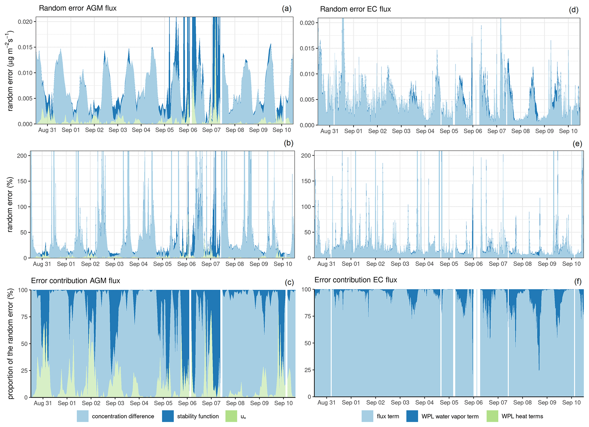
Figure 10The random error in µg m−2 s−1 (a, d), random error in % (b, e) and proportion of the random error in % (c, f) of the AGM (a, b, c) and EC (d, e, f) NH3 fluxes from 31 August to 10 September. For the EC fluxes, the light blue component (flux term) refers to F1 in Eq. (S2) in the Supplement, based on fluxes determined using EddyPro, taking into account the damping correction and term A from Eq. (2).
4.5 Footprint analysis
The footprint of the EC NH3 fluxes was computed at sonic #1 height using the method from Kljun et al. (2015a) and shown in Fig. 11a for all wind directions and in Fig. 11b for only the green and light green sectors. Overall, 80 % of the flux originated from an area within approximately 100 m distance from the measurement devices. Furthermore, the influence of the 213 m mast seems visible and reduces the footprint to the southeast. Because the highest measurement point has the largest footprint, the footprint of the miniDOAS instruments, especially miniDOASbottom, will be substantially smaller. The measured fluxes are assumed to be representative of the footprint area. The largest footprint area determines the outside perimeter of the area within which the landscape should be homogeneous. If that is not the case it can be expected that the AGM and EC methods will end up with different results.
4.6 Damping correction methods: TEO versus ICO for EC flux
To evaluate the effect of damping on the EC flux, both the theoretical method from EddyPro (TEO) and the empirical method (ICO) were used. In the results above we used the EddyPro theoretical approach (Table S1) as we considered that as the standard evaluation method. The comparison showed that TEO corrections were larger than the ICO factors for CO2, H2O, and NH3 (Fig. S11). The sensible heat flux cospectrum indicated that the Kaimal cospectrum in TEO did not represent the turbulent characteristics of the site well enough (Fig. S12). Application of the ICO method on the HT data, however, decreased correlations with the AGM results in the light green and green wind sectors (Fig. S13). The ICO method seems to be conceptually better. However, ∼ 50 % of the dataset had to be corrected using daily median values because the measurement-based ogives were noisy (caused by low flux conditions). We therefore decided for this relatively short campaign to still use the TEO method for the flux comparison with the AGM method.
The damping is affected by both the sensor separation and the sensing volume. The HT and the combination of sonic #1 and LI-7500DS were 1.5 m apart during the entire campaign period. Using sonic #1 data, the HT instrument median flux damping of NH3, CO2, and H2O were 37 %, 1 %, and 1 %, respectively, according to the ICO method. Data from sonic #2 which was installed at the end of the campaign for 2 d at 0.40 m distance to the HT and 1.35 m to the LI-7500DS ICO gave 16 %, 32 %, and 31 % for NH3, CO2, H2O damping, respectively. So the separation between the HT and sonic #1 caused ca. 20 % extra damping for NH3 fluxes. Separating the LI-7500DS and sonic #2 by the same distance caused 30 % damping for the H2O and CO2 fluxes. That could be explained because the HT has a 4 times longer vertical path length than the LI-7500DS sensor (0.50 m vs. 0.125 m) in which higher frequencies will be damped anyway.
The TEO method, applied for the 2 d with both sonics available, gave median damping factors 41 %, 14 % and 14 % for NH3, CO2, and H2O, respectively, using sonic #1 and 20 %, 38 %, and 37 %, respectively, using sonic #2. Both TEO and ICO methods produced the same damping difference between the two sonics for NH3 flux (ca. 20 %). As a consequence, the corrected NH3 fluxes obtained with sonic #1 or sonic #2 were the same (see Fig. S14) suggesting the damping correction provides reasonable flux estimates. When comparing the fluxes with sonic #1 during the entire campaign period, the TEO corrections for all gases were larger than the ICO ones (see Fig. S11). For NH3 flux losses were 39 % versus 28 %, respectively. Surprisingly, even without extra distance separation between LI-7500DS and sonic #1, TEO suggests 12 % correction for the H2O and CO2 flux while ICO only suggests 2 %–3 % damping correction as average for the entire period.
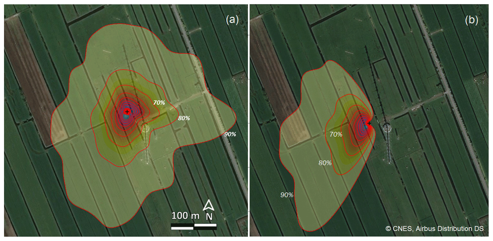
Figure 11Footprint climatology estimate of the EC measurements (z=2.8 m) for (a) all wind sectors and (b) the green and light green wind sectors. The red curves are at 10 % footprint contour lines. Background map data: Microsoft, CNES Distribution Airbus DS.
We had the unique opportunity to use two newly developed OP instruments providing independent data for the NH3 flux estimates. An overview of the main findings of the 5-week intercomparison campaign can be found in Table 1.
Table 1Overview of the main differences, strengths and weaknesses of the two instrument set-ups compared.
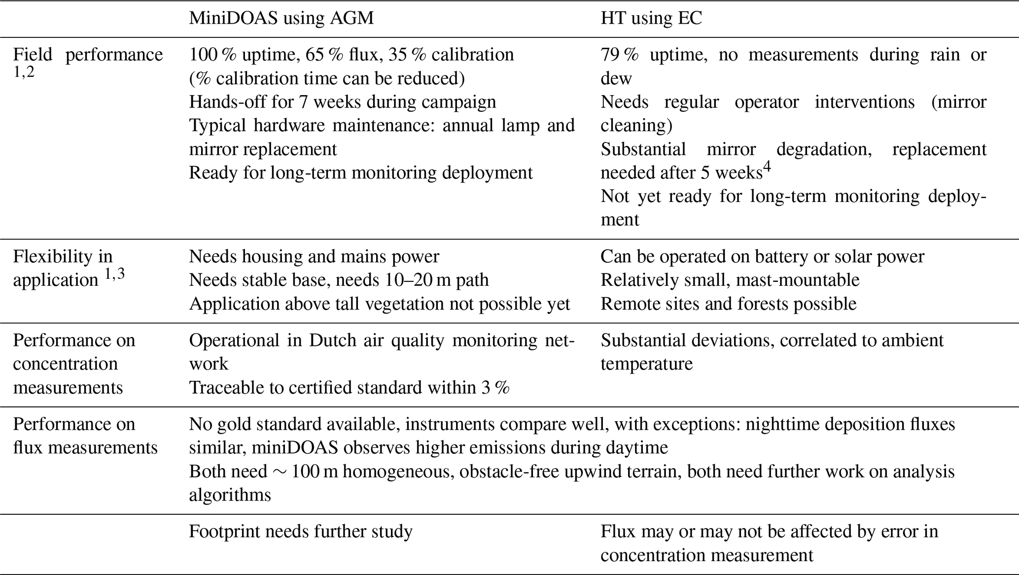
1 More details are given in 2 Sect. 1.4.1 and 3 Sect. 1.4.2. of the Supplement. 4 A more durable mirror is available now.
5.1 Concentration comparison
A substantial and varying discrepancy in NH3 concentrations was found between the HT and the miniDOAS. The miniDOAS instrument is currently used for concentration monitoring in the Netherlands and has a validated accuracy of better than 3 %. Therefore, we concluded that the observed discrepancy was caused by a substantial and varying offset in the HT concentrations, which correlated with the changing ambient air temperature (Fig. S7, Earlier, Wang et al. (2021) compared measured NH3 concentrations of the HT to those of a Picarro instrument during a 14 h experimental period. The differences were within 10 %. However, the indoor air temperature during that relatively short experiment would likely have been fairly stable, so any impact of temperature on HT concentration measurements could easily go undetected. Reliable measurements of the absolute concentration are especially important for flux interpretation beyond the net flux, and also when calculating deposition velocities. It is therefore important to improve the accuracy of measured concentrations of the HT itself.
5.2 Flux comparison
The overall pattern of the fluxes and the diurnal cycles agreed remarkably well between the DOAS-AGM and the HT-EC set-ups when the wind came from the green sectors, where upwind terrain was relatively homogeneous and obstacle free. Larger differences were observed for the other wind directions (Fig. 10). These discrepancies can have several causes.
Firstly, obstacles in the terrain upwind may interfere with both measurement techniques, as they affect atmospheric turbulence patterns and disturb the NH3 gradient. All instruments were influenced by the 213 m high tower (∼ 60 m away), especially when the wind came from the southeast (red wind sector). Here, the correlation between the fluxes, however, was still modest (r=0.69). When the wind blew from the north (yellow wind sector), the agreement between AGM and EC fluxes was poorest (r=0.33). This may indicate that the heterogeneity of the footprint area had a larger influence on the fluxes measured by the two systems. Due to the differences in measurement height and path sampling versus point sampling, the AGM and EC set-ups have different footprints (Loubet et al., 2013). If either the terrain or fluxes were inhomogeneous, the set-ups may therefore have captured different NH3 fluxes. At this site, spatial homogeneity may partly be violated by the ditches in the terrain. Direct emissions may be spatially inhomogeneous due to manure or fertiliser application or excreta from grazing animals. In a follow-up campaign, the comparison of the miniDOAS and the HT instrument should be continued at more homogeneous sites, avoiding nearby obstacles and (animal) emission sources within the footprints.
The substantial deviations in NH3 concentrations from the HT were strongly linked to ambient temperature. In the current analysis, we treated these deviations as a temperature-dependent offset. As ambient temperatures only changed gradually in time, so did the applied offset in the correction. As a consequence, this correction had virtually no impact on the HT flux measurement as the flux measurement is based on observed concentration variations on a short time scale. It is, however, not clear if the effect of temperature is limited to inducing only an offset in concentration. There could also be an influence on the span: at higher temperatures the HT might be more, or less, sensitive to NH3. This would affect the flux measurement by the same factor and could be an explanation for the discrepancy in flux between miniDOAS and HT during daytime (Fig. 9). To eliminate this possible source of discrepancy, further studies on the cause and the exact effect of the temperature on the offset and slope of the HT calibration are necessary.
In this paper, standard flux processing was used for both techniques. Our instrument set-ups, however, were different from regular AGM and EC instruments (path versus point for miniDOAS, larger measurement volume for HT) and we were dealing with a new gas. These analysis techniques may therefore need adaptations. For example, we tested different damping methods and found different flux results. The theoretical damping correction (TEO) of Moncrieff et al. (1997) added about 40 % to the raw flux. When using the empirical (ICO) method (Wintjen et al., 2020), however, the damping effect was estimated to be only 30 %. As we do not have a very large dataset and because the empirical method can only properly run on the subset of the data that has fluxes large enough to make a reasonable spectral distribution, the fit of miniDOAS vs. HT when using ICO shows more scatter (Fig. S13). We therefore chose to present the comparison based on the TEO correction, a method that is always available as it relies only on the arrangement and dimensions of the instrument. However, we strongly advise further evaluation of the damping calculation method. Similar advice is given for the AGM method, where we used the standard stability correction functions which bring a generalisation that might be not fully representative at our measurement site.
We compared two novel open-path optical instruments to measure NH3 concentration and flux during a 5-week comparison period at Cabauw, the Netherlands: two active custom-designed broadband UV-based miniDOAS (differential optical absorption spectroscopy) instruments and a commercially available infrared-based quantum cascade laser HT8700E gas analyser developed by the company Healthy Photon (HT). Both instruments avoid the hysteresis effects caused by the stickiness of NH3 to tubing and instrument interiors, and are as such insensitive to interference by ammonium aerosols. Both instruments showed good uptime during the campaign. The uptime of the miniDOAS system reached 100 % once operational, but regular intercalibration of the two instruments was applied to test baseline stability (35 % of the 7-week uptime). Intercalibration time can be reduced in future applications based on the results of this campaign. The HT does not measure during rain, or shortly after rain while the instrument is drying, causing 21 % data loss over the 5-week campaign. In addition, the coating of HT mirrors tended to substantially degrade.
The miniDOAS system measured fluxes using the aerodynamic gradient method (AGM), the HT8700E measured fluxes using the eddy covariance method (EC). After data quality filtering a total of 848 simultaneous half hourly flux measurements were compared, showing that both instruments gave similar values for the NH3 exchange ranging from ca. −80 to +140 ng NH3 m−2 s−1 (Fig. 7). When the upwind terrain was both homogeneous and free of nearby obstacles within around 100 m, the two systems showed the strongest correlation (n=113, r=0.87) and provided similar temporal patterns. In addition, the observed diurnal pattern of the two systems had the same shape (Fig. 9). As such, the deposition flux during nighttime was ca. 25 ng NH3 m−2 s−1 (equivalent to 465 mol NH3 ha−1 yr−1). The highest emission occurred around noon and was up to 50 ng NH3 m−2 s−1. Moreover, the AGM flux values were larger than the EC ones during daytime.
The uncertainty analysis showed that the random error of the two systems was similar (Fig. 10). The median relative random errors were 23 % for the AGM flux versus 15 % for the EC flux. The median random error (1σ) for half hourly flux values of the miniDOAS was about 7.4 ng NH3 m−2 s−1, and its maximum value generally did not exceed 15 ng m−2 s−1. For the HT, the median and maximum random errors were 4.1 and 10 ng NH3 m−2 s−1, respectively. These values are adequate to allow the study of deposition and emission processes. The random errors of both techniques varied substantially with meteorological conditions and time of day. For AGM flux, it was relatively higher during daytime. The diurnal cycle in the random error of the EC was, on the other hand, far less distinct.
While flux measurements between HT and miniDOAS in general compared well, we found a substantial variable offset in the HT concentrations. They were sensitive to air temperature, causing substantial differences (range −15 to +6 µg m−3) between the two systems. In this study, we used the miniDOAS as a reference to correct the HT concentration using a temperature-dependent offset and assuming no impact on the span. It should be stressed that these offset corrections only have an impact on the HT concentrations, not (or only very minor) on the HT fluxes. However, a temperature dependency in the span would also affect the HT fluxes. Further studies on the temperature dependence of the HT concentrations are needed to confirm that the span calibration is indeed not impacted by changes in temperature.
The footprint analysis for the EC method showed that measurements were representative of the terrain up to approximately 100 m upwind. In the southeast direction, the footprint size was much smaller due to the meteorological measurement tower, which largely blocked the air flow. The footprint size of the AGM was not analysed but is expected to have a similar shape. Moreover, because of the lower measurement heights, the miniDOAS system is expected to have a smaller footprint, and the footprints of upper and lower paths are substantially different.
Spatial heterogeneous flux patterns need to be avoided in the upwind footprint region as they can influence the result and render interpretation more complicated or even impossible. Also, the 10 % difference found between the theoretical (Moncrieff et al., 1997) and empirical (Wintjen et al., 2020) methods for correcting high-frequency losses of EC fluxes may be related to inhomogeneities in the footprint area as they were not reproduced by theoretical cospectra. In addition, the terrain within all footprints needs to be homogeneous in its vegetation type and roughness. For further intercomparisons, obstacle-free, livestock-free, more homogeneous surroundings are highly recommended.
In deposition studies and parameterisations, reliable concentration and flux values are both needed. The miniDOAS provides both values reliably and appeared to be ready for long-term hands-off monitoring. The HT is presented solely as a flux instrument, and makes no claim to being an accurate monitor for NH3 concentrations yet. In addition, the current system had a limited stand-alone operational time under the prevailing weather conditions.
In this study we demonstrated that the miniDOAS and HT8700 systems provide comparable flux measurements at half hourly time resolution. Under the right circumstances, data from both instruments can facilitate the study of processes behind dry deposition in different ecosystems, allowing better understanding and better parameterisation of these processes in chemical transport models. These observations also enable testing and validation of low-cost deposition measurement systems like the conditional time-averaged gradient (COTAG; Famulari et al., 2010), or inferential deposition networks (e.g. those listed by Walker et al., 2020).
The datasets used in this study are available from the corresponding author upon request (susanna.jonker@rivm.nl, shelley.van.der.graaf@rivm.nl).
The supplement related to this article is available online at: https://doi.org/10.5194/amt-16-529-2023-supplement.
DS, AH, SR and TvG designed the study. DS and AH coordinated the field campaign. DS, SB, RvdH and MH developed and tested the miniDOAS instruments and performed measurements during the campaign. JZ, AH, AF and PvdB performed the EC HT measurements. JZ and PW processed the EC and HT data and determined the EC NH3 flux. SB processed miniDOAS concentration data, and SvdG determined the AGM NH3 flux. Figures were made by SvdG, SB and JZ. DS, AH and SR prepared the manuscript with contributions from JZ, SvdG, and SB. MvZ, RS, PW and TvG reviewed and corrected the draft manuscript.
The contact author has declared that none of the authors has any competing interests.
Publisher's note: Copernicus Publications remains neutral with regard to jurisdictional claims in published maps and institutional affiliations.
This work was carried out partly within the framework of the Dutch Ruisdael program (https://ruisdael-observatory.nl, last access: 20 April 2022) and was part of the annual Ruisdael campaign (RITA-2021). Funding from the Ministry of Agriculture, Nature and Food Quality (LNV) is gratefully acknowledged. We thank the Royal Netherlands Meteorological Institute (KNMI) for site access and assistance during the campaign, especially Arnoud Apituley for coordination and help with site selection. We thank Kai Wang, from the Institute of Atmospheric Physics, Chinese Academy of Sciences, Beijing; and staff from Healthy Photon Lt. Co, especially Yin Wang and Peng Kang, for helpful discussions about data processing of the HT. Furthermore, we thank Daniëlle van Dinther (TNO) for merging various data streams during the campaign. We acknowledge RIVM colleagues Kim Vendel for the preliminary processing of the AGM data at the beginning of the campaign, and Miranda Braam for helping with the uncertainty analysis.
This research has been supported by the Ministerie van Landbouw, Natuur en Voedselkwaliteit (programma Stikstof en Natuur (grant no. P36NAT)).
This paper was edited by Folkert Boersma and reviewed by Albrecht Neftel and one anonymous referee.
Bai, M., Suter, H., Macdonald, B., and Schwenke, G.: Ammonia, methane and nitrous oxide emissions from furrow irrigated cotton crops from two nitrogen fertilisers and application methods, Agr. Forest Meteorol., 303, 108375, https://doi.org/10.1016/j.agrformet.2021.108375, 2021.
Bai, M., Loh, Z., Griffith, D. W. T., Turner, D., Eckard, R., Edis, R., Denmead, O. T., Bryant, G. W., Paton-Walsh, C., Tonini, M., McGinn, S. M., and Chen, D.: Performance of open-path lasers and Fourier transform infrared spectroscopic systems in agriculture emissions research, Atmos. Meas. Tech., 15, 3593–3610, https://doi.org/10.5194/amt-15-3593-2022, 2022.
Beljaars, A. C. M. and Holtslag, A. A. M.: Flux parameterization over land surfaces for atmospheric models, J. Appl. Meteorol., 30, 327–341, https://doi.org/10.1175/1520-0450(1991)030<0327:Fpolsf>2.0.Co;2, 1991.
Berkhout, A. J. C., Swart, D. P. J., Volten, H., Gast, L. F. L., Haaima, M., Verboom, H., Stefess, G., Hafkenscheid, T., and Hoogerbrugge, R.: Replacing the AMOR with the miniDOAS in the ammonia monitoring network in the Netherlands, Atmos. Meas. Tech., 10, 4099–4120, https://doi.org/10.5194/amt-10-4099-2017, 2017.
Bosveld, F. C.: The Cabauw in-situ observational program 2000–present: instruments, calibrations and set-up, Royal Netherlands Meteorological Institute, De Bilt, 79 pp., Technical report TR-384, , 2020.
Bosveld, F. C., Baas, P., Beljaars, A. C. M., Holtslag, A. A. M., de Arellano, J. V.-G., and van de Wiel, B. J. H.: Fifty years of atmospheric boundary-layer research at Cabauw serving weather, air quality and climate, Bound.-Lay. Meteorol., 177, 583–612, https://doi.org/10.1007/s10546-020-00541-w, 2020.
Burba, G., Anderson, T., and Komissarov, A.: Accounting for spectroscopic effects in laser-based open-path eddy covariance flux measurements, Global Change Biol., 25, 2189–2202, https://doi.org/10.1111/gcb.14614, 2019.
Dyer, A. J.: A review of flux-profile relationships, Bound.-Lay. Meteorol., 7, 363–372, https://doi.org/10.1007/BF00240838, 1974.
Erisman, J. W. and Wyers, G. P.: Continuous measurements of surface exchange of SO2 and NH3; Implications for their possible interaction in the deposition process, Atmos. Environ. A, 27, 1937–1949, https://doi.org/10.1016/0960-1686(93)90266-2, 1993.
Erisman, J. W., Galloway, J. N., Dice, N. B., Sutton, M. A., Bleeker, A., Grizzetti, B., Leach, A. M., and Vries, W. D.: Nitrogen: too much of a vital resource, Science Brief. WWF Netherlands, Zeist, The Netherlands, 48 pp., ISBN 978-90-74595-22-3, 2015.
Famulari, D., Fowler, D., Hargreaves, K., Milford, C., Nemitz, E., Sutton, M. A., and Weston, K.: Measuring eddy covariance fluxes of ammonia using tunable diode laser absorption spectroscopy, J. Water Air Soil Pollut. Focus, 4, 151–158, https://doi.org/10.1007/s11267-005-3025-9, 2004.
Famulari, D., Fowler, D., Nemitz, E., Hargreaves, K. J., Storeton-West, R. L., Rutherford, G., Tang, Y. S., Sutton, M. A., and Weston, K. J.: Development of a low-cost system for measuring conditional time-averaged gradients of SO2 and NH3, Environ. Monitor. Assess., 161, 11–27, https://doi.org/10.1007/s10661-008-0723-6, 2010.
Flechard, C. R., Nemitz, E., Smith, R. I., Fowler, D., Vermeulen, A. T., Bleeker, A., Erisman, J. W., Simpson, D., Zhang, L., Tang, Y. S., and Sutton, M. A.: Dry deposition of reactive nitrogen to European ecosystems: a comparison of inferential models across the NitroEurope network, Atmos. Chem. Phys., 11, 2703–2728, https://doi.org/10.5194/acp-11-2703-2011, 2011.
Flesch, T. K., Baron, V. S., Wilson, J. D., Griffith, D. W. T., Basarab, J. A., and Carlson, P. J.: Agricultural gas emissions during the spring thaw: Applying a new measurement technique, Agr. Forest Meteorol., 221, 111–121, https://doi.org/10.1016/j.agrformet.2016.02.010, 2016.
Foken, T.: Micrometeorology, Springer Berlin Heidelberg, 308 pp., https://doi.org/10.1007/978-3-540-74666-9, 2008.
Fowler, D., Coyle, M., Skiba, U., Sutton, M. A., Cape, J. N., Reis, S., Sheppard, L. J., Jenkins, A., Grizzetti, B., Galloway, J. N., Vitousek, P., Leach, A., Bouwman, A. F., Butterbach-Bahl, K., Dentener, F., Stevenson, D., Amann, M., and Voss, M.: The global nitrogen cycle in the twenty-first century, Philos. Trans. Roy. Soc. B, 368, 20130164, https://doi.org/10.1098/rstb.2013.0164, 2013.
Galloway, J. N., Bleeker, A., and Erisman, J. W.: The human creation and use of reactive nitrogen: a global and regional perspective, Annu. Rev. Environ. Resour., 46, 255–288, https://doi.org/10.1146/annurev-environ-012420-045120, 2021.
Hersbach, H., Bell, B., Berrisford, P., Biavati, G., Horányi, A., Muñoz Sabater, J., Nicolas, J., Peubey, C., Radu, R., Rozum, I., Schepers, D., Simmons, A., Soci, C., Dee, D., and Thépaut, J.-N.: ERA5 hourly data on single levels from 1959 to present, Copernicus Climate Change Service (C3S) Climate Data Store (CDS) [dataset], https://doi.org/10.24381/cds.adbb2d47, 2018.
Homan, C.: Maandoverzichtt van het weer in Nederland, September 2021, KNMI, De Bilt, https://cdn.knmi.nl/knmi/map/page/klimatologie/gegevens/mow/mow_202109.pdf (last access: 30 May 2022), 2021.
Hoogerbrugge, R., Geilenkirchen, G. P., Hollander, H. A. d., Schuch, W., Swaluw, E. v. d., Vries, W. J. d., and Kruit, R. J. W.: Grootschalige concentratie- en depositiekaarten Nederland – Rapportage 2020, Rijksinstituut voor Volksgezondheid en Milieu, Bilthoven, RIVM-rapport 2020-0091, 84 pp., https://rivm.openrepository.com/handle/10029/624449 (last access: 30 May 2022 ), 2020.
Jager, C. J., Nakken, T. C., and Palland, C. L.: Bodemkundig onderzoek van twee graslandpercelen nabij Cabauw, Arnhem, NV Heidemaatschappij Beheer, 9 pp., 1976 (in Dutch).
Kaimal, J. C., Wyngaard, J. C., Izumi, Y., and Coté, O. R.: Spectral characteristics of surface-layer turbulence, Q. J. Roy. Meteorol. Soc., 98, 563–589, https://doi.org/10.1002/qj.49709841707, 1972.
Kamp, J. N., Häni, C., Nyord, T., Feilberg, A., and Sørensen, L. L.: The aerodynamic gradient method: implications of non-simultaneous measurements at alternating heights, Atmosphere, 11, 1067, https://doi.org/10.3390/atmos11101067, 2020.
Kljun, N., Calanca, P., Rotach, M. W., and Schmid, H. P.: A simple two-dimensional parameterisation for Flux Footprint Prediction (FFP), Geosci. Model Dev., 8, 3695–3713, https://doi.org/10.5194/gmd-8-3695-2015, 2015a.
Kljun, N., Calanca, P., Rotach, M. W., and Schmid, H. P.: FFP 2D tool, the flux footprint prediction online data processing [Software], http://footprint.kljun.net (last access: 1 February 2022), 2015b.
LI-COR Biosciences: Eddy Covariance Processing Software (Version 7.0.6) [Software], https://www.licor.com/env/products/eddy_covariance/software.html, last access: 25 September 2019.
Loubet, B. and Personne, E.: Application note 28 – Measuring emissions from diffuse sources using the aerodynamic gradient, in: Measuring emissions from livestock farming: greenhouse gases, ammonia and nitrogen oxides, edited by: Hassouna, M., Eglin, T., Cellier, P., Colomb, V., Cohan, J.-P., Decuq, C., Delabuis, M., Edouard, N., Espagnol, S., Eugène, M., Fauvel, Y., Fernandes, E., Fischer, N., Flechard, C., Genermont, S., Godbout, S., Guingand, N., Guyader, J., Lagadec, S., Laville, P., Lorinquer, E., Loubet, B., Loyon, L., Martin, C., Méda, B., Morvan, T., Oster, D., Oudart, D., Personne, E., Planchais, J., Ponchant, P., Renand, G., Robin, P., and Rochette, Y., INRA-ADEME, 149–153, https://hal.archives-ouvertes.fr/hal-01567208 (last access: 30 May 2022), 2016.
Loubet, B., Decuq, C., Personne, E., Massad, R. S., Flechard, C., Fanucci, O., Mascher, N., Gueudet, J.-C., Masson, S., Durand, B., Genermont, S., Fauvel, Y., and Cellier, P.: Investigating the stomatal, cuticular and soil ammonia fluxes over a growing tritical crop under high acidic loads, Biogeosciences, 9, 1537–1552, https://doi.org/10.5194/bg-9-1537-2012, 2012.
Loubet, B., Cellier, P., Fléchard, C., Zurfluh, O., Irvine, M., Lamaud, E., Stella, P., Roche, R., Durand, B., Flura, D., Masson, S., Laville, P., Garrigou, D., Personne, E., Chelle, M., and Castell, J.-F.: Investigating discrepancies in heat, CO2 fluxes and O3 deposition velocity over maize as measured by the eddy-covariance and the aerodynamic gradient methods, Agr. Forest Meteorol., 169, 35–50, https://doi.org/10.1016/j.agrformet.2012.09.010, 2013.
Mauder, M. and Foken, T.: Impact of post-field data processing on eddy covariance flux estimates and energy balance closure, Meteorol. Z., 15, 597–609, https://doi.org/10.1127/0941-2948/2006/0167, 2006.
Mauder, M., Foken, T., Aubinet, M., and Ibrom, A.: Eddy-covariance measurements, in: Springer Handbook of Atmospheric Measurements, edited by: Foken, T., Springer International Publishing, Cham, 1485–1515, https://doi.org/10.1007/978-3-030-52171-4_55, 2021.
McDermitt, D. K., Burba, G., Xu, L., Anderson, T. G., Komissarov, A. V., Riensche, B., Schedlbauer, J. L., Starr, G., Zona, D., Oechel, W. C., Oberbauer, S. F., and Hastings, S. J.: A new low-power, open-path instrument for measuring methane flux by eddy covariance, Appl. Phys. B, 102, 391–405, https://doi.org/10.1007/s00340-010-4307-0, 2011.
Miller, D. J., Sun, K., Tao, L., Khan, M. A., and Zondlo, M. A.: Open-path, quantum cascade-laser-based sensor for high-resolution atmospheric ammonia measurements, Atmos. Meas. Tech., 7, 81–93, https://doi.org/10.5194/amt-7-81-2014, 2014.
Moncrieff, J., Clement, R., Finnigan, J., Meyers, T., Lee, X., Massman, W., and Law, B.: Averaging, detrending, and filtering of eddy covariance time series, in: Handbook of micrometeorology; A guide for surface flux measurement and analysis, edited by: Lee, X., Massman, W., and Law, B., Atmospheric and oceanographic sciences library, Kluwer Academic Publisher, Dordrecht, The Netherlands, 7–32 pp., 250 pp., https://link.springer.com/chapter/10.1007/1-4020-2265-4_2 (last access: 30 May 2022), 2004.
Moncrieff, J. B., Massheder, J. M., de Bruin, H., Elbers, J., Friborg, T., Heusinkveld, B., Kabat, P., Scott, S., Soegaard, H., and Verhoef, A.: A system to measure surface fluxes of momentum, sensible heat, water vapour and carbon dioxide, J. Hydrol., 188–189, 589–611, https://doi.org/10.1016/S0022-1694(96)03194-0, 1997.
Moore, C. J.: Frequency response corrections for eddy correlation systems, Bound.-Lay. Meteorol., 37, 17–35, https://doi.org/10.1007/BF00122754, 1986.
Moravek, A., Singh, S., Pattey, E., Pelletier, L., and Murphy, J. G.: Measurements and quality control of ammonia eddy covariance fluxes: a new strategy for high-frequency attenuation correction, Atmos. Meas. Tech., 12, 6059–6078, https://doi.org/10.5194/amt-12-6059-2019, 2019.
Pan, D., Benedict, K. B., Golston, L. M., Wang, R., Collett, J. L., Tao, L., Sun, K., Guo, X., Ham, J., Prenni, A. J., Schichtel, B. A., Mikoviny, T., Müller, M., Wisthaler, A., and Zondlo, M. A.: Ammonia dry deposition in an alpine ecosystem traced to agricultural emission hotpots, Environ. Sci. Technol., 55, 7776–7785, https://doi.org/10.1021/acs.est.0c05749, 2021.
Parrish, D. D. and Fehsenfeld, F. C.: Methods for gas-phase measurements of ozone, ozone precursors and aerosol precursors, Atmos. Environ., 34, 1921–1957, https://doi.org/10.1016/S1352-2310(99)00454-9, 2000.
Paulson, C. A.: The mathematical representation of wind speed and temperature profiles in the unstable atmospheric surface layer, J. Appl. Meteorol., 9, 857–861, https://doi.org/10.1175/1520-0450(1970)009<0857:Tmrows>2.0.Co;2, 1970.
Platt, U. and Stutz, J.: Differential Optical Absorption Spectroscopy – Principles and Applications, Springer, Berlin, 597 pp., https://link.springer.com/book/10.1007/978-3-540-75776-4 (last access: 30 May 2022), 2008.
Prueger, J. H. and Kustas, W. P.: Aerodynamic methods for estimating turbulent fluxes in: Micrometeorology in Agricultural Systems, American Society of Agronomy, Crop Science Society of America, Soil Science Society of America, Madison, 584 pp., https://acsess.onlinelibrary.wiley.com/doi/book/10.2134/agronmonogr47 (last access: 30 May 2022), 2005.
Schulte, R. B., van Zanten, M. C., Rutledge-Jonker, S., Swart, D. P. J., Wichink Kruit, R. J., Krol, M. C., van Pul, W. A. J., and Vilà-Guerau de Arellano, J.: Unraveling the diurnal atmospheric ammonia budget of a prototypical convective boundary layer, Atmos. Environ., 118153, https://doi.org/10.1016/j.atmosenv.2020.118153, 2020.
Sintermann, J., Ammann, C., Kuhn, U., Spirig, C., Hirschberger, R., Gärtner, A., and Neftel, A.: Determination of field scale ammonia emissions for common slurry spreading practice with two independent methods, Atmos. Meas. Tech., 4, 1821–1840, https://doi.org/10.5194/amt-4-1821-2011, 2011.
Sintermann, J., Dietrich, K., Häni, C., Bell, M., Jocher, M., and Neftel, A.: A miniDOAS instrument optimised for ammonia field measurements, Atmos. Meas. Tech., 9, 2721–2734, https://doi.org/10.5194/amt-9-2721-2016, 2016.
Sun, K., Tao, L., Miller, D. J., Zondlo, M. A., Shonkwiler, K. B., Nash, C., and Ham, J. M.: Open-path eddy covariance measurements of ammonia fluxes from a beef cattle feedlot, Agr. Forest Meteorol., 213, 193–202, https://doi.org/10.1016/j.agrformet.2015.06.007, 2015.
Sutton, M. A., Oenema, O., Erisman, J. W., Leip, A., van Grinsven, H., and Winiwarter, W.: Too much of a good thing, Nature, 472, 159–161, https://doi.org/10.1038/472159a, 2011.
Trebs, I., Ammann, C., and Junk, J.: Immission and dry deposition, in: Springer Handbook of Atmospheric Measurements, edited by: Foken, T., Springer Handbooks, Springer, Cham, https://doi.org/10.1007/978-3-030-52171-4_54, 2021.
Volten, H., Haaima, M., Swart, D., van Zanten, M., and van Pul, W.: Ammonia exchange measured over a corn field in 2010, National Institute of Public Health and the Environment, Bilthoven, The Netherlands, RIVM Report 680180003/2012, 95 pp., https://www.rivm.nl/publicaties/ammonia-exchange-measured-over-a-corn-field-in-2010, (last access: 30 May 2022), 2012a.
Volten, H., Bergwerff, J. B., Haaima, M., Lolkema, D. E., Berkhout, A. J. C., van der Hoff, G. R., Potma, C. J. M., Wichink Kruit, R. J., van Pul, W. A. J., and Swart, D. P. J.: Two instruments based on differential optical absorption spectroscopy (DOAS) to measure accurate ammonia concentrations in the atmosphere, Atmos. Meas. Tech., 5, 413–427, https://doi.org/10.5194/amt-5-413-2012, 2012b.
Walker, J. T., Jones, M. R., Bash, J. O., Myles, L., Meyers, T., Schwede, D., Herrick, J., Nemitz, E., and Robarge, W.: Processes of ammonia air–surface exchange in a fertilized Zea mays canopy, Biogeosciences, 10, 981–998, https://doi.org/10.5194/bg-10-981-2013, 2013.
Walker, J. T., Beachley, G., Zhang, L., Benedict, K. B., Sive, B. C., and Schwede, D. B.: A review of measurements of air-surface exchange of reactive nitrogen in natural ecosystems across North America, Sci. Total Environ., 698, 133975, https://doi.org/10.1016/j.scitotenv.2019.133975, 2020.
Wang, K., Kang, P., Lu, Y., Zheng, X., Liu, M., Lin, T.-J., Butterbach-Bahl, K., and Wang, Y.: An open-path ammonia analyzer for eddy covariance flux measurement, Agr. Forest Meteorol., 308–309, 108570, https://doi.org/10.1016/j.agrformet.2021.108570, 2021.
Wang, K., Wang, J., Qu, Z., Xu, W., Wang, K., Zhang, H., Shen, J., Kang, P., Zhen, X., Wang, Y., Zheng, X., and Liu, X.: A significant diurnal pattern of ammonia dry deposition to a cropland is detected by an open-path quantum cascade laser-based eddy covariance instrument, Atmos. Environ., 119070,, https://doi.org/10.1016/j.atmosenv.2022.119070, 2022.
Webb, E. K., Pearman, G. I., and Leuning, R.: Correction of flux measurements for density effects due to heat and water vapour transfer, Q. J. Roy. Meteorol. Soc., 106, 85–100, https://doi.org/10.1002/qj.49710644707, 1980.
Wichink Kruit, R. J., Stolk, A. P., Volten, H., and van Pul, W. A. J.: Ammonia exchange measurements over a corn field in Lelystad, the Netherlands in 2009, National Institute for Public Health and the Environment, Bilthoven, The Netherlands, RIVM Letter report 680150004/2009, 58 pp., https://www.rivm.nl/bibliotheek/rapporten/680150004.pdf, 2010.
Wintjen, P., Ammann, C., Schrader, F., and Brümmer, C.: Correcting high-frequency losses of reactive nitrogen flux measurements, Atmos. Meas. Tech., 13, 2923–2948, https://doi.org/10.5194/amt-13-2923-2020, 2020.
Wolff, V., Trebs, I., Ammann, C., and Meixner, F. X.: Aerodynamic gradient measurements of the NH3-HNO3-NH4NO3 triad using a wet chemical instrument: an analysis of precision requirements and flux errors, Atmos. Meas. Tech., 3, 187–208, https://doi.org/10.5194/amt-3-187-2010, 2010.
Zöll, U., Brümmer, C., Schrader, F., Ammann, C., Ibrom, A., Flechard, C. R., Nelson, D. D., Zahniser, M., and Kutsch, W. L.: Surface–atmosphere exchange of ammonia over peatland using QCL-based eddy-covariance measurements and inferential modeling, Atmos. Chem. Phys., 16, 11283–11299, https://doi.org/10.5194/acp-16-11283-2016, 2016.