Version 8 IMK–IAA MIPAS temperatures from 12–15 µm spectra: Middle and Upper Atmosphere modes

Motivated by an improved European Space Agency (ESA) version of calibrated Michelson Interferometer for Passive Atmospheric Sounding (MIPAS) spectra (version 8.03), we have released version 8 of MIPAS temperatures and pointing information retrieved from 2005–2012 MIPAS measurements at 12–15 µm in the Middle Atmosphere (MA), Upper Atmosphere (UA) and Noctilucent Cloud (NLC) measurement modes. The Institute of Meteorology and Climate Research–Instituto de Astrofisica de Andalucia (IMK–IAA) retrieval processor in use considers non-local thermodynamic equilibrium (non-LTE) emission explicitly for each limb scan. This non-LTE treatment is essential to obtain accurate temperatures above the mid-mesosphere because at the altitudes covered, up to 115 km, the simplified climatology-based non-LTE treatment employed for the Nominal (NOM) measurements is insufficient. Other updates in MA/UA/NLC version 8 non-LTE temperature retrievals from previous data releases include more realistic atomic oxygen and carbon dioxide abundances, an updated set of spectroscopic data, an improved spectral shift retrieval, a continuum retrieval extended to altitudes up to 58 km, consideration of an altitude-dependent radiance offset retrieval, the use of wider microwindows above 85 km to capture the offset, an improved accuracy in forward model calculations, new a priori temperature information, improved temperature horizontal gradient retrievals and the use of MIPAS version 5 interfering species where available. The resulting MIPAS MA/UA/NLC IMK–IAA temperature dataset is reliable for scientific analysis in the full measurement vertical range for the MA (18–102 km) and the NLC (39–102 km) observations and from 42 to 115 km for the UA observations. The random temperature errors, dominated by the instrumental noise, are typically less than 1 K below 60 km, 1–3 K at 60–70 km, 3–5 K at 70–90 km, 6–8 K at 90–100 km, 8–12 K at 100–105 km and 12–20 K at 105–115 km. Random pointing correction errors, also mainly arising from instrumental noise, are on average 50 m for tangent altitudes up to 60 km and decrease linearly to values smaller than 20 m for altitudes above 95 km. The vertical resolution is 3 km at altitudes below 50 km, 3–5 km at 50–70 km, 4–6 km at 70–90 km, 6–10 km at 90–100 km and 8–11 km at 100–115 km. The systematic errors in retrieved temperatures below 75 km are driven by uncertainties in the CO₂ spectroscopic data and, above 80 km, by uncertainties in the non-LTE model parameters (including collisional rates and atomic oxygen abundance) and the CO₂ abundance. These lead to systematic temperature errors of less than 0.7 K below 55 km, 1 K at 60–80 km, 1–2 K at 80–90 km, 3 K at 95 km, 6–8 K at 100 km, 10–20 K at 105 km and 20–30 K at 115 km. Systematic errors in the tangent altitude correction, mainly arising from CO₂ spectroscopic uncertainties, are 250 m at 20 km, 200 m at 40–60 km, 100 m at 80 km and smaller than 50 m above 90 km. The consistency between the MA/UA/NLC and the NOM IMK–IAA datasets is excellent below 70 km (typical 0.5–1 K differences). The comparison of this temperature dataset with co-located Sounding of the Atmosphere using Broadband Emission Radiometry (SABER) temperature measurements shows excellent agreement, with differences typically within 1.5 K below 90 km, 1–3 K at 90–95 km, 1–5 K at 95–100 km, 1–8 K at 100–105 km and 1–10 K above. The agreement with SABER improves with respect to previous MIPAS IMK–IAA data versions.

1 Introduction

The European Space Agency (ESA) has released version 8.03 of calibrated spectra (Level 1b) from the Michelson Interferometer for Passive Atmospheric Sounding (MIPAS), an interferometer that flew on board ESA's Environmental Satellite (Envisat) from February 2002 to April 2012 (ESA, 2019). One of the main upgrades of the Level 1b version 8.03 with respect to the previous 5.02/5.06 spectra (ESA, 2015) is the use of a time-dependent correction of the non-linearity of the detector response for the calibration instead of relying on the preflight characterization (Birk and Wagner, 2010; Kleinert et al., 2018).

The Envisat satellite was placed into a polar sun-synchronous orbit, with an inclination of 81.5^∘ and an altitude of approximately 800 km. The orbital period was about 101 min, enabling the satellite to complete a global Earth coverage in 14.3 daily orbits. The local Equator crossing times were approximately 10:00 and 22:00. The MIPAS instrument recorded the Earth's global limb emission from 4.1 to 14.7 µm (685–2410 cm⁻¹) under full spectral resolution (FR; 0.025 cm⁻¹, unapodized) from 2002 to March 2004 and under reduced spectral resolution (RR; 0.0625 cm⁻¹, unapodized; also called optimized resolution by ESA) from then to April 2012 (Fischer et al., 2008). MIPAS vertical coverage went approximately from 6 to 70 km in its Nominal (NOM) mode of observation. During the period when the spectra were taken at reduced resolution, the vertical coverage extended up to the lower thermosphere in three special observation modes: up to 102 km in its Middle Atmosphere (MA) and its Noctilucent Cloud (NLC) modes and up to 170 km in its Upper Atmosphere (UA) mode. The MA and UA mode measurements were taken over approximately 2 d every 10 d, and the NLC measurements were taken over a few consecutive days every year during the noctilucent cloud seasons (polar summers in both hemispheres). The vertical sampling in the mesosphere for these three special modes of observation was better than in NOM (every 3 km in the former vs. 4 km in NOM), and the NLC mode sampling was even better around the mesopause (every 1.5 km).

Apart from the operational MIPAS retrievals from ESA based on the Level 2 processor Optimised Retrieval Model (ORM) (see, e.g., Raspollini et al., 2013), atmospheric temperature has also been retrieved in the past from previous Level 1b versions of MIPAS CO₂ spectral lines around 12–15 µm using the Institute of Meteorology and Climate Research–Instituto de Astrofisica de Andalucia (IMK–IAA) processor (NOM mode: von Clarmann et al., 2009b; Stiller et al., 2012; MA, UA and NLC modes: García-Comas et al., 2012, 2014). The main differences in the IMK–IAA temperature retrievals with respect to those of ESA were the selected spectral micro-windows, the regularization approach, the consideration of temperature horizontal gradients along the line of sight instead of the approximation of local horizontal homogeneity, the cloud filtering threshold and the simultaneous retrieval of a pointing correction instead of correcting the pointing using the simultaneously retrieved pressures. In addition, the temperature retrieval of the MA, UA and NLC mode measurements with the IMK–IAA processor considered the CO₂ emissions in non-local thermodynamic equilibrium (non-LTE). The latter is crucial in the mesosphere and lower thermosphere (MLT) region, particularly in the high-latitude summer (López-Puertas and Taylor, 2001).

The release of version 8.03 spectra provided a clear motivation to reprocess the data and take the opportunity to improve the retrievals in several ways. Regarding the ESA operational temperature retrievals, these improvements are described in Dinelli et al. (2021) and Raspollini et al. (2022), and include, among other developments, the consideration of temperature horizontal gradients taken from the European Centre for Medium-Range Weather Forecasts (ECMWF) interim re-analysis (ERA-Interim) data. ESA temperature retrievals are performed for all observation modes. Raspollini et al. (2021) reported that the upper boundary of the scientifically useful vertical range of their temperature profiles retrieved from observations in the MA, UA and NLC modes is 78 km.

Regarding the temperature retrievals with the IMK–IAA processor, Kiefer et al. (2021) describe the recently retrieved temperatures based on MIPAS 8.03 spectra taken in the NOM mode and the improvements with respect to previous versions. Among other changes, the IMK–IAA NOM retrievals now consider non-LTE. Instead of full non-LTE modeling for each limb scan, NOM retrievals (extending just to the lower mesosphere) only demand the use of seasonal and latitudinal climatologies of temperature-parameterized CO₂ vibrational-level populations.

However, MIPAS temperature retrievals that extend to the lower thermosphere require explicit non-LTE calculations tailored to the specific atmospheric conditions. Therefore, for MA, UA and NLC temperature and pointing retrievals, we use the IMK–IAA processor incorporating the retrieval approach described in Kiefer et al. (2021) and supplemented with full non-LTE modeling. That is to say, we calculate the CO₂ vibrational-level populations individually for each limb scan on the basis of the actual atmospheric conditions instead of using climatological data. With this scheme, we have reprocessed MIPAS Level 1b version 8.03 MA, UA and NLC reduced-resolution spectra, spanning from January 2005 to April 2012, to provide the V8R_T_561, V8R_T_661 and V8R_T_761 temperatures and line-of-sight information dataset, respectively (see Sect. 2). Although the inclusion of full non-LTE slows down the data processing as compared with the non-LTE parameterization used in NOM retrievals, it is essential for obtaining accurate temperatures above the mid-mesosphere. We note that a small percentage of the Level 1b data version used has problems around 85 km, which prevented Level 2 processing. In Sect. 2, we discuss the improvements of this new version 8 database with respect to preceding versions achieved through the new retrieval settings. We also provide a summary of the systematic and random temperature errors (Sect. 3) that were estimated for 34 atmospheric scenarios (see Supplement). Further, we compare the results with IMK–IAA version 5 MA/UA/NLC temperatures derived using version 5.02/5.06 MIPAS RR spectra (Sect. 4) and IMK–IAA version 8 NOM temperatures derived using version 8.03 RR spectra (Sect. 5). We finally show comparisons of this new temperature dataset with measurements from the SABER instrument, on board the National Aeronautics and Space Administration's (NASA) Thermosphere Ionosphere Mesosphere Energetics and Dynamics (TIMED) mission.

2 Version 8 MA/UA/NLC temperature retrievals

MIPAS vertical coverage extended up to the lower thermosphere in three special observation modes. In its Middle Atmosphere (MA) mode, it measured the limb approximately from 18 to 102 km in 3 km increments. In its Upper Atmosphere (UA) mode, it covered tangent altitudes from 42 to 170 km in 3 km steps below 102 km and 5 km steps above. In its Noctilucent Cloud (NLC) mode, the tangent heights of the sweeps ranged approximately from 39 to 102 km in 3 km steps, except from 78 to 87 km, where MIPAS tangent altitudes were spaced 1.5 km. MIPAS MA/UA/NLC measurements were taken systematically from January 2005 to April 2012. At that time, MIPAS operated in its reduced spectral resolution, i.e., at 0.0625 cm⁻¹ (unapodized; Fischer et al., 2008).

Previously, we have distributed two sets of versions of temperatures retrieved from MIPAS measurements in the MA/UA/NLC modes using the IMK–IAA processor and considering full non-LTE. The first set, version 4, consisted of versions V4O_T_511 (MA), V4O_T_611 (UA) and V4O_T_711 (NLC), or just version V4O_T_m11, referring to them jointly (García-Comas et al., 2012). They were based on ESA version 4.65/4.67 RR spectra. The second set of temperatures, version 5, consisted of versions V5R_T_521 (MA), V5R_T_621 (UA) and V5R_T_721 (NLC), or just version V5R_T_m21 altogether (García-Comas et al., 2014), which were based on ESA version 5.02/5.06 RR spectra. The release of the improved version 8.03 spectra by ESA highlighted the necessity for a reprocessing of the data, leading to the development of the new IMK–IAA version 8 temperature retrievals presented here. This consists of versions V8R_T_561 (MA), V8R_T_661 (UA) and V8R_T_761 (NLC), collectively referred to as version V8R_T_m61. Note that the reference to V8R_T_m61 temperatures in the remainder of this paper intentionally excludes temperatures derived from NOM mode measurements due to the additional requirements for retrievals above the mid-mesosphere.

Except for the treatment of non-LTE and regularization above 70 km, the IMK–IAA version 8 retrieval configuration used to derive temperatures and pointing information from MIPAS MA, UA and NLC mode 12–15 µm spectra (V8R_T_m61) is the same as that used for the NOM measurements (V8R_T_260), described in Kiefer et al. (2021). In short, the frequency shift is first derived from the spectra prior to the temperature retrieval. Then, temperatures are jointly retrieved with a correction to the ESA's engineering tangent heights of the line of sight from selected spectral microwindows using regularization. For temperature, we apply a constrained non-linear least squares fitting using a first-order-difference Tikhonov regularization, making use of an additional weak diagonal constraint around the mesopause for the MA/UA/NLC modes. For the tangent height correction, we use optimal estimation with a very strong constraint at 105 km to meet ESA's engineering tangent heights. A hydrostatical reconstruction is performed at each iteration.

Table 1 Microwindows used in V8R_T_m61 MIPAS MA, UA and NLC mode temperature retrievals.

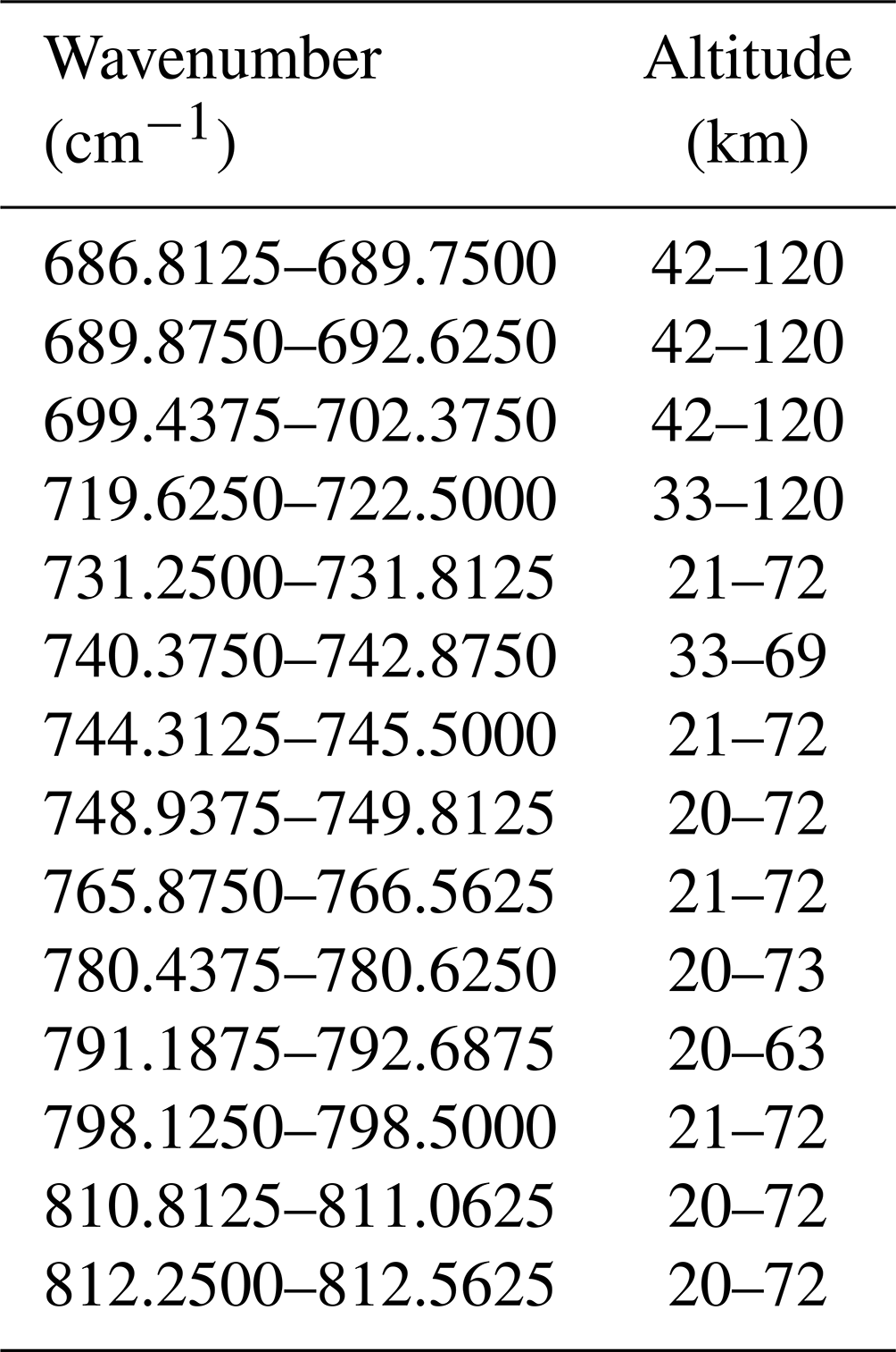
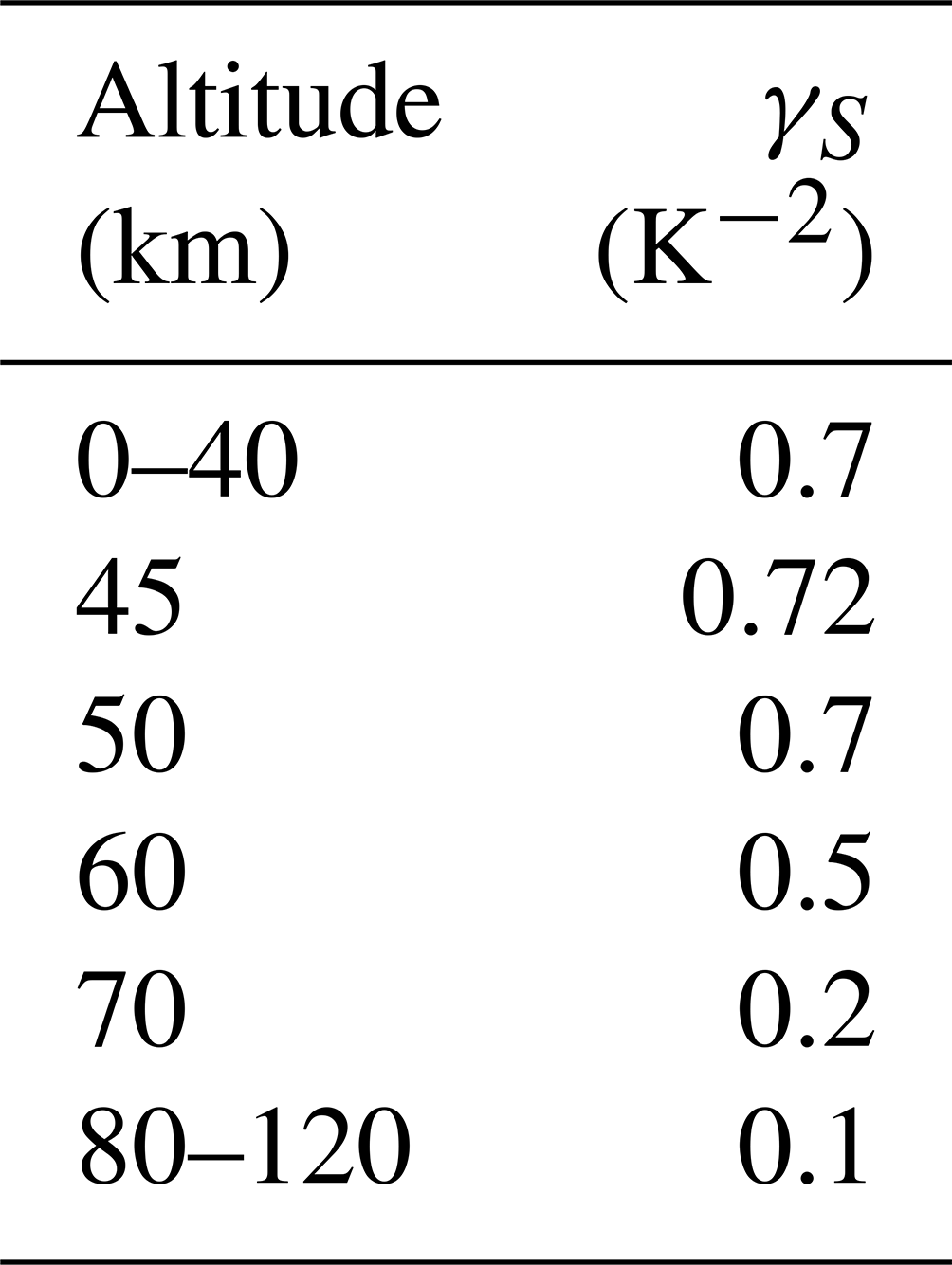
Table 2 Values prescribing the dependence with altitude of the smoothing regularization terms used in version 8 MA, UA and NLC mode temperature retrievals.

Additionally, MA, UA and NLC temperatures are retrieved considering a sophisticated CO₂ non-LTE scheme as described in Funke et al. (2012) (unlike NOM retrievals, which use a parameterized non-LTE climatology). The algorithm jointly fits interfering species (namely ozone and water vapor) and also retrieves the horizontal temperature gradients, the background continuum up to 58 km and an altitude-dependent radiance offset profile. A list of the main aspects of the retrieval baseline follows. Where relevant, we also mention the updates with respect to version V5R_T_m21 retrievals, the previous release of MIPAS IMK–IAA MA, UA and NLC temperatures (García-Comas et al., 2014). For further details on the version 8 retrieval setup, we refer the reader to Sect. 3 of Kiefer et al. (2021).

• MIPAS spectra. The version of the calibrated MIPAS spectra used is the latest supplied by ESA (8.03) (ESA, 2019), which uses a time-dependent correction of the non-linear detector response for the calibration (Birk and Wagner, 2010; Kleinert et al., 2018). Version 5.02/5.06 was used for preceding IMK–IAA version 5 retrievals, which used a preflight characterization. Also, gain calibration has been taken for the corresponding day in version 8.03, whereas it was taken once per week in previous versions (Kleinert et al., 2018).

• Microwindows and spectroscopic data. Table 1 shows the spectral intervals, referred to as microwindows, from where temperature and altitude information of the line of sight is retrieved. This selection of microwindows is almost identical to that used in previous versions of MA, UA and NLC temperature retrievals (García-Comas et al., 2014), except that the width of some microwindows comprising fundamental band lines has been slightly extended at high altitudes to better capture the continuum and the radiance offset. In the search for consistency with MA, UA and NLC temperatures, the version 8 NOM temperature retrievals from reduced-resolution spectra also adopted these microwindows, which was not the case in previous data versions. The spectroscopic database used for most species is the version 2016 HIgh-resolution TRANsmission molecular absorption database (HITRAN 2016; Gordon et al., 2017). We used HITRAN 2008 in version 5. For O₃ and HNO₃, we use a dedicated MIPAS spectroscopic database (Flaud et al., 2003).

• Frequency shift determination. Even though the MIPAS Level 1b data are spectrally calibrated, our retrieval requires adjustments to account for shifts due to the modeling of the instrument line shape. To solve this issue, we derive a frequency shift scale from MIPAS spectra for each scan prior to the temperature retrieval. To avoid noise fluctuations, the spectral shift is retrieved in two iterations. In the first step, the spectral shift is retrieved in a maximum likelihood approach from each individual measurement. The second step uses a maximum a posteriori scheme constrained to the temporal mean and variances of the results from the first iteration. The microwindows used for the frequency shift retrieval are listed in Table 1 of Kiefer et al. (2021). We had to include NO₂ in the forward model because of a significant mesospheric contribution.

• Continuum. Following the findings of Haenel et al. (2015), we now jointly fit the continuum up to 58 km instead of up to 33 km in the version 5 retrievals, which eliminates biases and improves convergence. We use a zero a priori continuum.

• Offset. We derive an altitude-dependent radiance offset for each microwindow to correct for the zero radiance level, constrained to the empirical profile derived by Kleinert et al. (2018). The offset correction is indistinguishable from the continuum above ∼ 30 km, leading to problems with their simultaneous retrieval. We solve this problem by strongly constraining the offset to its a priori profile.

• Temperature regularization. The IMK–IAA MA/UA/NLC temperatures are retrieved from the ground to 120 km at 1 km steps up to 50 km, 2 km steps from 50 to 100 km, 2.5 km steps from 100 to 105 and 5 km steps from 105 to 120 km. Both NOM and MA/UA/NLC retrievals include a first-order-difference Tikhonov regularization that constrains the vertical temperature gradients. Note that, unlike optimal estimation or maximum a posteriori retrievals (Rodgers, 2000), the regularization scheme chosen here does not push the temperatures towards the a priori profiles but only constrains the shape of the temperature profiles. MA/UA/NLC retrievals further use a weak diagonal temperature constraint around 90 km just to prevent unreliable values in the cold polar summer mesopause. Table 2 summarizes the so-called γ values (see Eq. 2 of Kiefer et al., 2021), which govern the altitude variation in the regularization in the MA/UA/NLC retrievals.

• Temperature, pressure and tangent altitude a priori information. As in V8R_T_260 NOM retrievals, temperature a priori information in V8R_T_m61 MA, UA and NLC retrievals is taken from ECMWF ERA-Interim reanalysis fields (Dee et al., 2011) smoothly merged between 43 and 53 km towards bias-corrected Specified Dynamics – Whole Atmosphere Community Climate Model version 4 (SD-WACCM4) (Garcia et al., 2017) at MIPAS geolocations and times. We performed the WACCM temperature bias correction by using the V5R_T_m21 2005-2012 temperature composites (García-Comas et al., 2014). A priori tangent heights come from the line-of-sight engineering information. Pressure is hydrostatically reconstructed above the lowest tangent height, starting with the ECMWF value at that altitude. In V5R_T_m21, the a priori temperature was taken from ECMWF below 65 km and NRLMSISE-00 (Naval Research Laboratory Mass Spectrometer and Incoherent Scatter radar empirical model extended to the Exobase – version 00; Picone et al., 2002) above 65 km.

• Tangent altitude regularization. In contrast to the temperature regularization, for the tangent altitudes a maximum-a-priori-type regularization (Rodgers, 2000) is used, which pushes the retrieved tangent altitudes towards the a priori information. The tangent altitudes are constrained towards ESA's line-of-sight engineering information assuming a 60 m standard deviation in the relative pointing between adjacent tangent altitudes and a 900 m absolute pointing uncertainty, allowing for a vertical shift in the entire limb scan. In the MA/UA/NLC retrievals there is an additional very hard constraint at 105 km towards the engineering values. This update with respect to version 5 retrievals is motivated by the results of Jurado-Navarro et al. (2016). They retrieved very small deviations of the tangent altitudes in the lower thermosphere from the engineering tangent altitudes using MIPAS 4.3 µm measurements.

• Trace gas distributions. The CO₂ abundances used to simulate the spectra are extracted from SD-WACCM4 climatology, while H₂O and O₃ abundance profiles are taken from MIPAS version 5 retrievals (García-Comas et al., 2016b; López-Puertas et al., 2018).

Regarding atomic oxygen, we have revised the calculation scheme in version 8 MA/UA/NLC temperature retrievals in order to use more realistic abundances than those in the version 5 retrievals, where O came from NRLMSISE-00. We recall that atomic oxygen affects the temperature retrievals mainly through the non-LTE CO₂ vibrational populations. We now derive O using the following approach. The O_x and H used to determine O are taken from bias-corrected WACCM4 at MIPAS geolocations. This bias correction for WACCM4 O_x is estimated using the MIPAS O₃ daytime climatology (versions V5_O3_522; López-Puertas et al., 2018) under consideration of photochemical equilibrium. In addition, since the WACCM bias is estimated from MIPAS daytime measurements, a tidal correction is applied to account for day–night differences as described in Sect. 2.2.4 of López-Puertas et al. (2023). The bias correction for H, required for nighttime measurements, is obtained from the ratio of MIPAS version 5 daytime and nighttime O₃ climatologies as also described by López-Puertas et al. (2023). Finally, O is calculated from the bias-corrected O_x and H by means of photochemical box modeling using ozone photoabsorption coefficients based on the Tropospheric Ultraviolet and Visible (TUV) radiation model version 5.2 driven by the Climate Model Intercomparison Project round 6 (CMIP6) solar irradiance variations. This approach is made to preserve the transient variability as provided by WACCM4 while retaining the climatological atomic oxygen as derived from MIPAS measurements in the previous version. The atomic oxygen derived in this way is reliable below 97 km. Above 97 km, we use the atomic oxygen from SD-WACCM4 simulations at MIPAS geolocations.

• Temperature horizontal inhomogeneity retrieval. It was shown by von Clarmann et al. (2009a) that MIPAS limb radiances originate up to ± 400 km around the tangent point. We therefore derive horizontal temperature gradients as described in Kiefer et al. (2021). We prescribe a full 3D temperature field constructed from ECMWF ERA-Interim temperatures below 60 km and NRLMSISE-00 temperatures above, and we retrieve the linear corrections to this field. Version 5 retrievals only allowed for a linear correction of horizontal temperature gradients from ECMWF-40.

• Forward model numerical settings. The spectral grid for the monochromatic radiance calculations is $\mathrm{5}\times {\mathrm{10}}^{-\mathrm{4}}$ cm⁻¹. The computational accuracy of the absorption coefficient calculations in the forward model is now improved with respect to version 5. We use five pencil beams to numerically integrate the signal in the vertical direction over the field of view.

• Non-LTE treatment. The most salient difference between the V8R_T_261 NOM mode temperature retrievals described in Kiefer et al. (2021) and the V8R_T_m61 MA, UA and NLC mode retrievals described here is that, instead of using climatological CO₂ vibrational-level populations, we explicitly calculate the CO₂ vibrational-level populations for the atmospheric conditions of each scan. This is essential for the accurate retrieval of temperatures above 70 km. The non-LTE population calculations are performed at each iteration of the retrieval loop with the Generic RAdiative traNsfer AnD non-LTE population Algorithm (GRANADA) and the non-LTE setup described in Funke et al. (2012). The non-LTE collisional rates affecting 4.3 µm CO₂ levels have been slightly changed with respect to those in Funke et al. (2012) using the values derived from Jurado-Navarro (2015), but this has a negligible impact on the 15 µm levels. We also correct the non-LTE populations along the line of sight according to the simultaneously retrieved horizontal temperature gradient, which is particularly relevant when the line of sight crosses the poles during the solstices. The line-by-line Karlsruhe Optimized and Precise Radiative transfer Algorithm (KOPRA) forward model (Stiller et al., 2002), one of the processor modules which is internally interfaced with the GRANADA algorithm, then simulates the 15 µm CO₂ emission using these non-LTE populations. The non-LTE scheme and collisional rates in these V8R_T_m61 retrievals are the same as in the previous V5R_T_m61 retrievals.

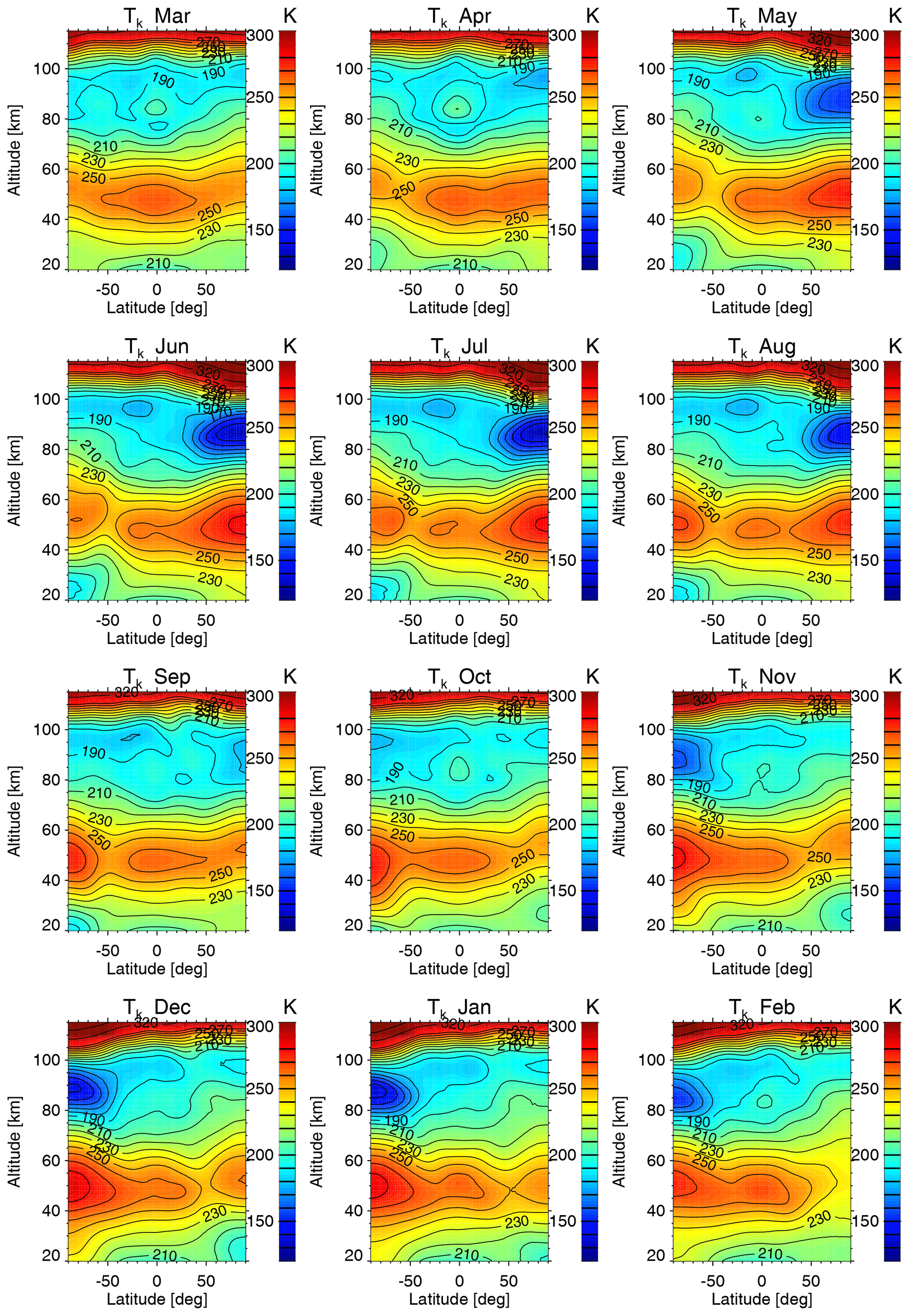
Figure 1 MIPAS version 8 MA/UA composite monthly zonal mean temperature. Contour levels are indicated in the color bars (every 10 K up to 280 K and then every 40 K).

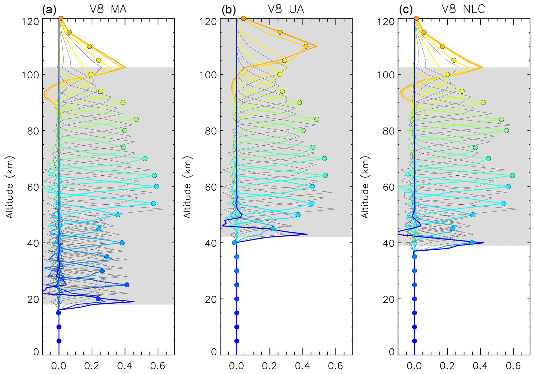
Figure 2 Example averaging kernel rows of the retrieved temperatures from MA (a), UA (b) and NLC (c) version 8 measurements. Rows for retrievals from 5 to 120 km every 5 km are shown in color, and the corresponding diagonal element values are shown with circles. Shaded areas indicate the altitude range of the measurements. The examples belong to measurements around latitudes of 30^∘ N/S.

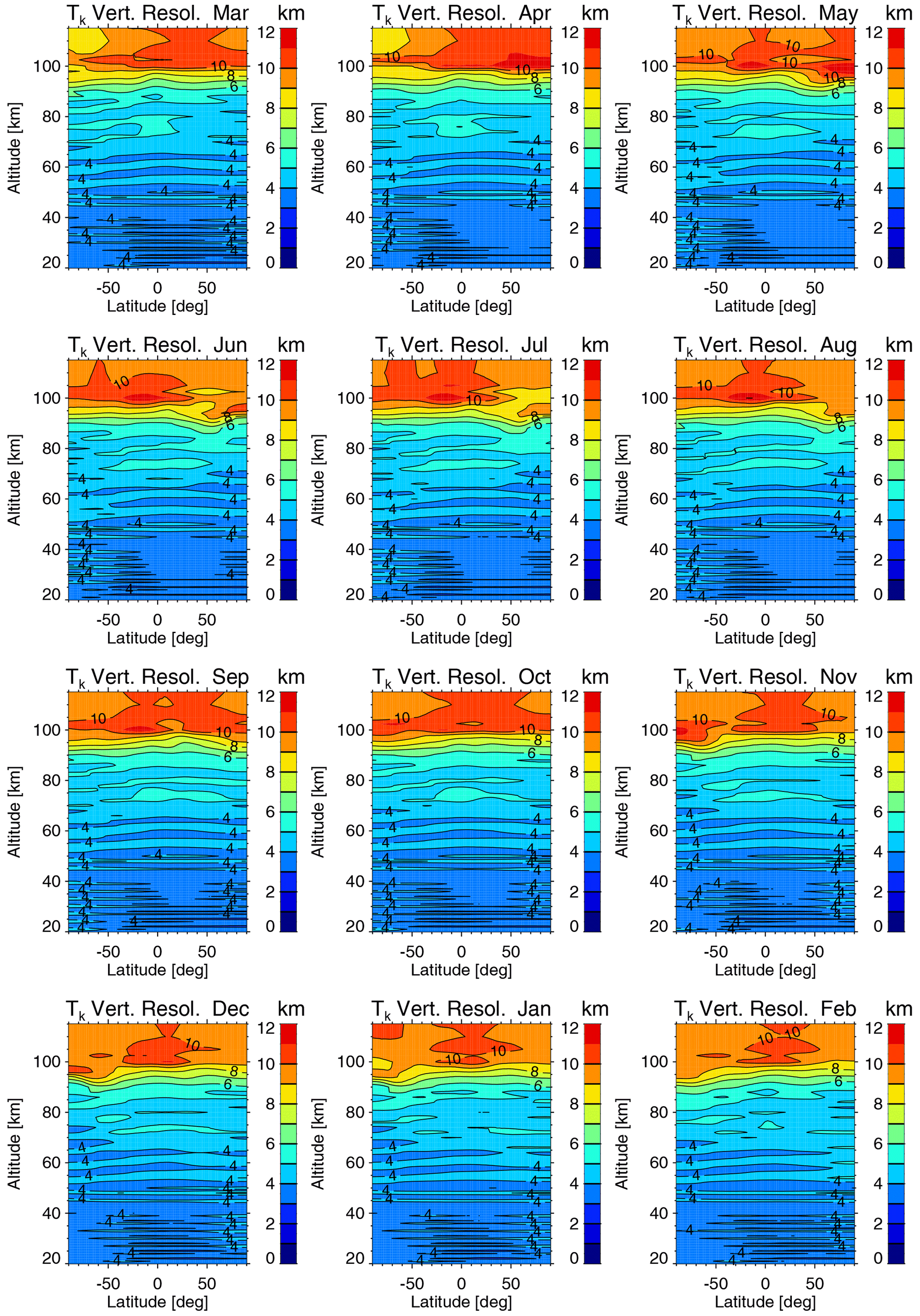
Figure 3 MIPAS version 8 MA/UA composite monthly temperature vertical resolution. Contour levels are indicated in the color bars (every 1 km from up to ± 10 km and then 12 km.

Figure 1 shows the 2007–2012 composite of version 8 MA/UA zonal mean temperatures for each calendar month. They correspond to the zonal means of all available MIPAS measurements at geolocations within ± 5^∘ in latitude to each grid point. We do not include in this figure NLC and 2005–2006 MA/UA temperatures because they do not provide a regular temporal coverage along the natural year. We focus here more on the MIPAS temperatures in the MLT region, since the stratosphere was well covered by the NOM measurements, and Kiefer et al. (2021) have already discussed the stratospheric temperatures. We present temperatures up to 115 km. Several features related to well-known mechanisms are evident in Fig. 1:

• Lower-thermospheric temperatures are highest during the polar summer (300 K at 105 km and 370 K at 115 km) and lowest during the polar winter and the equatorial equinoxes (210 K at 105 km and 330 K at 115 km) due to the corresponding variation in total insolation.

• The meridional circulation, controlled by gravity wave filtering, causes the positive summer-to-winter latitudinal gradients of mesopause temperature and mesopause altitude (Garcia and Solomon, 1985) and leads to MIPAS mesopauses at 130–140 K and 86–88 km in polar summer and at 180 K and 98 km in polar winter.

• The mesospheric semi-annual oscillation (SAO), caused by the filtering of gravity waves by the stratospheric wind SAO (Dunkerton, 1982), is responsible for the local maximum at 85 km at low latitudes that occurs during the equinox months and leads to peak temperatures of 220 K in April (seen in the Fig. 1 as a yellowish isolated blob).

• The typical polar summer transition from maximum ozone heating in the low mesosphere to maximum cooling from upwelling in the high mesosphere results in the largest mesospheric temperature vertical gradients, which maximize in June and July in the Northern Hemisphere (NH) and in December and January in the Southern Hemisphere (SH).

• The average mesospheric vertical gradients of heating due to downwelling during the polar night winter months result in minimum mesospheric temperature vertical gradients in February in the NH and May–June in the SH. Note that this average behavior in the NH is influenced by the occurrence of elevated stratopause events, where the temperature vertical gradients become positive (Manney et al., 2005).

• The vertical deflection of the polar winter vortex to lower latitudes (Fleming et al., 1990) and the associated diabatic descent from gravity-wave-driven circulation (Hitchman et al., 1989) result in the wrinkled mid- to upper-mesospheric temperature contours from May to August in the SH and from October to March in the NH. These even lead to a distinct warmer mesopause centered around 50–60^∘ N in December and January in MIPAS data.

2.1 Retrieval performance

Figure 2 shows typical averaging kernel rows of the retrieved MA, UA and NLC version 8 temperatures. Our recommendation for the data users is to discard data points at altitudes where the corresponding averaging kernel diagonal element is less than 0.03 because they lack significant measurement information. There is temperature information from 18 to 110 km for MA measurements (starting at 39 km for NLC measurements) and from 42 to 115 km for UA measurements. The shifts between the peaks of the averaging kernels and the tangent heights observed at the highest altitudes (above 102 km tangent heights in MA and NLC and above 110 km tangent heights in UA) emphasize the paramount importance of taking these averaging kernels into account when interpreting the data or when comparing temperatures with results from climate models or other temperature measurements. The averaging kernel matrix for each individual temperature profile is available with the data.

For each individual MIPAS temperature profile in our data, we provide the corresponding values of the vertical resolution, estimated as the full width at half maximum of the corresponding averaging kernel. Figure 3 shows the 2007–2012 composite of the vertical resolution of the MA/UA temperature profiles. It is about 3 km at altitudes below 50 km, 3–5 km at 50–70 km, 4–6 km at 70–90 km, 6–10 km at 90–100 km and 8–11 km at 100–115 km. The oscillating behavior depicted arises because the vertical resolution is better at retrieval altitudes closer to the tangent altitudes (see Fig. 2), despite the larger error introduced by measurement noise. The vertical resolution of temperature shows no significant dependence on latitude or season, although it is slightly coarser at 90–100 km in the polar summer.

3 Error budget

Estimating the error budget for each individual MIPAS profile is computationally expensive. Rather than performing calculations for each profile, we have selected sets of uniformly distributed individual measurement profiles representative of typical atmospheric conditions, for which we estimated the temperature errors. We selected sets of about 30 geolocations for 5 latitude boxes (northern and southern poles, namely 65–90^∘ N and S; northern and southern mid-latitudes, namely 40–60^∘ N and S; and tropical, namely 20^∘ S–20^∘ N) in the four seasons and during the day and night, resulting in 34 different atmospheric scenarios. Each component of the temperature error for each of these atmospheric conditions is then the mean of the corresponding component calculated for the individual geolocations within the set.

Table 3 summarizes the sources of temperature errors considered in our calculations and the associated uncertainties. All reported uncertainties are 1 σ throughout. The assumed uncertainties are the same as those used by Kiefer et al. (2021) with the exception of the uncertainties related to the gain calibration, radiance offset and the non-LTE model. Except for the later, the assumptions made for their estimation are described in von Clarmann et al. (2022). We shortly justify the assumed uncertainties here.

Kleinert et al. (2018)Hase (2003)Kleinert et al. (2018)Kiefer et al. (2021)López-Puertas et al. (2017)López-Puertas et al. (2017)López-Puertas et al. (2017)López-Puertas et al. (2018)García-Comas et al. (2012)García-Comas et al. (2012)García-Comas et al. (2012)

Table 3 Temperature error sources and corresponding uncertainties considered in this work. The “Char.” column indicates if the error source chiefly causes a systematic (sys) or a random (ran) error. Error sources in each of the three sections of the table are listed following their decreasing relative contribution to temperature errors in decreasing order.

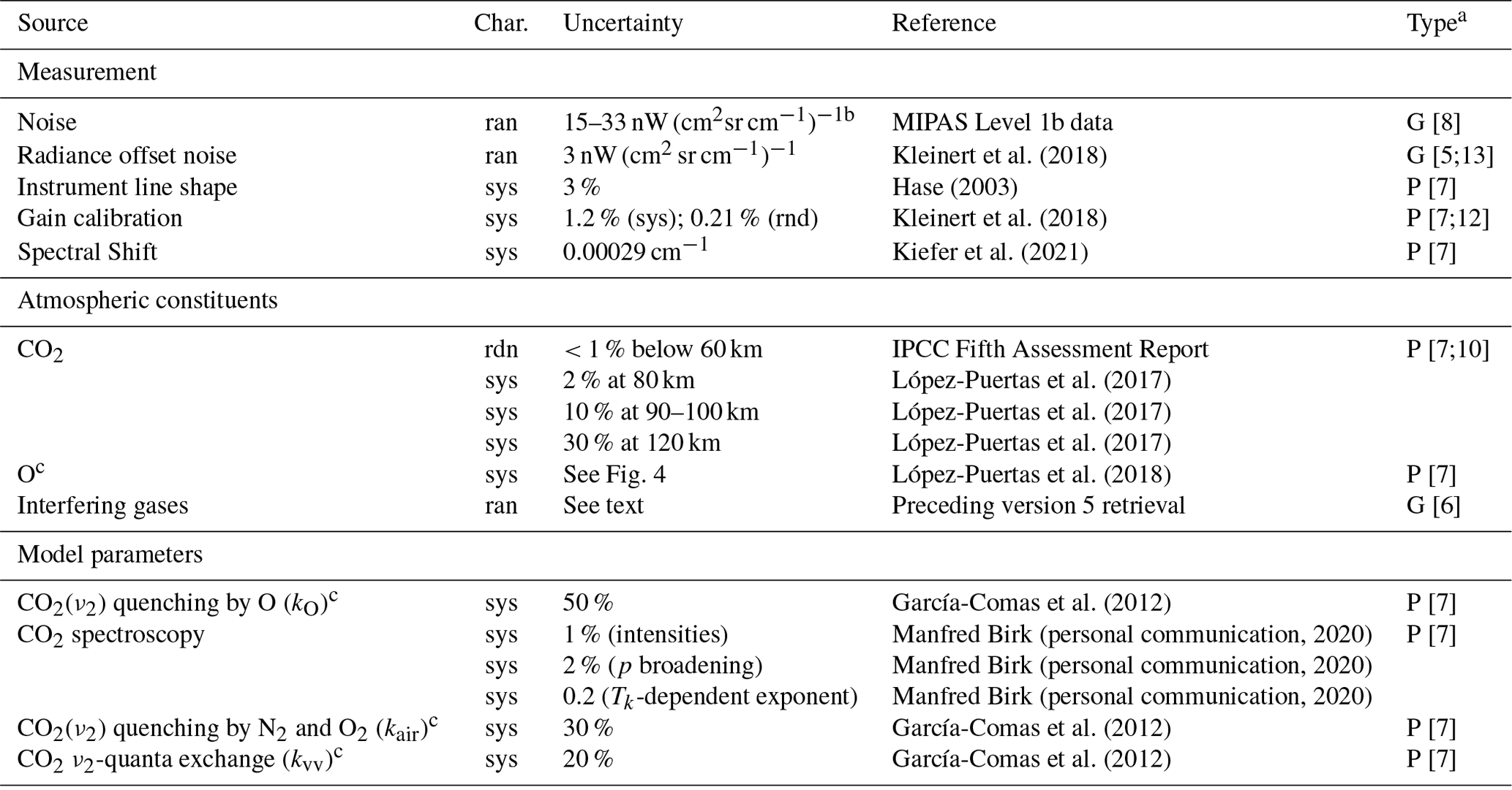
^a Error calculation propagation method: (G) generalized Gaussian error propagation in a matrix formalism, (P) via perturbation spectra. The numbers in brackets refer to the equation in von Clarmann et al. (2022), where the respective input uncertainty is applied. ^b After apodization. ^c Non-LTE error sources.

• Measurement noise. The temperature noise error accounts for the propagation of the measurement noise through the retrieval for single scans, calculated using the Level 1b wavelength-dependent noise-equivalent spectral radiance (15–33 nW (cm² cm⁻¹ sr)⁻¹ in the spectral region within MIPAS Band A used for temperature retrievals).

• Radiance offset noise. Although we have retrieved radiance offset together with the temperature, there is still a remaining random uncertainty due to the wavelength dependence of the deep-space measurements used for the Level 1b radiance offset calibration. We estimated the radiance offset uncertainty following the description in von Clarmann et al. (2022), which results in 3 nW (cm² cm⁻¹ sr)⁻¹ for MIPAS Band A working at reduced resolution.

• Instrument line shape (ILS) uncertainties. We followed the recommendations of Hase (2003) regarding uncertainties in the MIPAS instrument line shape (3 %), characterized by the corresponding estimates of modulation loss through self-apodization.

• Gain calibration uncertainties. We estimated temperature errors separately for the systematic and for the random components of the gain calibration uncertainty. We assumed a systematic uncertainty of 1.1 % (1 σ) for the gain calibration, rescaled from the maximum scaling difference of 1.5 % (2 σ) due to the calibration blackbody and the correction of the detector non-linearity (Kleinert et al., 2018). We have also considered a 0.2 % gain calibration noise.

• Shift uncertainties. We estimated the uncertainty in the frequency shift to be 0.00029 cm⁻¹ (see Kiefer et al., 2021), based on the deviation of the retrieved values from their linear fit along the wavelength.

• CO₂ abundance uncertainty. We assumed CO₂ volume mixing ratio uncertainties of 0.2 % below 30 km, 0.5 % at 40 km, 1 % at 60–80 km, 10 % at 90–100 km and 20 % at 110 km. Below 60 km, these were based on uncertainties according to the Intergovernmental Panel on Climate Change (IPCC) Fifth Assessment Report and also took into account CO₂ seasonal variability uncertainties. Above 60 km, we used the uncertainties estimated from previous comparisons of WACCM CO₂ at MIPAS geolocations with the Atmospheric Chemistry Experiment Fourier transform spectrometer (ACE-FTS) and SABER observations (López-Puertas et al., 2017). CO₂ uncertainties are positively correlated over small spatial or temporal scales and should be considered to be sources of systematic errors for localized comparisons with other instruments. In general, CO₂ uncertainties should be considered to be systematic errors above 60 km.

• CO₂ spectroscopy uncertainty. Temperatures are retrieved from CO₂ emission lines using spectroscopic information from the HITRAN 2016 database. Uncertainties in the spectroscopy of the CO₂ lines are considered following recommendations by Manfred Birk (personal communication, 2020), namely a 1 % uncertainty in the intensity, a 2 % uncertainty in the pressure-broadening coefficient and a 0.2 absolute uncertainty in the exponent for temperature dependence.

• Interfering gas uncertainty. For gases derived in preceding MIPAS version 5 retrievals, we have used the noise covariance information obtained from those retrievals. For interfering gases not previously retrieved from MIPAS measurements, we relied on our initial guess database (Kiefer et al., 2002, and updates thereof). In the later case, accurate uncertainty information for the abundances is often unavailable, and we have assumed a 100 % uncertainty. The contribution of these uncertainties to the temperature error is significantly smaller than the total error, rendering a more detailed assessment unnecessary.

• Non-LTE modeling uncertainties. The main source of error above the mid-mesosphere arises from uncertainties in the non-LTE modeling, which are mainly due to three collisional rates and the atomic oxygen abundance. Based on the considerations of García-Comas et al. (2012), we have assumed uncertainties of ± 20 % for the rate of vibrational exchange of ν₂ quanta between CO₂ molecules, ± 30 % for the quenching of the CO₂(ν₂) states through collisions with N₂ and O₂, and ± 50 % for the quenching of the CO₂(ν₂) states by atomic oxygen.

The atomic oxygen below 95 km used in our temperature retrievals comes on average from MIPAS version 5 daytime retrievals (we note that it is scaled for nighttime). Following López-Puertas et al. (2018) (see their Eqs. 5 and 6), we have estimated the atomic oxygen uncertainty by assuming their ozone abundance errors, a 10 % uncertainty in the three-body reaction rate of O₃ formation and a 5 % error in the ozone photodissociation. Above 95 km, we have estimated the uncertainty in the atomic oxygen used in our retrievals coming from WACCM from comparisons with version 2.0 Naval Research Laboratory Mass Spectrometer and Incoherent Scatter radar empirical model (NRLMSIS 2.0) atomic oxygen (Emmert et al., 2021). Estimates were made for five different latitude boxes, for the four seasons and for day and night. On average, the uncertainties range from 25–30 % at 85 km to 5 % at 120 km (Fig. 4). Below this altitude, the nighttime uncertainties are significantly larger, reaching 120 % at 70 km.

Following the recommendations of TUNER (Towards Unified Error Reporting; von Clarmann et al., 2020), we discuss systematic and random errors separately. This is useful because, for example, while the characterization of systematic errors is essential for the identification of measurement biases, they require less attention when evaluating atmospheric waves, atmospheric trends or instrumental drifts. The methodology used in this work to estimate the contribution of the various error components to the temperature errors is described in great detail in von Clarmann et al. (2022). We assume linear error propagation. Depending on the characteristics of each error source and the available information on its uncertainty, we chose between two different methods of error propagation: Gaussian or perturbation (see last column in Table 3). We applied Gaussian error propagation when the covariance matrix in the measurement domain was known (von Clarmann et al., 2022, Eqs. 5 and 6 therein), i.e., for measurement noise, noise impact on the radiance offset calibration measurement and noise-induced interfering gas uncertainties. We applied perturbation error propagation (von Clarmann et al., 2022, Eq. 7 therein) when using the Gaussian approach was not possible due to unavailability of covariance information or when it was not appropriate, i.e., for ILS, gain calibration, spectral shift, CO₂ abundance, CO₂ spectroscopy and non-LTE uncertainties. There were error sources for which no specific values of their random uncertainty could be prescribed (for instance, CO₂ abundance, CO₂ spectroscopy, non-LTE and ILS). Since temperature errors triggered by a systematic parameter uncertainty also exhibit a random component due to atmospheric variability, we also conducted statistical analyses on the responses to perturbations across the ensemble of temperature profiles, each ensemble representing a distinct atmospheric scenario. We took the dispersion within these responses as an estimate of the associated random component of the temperature error for those cases.

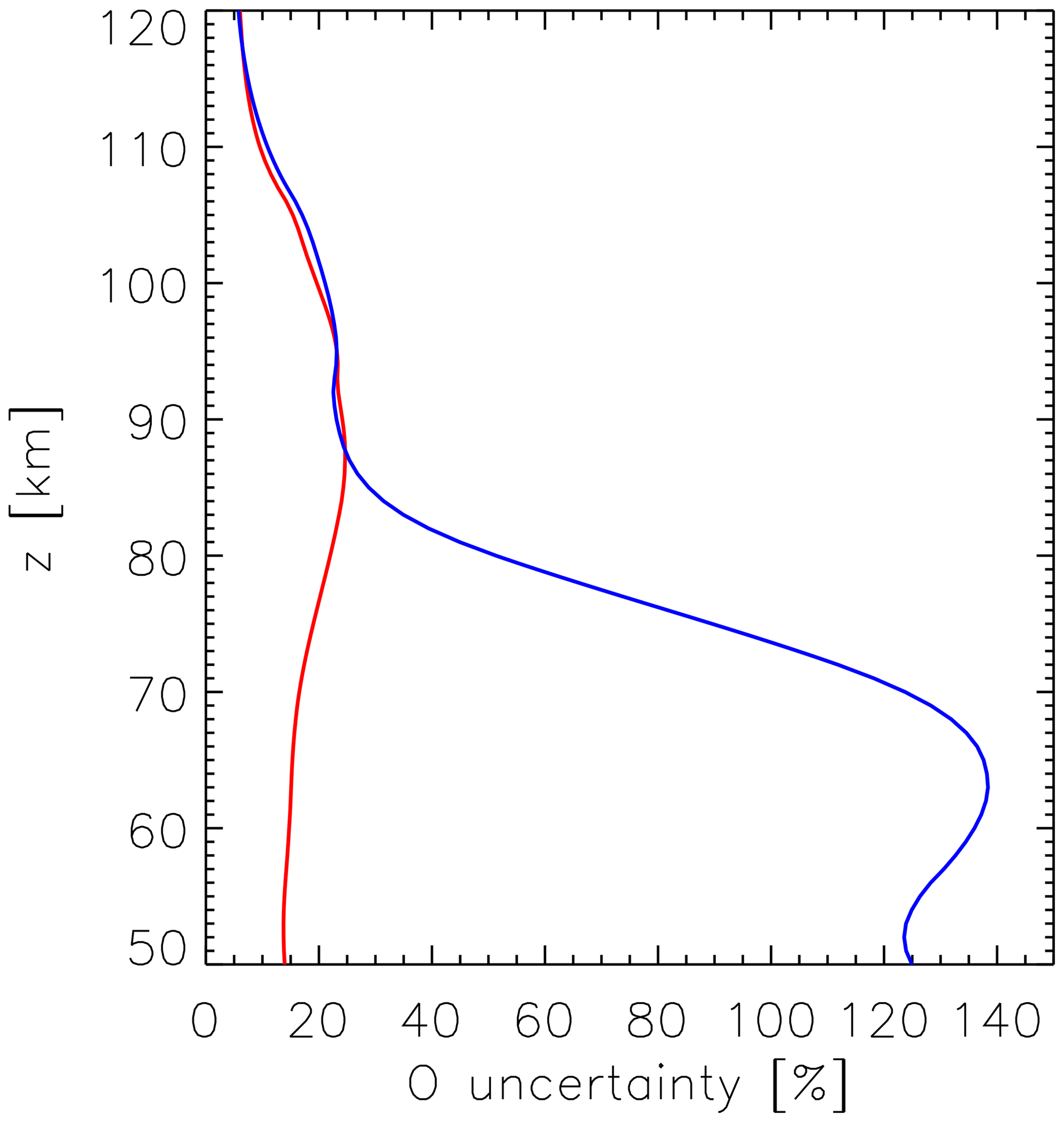
Figure 4 Estimated daytime (red) and nighttime (blue) uncertainties in atomic oxygen abundance averaged across all seasons and latitudes.

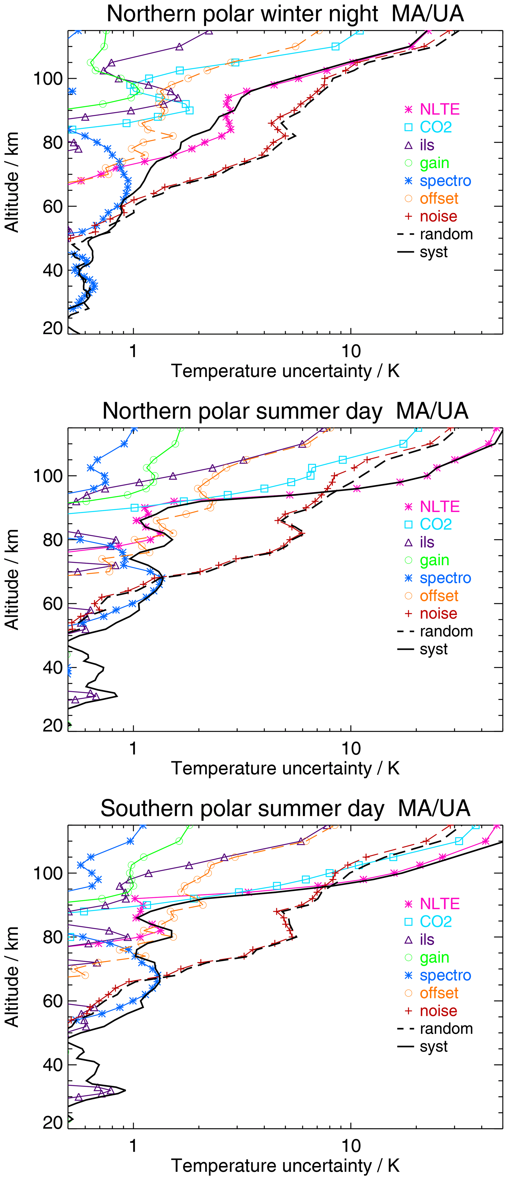
Figure 5 MIPAS version 8 MA/UA temperature uncertainties for a few representative polar atmospheric scenarios. Errors that are chiefly random are indicated with dashed lines, and errors that are chiefly systematic are indicated with solid lines. The corresponding error values are listed in Table A1 of the Appendix.

Figure 6 As Fig. 5 but for representative mid-latitude atmospheric scenarios. The corresponding error values are listed in Tables A2 and A3.

Figure 7 As Fig. 5 but for representative tropical atmospheric scenarios. The corresponding error values are listed in Table A4 of the Appendix.

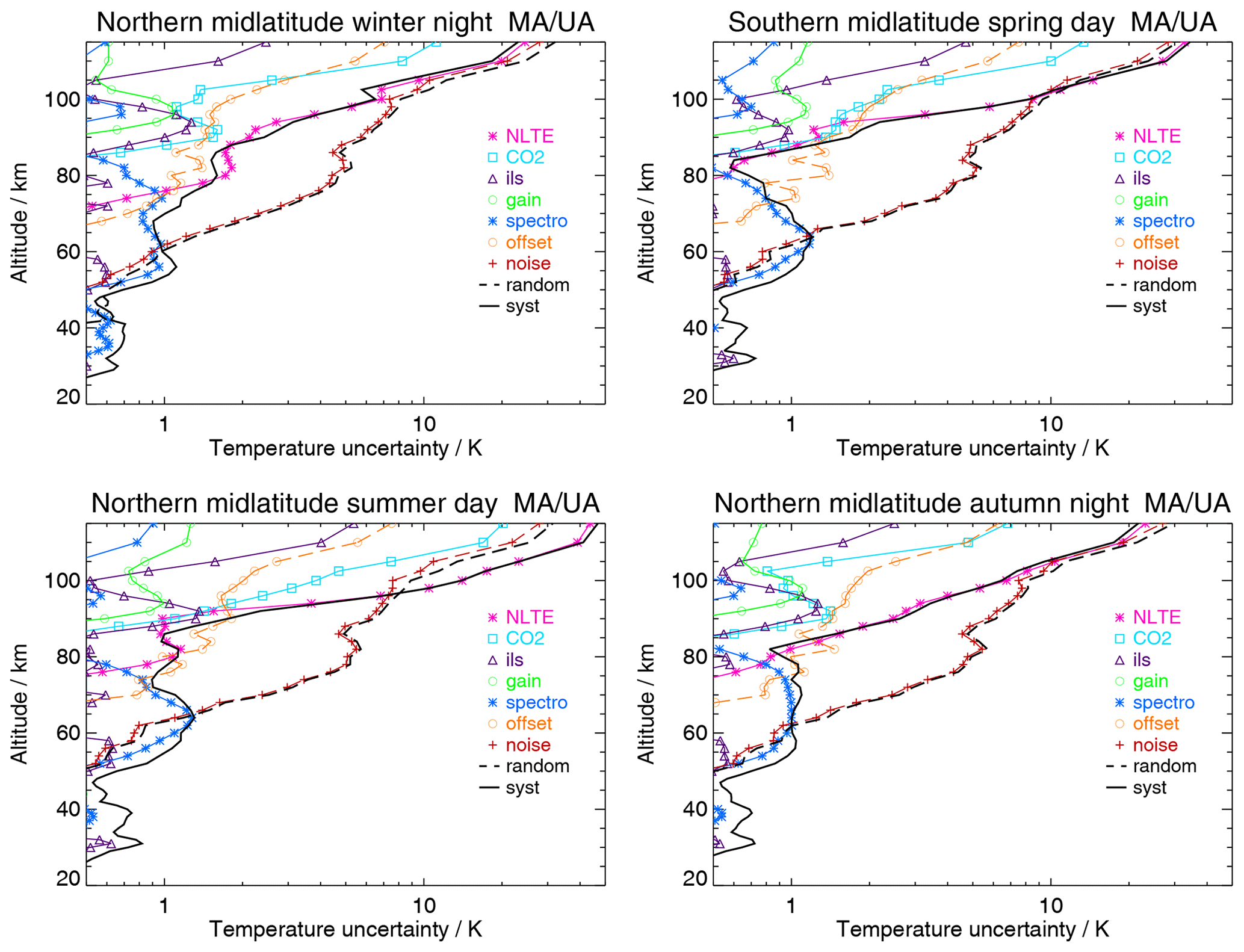
Figures 5, 6 and 7 and the corresponding Tables A1–A4 in the Appendix provide the overall random and systematic MIPAS version 8 MA/UA temperature errors for representative polar (65–90^∘ N and S), mid-latitude (40–60^∘ N and S) and tropical (20^∘ S–20^∘ N) atmospheric scenarios, respectively, for selected seasons. The figures also show the contributions of the different error sources to the total error. Chiefly random errors are indicated with dashed lines, and chiefly systematic errors are indicated with solid lines. This is only a selection of all the atmospheric scenarios we have considered. The Supplement of this paper contains a collection of the MIPAS MA/UA temperature error budgets for the 34 representative atmospheric conditions for day and night of spring, summer, autumn and winter conditions at polar latitudes, at mid-latitudes and in the tropics (see Table S1 in the Supplement).

The MA/UA MIPAS temperature error budget behaves similarly to that for NOM at altitudes where MA/UA and NOM measurements overlap (below 68 km; see Kiefer et al., 2021). We focus our discussion here on the mesosphere and lower thermosphere. For the sake of completeness, we show the errors in the full altitude range covered by the MA/UA measurements.

3.1 Random errors

By far the largest contributor to the MIPAS random temperature error, which accounts for the standard deviation of the temperature, is the measurement noise. The noise error is less than 1 K at altitudes below 60 km, 1–3 K at 60–70 km, 3–5 K at 70–90 km, 6–8 K at 90–100 km, 8–12 K at 100–105 km and 12–20 K at 105–115 km (see Figs. 5–7 and the corresponding Tables A1–A4 in the Appendix).

The noise error does not exhibit a significant dependence with latitude or season, although it increases slightly around the polar summer mesopause (due to the lower temperatures there).

Less important than the measurement noise but still non-negligible contributors to random temperature errors in the mesosphere and above are the following. The radiance offset noise typically results in random errors smaller than 0.5 K below 70 km, 1 K at 80 km, 2 K at 100 km and 5–7 K at 110–115 km. The CO₂ mixing ratios typically yield random errors smaller than 0.5 K below 90 km, 1–3 K at 105 km and 3–7 K at 115 km. The ILS uncertainties result in temperature errors less than 0.5 K below 80 km, 0.5–1 K at 80–105 km and 2 K at 115 km. Note that these random components are not shown individually in the figures.

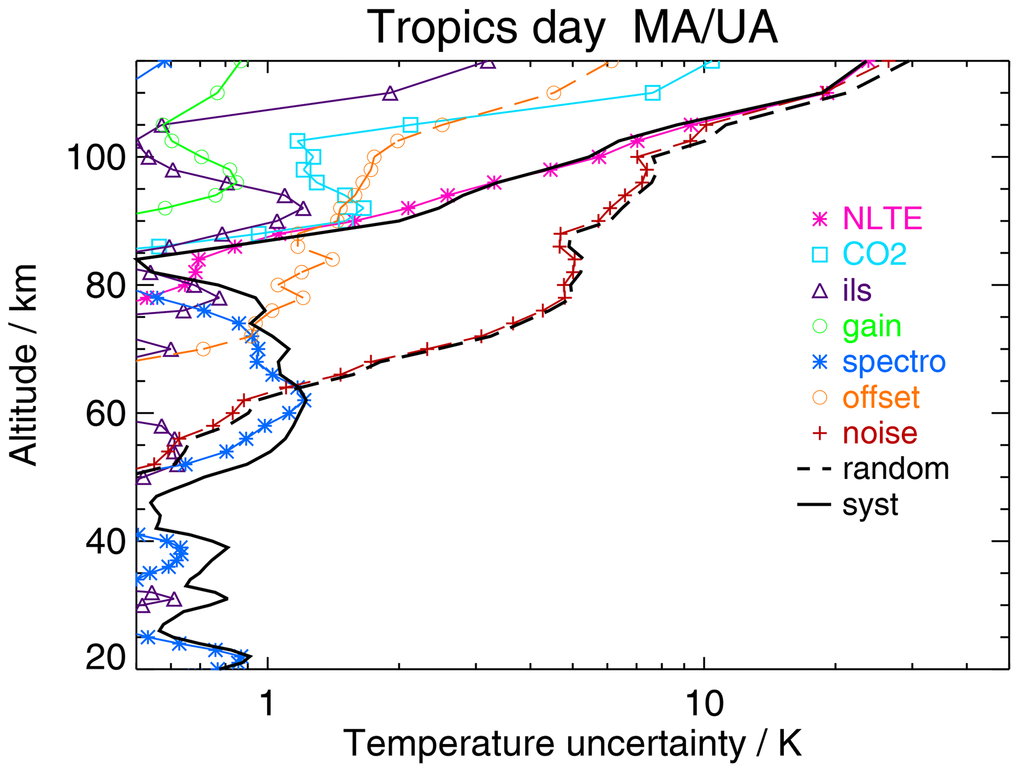
Random temperature errors due to non-LTE model uncertainties are shown with dashed lines in Fig. 8. They are typically less than 1 K below 95 km (1.5 K for polar winter), 5 K at 105 km and 10 K at 115 km. The uncertainty in the CO₂–O quenching rate (k_O) is primarily responsible for these random errors, followed by uncertainties in the atomic oxygen abundance and, only under polar conditions around 80 km, the CO₂ quenching by N₂ and O₂ (k_air). According to our calculations, all other potential sources produce random temperature errors smaller than 0.5 K at all altitudes.

Figure 8 MIPAS version 8 MA/UA systematic (solid line) and random (dashed lines) temperature errors due to non-LTE model uncertainties, i.e., uncertainties in atomic oxygen abundance (blue), rates of CO₂(ν₂) quenching by O (green) and by N₂ and O₂ (orange), and rate of ν₂ exchange between CO₂ molecules (violet).

With respect to typical random errors in the tangent altitude correction, mainly arising from the instrumental noise, we found average values of 50–60 m up to 60 km, decreasing linearly to values smaller than 20 m above 95 km (we recall here that we applied a very hard retrieval constraint towards ESA engineering tangent altitudes at 105 km).

3.2 Systematic errors

Figures 5–7 and the corresponding Tables A1–A4 in the Appendix also show the MIPAS systematic temperature errors, accounting for temperature biases. The main sources of systematic errors above the stratopause are the uncertainties in the CO₂ spectroscopic data (which govern the errors in the lower mesosphere, below 75 km), the non-LTE model parameters (which generally dominate above 75–80 km), the CO₂ abundance, the instrument line shape and the gain calibration.

The spectroscopic information uncertainties typically lead to systematic errors smaller than 0.7 K below 55 km and around 1 K at 60–70 km. They are less than 0.5 K above 80 km, although they increase slightly in the lower thermosphere during the summer.

The overall non-LTE systematic temperature errors, together with the contributions of each non-LTE model parameter uncertainty, are shown as solid lines in Fig. 8. They are highly dependent on the atmospheric conditions. Overall, non-LTE systematic errors are smaller than 0.5 K typically below 75–80 km and below 65–70 km for the polar and mid-latitude winters. The lower altitude for the latter is due to the contribution of the k_air uncertainty. These errors generally increase to 1 K at 80–90 km in the mid-latitude and polar summers, due to the contribution of k_air and k_vv uncertainties, and to 2 K in the polar winter, mainly due to the contribution of the k_O uncertainty.

At 95 km and above, the uncertainty in k_O clearly dominates the non-LTE systematic error and thus the total systematic error (Figs. 5–7). Non-LTE errors and, thus, total systematic error generally reach 3 K at 95 km, 6–8 K at 100 km, 10–20 K at 105 km and 20–30 K at 115 km. For the mid-latitude and polar summers, they are somewhat larger (4–5 K at 95 km, 10–15 K at 100 km, 20–30 K at 105 km and 40–50 K at 115 km), due to the enhanced non-LTE effect for the steep temperature gradient and large temperatures for these conditions. The error due to the atomic oxygen abundance uncertainty displays contributions larger than 1 K above 100 km (95 km in the polar summer) but is significantly smaller than that due to k_O. In fact, we estimate that the second-largest contributor to the systematic temperature error above 90–95 km, after k_O but before the atomic oxygen abundance uncertainty, is the uncertainty in the CO₂ abundance. It has little effect (<1 K) at lower altitudes but yields typical errors of 1–2 K at 95–105 km and 7–10 K at 110–115 km and errors of 2–7 K at 95–105 km and around 20 K at 115 km in the mid-latitude and polar summers.

The ILS uncertainty has some effect at mesospheric altitudes but is generally smaller than 0.5–0.7 K below 80 km, i.e., smaller than that coming from the CO₂ spectroscopy. It is comparable to that of the CO₂ or the k_O uncertainties at 85–90 km but always becomes smaller than both above 95 km.

The contribution of the radiance gain uncertainty is even smaller than that of the ILS. Other potential sources of systematic errors we considered, such as the spectral shift or interference by N₂O₅, cause errors smaller than 0.5 K at all altitudes. They are listed in Table 3, but their effects are not visible in the figures.

As for the typical systematic errors in the tangent altitude correction, mainly arising from the CO₂ spectroscopic uncertainties, they are on average 250 m at 20 km and 200 m from 40 to 60 km, decreasing linearly to 100 m at 80 km and smaller than 50 m above 90 km.

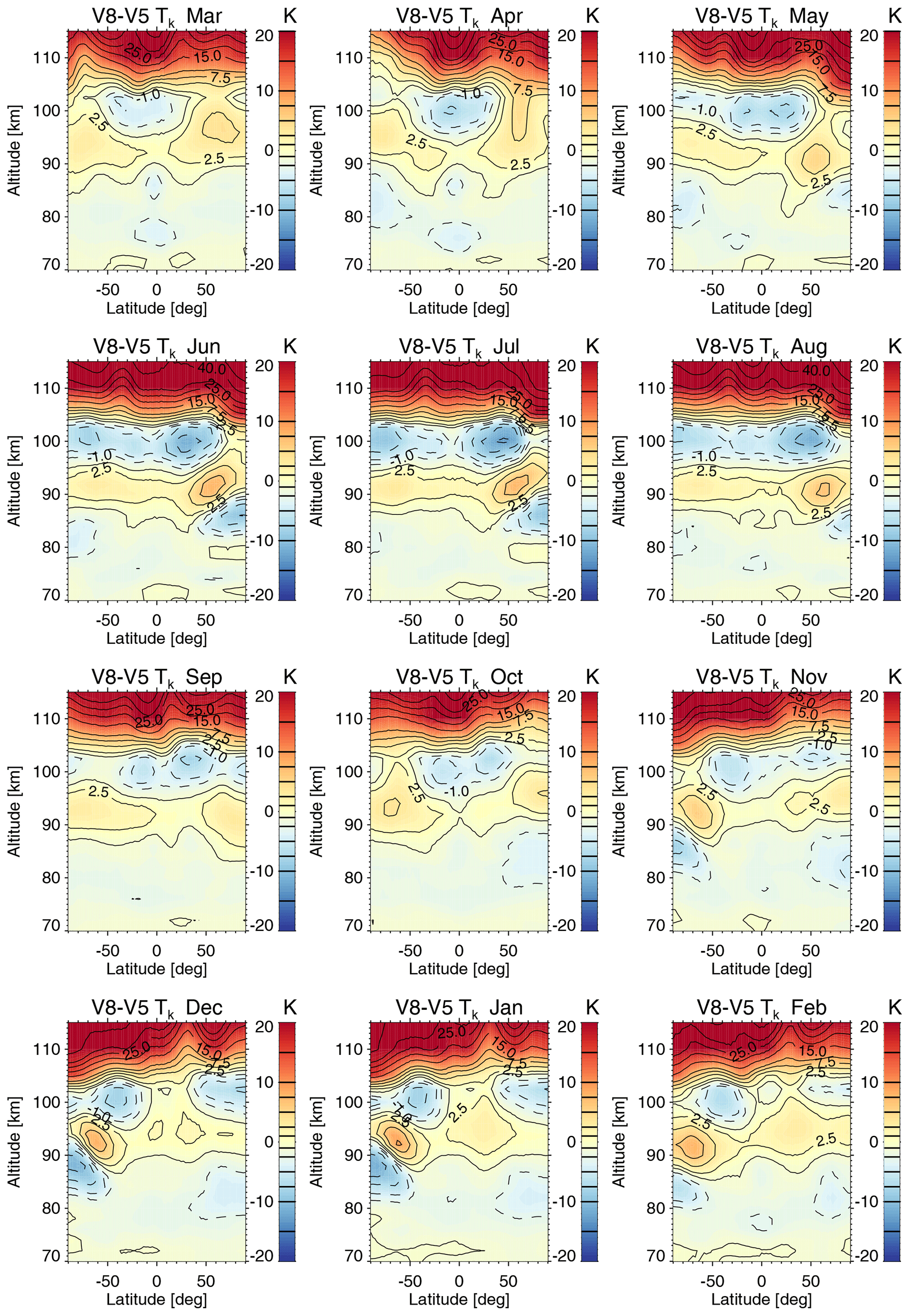
Figure 9 MIPAS version 8 and version 5 MA/UA zonal mean temperature differences. Contour levels are indicated in the color bars (± 1, ± 2.5, ± 5, ± 7.5 and ± 10 K and then every ± 5 K above that value).

4 Temperature differences between the current version 8 and the previous version 5 MA/UA data versions

The improvements in version 8 of MA/UA/NLC temperature retrievals over the previous version 5 are listed in Sect. 2. The resulting differences between the two versions are dominated by the changes in the atomic oxygen and carbon dioxide abundances and in the a priori temperature gradients. Figure 9 shows the differences in the retrieved temperatures produced by these upgrades. We have limited the figure to altitudes above 70 km because the differences below are less than 0.5 K.

As we show in Fig. 9, the change in this new temperature dataset with respect to the previous version at tropical and mid-latitudes has a vertically oscillating structure up to about 105 km, with alternating positive and negative differences, somewhat more pronounced during March, April and May. The differences are negative and smaller than 1 K (in absolute value) below 85 km, positive and smaller than 3 K between 85 and 95 km, and negative and also smaller than 3 K (in absolute value) between 95 and 105 km. This is a manifestation of the better representation of the tides in the MIPAS version 8 temperatures relative to previous versions (we recall that Envisat local Equator crossing times are approximately 10:00 and 22:00). In addition, although not shown here, the effects are slightly different during the day than at night. This day–night differential behavior of the oscillating differences additionally results in slightly enhanced migrating diurnal tide amplitudes derived from version 8 data below 105 km (1–5 K larger depending on altitude and season; see the am–pm differences in Fig. 19 in Funke et al., 2023, using essentially the dataset presented here below 115 km).

During the polar summer, the structure of the differences between 75 and 100 km is caused by minor decreases in height and temperature of the mesopause in version 8 in comparison to version 5. In contrast, during the polar winter, the mesopause in the former dataset is generally slightly elevated and only sometimes cooler, leading to a distinct behavior of the differences.

Above 105 km, version 8 delivers higher temperatures than the previous version under all atmospheric conditions, resulting in differences that grow monotonically from about 5 K at 105 km to 25–30 K at 115 km; i.e., the temperature vertical gradient in the lower thermosphere is larger in version 8. At low to mid-latitudes, the change in temperatures prior to this version is also not the same between day and night (not shown). This is of particular interest for the analysis of tides in the lower thermosphere and has an impact on the findings presented by García-Comas et al. (2016a) regarding the latitudinal structure of the migrating diurnal tide at 105–115 km, as depicted in Fig. 19 in Funke et al. (2023).

Note that the change from version 5 to version 8 during polar winter in MA/UA is less pronounced than in NOM measurements (Kiefer et al., 2021). This is because version 8 NOM temperatures solved a known problem in version 5 during elevated stratopause episodes by including more realistic a priori temperatures above 60 km. However, MA/UA temperatures are not affected by this problem, even in previous versions, because altitudes above 70 km are covered by measurements.

5 Consistency with NOM mode 12–15 µm and UA mode 5.3 µm measurements

As mentioned above, MIPAS made nominal measurements from 6 to 70 km (NOM mode). Versions of IMK–IAA NOM temperature retrievals from 12–15 µm reduced-resolution spectra prior to version 8 did not use the same microwindow set as the MA/UA/NLC retrievals (5 of the 14 microwindows listed in Table 1 were not included). Furthermore, previous NOM temperature retrievals did not consider non-LTE conditions, not even in an approximate manner. As described in Sect. 2, the NOM RR retrievals use the same microwindows as MA/UA/NLC in version 8 and, while not the full non-LTE treatment, at least a simplified one (see Kiefer et al., 2021). Both upgrades have led to an improvement in the agreement between the MA/UA/NLC and the NOM datasets in version 8 as compared to previous versions.

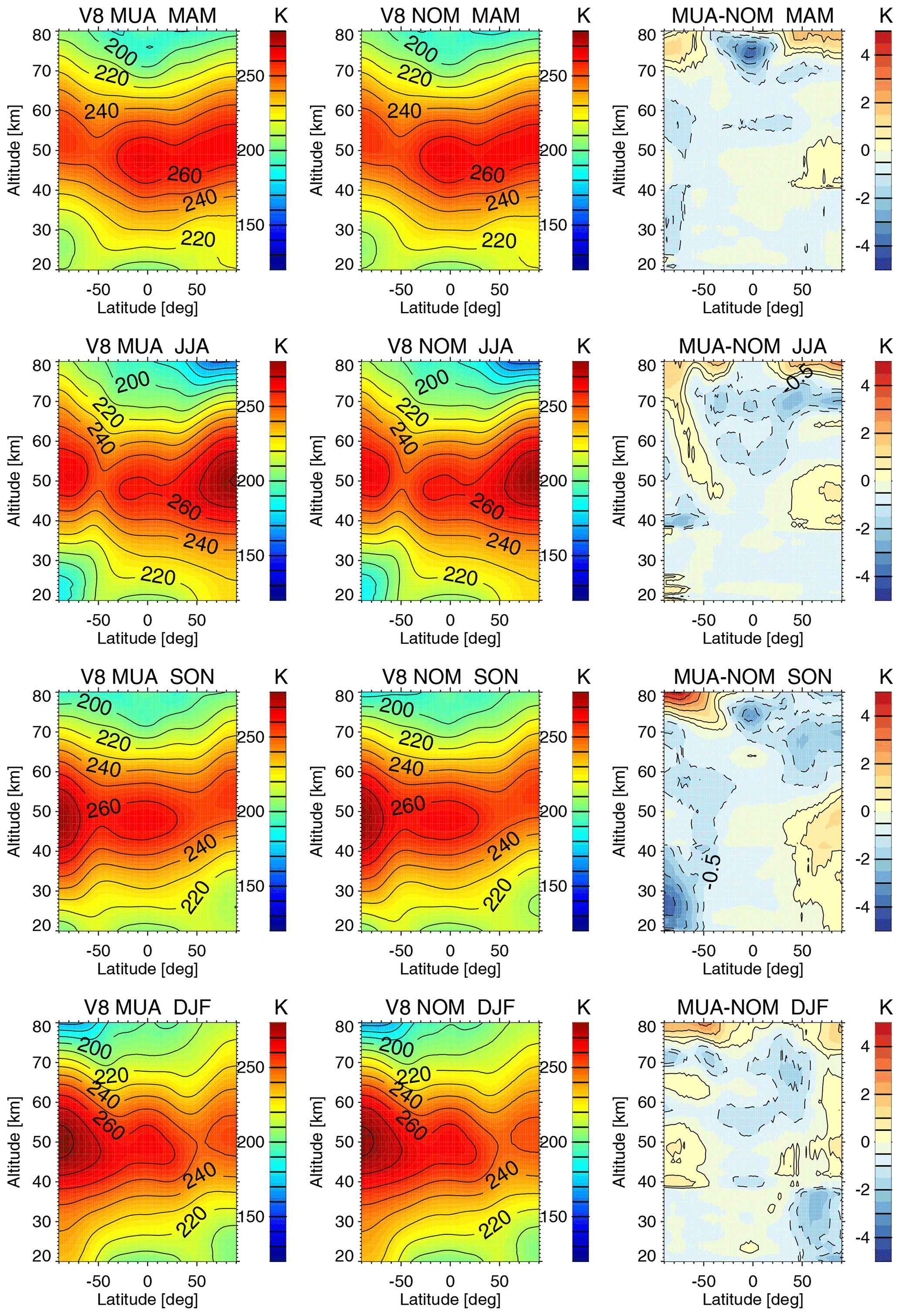
Figure 10 Comparison between 2007–2012 composites of MIPAS version 8 MA/UA (left column) and version 8 NOM (middle column) zonal mean temperatures for the four seasons. The differences are shown in the right column (contour levels are ± 0.5, ± 1, ± 2, ± 3, ± 4 and ± 5).

Here we compare 2007–2012 MA/UA and NOM version 8 temperature fields in the altitude range where they overlap to check for their consistency. Figure 10 shows 2007–2012 composites of MIPAS V8R_T_m61 (MA/UA) and V8R_T_260 (NOM) temperatures for the four seasons and their differences. MA/UA and NOM temperatures are within about 0.5 K below 70 km at all latitudes and in all seasons. Exceptions occur only for some localized areas at the polar latitudes in specific seasons, namely in the northern polar winter and at the northern polar latitudes from September to November (SON) (0.75–1.5 K differences) as well as in the lower stratosphere at southern polar latitudes also from September to November (2–3 K differences). Note that the MIPAS NOM and MA measurements are not simultaneous, so part of these small differences can be explained by the observational mismatch. These comparisons show that, in general, MIPAS version 8 MA/UA and NOM temperatures can be safely combined without special consideration.

Thermospheric temperatures can also be derived from nitric oxide spectra in a different spectral region. Version 8 temperature retrievals from NO emissions at 5.3 µm, obtained by MIPAS in the UA mode, are detailed in Funke et al. (2023). Below 110 km, the a priori temperature profiles used to derive those 5.3 µm temperatures consist of the version 8 12–15 µm UA temperatures presented here. Above 120 km, they use corrected NRLMSIS 2.0 temperature profiles as a priori temperature (Emmert et al., 2021). A merging of the two is performed at 110–120 km. Moreover, the 5.3 µm retrieved temperatures are strongly regularized towards our 12–15 µm UA temperatures below 110 km, as described in Funke et al. (2023).

We have compared the 5.3 µm with our 12–15 µm version 8 UA temperatures at 105–115 km (not shown), which is the altitude range where they concurrently provide significant information. Below 110 km, the 5.3 µm temperatures are essentially identical to our 12–15 µm temperatures for all atmospheric conditions, as expected due to the very strong regularization applied in the retrievals of the former. An exception to this occurs in the summer at latitudes poleward of 30^∘N/S, where the differences are within 5 K at 110 km. At 115 km, our 12–15 µm temperatures are generally 5–10 K higher than the 5.3 µm temperatures. The difference reaches 20–30 K for summer at latitudes poleward of 30^∘ (note that the 5.3 µm temperatures were already higher than NRLMSIS 2.0 temperatures in this altitude range; Funke et al., 2023). Importantly, the differences do not generally depend on solar illumination. Nevertheless, the differences between the 5.3 µm and the 12–15 µm temperature datasets are within our estimated systematic errors for all atmospheric scenarios.

6 Comparison with SABER

García-Comas et al. (2012) and García-Comas et al. (2014) showed comparisons of the previous MIPAS version 5 MA, UA and NLC temperatures with measurements from several instruments. In general, those MIPAS temperatures showed deviations from the other instruments within 1 K below 50 km, 2 K at 50–80 km, 4 K at 80–95 km and 5 K from 95–105 km. Exceptionally, during high-latitude summers, deviations from other instruments were less than 5 K between 65–80 km and increased to 5–10 K around the summer mesopause. MIPAS usually displayed larger vertical gradients in the thermosphere than the other instruments.

Here we compare MIPAS version 8 UA temperatures with NASA's SABER data version 2.0 (Remsberg et al., 2008; García-Comas et al., 2008; Mlynczak et al., 2022). As for MIPAS, SABER temperatures are retrieved from measurements at 15 µm considering explicit non-LTE calculations for each limb scan, although it uses a broadband channel and hence is sensitive to many CO₂ 15 µm bands. SABER temperature profiles are publicly available from 20 km to 110 km and have a 2 km vertical resolution. We selected MIPAS and SABER co-located profiles within ± 1000 km and ± 2 h UT (Universal Time). To avoid differences emanating from the coarser vertical resolution of MIPAS, especially above the stratopause, or the use of a priori information, for a given pair of MIPAS and SABER profiles, we use the corresponding individual MIPAS averaging kernel matrix (A_MIP) and a priori temperature profile (t_a,MIP) to smooth the co-located SABER profile (t_SAB), that is to say, ${\mathit{t}}_{\text{SAB,smoo}}={\mathbf{t}}_{\text{a,MIP}}+{\mathbf{A}}_{\text{MIP}}({\mathbf{t}}_{\text{SAB}}-{\mathbf{t}}_{\text{a,MIP}}$).

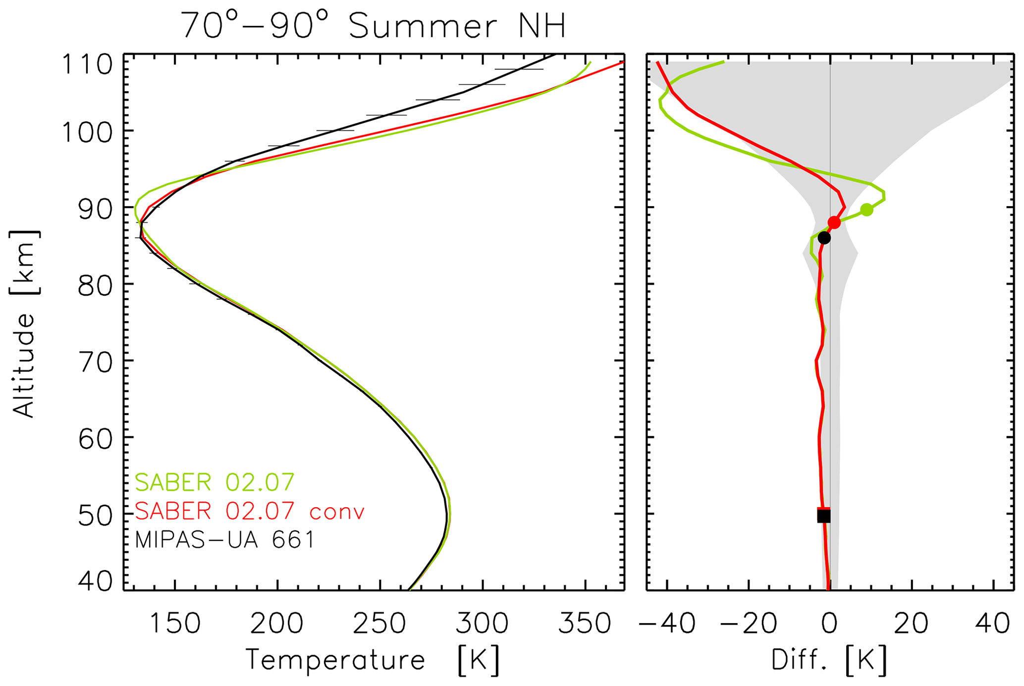
Figure 11 Effect of applying MIPAS averaging kernels to SABER co-located profiles to match MIPAS vertical resolution for the polar summer at 70–90^∘ N (black: MIPAS version 8 UA; red: SABER smoothed; green: SABER unsmoothed). The right plot shows MIPAS−SABER temperature differences. The filled squares and circles locate the stratopause and the mesopause, respectively. The shaded area shows MIPAS and SABER combined systematic errors.

Figure 11 shows the composite effect of such a smoothing on SABER profiles in the most extreme case, northern polar summer conditions. This composite is the mean difference between co-located pairs of SABER and MIPAS measurements within 70–90^∘ N in June, July and August from 2005 to 2012. Below 80 km, the composite smoothed SABER profile is not significantly different from the unsmoothed one. However, the SABER smoothed mesopause is 2 km lower and 3.5 K warmer than its unsmoothed counterpart, leading to a significantly better agreement with MIPAS. The lower thermospheric temperatures are also closer to MIPAS when the smoothing is applied. This highlights not only the well-known importance of smoothing in terms of profile-to-profile comparisons, but also for the scientific interpretation of the data, especially since the smoothing effect exhibits temporal and spatial variations.

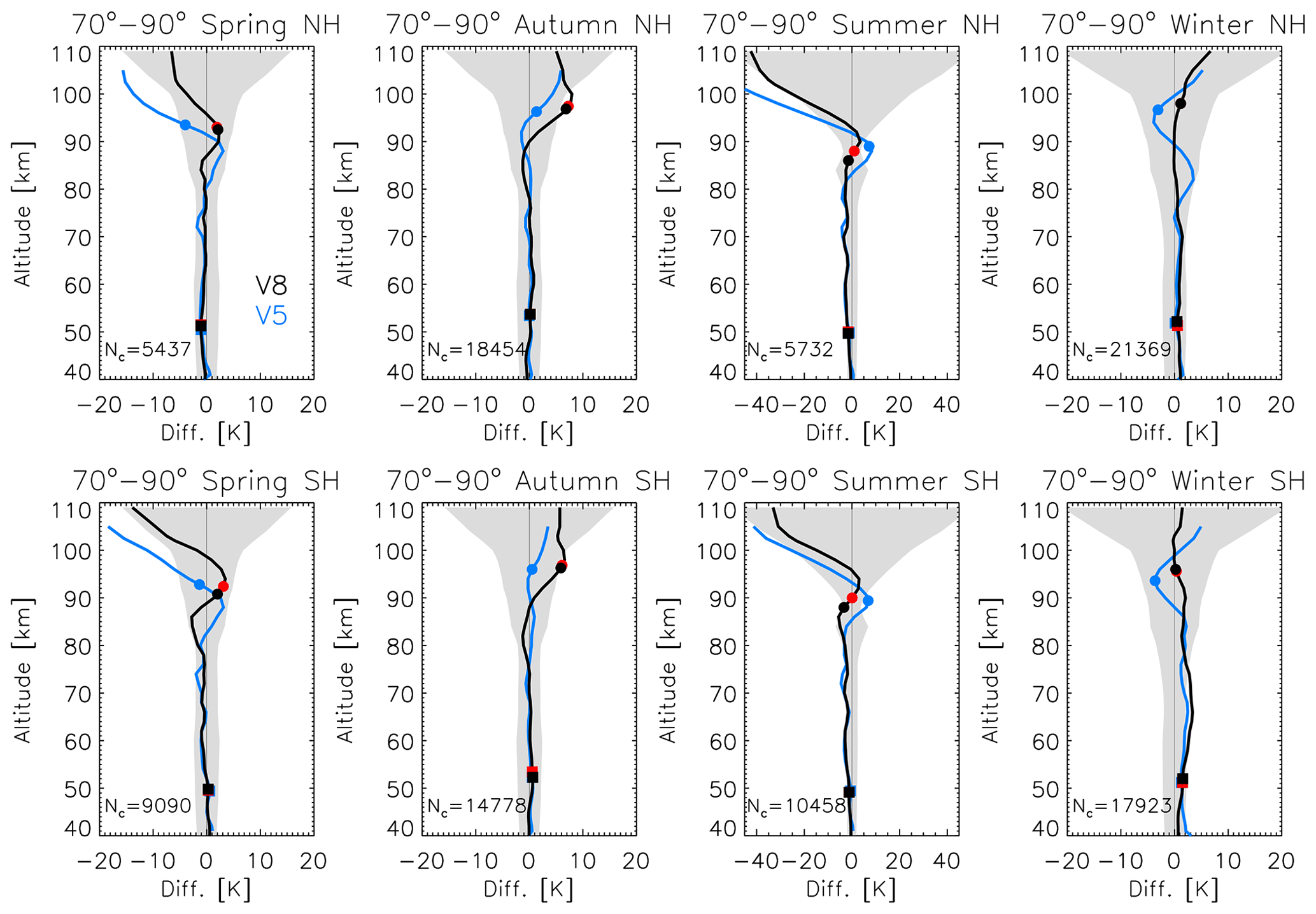
Figure 12 Co-located MIPAS−SABER differences averaged for northern (upper panels) and southern (lower panels) polar latitudes (70–90^∘averaging kernel matrix). Black: MIPAS UA version 8; blue: MIPAS UA version 5. Shaded areas show MIPAS and SABER combined systematic errors. The filled squares and circles on the lines indicate the mean altitude of the stratopause and the mesopause, respectively, also for SABER (red). N_c indicates the number of co-located pairs. Note the different x-axis scale for the summer comparison.

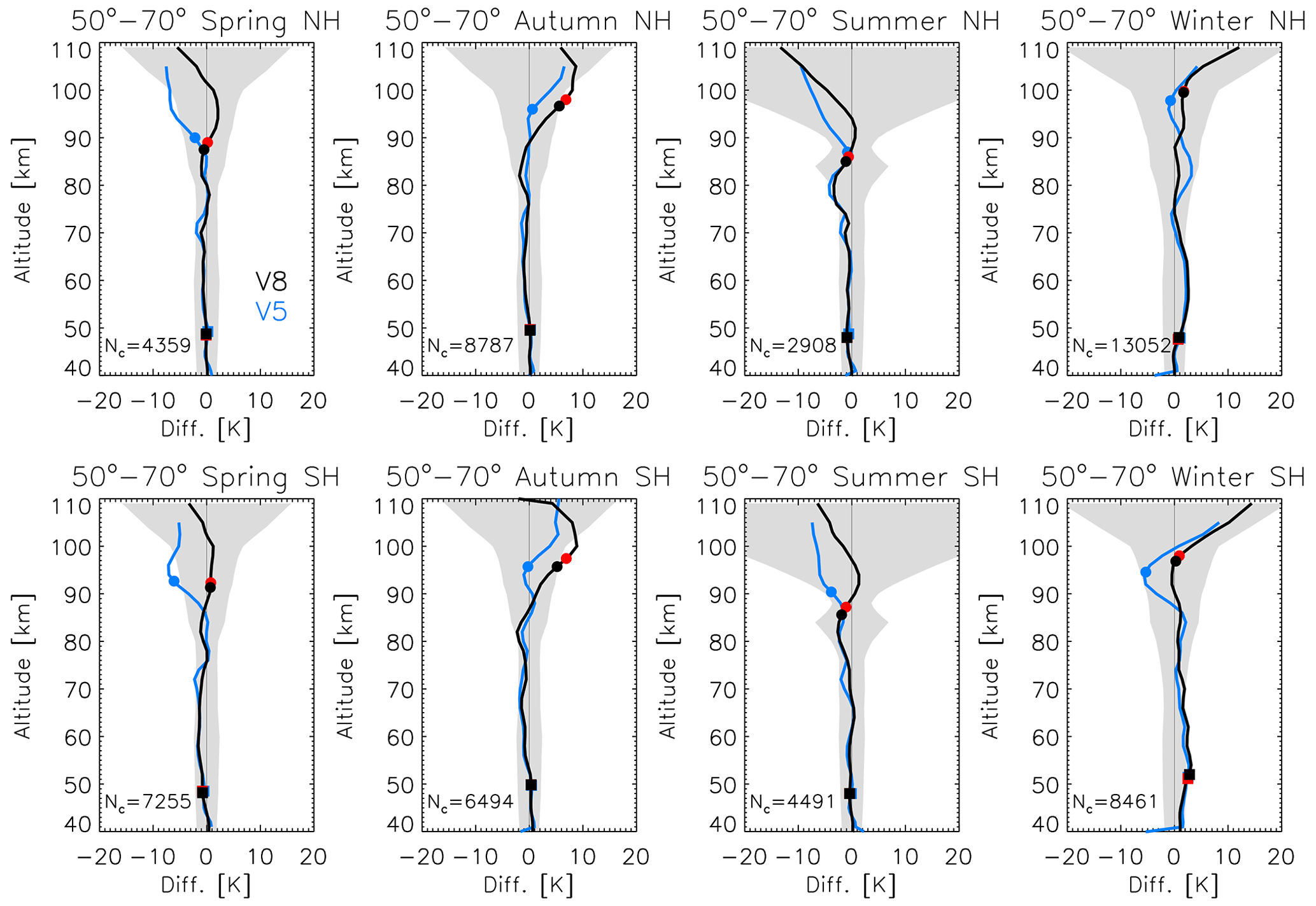
Figure 13 As Fig. 12 but for the 50–70^∘ N (upper panels) and 50–70^∘ S (lower panels) latitude boxes.

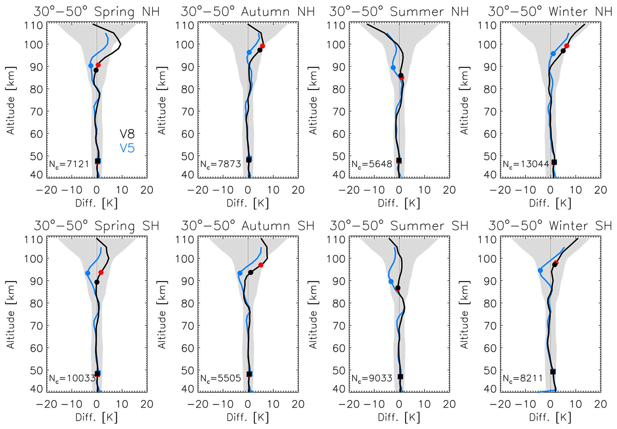
Figure 14 As Fig. 12 but for northern (30–50^∘ N; upper panels) and southern (30–50^∘ S; lower panels) mid-latitudes.

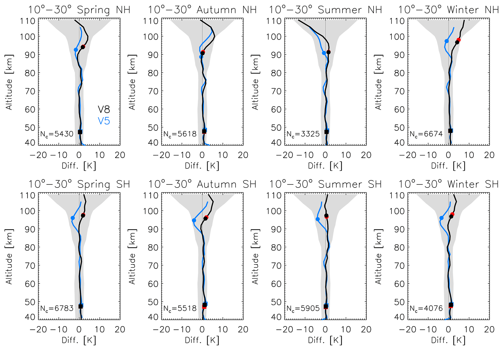
Figure 15 As Fig. 12 but for northern (10–30^∘ N; upper panels) and southern (10–30^∘ S; lower panels) tropical latitudes.

We have performed similar comparisons for five latitude boxes and the four seasons from 2005 to 2012. Figures 12–15 show the MIPAS–SABER differences averaged for northern and southern 70–90^∘, 50–70^∘, 30–50^∘ and 10–30^∘ latitude boxes, respectively. Each figure shows results for the Northern Hemisphere and the Southern Hemisphere separately. Differences with SABER are also shown for MIPAS version 5 temperatures to examine the improvements in the version presented here. The figures also depict combined MIPAS and SABER systematic temperature errors for the corresponding atmospheric conditions. These combined errors account for existing correlations between MIPAS and SABER non-LTE model uncertainties, specifically the quenching rates of CO₂(ν₂) by O, N₂ and O₂, which are set to the same values in the temperature retrievals of both instruments. We also note that SABER temperature retrievals use WACCM3 CO₂ climatologies and atomic oxygen abundance derived from SABER ozone measurements below 95 km and NRLMSISE-00 above 95 km (Mlynczak et al., 2022).

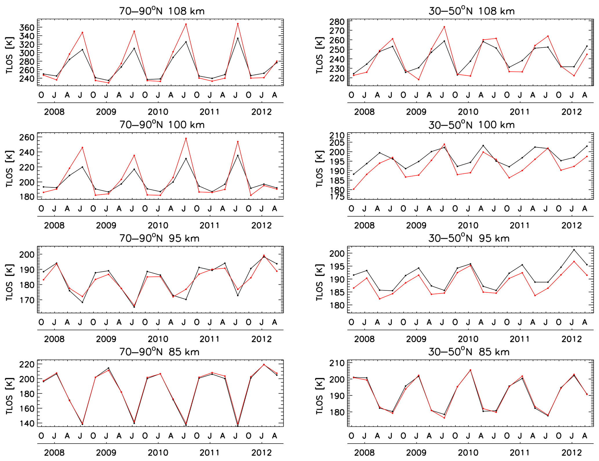
Figure 16 Seasonally averaged co-located MIPAS version 8 (black) and SABER (red) temperatures time series at 108, 100, 95 and 85 km (left: polar latitudes (70–90^∘ N); right: mid-latitudes (30–50^∘ N)).

Next, we list a selection of the most salient results:

• As a rule of thumb, MIPAS version 8 and SABER temperatures are in excellent agreement below 90 km. Temperature differences are typically within 1.5 K at these altitudes and within the combined systematic errors. In general, the comparisons with the version 8 dataset at 80–90 km improved over those with the previous version.

• There are exceptions to this rule. During summer at 70–90^∘ in the mesosphere, MIPAS temperatures are 3 K lower than SABER's, although there is still an improvement in the upper mesosphere with respect to version 5. During winter at 50–70^∘ N and S and 70–90^∘ N only in the lower mesosphere, MIPAS temperatures are 3 K higher than SABER's, but still, they are closer than in version 5 thanks to the improvements at these latitudes at 80–90 km with respect to version 5. Further, during summer at 80 km and winter in the upper stratosphere, MIPAS is 2 K warmer than SABER, as for version 5.

• The changes in MIPAS temperatures at 80–90 km from version 8 to version 5 at 70–90^∘ have reduced the differences with SABER from 6–7 K to 3–4 K in the summer and from 3–4 K to 0–1.5 K in the winter. This has further reduced the hemispheric asymmetry of the differences.

• Version 8 temperatures are higher than in version 5 at all altitudes above 90 km, except above 100 km in the polar winters. This leads to improvements in the comparisons with SABER in many cases, but not always. Comparisons with the new MIPAS version improve significantly in summer at latitudes equatorward of 70^∘ N/S, where the differences with SABER are within 3–4 K at 90–100 km, 4–6 K at 100–110 km in the Southern Hemisphere and 5–10 K at 100–110 km in the Northern Hemisphere. The improvement is not sufficient to bring the MIPAS and SABER polar summer temperatures closer than 10 K above 95 km. However, the disagreement between the two instruments generally falls within the range of the combined retrieval error.

• The typically higher MIPAS temperatures above 90 km in version 8 also lead to improvements in the comparisons with SABER at 90–100 km in the winter, particularly in the Southern Hemisphere and also at high latitudes (differences within 3–4 K). They also further lead to better agreement in spring at latitudes poleward of 30^∘ S in the Southern Hemisphere (differences within 3–4 K) and poleward of 50^∘ N in the Northern Hemisphere (differences within 3–5 K).

• However, the comparisons of MIPAS version 8 temperatures with SABER observations deteriorate at 100–110 km elsewhere in spring and also everywhere in autumn and winter (except at latitudes of 70–90^∘ N and S). In these cases, the differences increase from 1–6 K in version 5 to 4–9 K in version 8. With the exception of the polar autumn at 100 km, they still fall within the estimated combined errors.

• At altitudes ranging from 100 to 110 km and latitudes ranging from 70 to 90^∘ during the winter, version 8 temperature differences with SABER are less than 1 K in the Southern Hemisphere (significantly improving the agreement with respect to that with the previous MIPAS version) and 2–6 K in the Northern Hemisphere.

• There are slight changes in the MIPAS–SABER differences from one hemisphere to the other, but it is difficult to glimpse any systematic behavior. The most striking examples of asymmetry are the summers at latitudes poleward of 30^∘ N/S above 95 km.

Beyond this, we have also compared co-located MIPAS and SABER time series. For this purpose, MIPAS averaging kernels and a priori information were also applied to the SABER profiles. Figure 16 shows such comparisons for northern polar and mid-latitudes for selected altitudes (note the different scales in the abscissas). We started the time series at the end of 2007 because MIPAS data are not available before for some seasons.

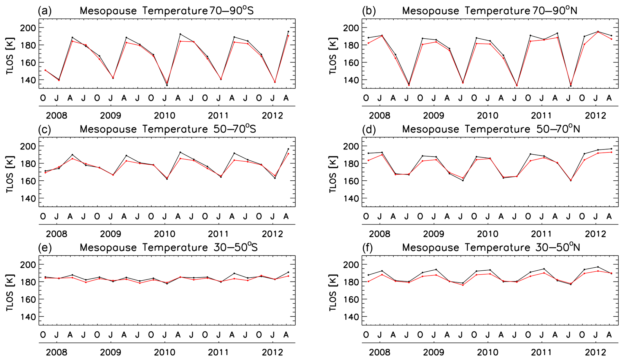
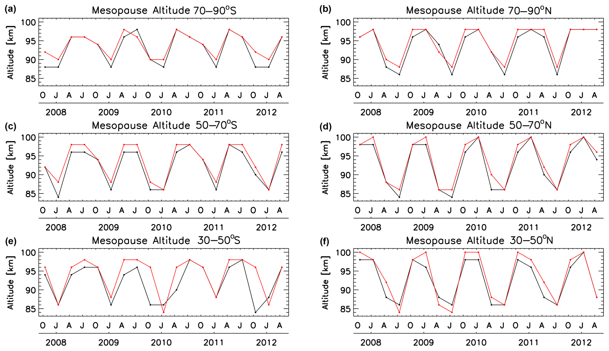
Figure 17 Comparison of seasonal time series of co-located MIPAS UA version 8 (black) and SABER (red) mesopause temperatures averaged over six latitude boxes (a, c, e: Southern Hemisphere; b, d, f: Northern Hemisphere; from top to bottom: 70–90^∘, 50–70^∘, 30–50^∘).

The agreement at the lowermost altitude shown (85 km) is remarkable. Temperatures agree within 1–2 K each season and each year. Both instruments exhibit similar peak-to-peak amplitudes (60–80 K in the poles, 20–25 K at mid-latitudes), which vary similarly from year to year. At polar latitudes, the agreement at 95 km is somewhat worse (peak-to-peak amplitudes are 5 K larger for MIPAS). However, the seasonal behavior of the differences is more or less consistent from year to year. At 95 km at mid-latitudes, MIPAS temperatures are always 2–3 K higher than SABER, leading to a similar seasonal variation but shifted.

At 100 km, MIPAS northern polar temperatures are lower than SABER in all winters and higher in all summers, and winter–summer differences change very slightly from year to year. This means that while MIPAS provides peak-to-peak amplitudes between 30 and 45 K, SABER provides values between 50 and 75 K. A similar behavior is also observed at mid-latitudes but with smaller amplitudes (10 K for MIPAS and 15 K for SABER), both instruments showing a rather small year-to-year variation.

At the uppermost altitude shown in Fig. 16 (108 km), MIPAS polar winter temperatures are 35–40 K lower than those from SABER, while they are 5–10 K warmer in the summer. This leads to peak-to-peak amplitudes of 90–100 K for MIPAS but 120–140 K for SABER. However, the difference between the instruments here does not vary from year to year. For mid-latitudes, the behavior is similar but less pronounced, with MIPAS yielding 20–25 K amplitudes and SABER 40–50 K amplitudes.

Figure 18 As Fig. 17 but for the mesopause altitude seasonal time series.

Given its relevance for atmospheric dynamics, we also examined the MIPAS mesopause temperature and altitude time series together with those from SABER (Figs. 17 and 18). The identification of the mesopause at lower latitudes becomes difficult due to the temperature double-peak structure in the upper mesosphere. Therefore, we restricted the comparison to latitudes higher than 30^∘ N/S.

MIPAS and SABER mesopause temperature and altitude time series at 70–90^∘ N and S and 50–70^∘ N and S show similar behavior for both hemispheres. MIPAS version 8 high-latitude winter, spring and summer mesopause temperatures are in excellent agreement with SABER (1–2 K difference), with both instruments exhibiting similar coolest temperatures during the polar summers (135–140 K in the Southern Hemisphere and, generally, 5 K colder in the Northern Hemisphere). We recall that the agreement between MIPAS and SABER temperatures in spring and summer has typically improved from MIPAS version 5 to version 8 (Fig. 12), including the year-to-year variability. This was not the case for autumn, where the mesopause co-located temperatures in version 8 increased from version 5, yielding a 5 K warmer autumn mesopause than in SABER observations. This differential seasonal behavior causes a 5 K larger autumn-to-winter mesopause temperature change and also an increased annual oscillation in MIPAS as compared to SABER.

Both MIPAS and SABER show very small seasonal mesopause temperature variations at 30–50^∘ S (5–7 K peak-to-peak variations), barely changing from year to year for the time range of our comparison. The agreement is slightly worse at 30–50^∘ N, where MIPAS also measures a 5 K warmer mesopause during the autumn and the winter, as for the higher latitudes.

The comparisons of MIPAS version 8 and SABER mesopause altitudes (Fig. 18) typically show good agreement, with very similar seasonal variations. Minimum mesopause altitudes occur during summer at all latitudes, generally at 86 km in MIPAS and 88 km in SABER. The lowest co-located average mesopause altitudes measured by these two instruments were 84 km (at 50–70^∘ N in 2008 and 2009 by MIPAS and 30–50^∘ N also in 2008 and 2009 by SABER). Particularly noticeable is the often parallel variation in MIPAS version 8 and SABER mesopause altitudes along the time series, indicating a systematic 2 km lower mesopause in MIPAS data. An exception to this behavior occurs at 30–50^∘ N, where the MIPAS autumn and summer mesopause is higher than that of SABER. We note that, except in the winters and also at low latitudes, the MIPAS mesopause in version 8 is at lower altitudes than in version 5 (black and blue circles, respectively, in Figs. 12–15). The changes are at most −4 km during the summers, resulting in general better agreement with SABER in MIPAS version 8.

7 Conclusions

Following the release of version 8.03 of the calibrated MIPAS spectra by ESA, we have reprocessed the measurements in MA, UA and NLC modes to provide the community with version 8 of the IMK–IAA temperature and tangent altitude correction dataset derived from 12–15 µm emissions. The configuration of the IMK–IAA retrieval processor for this temperature version does not differ from that used for the inversion of the NOM data presented by Kiefer et al. (2021), except that here we took into account the non-LTE explicitly calculated for each limb scan according to the sophisticated scheme described in Funke et al. (2012), which is generally of importance above the mid-mesosphere. The use of the nearly identical retrieval configuration results in an excellent consistency between the IMK–IAA version 8 NOM and MA/UA/NLC temperature products.

In addition to the improved calibrated spectra, the upgrades to the MA/UA/NLC temperature retrievals in version 8 with respect to the preceding IMK–IAA version 5 are (1) more realistic atomic oxygen abundances, derived from WACCM4 abundances at MIPAS geolocations bias-corrected according to MIPAS version 5 O₃ and O climatology; (2) more realistic carbon dioxide abundances, extracted from the SD-WACCM4 model; (3) the 2016 HITRAN spectroscopy; (4) an improved spectral shift retrieval; (5) the continuum retrieval up to 58 km; (6) the consideration of an altitude-dependent radiance offset retrieval; (7) the use of wider microwindows above 85 km in order to capture the offset; (8) a higher accuracy in the forward model calculations; (9) a new a priori temperature; (10) improved temperature horizontal gradient retrievals, where we derive a linear correction to a full 3D temperature field; and (11) the use of interfering species abundances retrieved from the MIPAS IMK–IAA retrieval version 5, where available.

These upgrades in version 8 result in temperature changes relative to version 5 of less than 0.5 K below 70 km; 1–3 K oscillating temperature changes at low to mid-latitudes from 70 to 105 km; a vertically shifted mesopause at high-latitudes, resulting in maximum differences of 3 K in polar winter and 7 K differences in polar summer; and 5–25 K higher temperatures at 105–115 km.

The MIPAS MA/UA/NLC IMK–IAA temperature dataset is reliable for scientific analysis in the full measurement vertical range for MA (18–102 km) and NLC (39–102 km) and from 42 to 115 km for UA measurements. Temperatures derived from 12–15 µm emissions provided in version 8 IMK–IAA dataset do not contain atmospheric information and are not usable above 115 km. The vertical resolution of the temperature profiles is 3 km at altitudes below 50 km, 3–5 km at 50–70 km, 4–6 km at 70–90 km, 6-1-0 km at 90–100 km and 8–11 km at 100–115 km.

We have estimated the random and systematic error components for 35 representative atmospheric conditions, covering day and night and polar, middle and tropical latitudes of the Northern Hemisphere and the Southern Hemisphere. The error sources considered are the measurement and the radiance offset noises; the uncertainties in the instrument line shape, gain calibration, spectral shift, CO₂ spectroscopy, and CO₂ and O abundances; and uncertainties in the collisional rates of vibrational exchange of υ₂ quanta between CO₂ molecules and the quenching of the CO₂(υ₂) states through collisions with atomic oxygen, molecular nitrogen and molecular oxygen.

The main source of MIPAS random temperature errors is the measurement noise. The noise errors are less than 1 K at altitudes below 60 km, 1–3 K at 60–70 km, 3–5 K at 70–90 km, 6–8 K at 90–100 km, 8–12 K at 100–105 km and 12–20 K at 105–115 km. Besides the measurement noise, the random component generated by the CO₂ abundance and the CO₂(υ₂)–O quenching uncertainties are significant in the lower thermosphere, reaching 3–7 K and 5–10 K at 105–115 km.

The systematic temperature errors below 75 km are driven by uncertainties in the CO₂ spectroscopic data, resulting in errors smaller than 0.7 K below 55 km, 1 K at 60–70 km and smaller than 0.5 K above those altitudes. Above 80 km, the systematic temperature errors are driven by uncertainties in the non-LTE model parameters, namely the collisional rates and the atomic oxygen and CO₂ abundances. The non-LTE uncertainties generally lead to systematic errors smaller than 0.5 K below 75 km (80 km for the polar winter), 1 K at 80 km (2 K in the polar winter), 3 K at 95 km (5 K in the polar summer), 6–8 K at 100 km (15 K in the polar summer), 10–20 K at 105 km (30 K in the polar summer) and 20–30 K at 115 km (50 K in the polar summer). These errors are dominated by the contribution of the CO₂(υ₂)–O quenching uncertainty. The CO₂ uncertainties lead to typical 1–2 K systematic temperature errors at 95–105 km and 7–10 K at 110–115 km. In the mid-latitude and polar summer, these values increase to 2–7 K at 95–105 km and about 20 K at 115 km.

We have conducted comparisons between MIPAS version 8 temperatures and co-located measurements from the SABER instrument. There is excellent agreement below 90 km, with differences typically within 1.5 K, except for a few cases such as the polar summer mesosphere and the high-latitude winter lower mesosphere, where differences are within 3 K. The differences between the datasets above 90 km are dependent on the season and latitude. Generally, they are within 1–3 K at 90–95 km, 1–5 K at 95–100 km, 1–8 K at 100–105 km and 1–10 K above. However, an exception to this occurs during the polar summer above 95 km, where MIPAS and SABER differences are significantly larger (8–35 K). These differences can be roughly explained by the combined retrieval errors in both instruments, except for the polar latitudes during autumn at 100 km and the lower mesosphere in the Southern Hemisphere polar winter. The comparisons between SABER and MIPAS version 8 showed an overall improvement over those with version 5, particularly at altitudes above 90 km, except for the lower thermosphere during autumn.

Our systematic error budget for temperatures highlights the need to reduce the current uncertainties in the non-LTE kinetic parameters, in particular in the CO₂(ν₂)–O collisional rate (k_O) and the carbon dioxide concentrations in the upper mesosphere and lower thermosphere. Improved measurements of the rate of CO₂(v₂) quenching by N₂ and O₂ (k_air) and the rate of ν₂-quanta exchange between CO₂ molecules (k_vv) would also be beneficial. Finally, a better characterization of the instrument line shape would have also been desirable.

Appendix A: Temperature error values

We include in this appendix the tables with the error values corresponding to Figs. 5–7 and discussed in Sect. 3. We recall that the Supplement of this paper contains plots and tables with the error estimations for 34 representative atmospheric scenarios, corresponding to day and night of spring, summer, autumn and winter conditions at polar latitudes, at mid-latitudes and in the tropics.

Table A1 Temperature error budget for the selected solstice atmospheric scenarios at polar latitudes shown in Fig. 5. All uncertainties are 1 σ. The “Mean” column refers to the mean temperature. “NLTE” and “Spectro” correspond to errors due to non-LTE and spectroscopy uncertainties, respectively. “Random” and “Syst” refer to total random and systematic temperature errors, respectively.

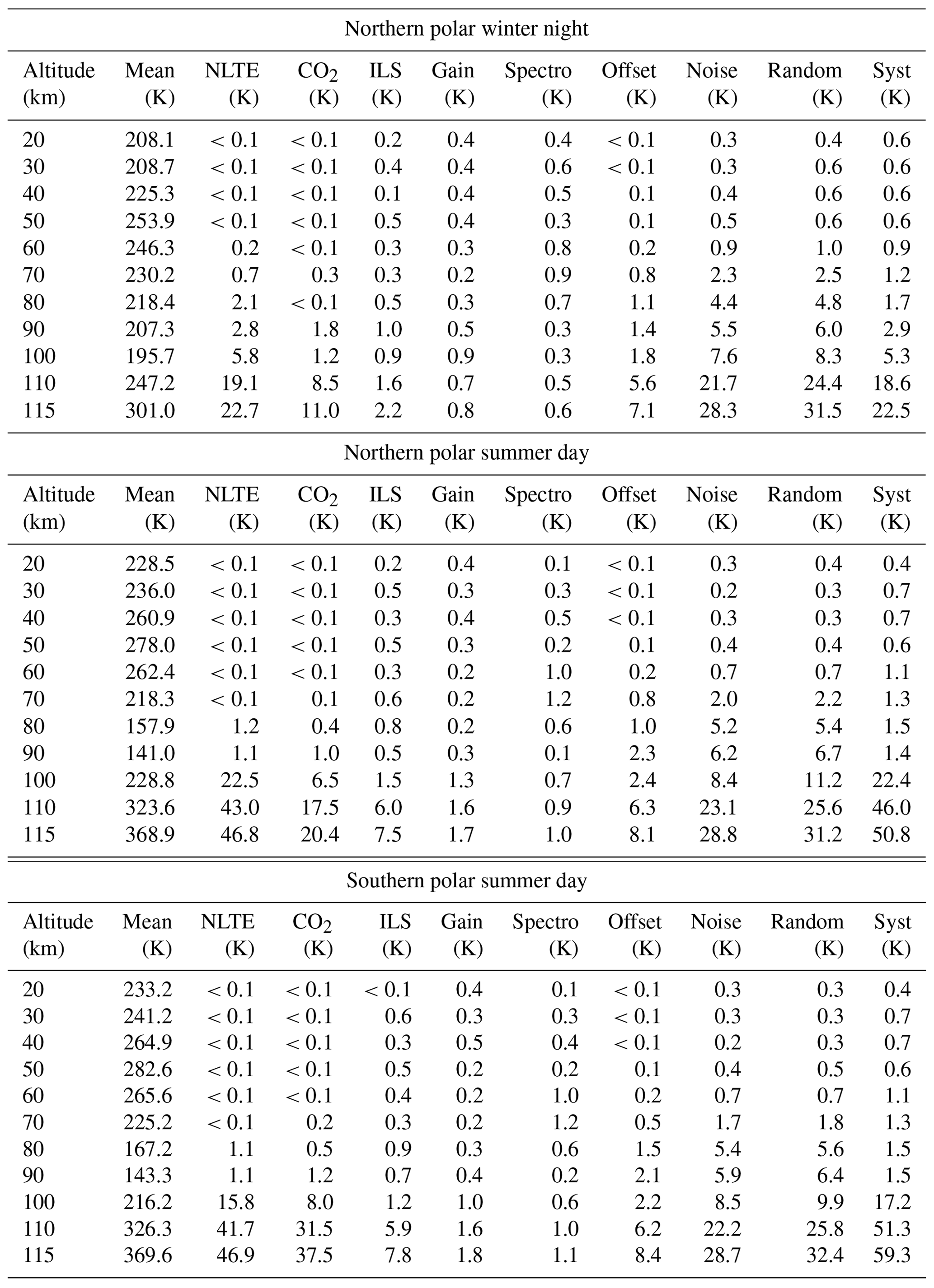
Table A2 Temperature error budget for the selected solstice atmospheric scenarios at mid-latitudes shown in the left column of Fig. 6. All uncertainties are 1 σ.

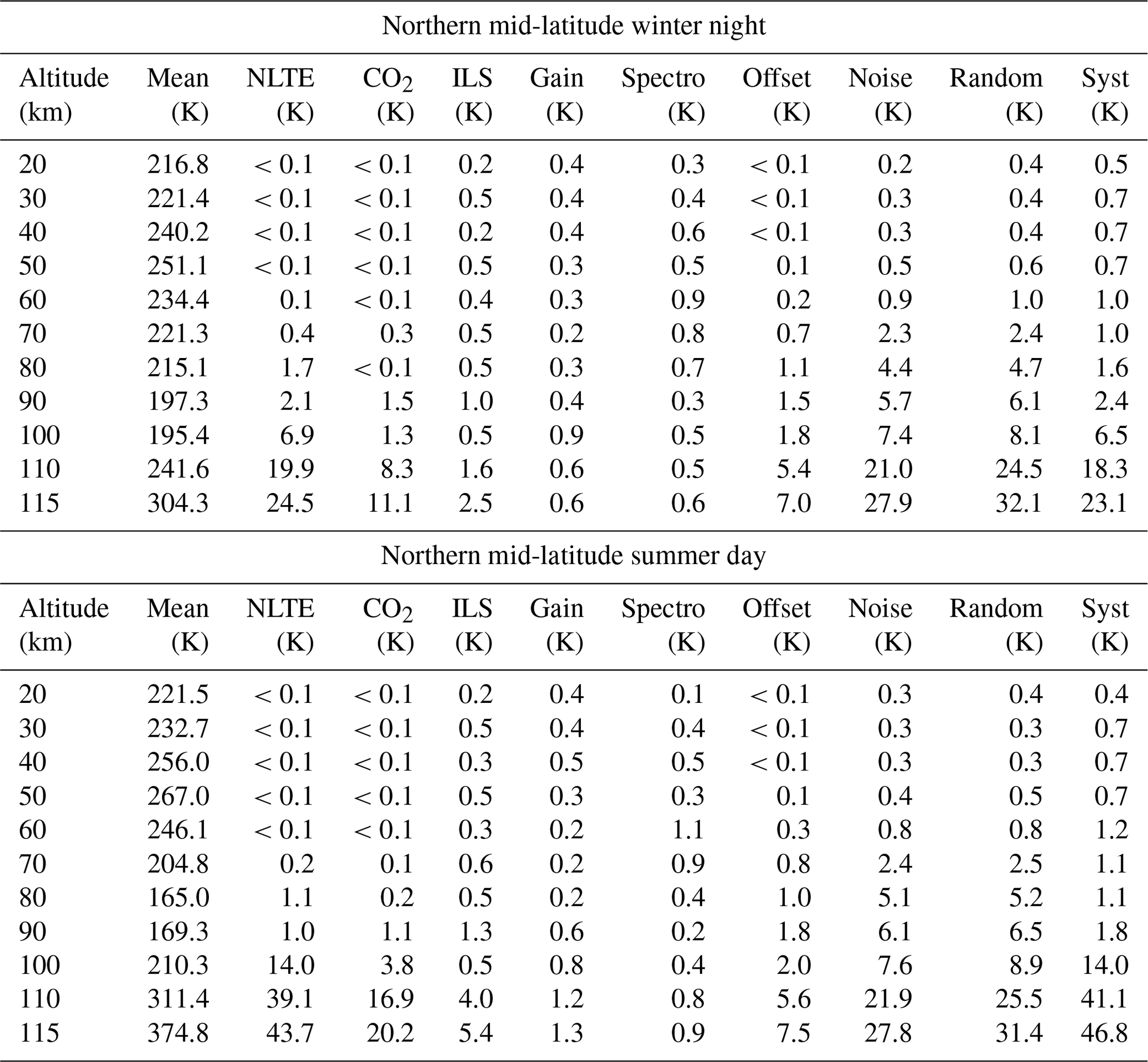
Table A3 Temperature error budget for selected equinox atmospheric scenarios at mid-latitudes shown in the right column of Fig. 6. All uncertainties are 1σ.

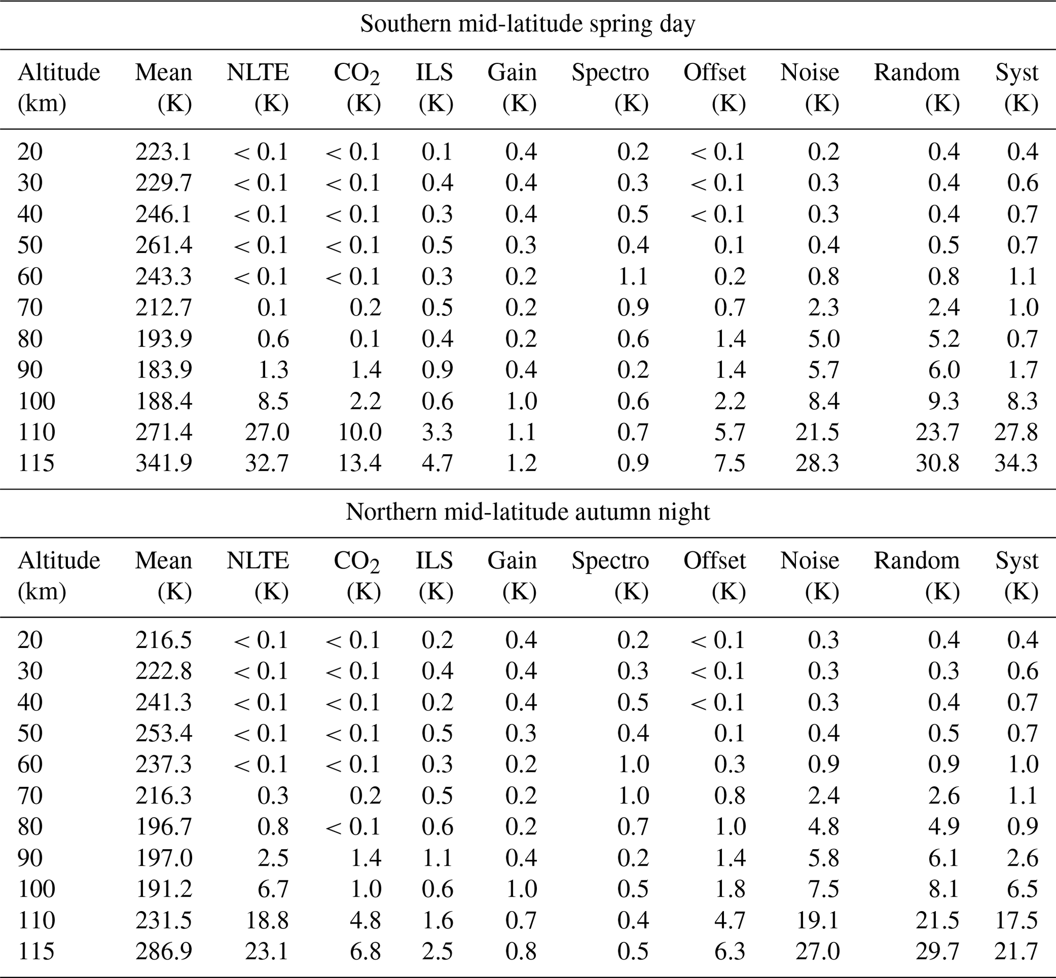
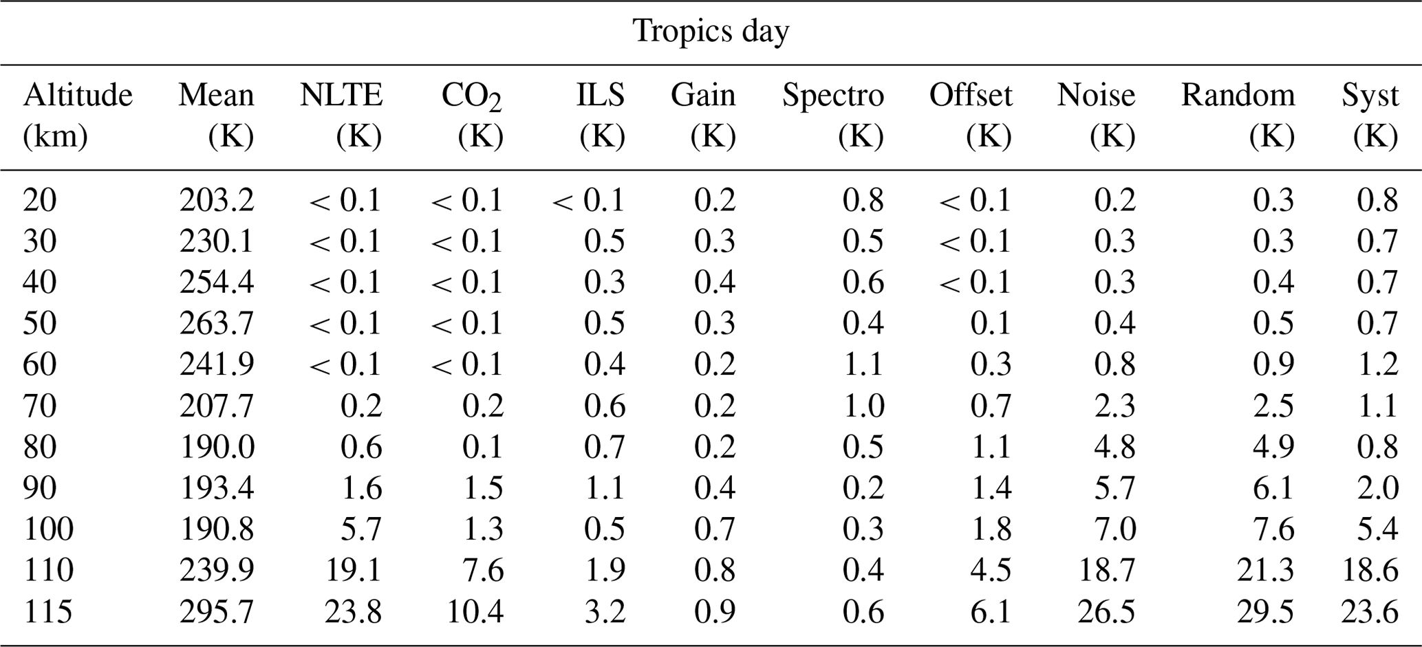
Table A4 Temperature error budget for the tropics during the day, also shown in Fig. 7. All uncertainties are 1 σ.