Spectral analysis approach for assessing the accuracy of low-cost air quality sensor network data

Extensive monitoring of particulate matter (PM) smaller than 2.5 µm, i.e., PM_2.5, is critical for understanding changes in local air quality due to policy measures. With the emergence of low-cost air quality sensor networks, high spatiotemporal measurements of air quality are now possible. However, the sensitivity, noise, and accuracy of field data from such networks are not fully understood. In this study, we use spectral analysis of a 2-year data record of PM_2.5 from both the Environmental Protection Agency (EPA) and PurpleAir (PA), a low-cost sensor network, to identify the contributions of individual periodic sources to local air quality in Chicago. We find that sources with time periods of 4, 8, 12, and 24 h have significant but varying relative contributions to the data for both networks. Further analysis reveals that the 8 and 12 h sources are traffic-related and photochemistry-driven, respectively, and that the contributions of both these sources are significantly lower in the PA data than in the EPA data. The presence of distinct peaks in the power spectrum analysis highlights recurring patterns in the air quality data; however, the underlying factors contributing to these peaks require further investigation and validation. We also use a correction model that accounts for the contribution of relative humidity and temperature, and we observe that the PA temporal components can be made to match those of the EPA over the medium and long term but not over the short term. Thus, standard approaches to improve the accuracy of low-cost sensor network data will not result in unbiased measurements. The strong source dependence of low-cost sensor network measurements demands exceptional care in the analysis of ambient data from these networks, particularly when used to evaluate and drive air quality policies.

1 Introduction

Air pollution is one of the world’s leading risk factors for disease and premature death. An estimated 16 % of total global deaths in 2015 can be attributed to diseases caused by air pollution (Landrigan et al., 2018). Of particular concern is the mass concentration of particulate matter (PM) smaller than 2.5 µm, i.e., PM_2.5, or fine particles. Exposure to PM_2.5 has been directly correlated with diseases such as respiratory diseases and even mortality (Li et al., 2018; Xing et al., 2016; Samoli et al., 2005; Ostro et al., 2006; Lewis et al., 2005). The high health impact of PM_2.5 is because of its ability to penetrate deep into the lungs and because its composition is often carcinogenic (Li et al., 2014). The European Study of Cohorts for Air Pollution Effects (ESCAPE) shows that exposure to high PM_2.5 concentrations is linked to a risk of developing lung cancer (Raaschou-Nielsen et al., 2013). In addition to chronic diseases, exposure to PM_2.5 might also impact our response to acute diseases such as COVID-19 (Wu et al., 2020; Zhou et al., 2021; Mondal et al., 2022; Chaipitakporn et al., 2022). Accurate knowledge of PM_2.5 exposure and efforts to mitigate it are critical to protecting public health.

In the United States, the Environmental Protection Agency (EPA) monitors air quality by measuring regulated or criteria pollutants, including ambient PM_2.5 concentrations using Air Quality Monitoring Stations (AQMSs). The PM_2.5 measurements are made using a range of instruments classified as federal reference methods (FRMs) or federal equivalent methods (FEMs) (Noble et al., 2001). FRMs refer to the specific monitoring methods that have been designated by the EPA as the reference standard for measuring air pollutants, while FEMs refer to alternative monitoring methods that have been deemed equivalent to the FRM methods by the EPA. The two methods may utilize different instruments or measurement techniques but have demonstrated comparability in accuracy and reliability. The strict maintenance and calibration routines followed in these stations ensure high-quality data and comparability between different locations (Castell et al., 2017). Even in the US, with over 5000 AQMSs, the geographic coverage of these monitoring sites is inadequate. The siting of AQMSs is often biased towards populated areas, disadvantaging smaller cities and underdeveloped regions (Ardon-Dryer et al., 2020). Even in populated areas, the limited number of sites does not capture the high spatial variation in PM_2.5 concentrations that are likely, resulting in an incorrect estimate of exposure and the resultant health effects (Wang et al., 2015).

For accurate exposure assessment, an air quality monitoring network providing measurements at high spatiotemporal resolution is required. To address this need, researchers, communities, organizations, and individuals have been deploying low-cost air quality sensors that provide air quality data at a granular level not possible with the EPA AQMSs (Commodore et al., 2017; Woodall et al., 2017). One of these networks is composed of sensors from PurpleAir (PA). The PA sensing platform incorporates a pair of Plantower PMS5003 low-cost sensors, which use laser light-scattering techniques to determine ambient aerosol concentrations. A PMS5003 reports a variety of particle concentration metrics, including PM₁, PM_2.5, and PM₁₀ (Sayahi et al., 2019; Ouimette et al., 2022; He et al., 2020). The PA provides two PM_2.5 values labeled cf_1 (higher correction factor) or cf_atm (atmosphere). The two values have different correction factors that convert the sensor light-scattering measurements to PM. For a relative humidity (RH) of less than 70 %, both values yield similar results for a PM_2.5 of less than 25 µg m⁻³. Outside this range, cf_atm and cf_1 start to disagree (Barkjohn et al., 2021). It is important to note that the specific algorithm employed by PA to convert Plantower data into mass concentration, whether using cf_1 or cf_atm correction factors, has not been publicly disclosed (Ouimette et al., 2022). PA sensors also have two channels, namely A and B, that measure the exact same PM measurements. These two channels allow for the robustness of data collection by minimizing any data noise, loss of data due to sensor failure, or measurement error due to sensor electronic issues (PurpleAir, 2020). While the low-cost sensors have the advantage of deployment ease, their accuracy and precision are variable (Kuula et al., 2017).

PA provides two PM_2.5 values, labeled cf_1 (higher correction factor) or cf_atm (atmosphere). The two values have different correction factors that convert the sensor light-scattering measurements to PM. For RH less than 70 %, both values yield similar results for PM_2.5 less than 25 µg m⁻³. Outside this range, cf_atm and cf_1 start to disagree (Barkjohn et al., 2021). It is important to note that the specific algorithm employed by PA to convert Plantower data into mass concentration, whether using cf_1 or cf_atm correction factors, has not been publicly disclosed (Ouimette et al., 2022).

The various PM sensors used in low-cost monitors are all subject to biases and calibration dependencies, with some factors accounted for with moderate success (e.g., meteorology, age of sensor) and others poorly (e.g., aerosol source, composition, refractive index) (Giordano et al., 2021). The PA sensor measurements are often calibrated or corrected by co-location with a reference monitor at a regulatory site (Wallace et al., 2021; Stavroulas et al., 2020; Kelly et al., 2017). Additionally, researchers have developed correction models to account for the impact of environmental conditions on sensor performance (Barkjohn et al., 2021; Ardon-Dryer et al., 2020). The deployment of PA sensors has resulted in expanding the availability of PM_2.5 data and enabling a range of studies, including validation of high-resolution, large-scale regional modeling efforts (Bi et al., 2020) and understanding of the impact of wildfire smoke on local and regional air quality (Gupta et al., 2018).

Co-locating low-cost sensors with reference monitors provides a fast way for their calibration. Typically, this is done by co-locating the sensors for a period of time and then determining a scaling factor or equation based on a regression analysis. The time period for co-location is generally chosen to be around days to weeks, and this allows for the calibration to be independent of data noise. The selection of the calibration time period can, however, bias the sensor data to be most sensitive to sources primarily responsible for pollutant concentration variability in that time period. Sources with shorter time periods, relative to the calibration period, are averaged out and inadequately accounted for in the calibration. Thus, longer timescale events are completely lost in the calibration process.

Published studies on low-cost sensors have observed some of the abovementioned problems. The response characteristics of low-cost sensors are seen to be different from those advertised by their manufacturers, possibly because the aerosol size distributions and compositions differ with location (Kuula et al., 2020; Tryner et al., 2020). As an example, low-cost sensor data are seen to be in better agreement with reference monitors at locations with low traffic than those at high-traffic locations (Castell et al., 2017). To improve the quality of the reported data from low-cost sensor networks, we need to establish ideal field calibration principles for these units. For this, frequency-based methods that have been previously used in air quality to find prominent temporal components can be used (Hies et al., 2000; Marr and Harley, 2002; Choi et al., 2008; Tchepel and Borrego, 2010). Time series decomposition using low-pass filters can identify pollution sources that account for most of the measurement variation (Zhang et al., 2018; Bai et al., 2022). Here, using frequency-based analysis, the dependence of low-cost sensor PM_2.5 measurement accuracy on the calibration period will be established.

For this work, we chose our study area to be Cook County, IL, which includes the city of Chicago and has a total population of nearly 10 million. Cook County is a major transportation hub lying at the crossroads of the country's rail, road, and air traffic, and it is an important industrial center; thus, there are a number of emission sources within the area. Despite a baseline long-term trend of improving air quality in Chicago, recent years show a worsening trend. PM_2.5 concentrations have nearly doubled since 2017, rising from 6.7 µg m⁻³ in 2017 to 12.8 µg m⁻³ in 2019, exceeding the U.S. EPA air quality standards (12 µg m⁻³) (IQAIR, 2020). The likely reason for the increase in PM_2.5 levels is the associated increase in emissions from mobile sources in recent years (Milando et al., 2016). The changing air pollution levels have increased public interest in air quality monitoring, particularly using low-cost sensor networks. For the time period starting in May 2018, the PurpleAir network in Chicago and its surrounding neighborhoods has increased from a few sensors to more than 30 sensors now.

In this study, we used PM_2.5 data from EPA sites and PA sensors located in Cook County, IL, to understand differences in their data as a function of sensor location and time. Using spectral theory, we extracted temporal signatures of the EPA and PA data and analyzed their differences as a function of the time period to determine the effectiveness and limitations of the current approach to correct low-cost sensor data to match the EPA data. The results of this analysis will help us understand biases in the data from low-cost sensors such as PA networks and provide guidance in devising new approaches to field-calibrate data from these sensors.

2 Materials and methods

2.1 Data collection and preprocessing

Cook County, IL, has 14 EPA air quality monitoring sites providing data on criteria pollutants, including ambient PM_2.5 concentrations (EPA, 2021). Hourly PM_2.5 measurements from the EPA are available at 7 out of 14 monitoring sites in Cook County, IL. The PA network in Cook County consists of more than 30 PA low-cost sensors that currently provide PM_2.5 data (PA, 2021). Our analysis was conducted using data from a time period of October 2019 to September 2021. For this time period, hourly PM_2.5 data were only available at 10 out of 30 PA sensors. Further, after eliminating sites with more than 20 % missing data, our analysis could only use data from five EPA sites and nine PA sensors, as shown in Fig. 1 and Table S1 in the Supplement.

Figure 1 (a) EPA and PA sampling locations. (b) Population density (population per square mile) in the block defined by the U.S. Census Bureau in Cook County, IL. Basemap used from ESRI (ESRI, 2021).

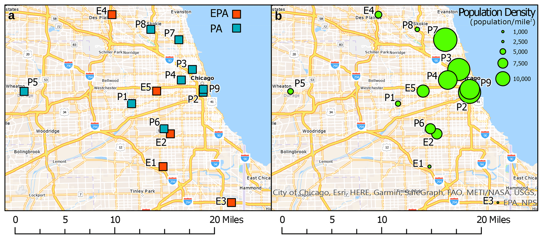
It was observed that PA data included some outliers with very large PM_2.5 concentrations, which are likely erroneous data. To eliminate these outliers from our analysis, we chose a data range of [0,70] µg m⁻³ as valid data (Ardon-Dryer et al., 2020). In Fig. 1a the sampling locations of EPA and PA are plotted on the map with the population density around the sampling locations in Fig. 1b. The population density in census blocks, as defined by the U.S. Census Bureau (Bureau, 2021), was calculated using ArcGIS Pro 2.8. From a simple analysis of the siting of sensors, it is clear that more than 60 % of the PA sensors are located in urban areas where the average population density is more than 5000, exceeding that of the EPA sites except for EPA site E2.

2.2 Standard correction model

It has been established that low-cost sensors are sensitive to meteorological parameters, especially relative humidity (Barkjohn et al., 2021; Ardon-Dryer et al., 2020). This is because PA measurements are based on light scattering, with factory calibration to convert measurements to PM_2.5 values. As the composition and size distribution of particles in Chicago are likely different from those used in the sensor calibration, the reported values will need some correction. Additionally, temperature and relative humidity can alter particle physical and optical properties that PA measurements are sensitive to. While EPA measurements will also be affected by these air properties, the impact is lower because of thermal and humidity conditioning of samples prior to measurements (Zheng et al., 2018; Kelly et al., 2017; Magi et al., 2020). Recently a US-wide correction model for PA sensors that takes into account the contribution of ambient conditions to sensor performance was introduced (Barkjohn et al., 2021). The model was built using data from 53 PA sensors, with data spanning the time period of September 2017 to January 2020 at 39 distinct sites spread throughout 16 states. From an evaluation of several models using temperature and relative humidity, they suggested a final model considering only the effect of RH on PA sensor data. This model, herewith called the standard correction model, is

$$\begin{array}{}\text{(1)}& \begin{array}{rl}{\mathrm{PM}}_{\mathrm{2.5}}\mathrm{Std}\mathit{\_}\mathrm{Corr}& =\mathrm{0.524}{\text{PA}}_{\mathrm{cf}\mathit{\_}\mathrm{1}}{\mathrm{PM}}_{\mathrm{2.5}}-\mathrm{0.0862}\text{RH}\\ & +\mathrm{5.75},\end{array}\end{array}$$

where cf_1 is the higher correction factor and RH is the relative humidity in percent. In our study, the corrections were made to the PA data using the RH reported by the nine PA sensors themselves.

2.3 Monitoring data summary

This study uses 2 years of PM_2.5 data from five EPA sites and nine PA sensors from October 2019 to October 2021. The sample time series trend in PM_2.5 from a set of EPA and PA sites (EPA site E2 and PA sensor P6) that are in close proximity (within 2 km) to each other is shown in Fig. 2a. The gap in the total time series of PM_2.5 data around April 2020 in E2 and September–October 2021 in P6 is due to missing observations in the time series in Fig. 2a. The major causes of missing air pollutant data in the reference monitor include monitor malfunctions and errors, power outages, computer system crashes, pollutant levels lower than detection limits, and filter changes (Imtiaz and Shah, 2008; Hirabayashi and Kroll, 2017). For low-cost sensors, approximately 40 % of the data generated are missing, most likely because of extreme weather events, battery failure, and disruption in Internet accessibility at sensor locations (Kim et al., 2021; Rivera-Muñoz et al., 2021).

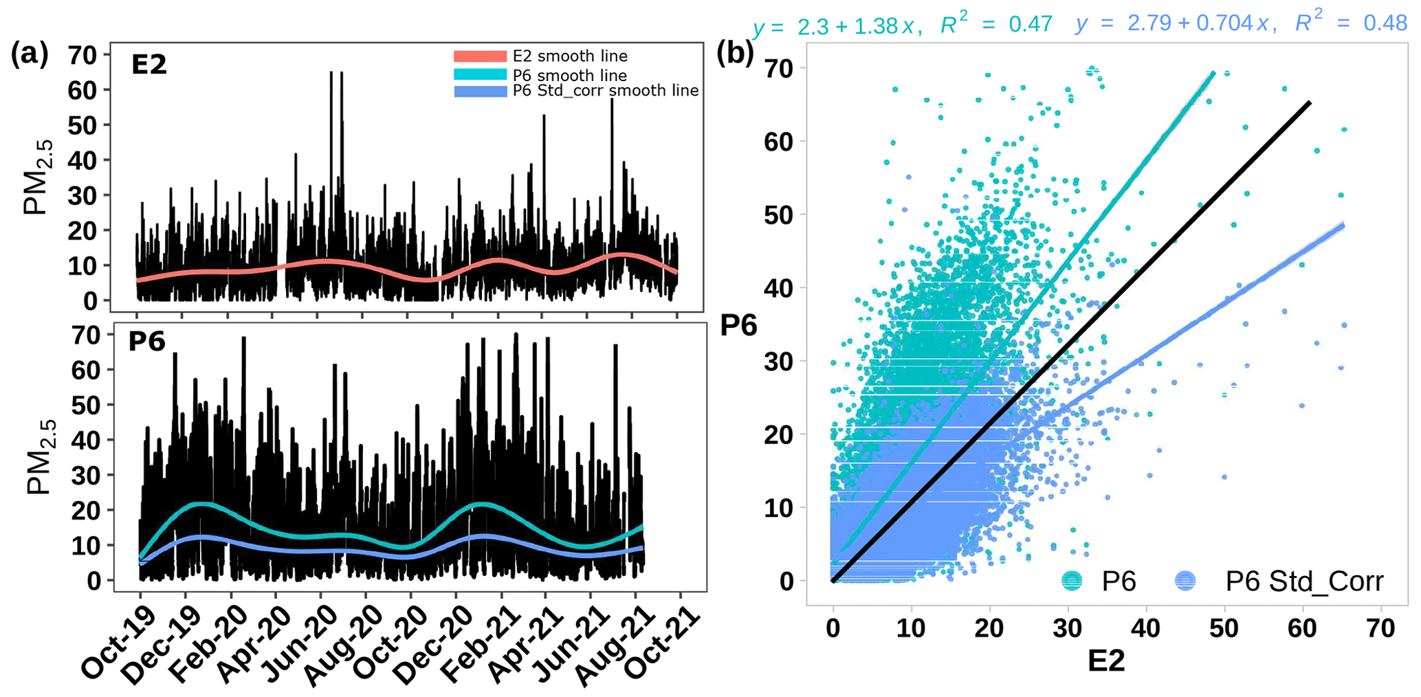
Figure 2 (a) Hourly PM_2.5 measurements from EPA site E2 and PA sensor P6. (b) Hourly PM_2.5 measurements from EPA site E2 vs. PA sensors P6 raw and P6 corrected.

The data from both networks show high temporal variations along with some seasonal trends over longer timescales. A direct comparison of the two data sets (Fig. 2b) for the combination of the E2 and P6 sites shows that, on average, the raw PA data overestimate the EPA data by roughly 40 %, consistent with previous findings. Use of the standard correction results in a decrease in the reported PA values. The resultant best-fit linear model suggests that the corrected data slightly underestimate the actual PM_2.5 by roughly 30 %.

The overall distribution of the PM_2.5 data at each of the EPA and PA sites over the entire time period of our analysis is shown in Fig. 3 and Table S2. The median values of PM_2.5 reported by the PA sites are always higher and more variable than those from the EPA sites in the region. The median PM_2.5 value from the average from the five EPA sites in the region is 8.4 µg m⁻³, while the PA data report a median value of 10 µg m⁻³. With the standard correction it is seen that the variability is reduced and that the median is 6.9 µg m⁻³, 20 % lower than the EPA value.

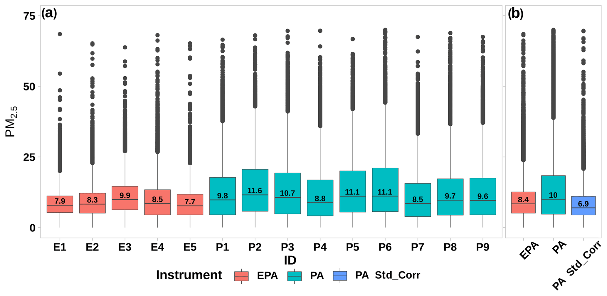
Figure 3 (a) Hourly PM_2.5 measurements from each EPA site and PA sensor located in Cook County, IL. (b) All EPA-, PA-, and PA-corrected data together. The box plots represent the overall distribution with quartile (25th percentile Q₁, median 50th percentile Q₂, and 75th percentile Q₃) values of PM_2.5 data. The values in black dots over Q₃ are outliers.

While the accuracy of the correction model can be improved with some local tuning, it is clear that the model did not improve the quality of the fit. This suggests that the correction model does not account for all of the causes of discrepancy between the two data sets. In particular, a regression-based model will not be able to account for the sensitivity of the sensors to particle compositions and hence to different emission sources. A preliminary validation of model dependence on composition can be obtained from the evaluation of model performance for the prediction of PM_2.5 concentrations during weekdays and weekends. The differing strengths of some emission sources between weekdays and weekends are expected to result in slightly different aerosol populations during these two time periods. Here, we separated the data into weekday and weekend and applied the correction model to get corrected PA data for each of the data sets. A two-sample t test between the EPA and corrected PA data (Fig. 4) shows a statistically significant difference between the two data sets (p value < 0.05 and the exact p value = 0.000007) on weekdays but not on weekends (p value = 0.13), providing some initial validation that the correction model does not account equally for the contributions of all the sources.

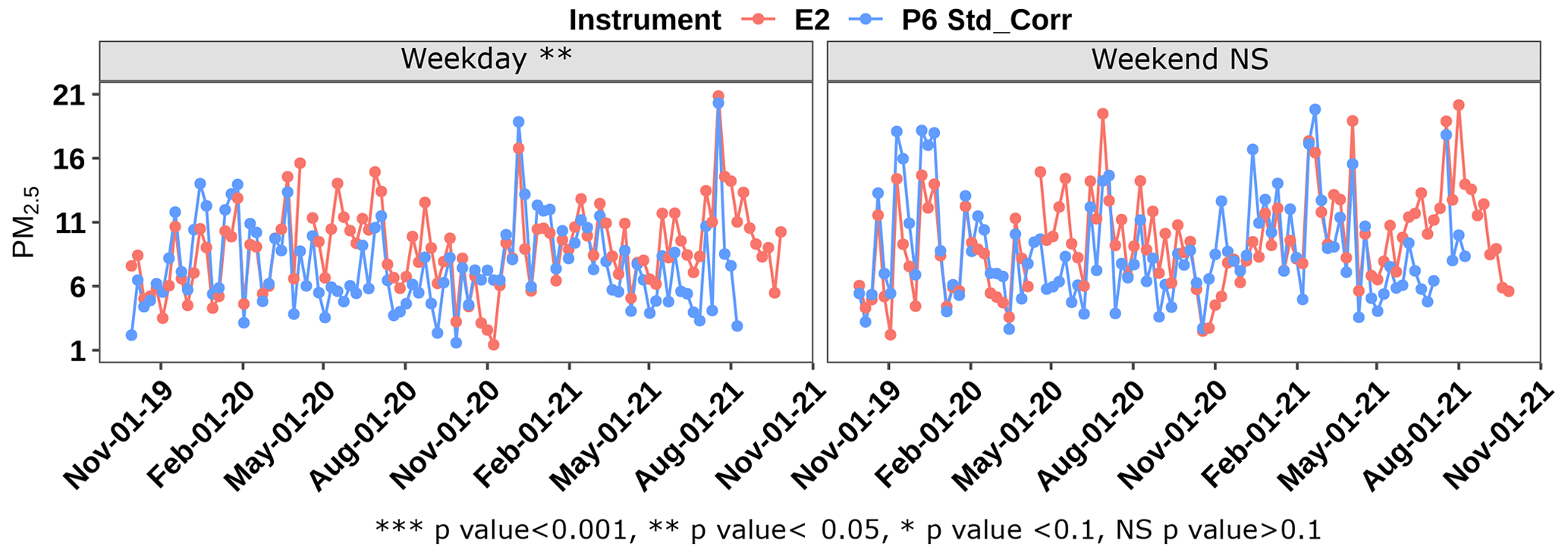
Figure 4 Corrected PA sensor PM_2.5 measurements during weekdays and weekends compared with the nearby EPA sites E2 and P6. The t-test statistics are provided to determine whether there is a statistically significant difference between the two data sets (EPA and PA).

To better understand the causes of model under-performance and to determine the primary drivers of this discrepancy, a frequency-based analysis is helpful. Such an analysis can help extract the contribution of any periodic emission sources that might exist and establish whether the standard correction model provides a bias-free correction for all of these components.

3 Spectral analysis

In meteorology and air quality studies, spectral analysis has been used to extract and examine different temporal components in the obtained data (Hies et al., 2000; Marr and Harley, 2002; Choi et al., 2008; Tchepel and Borrego, 2010). Here, using spectral analysis, we determine the effectiveness of the correction model in improving the correlation of PA data with EPA data over the entire range of emission sources that contribute to Cook County's PM_2.5 population.

To ensure the stationarity of the time series data, i.e., that their statistical properties such as mean, variance, and autocovariance remain constant, we use the augmented Dickey–Fuller (ADF) test method (Wang et al., 2021; Lian and Ma, 2013).

The discrete Fourier transform, X(k), of hourly time series X_t can be calculated using the fast Fourier transform (FFT) algorithm. The power spectral density (PSD) for a finite time series can then be calculated as the squared magnitude of X(k):

$$\begin{array}{}\text{(2)}& \mathrm{\Phi }\left(v_k\right)=\left|X\right(k){|}^{\mathrm{2}}=|{\displaystyle \frac{\mathrm{1}}{\sqrt{N}}}\sum _{t=\mathrm{0}}^{N-\mathrm{1}}{X}_t{e}^{-\mathrm{2}\mathit{\pi }i{v}_{k}t}{|}^{\mathrm{2}},\end{array}$$

where $k=\mathrm{0},\mathrm{1},\mathrm{\dots },(N-\mathrm{1})$. N is the number of observations and $v_k=\frac{k}{N}$.

For a measurement resolution of 1 h, a wave with a period of 2 h or more is required (Nyquist theorem). For spectral analysis using FFT, successive equal-length sequences are required without any missing observations (Dilmaghani, 2007). Here we replace the missing data points from the EPA and PA data sets using the Autoregressive Integrated Moving Average (ARIMA) model with a Kalman filter (Hadeed et al., 2020; Afrifa-Yamoah et al., 2020; Wijesekara and Liyanage, 2020; Saputra et al., 2021). The PSD of each EPA and PA hourly time series of the PM_2.5 data was then calculated using the stats package in R.

3.1 Spectral analysis: results and discussion

We determined the PSD of PM_2.5 data for three data sets – EPA-, PA-, and PA-corrected data – for all of the locations available. Then, the average PSDs for each of the data sets were determined by averaging the individual PSDs of the different locations in each network. By averaging over the different locations, the PSDs in Fig. 5 represent the power spectrum of air quality over the entire Cook County area. The PSD shows that, for both networks (EPA and PA), power is higher in long time periods than in short time periods. Thus, the predominant variation in PM_2.5 data reported by both networks over the studied duration is driven by their long-term trend. The PA data are seen to have lower power compared to the EPA in smaller time periods. Calculating the root mean squared error (RMSE) between the EPA PSD values and the two PA data sets, it is seen that the PSD of the corrected PA data has a 58 % lower RMSE than the uncorrected PA. Thus, applying the US-wide EPA correction model (Eq. 1) to the PA data reduces the PA PSD error relative to the EPA over the entire range of frequencies.

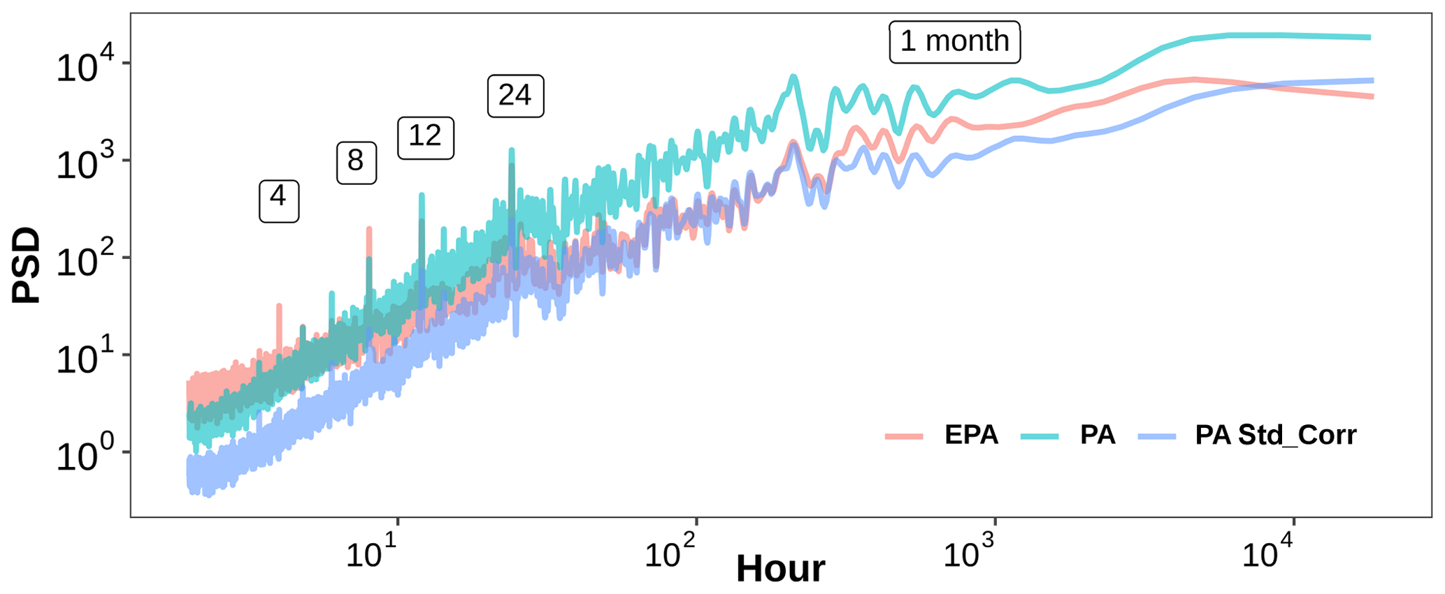
Figure 5 Mean PSD of PM_2.5 data from all the EPA sites, all the PA sensors, and PA standard corrected data.

At small time periods, both networks show distinct peaks at 4, 8, 12, and 24 h, as seen in Fig. 6. These peaks likely represent the contribution of periodic aerosol sources, such as traffic and photochemistry, and diurnal weather patterns to the local air quality. For ease of direct comparison, we removed the baseline trend in each of the data sets, and details about the baseline removal are provided in Sect. S2 in the Supplement. The PSD peak heights at the four time periods are observed to be higher for the EPA data than the PA standard corrected data. The PSD peaks at the four specific time periods were then obtained for each of the five different EPA sites and nine different PA sites and are shown in Fig. 7a. The EPA data peaks are seen to be consistently higher than the PA-corrected data for all four time periods (4, 8, 12, and 24 h) and higher than the PA raw data for all the time periods except 12 h. For the different time periods, the ratio of the median of the PSD peaks of the five EPA sites to the corresponding values for the nine PA sites is shown in Fig. 7b. For the raw PA data, the PSD values for the four time periods, relative to the corresponding EPA values, range from 0.66 to 2.5. After correction, the PA peaks are seen to reduce to below 0.4 for all the time periods, suggesting that the correction model suppresses these peaks.

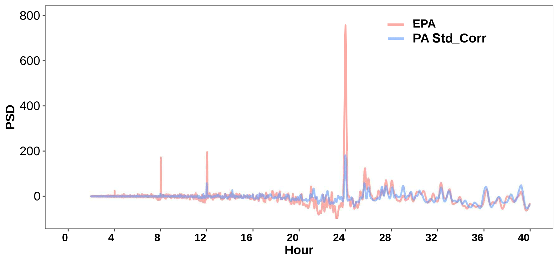
Figure 6 Mean PSD of PM_2.5 data from all the EPA sites, all the PA sensors, and PA standard corrected data at 4 to 40 h peaks of both networks after removing their baselines.

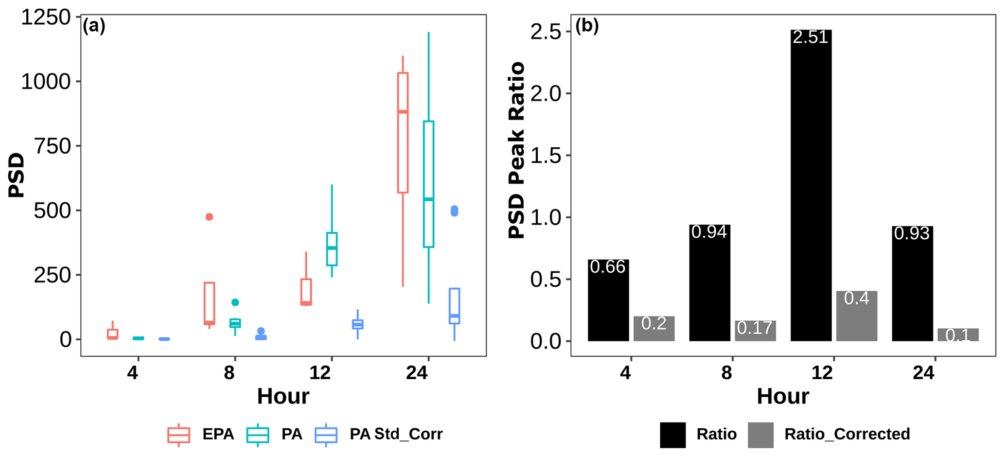
Figure 7 (a) Distribution of PM_2.5 PSD peaks at 4, 8, 12, and 24 h for all the EPA sites and PA locations before and after correction. (b) Ratio of PA to EPA PSD peaks for both raw data (labeled “Ratio”) and corrected data (labeled “Ratio_corrected”).

We speculate that the 4 and 8 h peaks correspond to traffic sources and that the 12 h peak represents the contribution of secondary aerosols formed due to photochemistry and possible diurnal changes in winds and humidity (Jia et al., 2017; Hollaway et al., 2019; Tchepel and Borrego, 2010). The 8 h peak in the raw data is seen to be similar to the EPA data, but the correction results in reducing the peak substantially. The 12 h peak is highly over-represented in the raw data, but the correction model, like for the 8 h peak, decreases the 12 h contribution. The mean sizes of particles formed due to photochemistry are likely larger than the traffic aerosol, resulting in their relatively higher efficiency of detection in low-cost PM sensors (He et al., 2020). The over-correction of the 12 h peak that results in its significant suppression suggests that these particles are likely less hygroscopic than the average particles. The 24 h peak likely represents harmonics of the 8 and 12 h signals and hence represents a combination of both sources.

To confirm that the 8 h peak is traffic-related and that the 12 h peak is likely to be driven by photochemistry, we analyzed changes in these peaks for weekend/weekday and winter/summer. The EPA weekday data were considered to be Monday 00:00 Central Standard Time to Friday 23:59 and weekends to be Saturday 00:00 to Sunday 23:59. The winter data were generated as Dec/Jan/Feb and the summer data as Jun/Jul/Aug. The PSD peaks for the two time periods were then calculated, and the relative changes are shown in Fig. 8. The weekend 8 h PSD peak is seen to be nearly 60 % lower than on weekdays, which is consistent with the changes in traffic patterns expected between the two time periods (Blanchard et al., 2008) and confirms that this peak is indeed traffic-related. Seasonally, the 8 h peak does not change significantly, which again is largely consistent with the expectation that traffic patterns will not be overly dependent on seasons. The 12 h peak also changes on weekends vs. weekdays but has a greater change seasonally than that observed with the 8 h peak. The seasonal change points to the likely contribution of photochemistry to the 12 h peak, but the slight change in this peak between weekends and weekdays also points to contributions from other sources, including possible traffic. In addition, the 4 and 6 h peaks are also likely related to traffic patterns (Sun, 2014).

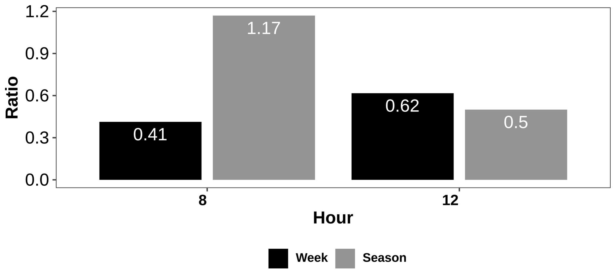
Figure 8 Ratio of EPA PSD peaks at 8 and 12 h for the weekend to weekdays (labeled “week”) and winter to summer (labeled “season”).

From the 8 h PSD peak ratios, it can be concluded that the corrected PA data are significantly under-represented in traffic-related particles, with the PSD value for the corrected PA data being only around 17 % of that of the EPA PSD value for this time period (Fig. 7b). This finding is consistent with general observations in previous studies that low-cost sensor measurements more closely match reference monitors at locations with low traffic than at high-traffic locations (Castell et al., 2017).

4 Local correction model

Some of the imperfections of the correction model could be attributed to the fact that the model was based on data from a wide range of locations with different emission characteristics and meteorology. Consequently, it could be hypothesized that a local correction model tuned to local conditions will result in a better correction of PA data. Additionally, as the standard correction model is built based on daily data, it could be hypothesized that the sub-24 h components may not be accounted for well. To determine whether the sub-24 h components in the PA data could be better matched with EPA data, we built an hourly local correction model using the same approach used in building the standard correction model (Barkjohn et al., 2021). The model was built using PA data from various selected locations and data from the nearest EPA site, with relative humidity and temperature included as predictors. Typically in multiple linear regression (MLR) models, we would only consider independent variables, and it could be argued that temperature and relative humidity are not entirely independent. However, from a particulate matter perspective, the differing impacts of these parameters make them independent of each other. Relative humidity directly affects particle size and hence measurements by low-cost sensors such as PA. Temperature, however, has a more complex connection to particle properties. Temperature directly affects particle size and composition by modulating condensation and evaporation, which can affect PM measurements by both EPA and low-cost sensors. Temperature also indirectly affects PM properties at a location through its relation to local meteorology, especially wind direction, and hence the distribution of sources at the measurement location. To establish the independence of these parameters, we calculated the variance inflation factors (VIFs) for temperature and relative humidity, and these were found to be below 5. These small VIF values indicate a low level of multicollinearity for the two parameters (James et al., 2013) and permit their inclusion in the MLR model. A stepwise forward-selection algorithm was used to build MLR models. A 10-fold cross-validation technique was employed by repeating the process a total of five times. This method of cross-validation involves dividing the data into 10 equally sized folds and training the model on 9 of the folds while using the remaining fold as a hold-out test set. This process is repeated 10 times, with each fold serving as the test set once. By repeating the process five times, the robustness of the developed model is increased by training and testing it on different subsets of the data.

The obtained equation for the local correction model is

$$\begin{array}{}\text{(3)}& \begin{array}{rl}{\mathrm{PM}}_{\mathrm{2.5}}\mathrm{Loc}\mathit{\_}\mathrm{Corr}& =\mathrm{0.44}{\text{PA}}_{\mathrm{cf}\mathit{\_}\mathrm{1}}{\mathrm{PM}}_{\mathrm{2.5}}-\mathrm{0.026}\text{RH}\\ & +\mathrm{0.023}\text{temperature}+\mathrm{19.76},\end{array}\end{array}$$

where PA_{cf_1} represents the PA data with the higher correction factor cf_1 reported at a specific sensor, and RH and temperature are obtained from the PA network.

After obtaining the model, its performance was evaluated using several metrics: R², RMSE, and mean absolute error (MAE) (see the Supplement for details about these metrics). The model performances of the standard correction and local correction models are summarized in Table S3. The effectiveness of the local correction model in improving the accuracy of the PA data and addressing the problem of under-accounting of high-frequency sources such as traffic must be ascertained.

5 Time series decomposition

For a full model evaluation, its performance will be determined for three time period components: less than 12 h (short term), 12 h to a month (medium term), and more than a month (long term). The short-term component represents the changes in PM_2.5 data due to high-frequency sources such as traffic and short-term weather events. The medium-term component accounts for variations within time periods between 12 h and a month. The long-term component primarily captures low-frequency emissions such as those related to seasonal changes in weather and meteorology and changes in emission rates over time (Rao and Zurbenko, 1994; Rao et al., 1997; Wise and Comrie, 2005).

To separate the time series data into the three components of short-term, medium-term, and long-term time periods, we use the Kolmogorov–Zurbenko (KZ) filter technique (Rao and Zurbenko, 1994), as was done in several recent PM_2.5 studies (Bai et al., 2022; Fang et al., 2022; Zhang et al., 2018; Sá et al., 2015). The KZ filter is a low-pass filter produced through repeated iterations of the moving average with the parameters moving window (m) and iterations (p), also known as KZ_m,p:

$$\begin{array}{}\text{(4)}& Y_t={\displaystyle \frac{\mathrm{1}}{m}}\sum _{j=-k}^k{X}_{t+j},\end{array}$$

where Y_t is a filtered time sequence, X_t is the input time series, k is the number of values included on each side of the targeted value, $m=\mathrm{2}k+\mathrm{1}$ is the window length, t is the time index, and j is the time point of sliding.

The output of the first pass then becomes the input for the next pass. Adjusting the window length and the number of iterations makes it possible to control the filtering of different scales of motion (Eskridge et al., 1997; Milanchus et al., 1998). To filter a period of fewer than N days, the following criterion is applied to determine the filter's effective width (Wise and Comrie, 2005):

$$\begin{array}{}\text{(5)}& m\times p^{\mathrm{1}/\mathrm{2}}\le N.\end{array}$$

Also, the filter can be used to remove frequencies below a desired cutoff frequency w₀ (Rao et al., 1997):

$$\begin{array}{}\text{(6)}& w_{\mathrm{0}}\approx {\displaystyle \frac{\sqrt{\mathrm{6}}}{\mathit{\pi }}}\sqrt{{\displaystyle \frac{\mathrm{1}-(\mathrm{1}/\mathrm{2}{)}^{\mathrm{1}/\mathrm{2}p}}{m^{\mathrm{2}}-(\mathrm{1}/\mathrm{2}{)}^{\mathrm{1}/\mathrm{2}p}}}}.\end{array}$$

The cutoff period can be obtained by $\frac{\mathrm{1}}{w_{\mathrm{0}}}$. For our study, we have used the following equations to get long-term, medium-term, and short-term components of the time series of PM_2.5 data as defined by Hogrefe et al. (2000) and Kang et al. (2008).

The long-term PM_2.5 (PM_2.5,B) component is obtained as

$$\begin{array}{}\text{(7)}& {\mathrm{PM}}_{\mathrm{2.5},B}\left(t\right)={\mathrm{KZ}}_{\mathrm{900},\mathrm{5}}{\mathrm{PM}}_{\mathrm{2.5}}\left(t\right).\end{array}$$

The medium-term PM_2.5 (PM_2.5,M) component is obtained as

$$\begin{array}{}\text{(8)}& {\mathrm{PM}}_{\mathrm{2.5},M}\left(t\right)={\mathrm{KZ}}_{\mathrm{3},\mathrm{3}}{\mathrm{PM}}_{\mathrm{2.5}}\left(t\right)-{\mathrm{KZ}}_{\mathrm{13},\mathrm{5}}{\mathrm{PM}}_{\mathrm{2.5}}\left(t\right).\end{array}$$

The short-term PM_2.5 (PM_2.5,S) component is obtained as

$$\begin{array}{}\text{(9)}& {\mathrm{PM}}_{\mathrm{2.5},S}\left(t\right)={\mathrm{PM}}_{\mathrm{2.5}}\left(t\right)-{\mathrm{KZ}}_{\mathrm{3},\mathrm{3}}{\mathrm{PM}}_{\mathrm{2.5}}\left(t\right).\end{array}$$

5.1 Time series decomposition: results and discussion

We separated the time series of PM_2.5 data from EPA, PA, and standard and local corrected PA data (Eqs. 7–9) into the three time periods of long term, medium term, and short term in Fig. 9. A comparison of the long-term component signals shows that the 2-year trends of the PA raw data are different from those of the EPA data (Fig. 9a). Both correction models lower the mean of the PA data. The standard correction is, however, seen to over-correct for the mean and does not capture the signal density accurately. Using the local model results in largely replicating the long-term PM_2.5 distribution, except at the lowest values. This might suggest that long-term changes might be driven by more than humidity, and including the effect of temperature on sensor performance could be important. In addition to air properties, long-term changes may also be driven by a drift in sensor performance, which could be captured with a local model but not with a standard model. In the medium term, the standard correction model shifts the mean PM_2.5 values, in contrast to the long-term component, to align reasonably with the EPA data, as illustrated by the density plot in Fig. 9b. The performance of the local correction model is seen to match the standard correction model, suggesting that, over this medium term, relative humidity is probably the primary driver of aerosol changes. In the short term, the density plot shows that both the standard and local correction models fail to capture the PM_2.5 distribution accurately. In fact, the use of the correction models then dampens any contribution of short-term sources to the total signal and increases the difference between the EPA and PA data sets (Fig. 9c). This suggests that the primary drivers of short-term fluctuations are particles that are poorly sensed by the PA sensors, and regression-based correction models, including both the standard correction model and the local correction model, cannot capture the contributions of those particles.

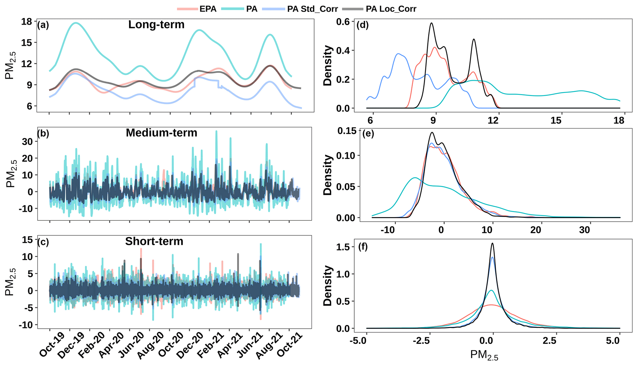
Figure 9 Time series and density plot of EPA data, PA data, corrected PA data using the standard correction model, and corrected PA data using a local correction model for a (a) long-term component, (b) medium-term component, and (c) short-term component.

6 Applicability of the method

Air monitoring data, such as PM_2.5, exhibit source dependence. Data from low-cost sensors with high spatiotemporal resolution require careful analysis. This method provides a framework where, instead of solely relying on time series data comparison, frequency-based or spectral analysis can be incorporated to identify periodicities in the data. It also offers a means to assess the accuracy of models through not just performance metrics like RMSE, but also by incorporating PSD and time series decomposition to evaluate data accuracy in short-, medium-, and long-term components. Based on long-, medium-, and short-term component assessment, further improvements can be made to sensor technology and the correction models. This method is applicable to air pollution and weather data sets where periodic patterns and source dependencies are evident.

7 Study limitations

This study has a few limitations. Firstly, the study is limited to one city, and the low-cost air quality sensor network used in the study is not perfectly co-located with the EPA monitoring sites. This can introduce uncertainties in the analysis due to differences in local air properties and pollution sources for the two data sets. Secondly, the placement of the low-cost sensors relative to locally built structures could affect its measurement performance and increase data uncertainty, but this information is not available to us. Thirdly, we did not have access to local traffic-related information or industrial activity, restricting our ability to strongly relate frequency components to specific emission sources. The likely variability of the local emission sources at the different PurpleAir and EPA sites adds uncertainty in quantifying the differences in the short-term responses of the two networks.

8 Conclusions

The use of low-cost sensors for air quality monitoring is becoming more widespread, and their use has resulted in a better understanding of air quality at a hyper-local level. Several studies have shown that data from low-cost sensors such as from the PurpleAir (PA) network are less accurate than the gold-standard EPA data. Other studies have reported that, using correction models, PA data can become comparable to EPA data in accuracy (Mei et al., 2020; Ardon-Dryer et al., 2020; Barkjohn et al., 2021). Understanding the quality of the data reported by low-cost air sensor networks is critical to determining the extent and limitations of the use of these data in policy-making and health studies.

Here, using long-term PM_2.5 measurements from the EPA and PA networks in the Cook County, IL, area, we evaluated the accuracy of the reported raw data and recommended correction models. Our initial analysis showed that the corrected PA data were, on average, under-predicting PM_2.5 by 30 % in the study area. To determine the cause of the discrepancy between the PA and EPA data sets, we used a spectral analysis approach to identify the presence of periodic sources, i.e., at 4, 8, 12, and 24 h in both data sets, and then determined their relative responses to these sources. Our analysis clearly demonstrates the PA network's very different sensitivity to different sources. The use of the standard correction model, i.e., the US-wide correction model discussed in Eq. (1), results in correction of the PA data but significant under-presentation of high-frequency sources, particularly traffic. The reason why low-cost sensors may be missing high-frequency components from sources such as traffic can be attributed to several factors. One factor is the minimum detection size limit of the sensors, which is ∼ 300 nm. Sources such as traffic with PM emissions predominantly in the sub-300 nm size range will, thus, be under-detected in low-cost sensors. EPA measurements do not have this limitation. Additionally, the low-cost sensor response depends on the composition and shape of particles, resulting in PM measurement accuracy varying with emission sources. The implication of these limitations is that the measurements provided by low-cost sensors, such as those in PurpleAir, will be underestimated with respect to certain pollutants, including those associated with traffic emissions, and overestimated relative to others. Consequently, relying solely on low-cost sensor measurements without considering the limitations in particle detection and composition could result in an incomplete understanding of air quality, especially in relation to specific pollutant sources or components.

Also, the standard correction model over-corrects for some sources, such as the 12 h time period source that we identified in this study. Using a local correction model based on temperature and relative humidity, we showed that the long-term and medium-term trends in PA data can be matched with EPA data. In the short term, both the local and standard correction models perform poorly. The use of both these models actually results in suppression of the contribution of high-frequency sources. Also note that, while this study identified several significant peaks, i.e., 4, 8, 12, and 24 h, in the power spectrum analysis of air quality data, their precise sources require further analysis and validation.

Our study also demonstrates that, while regression-based correction models may seem to improve the accuracy of low-cost sensor network performance by accounting for the contribution of meteorology, they do not uniformly improve the network response to all emission sources. Any field calibration of these sensors using simple regression models cannot correct for this non-uniform contribution. As best practice, it is recommended that calibration models from field data should report, at a minimum, the distribution of different PM emission sources at that location and ideally also the particle size distributions. Given the periodic signatures of many sources, a frequency-based scaling approach should be explored towards the development of more robust calibration models that account for the wide range of emission sources common in urban environments. The accuracy of such models will scale with time periods of calibration. Considering the source-dependent response of low-cost sensors, calibration models developed using land use data might be an advance over simple regression models.

Thus, care must be taken in using their data in studies where a diversity of emission sources may be present and their relative strengths are varying over time or space. Advances in sensing technologies and improvements in correction models are critical for expanding our use of data from these emerging low-cost sensor networks.