the Creative Commons Attribution 4.0 License.
the Creative Commons Attribution 4.0 License.
 | 30 Jan 2023
Estimates of the spatially complete, observational-data-driven planetary boundary layer height over the contiguous United States
Zolal Ayazpour
Shiqi Tao
Amy Jo Scarino
Ralph E. Kuehn
This study aims to generate a spatially complete planetary boundary layer height (PBLH) product over the contiguous United States (CONUS). An eXtreme Gradient Boosting (XGB) regression model was developed using selected meteorological and geographical data fields as explanatory variables to fit the PBLH values derived from Aircraft Meteorological DAta Relay (AMDAR) reports hourly profiles at 13:00–14:00 LST (local solar time) during 2005–2019. A preprocessing step was implemented to exclude AMDAR data points that were unexplainable by the predictors, mostly under stable conditions. The PBLH prediction by this work as well as PBLHs from three reanalysis datasets (the fifth-generation European Centre for Medium-Range Weather Forecasts atmospheric reanalysis of the global climate – ERA5; the Modern-Era Retrospective analysis for Research and Applications, Version 2 – MERRA-2; and the North American Regional Reanalysis – NARR) were compared to reference PBLH observations from spaceborne lidar (Cloud-Aerosol Lidar and Infrared Pathfinder Satellite Observations, CALIPSO), airborne lidar (High Spectral Resolution Lidar, HSRL), and in situ research aircraft profiles from the Deriving Information on Surface Conditions from Column and Vertically Resolved Observations Relevant to Air Quality (DISCOVER-AQ) campaigns. Compared with PBLHs from reanalysis products, the PBLH prediction from this work shows closer agreement with the reference observations, with the caveat that different PBLH products and estimates have different ways of identifying the PBLH; thus, their comparisons should be interpreted with caution. The reanalysis products show significant high biases in the western CONUS relative to the reference observations. One direct application of the dataset generated by this work is that it enables sampling of the PBLH at the sounding locations and times of sensors aboard satellites with an overpass time in the early afternoon, e.g., the Afternoon Train (A-train), the Suomi National Polar-orbiting Partnership (Suomi NPP), the Joint Polar Satellite System (JPSS), and the Sentinel-5 Precursor (Sentinel-5P) satellite sensors. As both AMDAR and ERA5 are continuous at hourly resolution, the observational-data-driven PBLHs may be extended to other daytime hours.
- Article
(6685 KB) - Full-text XML
- BibTeX
- EndNote


The planetary boundary layer (PBL) is the lowest part of the atmosphere that mediates the exchange of momentum, energy, and mass between the surface and the overlying free troposphere (Stull, 1988). It plays a central role in land–atmosphere coupling, linking surface states and characteristics (e.g., surface temperature, soil moisture, and vegetation) to convection through surface fluxes of sensible and latent heat (Santanello et al., 2018). Improving our understanding and characterization of the PBL is critical for enhancing the predictability of numerical weather prediction and global climate and Earth system models (Garratt, 1994; Stensrud, 2009). The PBL height (PBLH), which characterizes the vertical extent of the PBL, is a critical parameter in many land–atmosphere coupling metrics (Santanello et al., 2013, 2015). The PBLH also governs the vertical mixing of thermal energy, water, and trace gases and, hence, strongly regulates the near-surface pollutant concentrations. With the same amount of emission, a higher PBLH typically means stronger dilution and, hence, lower near-surface concentrations (and vice versa for a lower PBLH). Therefore, accurate knowledge of the PBLH is important in the modeling of air quality through a chemical transport model (Zhu et al., 2016) and in the inference of emissions through inverse methods (Gerbig et al., 2008). The PBLH can also help bridge the gaps between the column-integrated quantities observed by satellites and near-surface concentrations for short-lived species such as fine aerosols (Su et al., 2018), NO2 (Boersma et al., 2009), and NH3 (Sun et al., 2015). In order to sample the PBLH values at the satellite sounding locations and times (Sun et al., 2018), extensive spatiotemporal coverage of the PBLH data is needed.
Spatially and temporally complete estimates of the PBLH can be provided by atmospheric models or reanalysis products, although the PBLH is generally not directly simulated but rather diagnosed from model profiles of wind, temperature, or turbulent kinetic energy (TKE). Besides the inherent modeling uncertainties, PBLH estimation methods and the associated empirical parameters in these methods introduce additional uncertainties and inconsistency among models. The PBLH products from three commonly used reanalysis products are evaluated in this work: the fifth-generation European Centre for Medium-Range Weather Forecasts (ECMWF) atmospheric reanalysis of the global climate (ERA5) (Hersbach et al., 2020); Modern-Era Retrospective analysis for Research and Applications, Version 2 (MERRA-2) from NASA (Gelaro et al., 2017); and the North American Regional Reanalysis (NARR) from NOAA National Centers for Environmental Prediction (NCEP) (Mesinger et al., 2006). The PBLH values were determined by different methods in these three reanalysis products: critical bulk Richardson number for ERA5, threshold total eddy diffusion coefficient of heat for MERRA-2, and threshold TKE value for NARR. Validations of those model-based PBLH products by observations are limited, and discrepancies are frequently observed (Zhang et al., 2020). The PBLHs from MERRA-2 and NARR are widely used in the GEOS-Chem and WRF-Chem chemical transport models, respectively (Lu et al., 2021; Murray et al., 2021; Laughner et al., 2019; Hegarty et al., 2018). If the PBLHs from those reanalysis models were biased, the associated chemical transport model simulations would be directly impacted. McGrath-Spangler and Denning (2012) found that the PBLH in MERRA (the previous version of MERRA-2) was higher than the retrieved PBLH from the CALIOP (Cloud-Aerosol Lidar with Orthogonal Polarization) spaceborne lidar aboard the Cloud-Aerosol Lidar and Infrared Pathfinder Satellite Observation (CALIPSO) satellite over the arid and semiarid regions of North America, where NARR gave even higher PBLH values than MERRA. Comparisons between the PBLH from GEOS-FP (forward processing), the assimilated meteorological fields generated by the same model used for MERRA-2 (i.e., the Goddard Earth Observing System, Version 5, GEOS-5 model), and lidar/ceilometer data showed a 30 %–50 % high bias in the southeastern US (Zhu et al., 2016; Millet et al., 2015). Zhang et al. (2020) compared the ERA5 PBLHs with those derived from hourly profiles measured by commercial airlines in the Aircraft Meteorological DAta Relay (AMDAR) reports (Zhang et al., 2019) and found that ERA5 overestimates the daytime PBLH over the contiguous United States (CONUS) by 18 %–41 %. Furthermore, models and reanalysis products often disagree with continuous observations in terms of the diurnal evolution of the PBLH (Zhang et al., 2020; Hegarty et al., 2018).
In spite of its importance, observations of the PBLH are sparse in both space and time. Operational radiosondes launched twice daily at 00:00 and 12:00 UTC have been used to construct long-term PBLH climatology (Guo et al., 2016; Seidel et al., 2012), but the launching times largely missed the daytime variations in the PBLH over the CONUS (Zhang et al., 2020). On the other hand, intensive in situ atmospheric profiling by radiosondes or aircraft spiraling profiles (e.g., the NASA Deriving Information on Surface Conditions from Column and Vertically Resolved Observations Relevant to Air Quality, or DISCOVER-AQ, campaign) are limited to short periods and certain locations (Angevine et al., 2012; Zhang et al., 2016). In addition to radiosondes and aircraft spiraling profiles, ground-based, airborne, and spaceborne lidar remote sensing of aerosol backscatter also provide PBLH observations. For example, Hegarty et al. (2018) synergized a network of ground-based micropulse lidar (MPL), an airborne High Spectral Resolution Lidar (HSRL), and the CALIPSO spaceborne lidar to examine the diurnal PBLH variations during the DISCOVER-AQ campaign in the Maryland–Washington, D.C. area. Compared with surface and suborbital lidar observations, CALIPSO provides better spatial (global coverage) and temporal (from 2006 to present) coverage. However, there is no official CALIPSO PBLH product available, and existing PBLH retrievals from CALIPSO Level 1B data have low temporal resolution because the CALIPSO ground track is sparse with a 16 d repeat cycle (Jordan et al., 2010; McGrath-Spangler and Denning, 2012, 2013; Su et al., 2018). The other PBLH observation data source is AMDAR which provides global automated weather reports from commercial aircraft (Moninger et al., 2003). Zhang et al. (2020) derived the PBLH from AMDAR profiles and constructed a continuous hourly climatology of the PBLH at 54 major airports in the CONUS. The same methodology developed by Zhang et al. (2020) can be readily applied to other regions in the world where major commercial airports exist and to other time periods given the operational status of AMDAR observations. Compared with the existing CALIPSO PBLH product, the hourly PBLH derived from AMDAR profiles features a more complete temporal coverage and higher signal-to-noise ratios. Therefore, the AMDAR PBLH dataset is selected as the observational PBLH data source for this research.
The existing AMDAR PBLH dataset is available at an hourly resolution from 2005 to 2019 at 54 airport locations. However, many applications require the PBLH at other locations or complete coverage of a region. The objective of this study is to produce observation-based, spatially complete PBLH fields over the CONUS. We develop a data-driven predictive model using various meteorological and geographical predictors to match the AMDAR PBLH observations. As the predictors all have complete spatial coverage over the CONUS, running the model in the forward direction can yield PBLH prediction at arbitrary locations in the domain. We cross-validate the model in space by randomly splitting the airports into training and testing sets, and the model is selected based on averaged metrics from the testing sets. The predicted PBLH is then compared to PBLHs from three widely used reanalysis products (ERA5, MERRA-2, and NARR), and all of them are further compared to the independently diagnosed PBLH from observations (e.g., from research aircraft profiles and HSRL airborne lidar) and the CALIPSO PBLH product. Here, we should emphasize that such comparisons should be interpreted with caution because different PBLH products and estimates have different ways of identifying the PBLH. In this sense, none of the PBLH products and estimates should be treated as the golden truth. However, such comparisons remain meaningful because (1) they provide confidence in the PBLH prediction by this work and (2) they generate information regarding the difference between various PBLH products and estimates that have been widely used in previous work.
One direct application of the PBLH product from this work is that it enables sampling of the PBLH at the sounding locations and times of satellite sensors with an overpass time in the early afternoon, e.g., the Afternoon Train (A-train) sensors as well as sensors aboard similar polar-orbiting platforms, such as the Cross-track Infrared Sounder (CrIS) and TROPOspheric Monitoring Instrument (TROPOMI). As both AMDAR and ERA5 are continuous at an hourly resolution, future work may extend to other daytime hours observable by geostationary missions like TEMPO (Tropospheric Emissions: Monitoring of Pollution based on Zoogman et al., 2017) and potentially to existing satellites with drifted orbits such as the NASA Earth Observing System (EOS) satellites.
The training data used to estimate the spatially complete PBLH over the CONUS were obtained from AMDAR observations. The relevant meteorological data from ERA5 as well as geographical data were used as explanatory variables, i.e., predictors or features, in a data-driven predictive model to predict PBLH at AMDAR observation locations. The model prediction at locations other than AMDAR observation locations was evaluated using three independent observational datasets: (1) the Surface Attached Aerosol Layer product from CALIPSO, (2) NASA HSRL observations during the DISCOVER-AQ campaigns and the Studies of Emissions, Atmospheric Composition, Clouds and Climate Coupling by Regional Surveys (SEAC4RS) campaign, and (3) the manually labeled PBLH from spiraling profiles during DISCOVER-AQ. In this study, we only focus on data from 13:00 to 14:00 LST (local solar time). In addition to the validation with ground measurements, we also compared our estimations with PBLH data from ERA5, MERRA-2, and NARR. Detailed descriptions of these datasets are provided in the following.
2.1 The AMDAR observations
AMDAR provides meteorological data captured by sensors aboard commercial aircraft worldwide. In this study, we used all quality-assured data from 54 airports within the CONUS from 2005 to 2019. The locations of these airports are shown in Fig. 1a. Vertical profiles of potential temperature, humidity, and wind speed were averaged over each UTC hour at each airport (Zhang et al., 2019). The PBLH was derived using the bulk Richardson number method (Seidel et al., 2012; Zhang et al., 2020), where the bulk Richardson number is calculated as
Here, g is gravity acceleration, θv is virtual potential temperature, u and v are horizontal winds, and u* is the surface friction velocity. Subscript z denotes vertical profile values, and subscript s denotes values at the lower boundary of the PBL. We use zs=40 m, b=100, and a critical bulk Richardson number of 0.5, following Zhang et al. (2020). Regarding u*, Zhang et al. (2020) tested two options, one using u* from ERA5 and the other one using a constant m s−1, and found that the results were similar. We choose the latter option so that the AMDAR PBLH is purely observation-based and independent of the reanalysis.
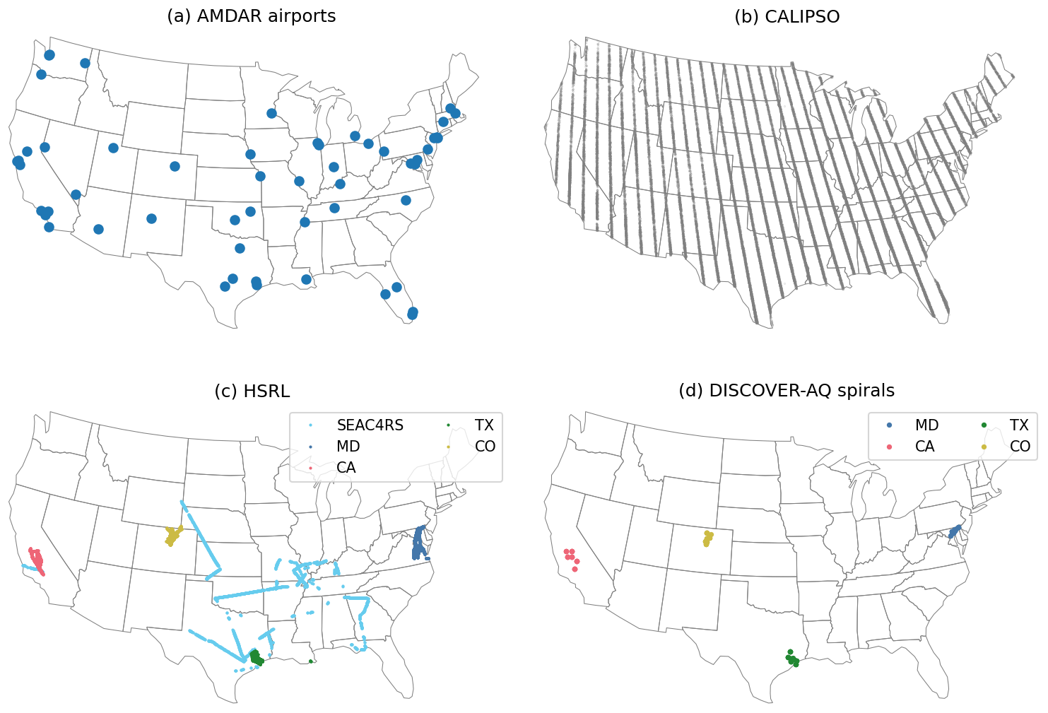
Figure 1Overview of the locations of the main source of the AMDAR PBLH observation dataset (a) and the three independent validation datasets from the CALIPSO spaceborne lidar (b), the HSRL airborne lidar (c), and in situ aircraft spiral profiling during the DISCOVER-AQ campaigns (d). The HSRL and spiral-profile data were limited to 12:30–14:30 LST only, and the CALIPSO overpasses were always at around 13:30 LST.
Although the bulk Richardson number method was found to be the most robust one to derive the PBLH from AMDAR-measured profiles, significant challenges remain under stable conditions. Figure 2a–c compare all AMDAR-derived PBLHs at 13:00–14:00 LST with spatiotemporally interpolated PBLHs from ERA5. Under stable and, to a lesser extent, neutral conditions, a significant portion of data cluster close to the horizontal axis (Fig. 2a, b), indicating that AMDAR gives very low PBLHs (<500 m), whereas ERA5 reports a wide range of PBLH values up to 3000 m. We did not find any meteorological or geographical factors that would explain the occurrence of AMDAR vs. ERA5 PBLH data pairs in these clusters. The most likely cause of these clusters of data is the ambiguity of identifying the PBL top. Under challenging conditions, the critical bulk Richardson number algorithm that is used in AMDAR and ERA5 data to diagnose the PBLH may identify different vertical structures as the PBL top, leading to very different and uncorrelated PBLH values. Including these uncorrelated clusters of points will strongly bias the model training results. Consequently, we use quantile regression (Hirschi et al., 2011) to filter them out in order to avoid significant bias in the model training.
Quantile regression fits a series of regression lines that correspond to different quantiles of the AMDAR PBLH distribution conditioned on the ERA5 PBLH values. The distribution of slopes from 0 to 100 quantile lines is displayed in Fig. 2d. The overall slopes are smaller than unity, indicating that the AMDAR PBLH is generally lower than ERA5. The slopes show a bimodal distribution due to the two clusters of AMDAR–ERA5 relationship. We choose a slope threshold of 0.5 (highlighted in Fig. 2d) to separate the data cluster near the 1:1 line and the data cluster near the horizontal axis. The quantile regression line corresponding to a slope of 0.5 is labeled and plotted in Fig. 2a–c. All data points below this line were removed from further analysis, which accounted for about one-third of all AMDAR data, half of the data under stable conditions, and only 10 % of data under convective conditions. The distribution of the AMDAR PBLH after such a filtering is shown in Fig. 3a.
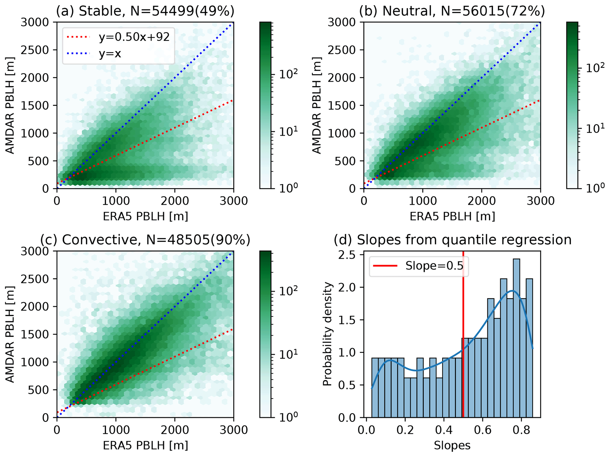
Figure 2Comparison between PBLHs from AMDAR and ERA5 under stable (a), neutral (b), and convective (c) conditions, where atmospheric stability is classified using AMDAR profiles following Zhang et al. (2020). The blue and red dashed lines are the 1:1 line and the quantile regression line corresponding to a slope of 0.5, respectively. The titles give the total number of points as well as the percentage of data points above the 0.5-slope line, i.e., the fraction of data after filtering. Panel (d) shows the distribution of quantile regression slopes, where 0.5 marks the threshold between two clusters.
2.2 Reanalysis datasets
2.2.1 ERA5
ERA5 provides multiple climate variables at a spatial resolution of 0.25 degree (approximately 30 km) for the globe every hour, with 137 levels from the surface up to 0.01 hPa (around 80 km height). Currently ERA5 extends from 1970 to 5 d earlier than the present date. Hourly single-level ERA5 fields (ECMWF, 2020) were obtained from the Copernicus Climate Data Store (https://cds.climate.copernicus.eu/, last access: 15 July 2022) and spatiotemporally sampled at the coordinate and time of AMDAR observations as explanatory variables for model construction. The ERA5 PBLH was also spatiotemporally sampled at the independent observation coordinate and time for intercomparison. The PBLH from the ERA5 product is identified using the bulk Richardson number method but with slightly different parameters (ECMWF, 2017). Zhang et al. (2020) compared the AMDAR PBLH estimated with the same parameters as ERA5, but the results gave larger biases relative to ERA5 and other observations.
2.2.2 MERRA-2
Extending from 1980 to around 1 month earlier than the present date, MERRA-2 is the first long-term global reanalysis dataset that assimilates observational records of aerosol and its impact on other physical processes. MERRA-2 is widely used as meteorological fields for the GEOS-Chem chemical transport model (Hu et al., 2017; Lu et al., 2021; Murray et al., 2021). The spatial resolution of MERRA-2 is 0.5∘ × 0.625∘. The PBL top pressure in MERRA-2 is identified as the model level under which the total eddy diffusion coefficient of heat falls below the threshold value of 2 m2 s−1 (McGrath-Spangler and Molod, 2014). We obtained hourly PBL top pressure and surface pressure fields from the MERRA-2 time-averaged single-level diagnostics collection (GMAO, 2015) and calculated the PBLH using a scale height of 7500 m. The MERRA-2 PBLH was then spatiotemporally sampled at the independent observation coordinate and time for intercomparison.
2.2.3 NARR
The NARR reanalysis covers North America with a 3 h temporal resolution and a 32 km spatial resolution. It is commonly used as initial and boundary conditions to drive WRF and WRF-Chem simulations for atmospheric composition studies (e.g., Laughner et al., 2019; McKain et al., 2012; Hegarty et al., 2018). The NARR PBLH is computed from the TKE profile which is calculated with a Level-2.5 Mellor–Yamada closure scheme (Lee and De Wekker, 2016). We obtained the NARR PBLH field from the National Center for Atmospheric Research (NCAR) Research Data Archive (NCEP, 2005) and sampled it at the observational coordinate/time for intercomparison.
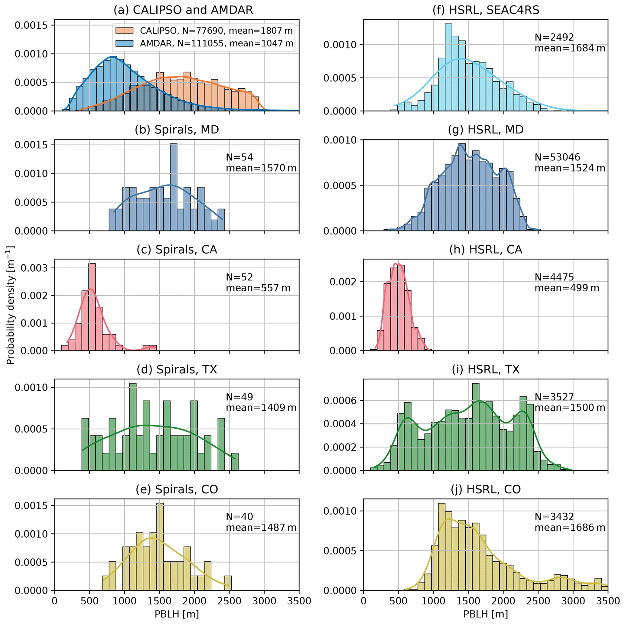
Figure 3(a) Distributions of the AMDAR PBLH after quantile-regression-based filtering and the CALIPSO PBLH over the CONUS. (b–e) Distributions of the PBLH manually labeled using spiral profiles during the DISCOVER-AQ campaigns. (f–j) Distributions of the PBLH from HSRL during the SEAC4RS and DISCOVER-AQ campaigns. The airborne campaign data were limited to 12:30–14:30 LST. The bins denote the normalized histograms, and the lines denote smoothed kernel density estimations. The total number of PBLH data points and the mean values are included in each panel.
2.3 Observational datasets used for evaluation
2.3.1 CALIPSO
The CALIPSO satellite was launched into the A-train in 2006 and carries the CALIOP instrument, a two-wavelength (532 and 1064 nm) polarization-sensitive lidar. The CALIPSO observation is only available at nadir and at around 13:30 LST with a 16 d repeat cycle. A wavelet covariance transform analysis technique similar to that used in Davis et al. (2000) was applied to identify the surface-attached aerosol layer height as a proxy for the PBLH. The algorithm has been improved to work with the lower signal-to-noise ratio (SNR) data provided by CALIPSO and has also been automated to generate global data without intervention. The retrieval methodology was previously validated through comparison with Tropospheric Airborne Meteorological Data Reporting (TAMDAR) observations and HSRL observations from aircraft platforms. We obtained the CALIPSO data from 2006 to 2013 from the University of Wisconsin–Madison Space Science and Engineering Center website (https://download.ssec.wisc.edu/files/calipso/, last access: 15 July 2022). The spatial distribution of CALIPSO sampling locations is shown in Fig. 1b. During the evaluation, we first obtained the model prediction at the same location and time of each CALIPSO sounding and then compared the predicted PBLH with the CALIPSO PBLH. The CALIPSO data provide much more uniform spatial and temporal coverage than the other validation datasets from airborne campaigns, which are only available in limited spatiotemporal ranges. One should note that the backscatter measurements from airborne and spaceborne lidar characterize the mixed layer or surface-attached aerosol layer height, which may be deeper than the PBLH derived based on temperature profiles. In this study, we consider all of these as different estimates of the PBLH. The distribution of all CALIPSO PBLHs is also plotted in Fig. 3a. The CALIPSO PBLH distribution (mean value of 1807 m) is significantly shifted to higher values relative to the distribution of the AMDAR PBLH (mean value of 1047 m), with the caveat that the distributions of CALIPSO and AMDAR are not directly comparable given their different sampling methods and the large uncertainty from CALIPSO.
2.3.2 The NASA HSRL observations
We compiled NASA Langley Research Center airborne HSRL observations from DISCOVER-AQ campaigns in the Maryland–Washington, D.C. area (simplified as MD, July 2011), California (CA, January–February 2013), Texas (TX, September 2013), and Colorado (CO, July–August 2014) and the SEAC4RS campaign (carried out using the differential absorption lidar/High Spectral Resolution Lidar, DIAL/HSRL, instrument) over the southeastern US in August–September 2013. A Haar wavelet algorithm was applied to automatically identify the sharp gradients in aerosol backscatter located at the top of the PBL, where the aerosol backscatter profiles were computed every 0.5 s using a 10 s running average of the HSRL 532 nm backscatter data (Hair et al., 2008; Scarino et al., 2014). We used the “best estimate” field from the HSRL data, which was a combination of the automated Haar wavelet algorithm product and visual inspection of the backscatter image. The 1 min running mean averages of the best estimate HSRL PBLH were used in the intercomparison with other PBLH estimates to further reduce random errors. The HSRL data are restricted to between 12:30 and 14:30 LST, and the sampling locations are displayed in Fig. 1c. The distributions of the HSRL PBLHs in the five campaigns are shown in Fig. 3f–j.
2.3.3 DISCOVER-AQ spiral profiles
During the DISCOVER-AQ campaigns, the NASA P-3B aircraft, which was equipped with a suite of in situ atmospheric sensors, systematically sampled the PBL and lower free troposphere, covering wide ranges of pollution levels, atmospheric stability, and local times. The horizontal heterogeneities that confound the interpretation of conventional airborne vertical measurements were greatly reduced by spiral profiling. “Missed approach” maneuvers were also performed near some spiral sites to extend profiles to as low as 25 m above the ground. The PBLH was manually determined from vertical profiles of potential temperature, relative humidity, aerosol extinction, and the mixing ratios of water vapor, CO2, and NO2 from the merged 1 Hz data. More details on this manually labeled PBLH dataset can be found in Zhang et al. (2020). The spiral profiles concentrate at a few sites that are highlighted for each phase of the campaign in Fig. 1d. Similar to the HSRL data, we also restricted the spiral-profile-based PBLH to between 12:30 and 14:30 LST. The distributions of the PBLH in the four DISCOVER-AQ campaigns are shown in Fig. 3b–e. Note that the number of spiral-profile-based PBLH data is much lower than for the HSRL-based PBLH, although their distributions in the same campaigns are consistent.
2.3.4 Comparisons of observational datasets
As summarized by Figs. 1 and 3, none of the observational datasets described above can uniformly represent the PBLH over the study domain. CALIPSO features the most homogeneous spatial coverage (Fig. 1b), but its PBLH product relies on an automatic, global algorithm that may be subject to significant uncertainties. However, the unique benefit of including CALIPSO data is that they can indicate errors in the spatial prediction made by our model, as the availability of AMDAR airports is spatially clustered (Fig. 1a). For example, no AMDAR sites are available in the large area over the Northern Rockies and Plains and the Southeast. Because of the large differences in AMDAR and CALIPSO PBLHs, we consider the intercomparison involving CALIPSO more relative than absolute and focus on correlations rather than biases.
One should also note that CALIPSO and HSRL PBLH data are based on aerosol backscatter gradients; this is quite distinct from AMDAR, DISCOVER-AQ spiral profiles, and ERA5, where PBLH values are diagnosed thermodynamically. Although systematic differences between aerosol-based and thermodynamics-based PBLHs may exist, we do not observe them by comparing spatiotemporally close spiral and HSRL measurements in the same DISCOVER-AQ campaigns (i.e., comparing Fig. 3b vs. Fig. 3g, Fig. 3c vs. Fig. 3h, Fig. 3d vs. Fig. 3i, and Fig. 3e vs. Fig. 3j). Furthermore, the model prediction from this work may serve as a “traveling standard” when evaluated against HSRL and spiral datasets. As will be shown in Sect. 4.2 and 4.3, the biases between HSRL data and co-located model prediction do not show significant differences from the biases between spiral data and the corresponding model prediction.
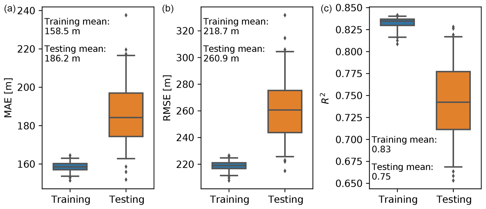
Figure 4Box and whisker plots of the metrics, including the MAE (a), RMSE (b), and R2 (c), of the eXtreme Gradient Boosting (XGB) model on the training and testing datasets. The horizontal lines show the 2.5th, 25th, 50th, 75th, and 97.5th percentiles, and the mean values are labeled in the plot.
In this study, a data-driven machine learning approach is applied to produce a spatially complete PBLH dataset. In recent years, atmospheric scientists have applied different machine learning approaches to successfully address various atmospheric problems. For example, Jiang and Zhao (2022) applied a machine learning algorithm to calculate the PBLH from GPS radio occultation data and investigated the seasonal variation in the PBLH at multiple stations. Here, we also use a machine learning approach to estimate the PBLH at the locations where no AMDAR PBLH data are available in the CONUS.
The observational dataset, consisting of the AMDAR PBLH from 13:00 to 14:00 LST from 2005 to 2019 after filtering, is shown in Fig. 2. Predictors were sampled spatially and/or temporally from ERA5 and geographical datasets. A data-driven, nonparametric model is trained to minimize the difference between model prediction and observational data, as indicated by Eq. (2):
where y is the response variable (or AMDAR PBLH here), f is an unknown function that generates response values when predictors are given, X is the predictor matrix (each column of which is a predictor), and e is the error term representing the model–observation mismatch. The learning algorithm tries to estimate the unknown function f by minimizing the sum of squares errors, eTe, plus a regularization term to reduce overfitting. Various metrics related to the model performance can be calculated using e and y, including the root-mean-square error (RMSE), the mean absolute error (MAE), and the coefficient of determination (R2). The trained model can then be used to make predictions at locations and times for which AMDAR data do not exist but predictors are available.
3.1 The eXtreme Gradient Boosting (XGB) algorithm
In this work, the XGB algorithm (Chen and Guestrin, 2016) is used to estimate the predictive function f. The XGB algorithm has been widely used in recent years to construct predictive models using complex environmental datasets (Keller et al., 2021; Masoudvaziri et al., 2021; Huang et al., 2022). We also found that XGB features better performance and faster speed than random forest, another commonly used nonparametric machine learning algorithm. The linear regression model, although the simplest and fastest, was not used because of its slightly lower performance compared with XGB (testing RMSE ∼5 % higher) and random forest (testing RMSE ∼3 % higher) as well as the fact that the computing cost of XGB is not of concern. In a regression setting of the gradient boosting framework (Friedman, 2001), the model starts with a constant value as the prediction. A shallow regression tree is then added based on the residual of the previously predicted value, and the tree’s contribution is scaled by a learning rate to reduce the variance. Following this step, new residuals are calculated, another shallow regression tree is fitted to predict these new residuals, and the contribution of this tree is scaled as done previously. This process is repeated until convergence. The XGB algorithm extends the normal gradient boosting by an optimized implementation.
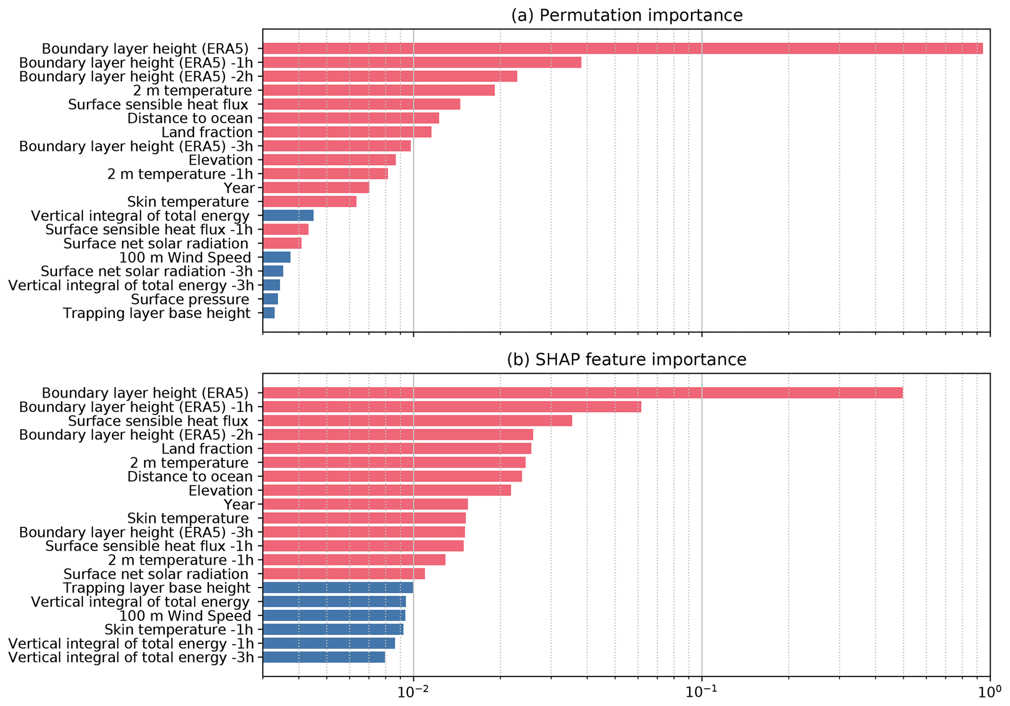
Figure 5The feature importance values calculated by permutation importance (a) and the SHapely Additive exPlanations (SHAP) approach (b). All initial predictors were included in the calculation, and only the top 20 predictors are shown. Red bars denote the predictors that are included in the final model.
3.2 Model hyperparameter tuning
The hyperparameters are external to the model and are set before the learning process begins. They are tunable and can directly affect the model performance. We found that the most sensitive hyperparameters to the XGB model were the learning rate, the number of gradient-boosted trees, and the maximum tree depth. As the model training was relatively fast, we kept the learning rate at a small value of 0.01. The number of trees and the maximum tree depth were then jointly optimized using a cross-validated grid search approach. The combinations of number of trees ranging from 200 to 1000 with a step of 100 and maximum tree depth ranging from 5 to 9 with a step of 1 were evaluated in the grid search. The cross-validation was conducted by training the XGB model using data from 46 airports randomly selected from the total 54 airports in the AMDAR data, and the remaining 8 airports for each selection were used for testing. Such a training vs. testing datasets split was repeated 100 times with the same random selector for each combination of hyperparameters. The average RMSE in the testing dataset was used as the metric. We found 800 as the number of trees and 8 as the maximum tree depth gave the best model performance. Although driven by the data, this selection yields a complicated XGB model. As the main motivation of this study is to fill the spatial gaps between AMDAR sites over the CONUS during the AMDAR period without further extrapolating in space nor time, we put more weight on the model performance than the simplicity or computational cost of the model. The MAE, RMSE, and R2 metrics using the optimized XGB hyperparameters on the training (46 airports randomly selected 100 times) and testing (the remaining 8 airports) datasets are shown in Fig. 4. The metrics on the testing datasets show higher variance, mostly because the testing datasets contain notably fewer data points than the training datasets. The overall performance of the trained model on the unseen testing datasets is only slightly lower than on the training datasets. Specifically, the R2 values indicate that, on average, the model is capable of explaining 83 % of the variation in the training datasets and 75 % of the variation in the testing datasets. We note that the interquartile ranges of the metrics' distributions on the training and testing datasets do not overlap. This indicates that a certain level of overfitting still exists and that the model may be further improved by tuning more hyperparameters (other than the number of trees and the maximum tree depth). For example, the max number of leaves is at default value, which is unlimited.
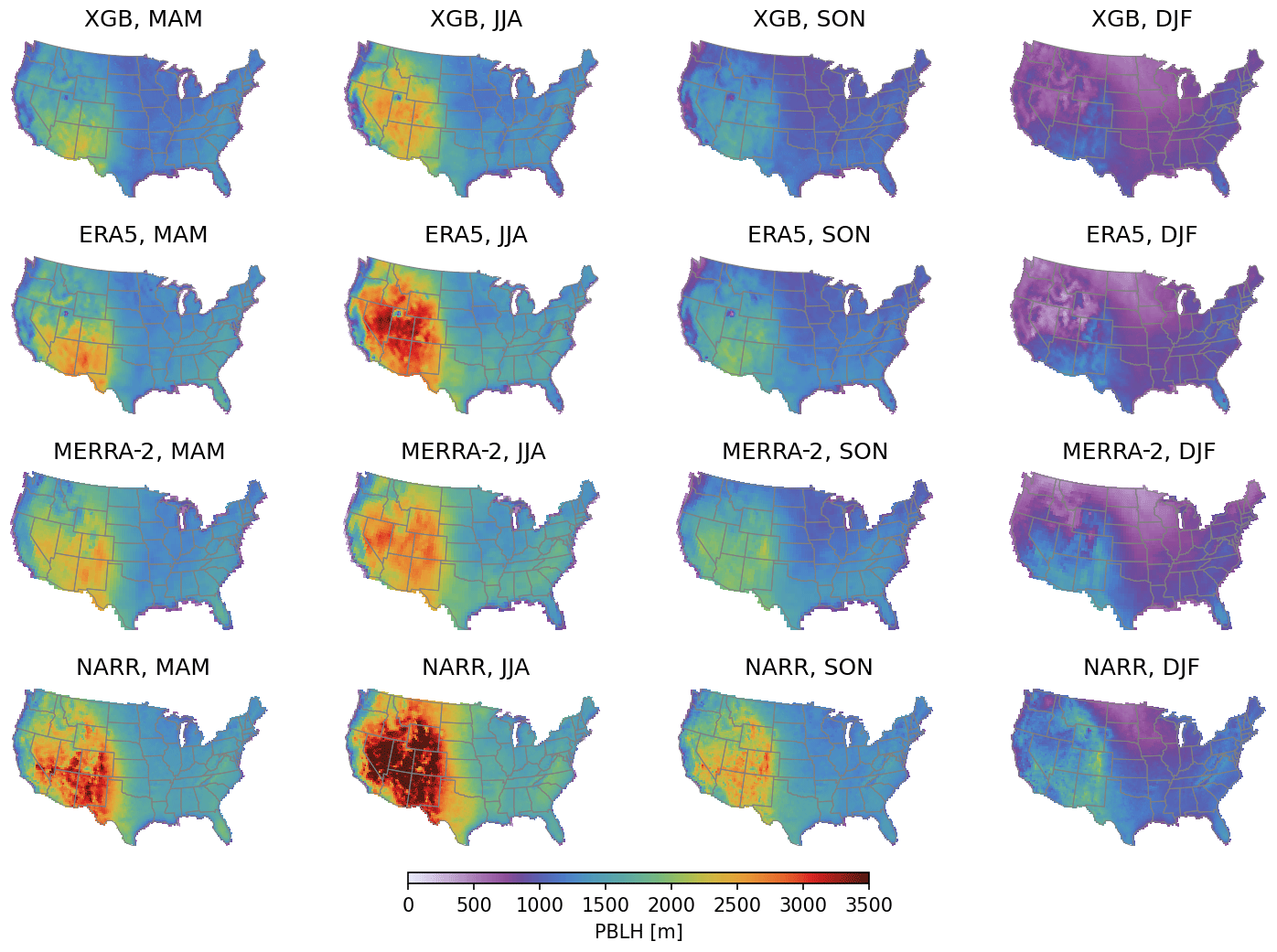
Figure 6PBLH values at 13:00–14:00 LST predicted by the XGB model and the three corresponding PBLH values from ERA5, MERRA-2, and NARR. Daily values in 2005–2019 were averaged into four seasons, as specified in the titles: March–April–May (MAM), June–July–August (JJA), September–October–November (SON), and December–January–February (DJF).
3.3 Predictor selection
A range of meteorological data fields that might contribute to predicting the AMDAR PBLH were initially selected from the ERA5 reanalysis, including its own PBLH (named boundary layer height in ERA5), surface pressure, trapping layer base height, 2 m temperature, skin temperature, cloud base height, evaporation, friction velocity, surface latent/sensible heat fluxes, surface net solar radiation, total precipitation, vertical integral of total energy, vertically integrated moisture divergence, and 100 m wind speed. Because the impacts of these environmental factors on the PBLH may not be instantaneous, these data fields were also sampled at 1, 2, and 3 h prior to the AMDAR observation time. Although the same meteorological data fields can be sampled from other model or reanalysis datasets, we found that ERA5 generally gives the best performance. Besides the meteorological factors, geographical factors were also interpolated spatially and added as predictors, including the surface elevation (Danielson and Gesch, 2011), distance to the nearest ocean coastline (NASA, 2022), and estimation of land fraction in the vicinity of the 0.25∘ × 0.3125∘ land fraction field from the GEOS-FP model (Lucchesi, 2018). In addition, we included the year and the day of year in the predictors to account for systematic observation–model mismatches with seasonal and interannual variations. In total, these add up to nearly 100 predictors. Although increasing the number of predictors will usually enhance the prediction power of the model, it is also desirable to use a parsimonious model that retains predictors that make the most physical sense. To this end, we compared the relative importance of candidate predictors by running an inclusive model with all predictors using the permutation importance and the SHapely Additive exPlanations (SHAP) approaches. The permutation feature importance is defined as the decrease in the model RMSE when the tabulated values from a single predictor are randomly shuffled (Pedregosa et al., 2011). This procedure breaks the relationship between the predictor and the response and, thus, quantifies how the model depends on the predictor. One drawback is that the permutation importance of a predictor may be underestimated if it is strongly correlated with other predictors. Correlation between predictors is significant, especially between the same meteorological data at different lag hours. As such, we also incorporated the results from the SHAP approach that computes the contribution of each feature to the prediction based on coalitional game theory while considering feature interactions (Lundberg and Lee, 2017). Figure 5 shows the relative importance of the top 20 predictors calculated using these two approaches. Although the two algorithms employ different principles, the predictors identified with leading contributions to the overall model predictive power are generally consistent. We selected 14 predictors, highlighted in red in Fig. 5, in the final model. These include the boundary layer height, 2 m temperature, sensible heat flux, skin temperature, surface net solar radiation, distance to the ocean, land fraction, elevation, and year. The significance of year as a predictor indicates interannual variations that cannot be explained by other physics-based predictors. Therefore, this model should be used during the years when AMDAR data are available. Besides the concurrent-hour boundary layer height, the boundary layer height data up to 3 h prior were included, and the 2 m temperature and surface sensible heat flux 1 h prior were also included.
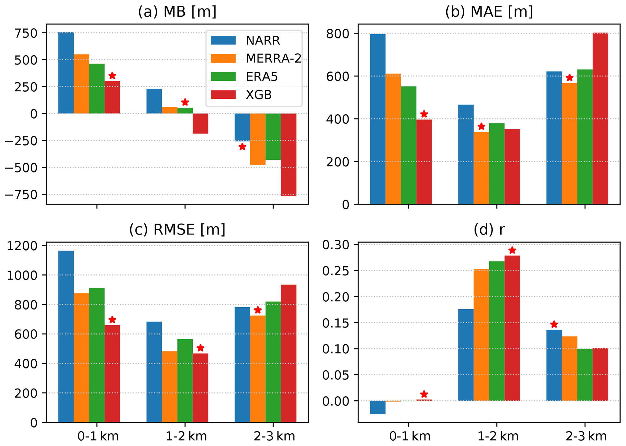
Figure 7Agreements between CALIPSO-retrieved PBLH and spatiotemporally co-located PBLH from NARR, MERRA-2, ERA5, and the XGB prediction. The CALIPSO dataset was split into ranges of 0–1, 1–2, and 2–3 km, corresponding to the three clusters of bars in each panel. The evaluation metrics include the mean bias (MB) (a), MAE (b), RMSE (c), and the Pearson correlation coefficient (d). The red star labels the dataset with the closest agreement.
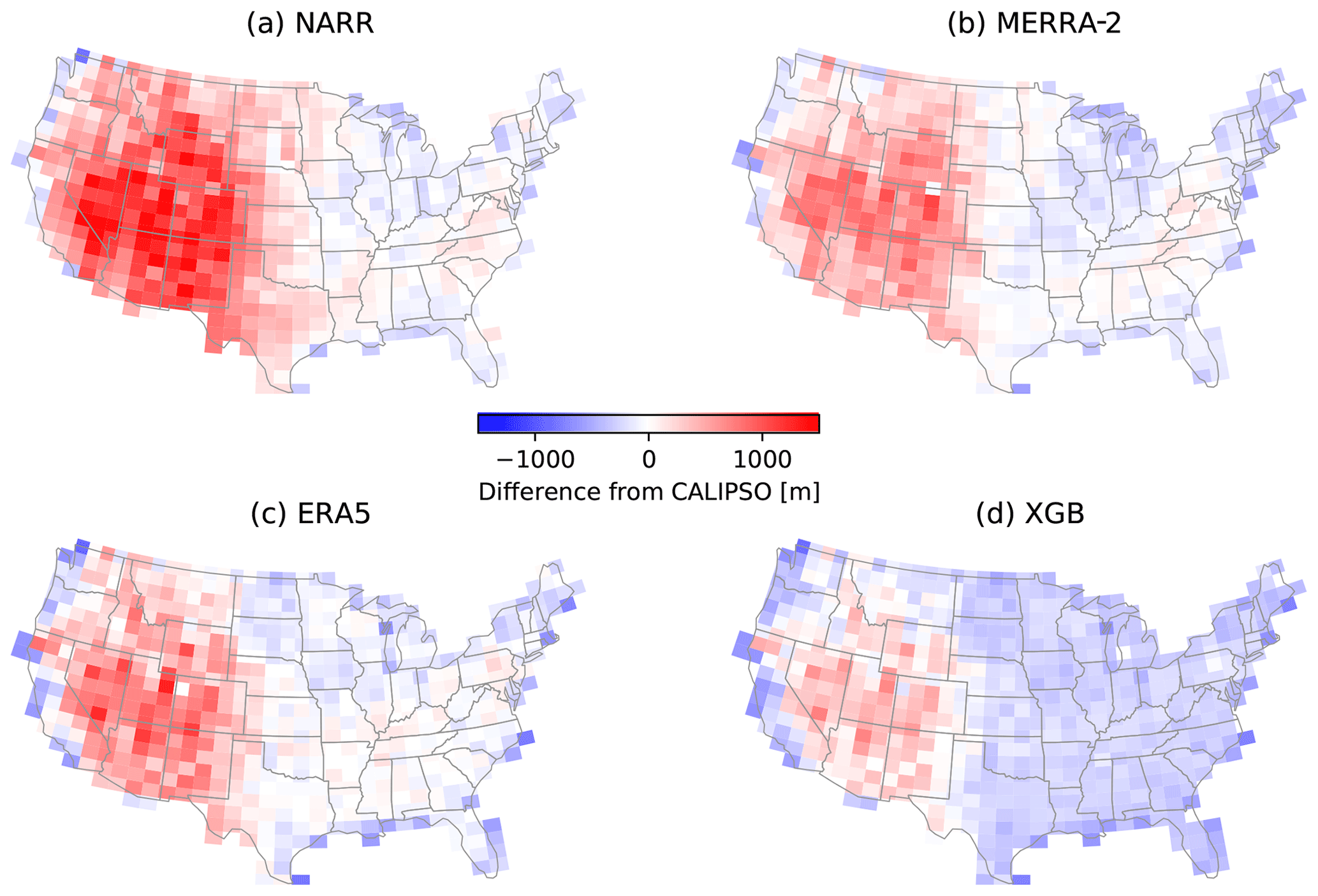
Figure 8Gridded maps of the mean biases of NARR (a), MERRA-2 (b), ERA5 (c), and XGB prediction (d) relative to CALIPSO for all available soundings of CALIPSO in 2006–2013 with a PBLH between 1 and 2 km. The spatial resolution is ∘.
3.4 Prediction of the PBLH over the CONUS
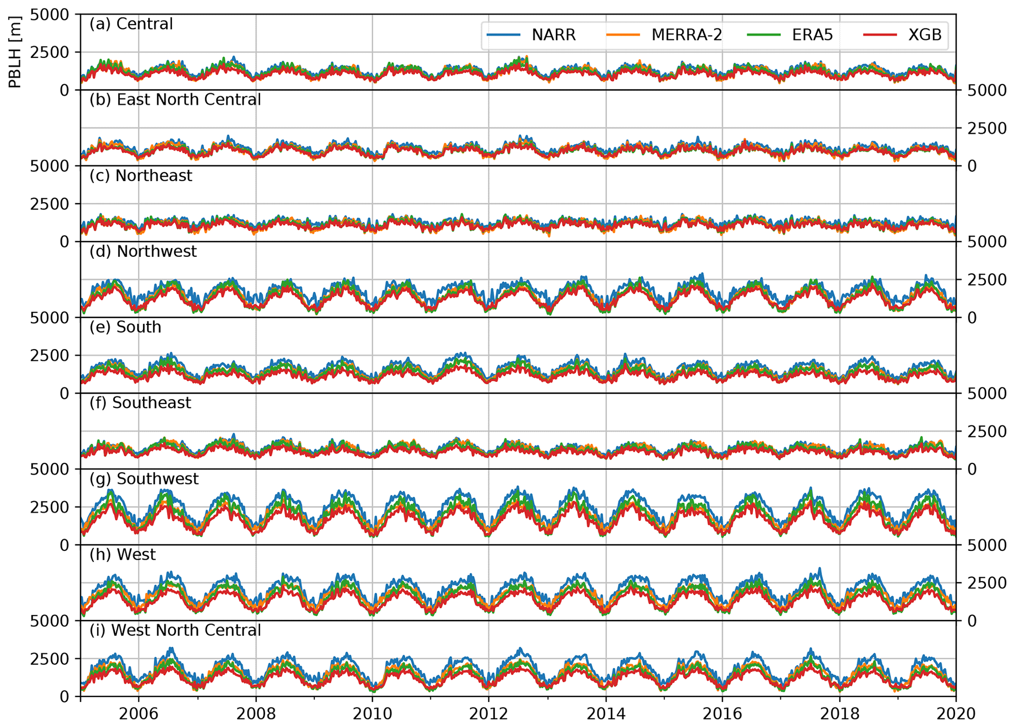
The final model with the selected hyperparameters and the predictors were trained on the entire AMDAR dataset. The trained model was then used to predict the daily PBLH at 13:00–14:00 LST throughout the 2005–2019 period. The prediction was made on the ERA5 grid points, as most predictors were already available on the same grid. Figure 6 compares the predicted daily early-afternoon PBLH in March–April–May (MAM), June–July–August (JJA), September–October–November (SON), and December–January–February (DJF) in the top row with the corresponding values from ERA5, MERRA-2, and NARR in the following rows. The predictions from the XGB model trained on the AMDAR data show very similar spatial and seasonal variation patterns to the PBLH sampled from reanalysis (ERA5, MERRA-2, and NARR). The PBLH is significantly larger in the warm season than in the cold season, and the intermountain western and southwestern areas feature a larger PBLH than other regions. The XGB-model-predicted PBLH is lower than the PBLH from the three reanalysis products in all four seasons. This result is consistent with the direct comparison between the AMDAR PBLH and the co-located ERA5 PBLH made by Zhang et al. (2020). We also look into finer-grained intercomparisons by averaging over nine different climate regions in the CONUS (Karl and Koss, 1984) at a weekly resolution (i.e., weekly averages of the PBLH at 13:00–14:00 LST). The results are shown in Fig. A1 and are consistent with the seasonal maps shown in Fig. 6.
Because the locations of AMDAR airports are sparse over the CONUS (Fig. 1a), it is important to evaluate the performance of the XGB model trained by AMDAR data. In addition to the XGB-predicted PBLH, we also used spatiotemporally interpolated PBLH fields from NARR, MERRA-2, and ERA5 and included them in the evaluations against independent observational datasets.
4.1 The predicted PBLH vs. CALIPSO
The agreement between the CALIPSO PBLH and the four datasets to be evaluated (the NARR, MERRA-2, and ERA5 reanalyses as well as the XGB prediction) is strongly dependent on the ranges of the PBLH. Figure 7 compares the mean bias (MB), MAE, RMSE, and the Pearson correlation coefficient (r) between CALIPSO and these datasets with the comparisons split for the CALIPSO PBLH at 0–1, 1–2, and 2–3 km. The dataset with the best performance (MB closest to 0, lowest MAE and RMSE, and highest r) is marked with a red star. When the CALIPSO PBLH is below 1 km, there is little correlation between CALIPSO and any other datasets (Fig. 7d), indicating that the CALIPSO retrieval might be unreliable at a low PBLH. Furthermore, the overall agreement for the 2–3 km range is lower than its counterpart for the 1–2 km range. The distribution of the CALIPSO PBLH, as shown in Fig. 3a, is quite different from that of the AMDAR PBLH, with a larger contribution in the 2–3 km range. This may mean that the worst performance by the XGB prediction when the CALIPSO PBLH is at 2–3 km can be explained by the lack of training AMDAR data in this range. However, the performance of the three reanalysis datasets is also counterintuitive, as the NARR PBLH is one of the top performers here but is the least accurate in the following comparisons with airborne data (see below). This lack of coherence among datasets for PBLHs above 2 km suggests that CALIPSO retrieval might also be subject to systematic errors at these high values. As such, we focus on the CALIPSO PBLH in the range of 1–2 km. In this range, the XGB prediction shows the best RMSE and correlation, a competitive MAE, and a negative bias relative to CALIPSO. Moreover, the XGB prediction outperforms ERA5 in terms of MAE, RMSE, and correlation coefficient, demonstrating the effectiveness of model training using AMDAR data.
A key strength of the CALIPSO dataset is its relatively uniform spatial distribution (Fig. 1b), which may help identify spatial patterns in the model prediction bias, especially in regions where AMDAR coverage is low. Figure 8 maps the bias between the four evaluated datasets and CALIPSO, binned in ∘ grid boxes over the CONUS. The comparisons were limited to cases with a CALIPSO PBLH of 1–2 km, corresponding to the middle cluster of bars in Fig. 7. All four evaluated datasets show a high bias relative to CALIPSO in the western CONUS, except near the coastline. This high bias is the largest in NARR, whereas it is minimal in the XGB prediction. These high biases in the reanalysis PBLHs have also been noted by previous comparison studies (McGrath-Spangler and Denning, 2012; Zhang et al., 2020). The reanalysis datasets are in general agreement with CALIPSO in low-elevation regions in the east, whereas the XGB predictions show a near-uniform low bias of 100–200 m. This contributes to an overall low bias of XGB prediction relative to CALIPSO (Fig. 7a, middle cluster). As shown in the following comparisons with airborne data, the MB values of the XGB prediction relative to the reference datasets are generally lower than the reanalysis datasets and are closer to zero. Hence, a possible explanation is that CALIPSO is slightly biased high due to aerosol distributions above the PBL top. The spatial distribution of the XGB prediction bias relative to CALIPSO does not show more significant systematic features than the biases of the three reanalysis datasets, indicating that the spatial extrapolation of the AMDAR PBLH through the meteorological and geographical features does not introduce excessive errors.
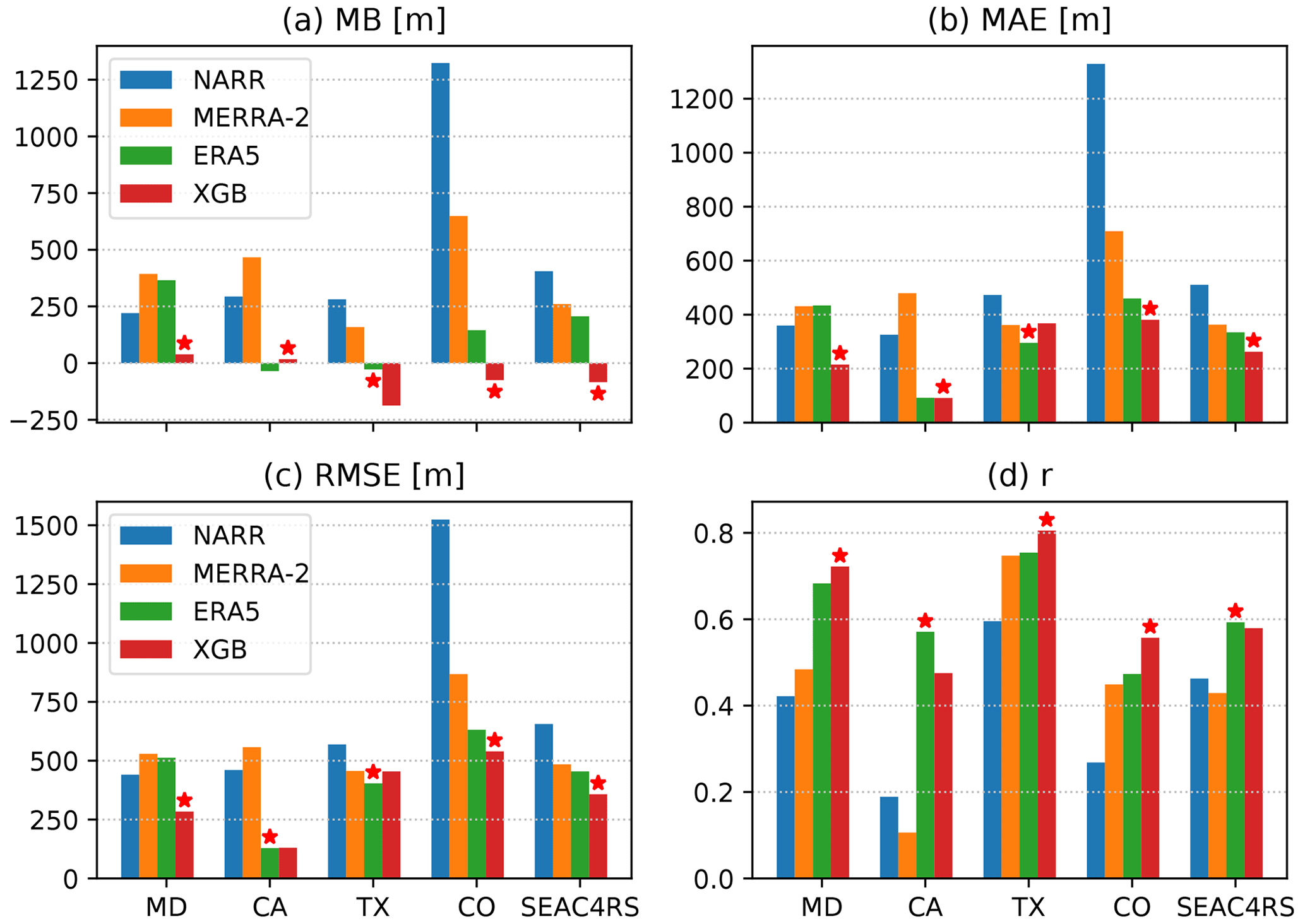
Figure 9Similar to Fig. 7 but using the HSRL PBLH measurements during five airborne campaigns as the reference dataset. Each campaign corresponds to a cluster of bars in each panel.
4.2 The predicted PBLH vs. HSRL
The same metrics were used for an evaluation against the HSRL measurements during the DISCOVER-AQ and SEAC4RS campaigns, as shown in Fig. 9. The XGB prediction shows a lower MB than all of the reanalysis datasets in four out of five campaigns, with DISCOVER-AQ TX being the only exception. The reanalysis datasets show large positive biases relative to HSRL in DISCOVER-AQ CO and SEAC4CRS, likely due to the large-scale positive biases in the western CONUS seen in Fig. 8a–c. The XGB prediction gives the best performance in four out of five campaigns (MD, CA, CO, and SEAC4CRS) in terms of MAE, three out of five campaigns (MD, CO, and SEAC4CRS) in terms of RMSE, and three out of five campaigns (MD, TX, and CO) in terms of correlation coefficient. The ERA5 is the top performer for all cases where the XGB prediction is not at the top. Overall, the ERA5 PBLH demonstrates remarkably better agreement with observations than NARR and MERRA-2. The performance of XGB prediction is robustly improved over ERA5 during DISCOVER-AQ MD, which is attributed to the high airport density in the northeast (Fig. 1a). The XGB prediction, however, does not significantly improve over ERA5 during DISCOVER-AQ CA. A likely reason for this is that the airborne sampling was limited to the San Joaquin Valley where no AMDAR data were available from Zhang et al. (2019).
Compared with the evaluation using the CALIPSO PBLH in the previous section, the correlations between the evaluated datasets and the airborne HSRL-retrieved PBLH are substantially better. The correlation coefficient between XGB prediction and HSRL during DISCOVER-AQ TX is 0.8, while the HSRL PBLH spans a broad range from below 1 to 3 km (Fig. 3i). The correlation coefficients using CALIPSO are below 0.3 for all cases (Fig. 7d). Therefore, although both the HSRL and CALIPSO PBLH are retrieved from aerosol backscatter gradients, the HSRL dataset is likely to have significantly better quality.
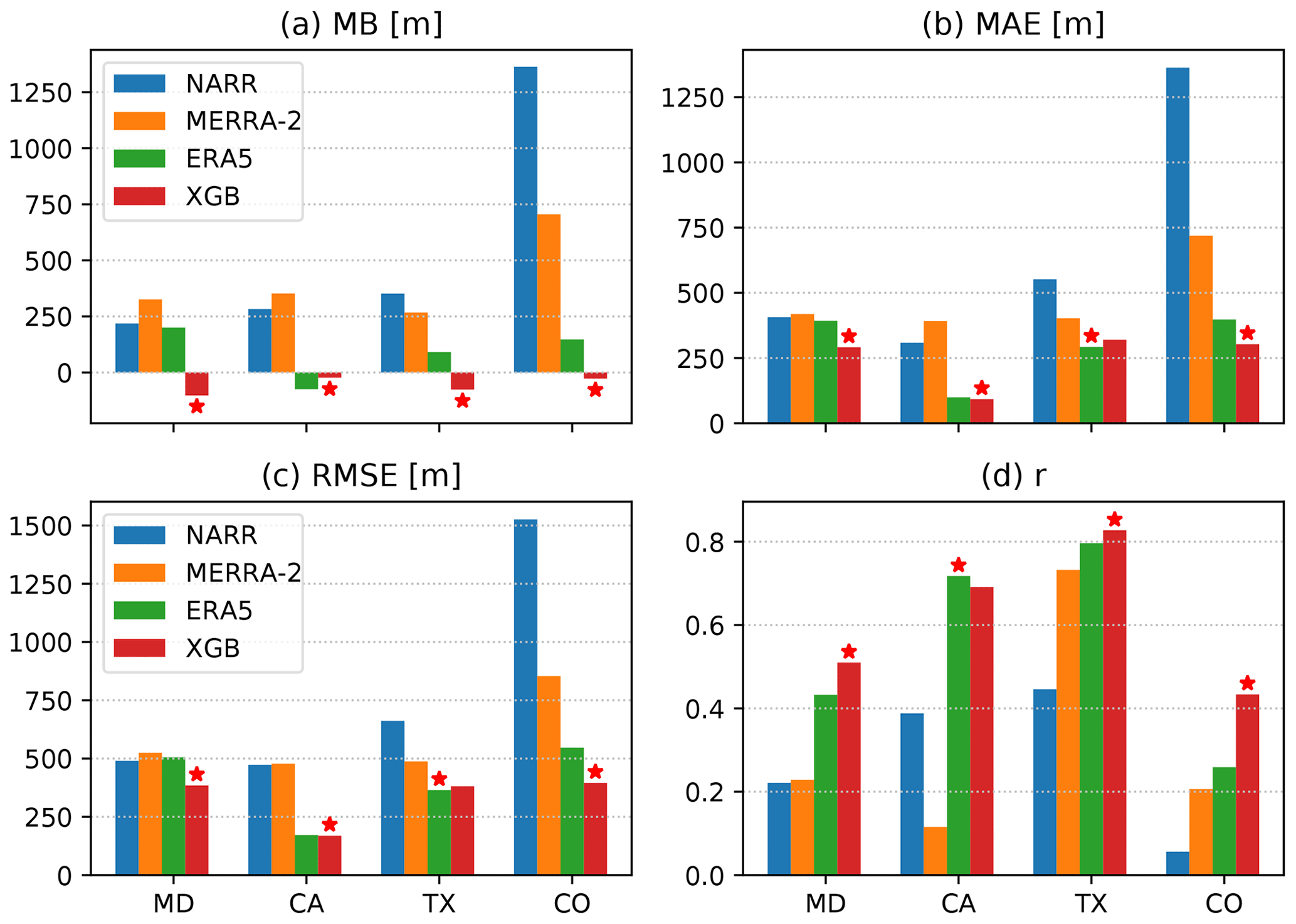
4.3 The predicted PBLH vs. spiral profiles
During the four DISCOVER-AQ campaigns, the PBLH was manually labeled from spiral profiles measured in situ by aircraft. The comparisons between this PBLH observation dataset and the four evaluated datasets (NARR, MERRA-2, ERA5, and XGB prediction) are very similar to the comparisons using the HSRL dataset and are shown in Fig. 10. This similarity is consistent with the resemblance of the distributions of the spiral-profile- and HSRL-based PBLH (comparing Fig. 3b–e with Fig. 3g–j). The XGB prediction gives the best MB in all campaigns, the lowest MAE and RMSE in all campaigns except DISCOVER-AQ TX, and the highest correlation coefficient in all campaigns except DISCOVER-AQ CA.
Overall, the XGB prediction shows significantly better agreement with the three independent observational datasets than the reanalysis datasets, for which the ERA5 performs better than MERRA-2 and NARR. The XGB prediction outperforms ERA5 in most cases, mostly notably in DISCOVER-AQ MD where AMDAR airports are relatively dense.
We developed a data-driven machine learning model to predict the spatially complete PBLH over the CONUS daily at 13:00–14:00 LST using AMDAR data at 54 airport locations from 2005 to 2019 (Zhang et al., 2019). The XGB algorithm was used to train the regression model with predictors mostly selected from the ERA5 reanalysis. The model hyperparameters were optimized using cross-validated grid search by randomly splitting the airports into training and testing datasets. The predicted PBLH was evaluated using independent PBLH observations from CALIPSO, HSRL, and spiral profiles during the DISCOVER-AQ campaigns, with the caveat that different PBLH products and estimates have different ways of computing the PBLH and that PBLH observations used in these evaluation are sparse and subject to various uncertainties and inconsistency in retrieval methodology. The predicted PBLH is generally in better agreement with the evaluation datasets than the PBLH sampled from reanalysis (NARR, MERRA-2, and ERA5). The reanalysis datasets give a higher PBLH in the western CONUS relative to the evaluation datasets.
While this work demonstrates the potential use of data-driven approaches in deriving the spatially complete PBLH, significant challenges still exist due to the uncertainty in existing datasets. We observe clusters of AMDAR observations that are uncorrelated with the co-located ERA5 PBLH, mostly under stable conditions, and we find that no meteorological or geographical factors could explain this discrepancy. A preprocessing step that filters out these data clusters had to be implemented to mitigate their impacts on model training. Consequently, the model is trained and tested on a subset of AMDAR data and does not fully represent the entire AMDAR dataset. Moreover, the model configurations have been specifically optimized and evaluated to generate the spatially complete PBLH dataset over the CONUS during the period when AMDAR PBLH data are available (2005–2019). Further generalization of the work will require additional tuning and model evaluation. Also note that the modeling in this work focused on the entire CONUS. Further improvements in model performance may be achieved by focusing on smaller geographic regions and fine-tuning region-specific predictors.
The satellite-based CALIPSO dataset is the most spatiotemporally complete for model evaluation, but it is subject to large uncertainties, providing essentially no correlations with reanalysis datasets and the prediction from this work when the PBLH is lower than 1 km. Future spaceborne PBLH observations with higher fidelity and more routine suborbital measurements, especially under stable conditions, will be beneficial.
This work extends the AMDAR-based PBLH data from Zhang et al. (2020), which are only available at point locations, to the entire CONUS, enabling sampling of the PBLH at the sounding locations and times of low-Earth orbit spaceborne sensors with an overpass time in the early afternoon. As the AMDAR PBLH data are available hourly, it is possible to extend this work to other daytime hours and even nighttime hours with the caution that it will be more challenging due to the increase in stable conditions and the fewer observational datasets available for evaluation. The HSRL and spiral-profile PBLH observations will also be available for other daytime hours but CALIPSO observations will not. This extension will synergize with satellite atmospheric composition observations in the morning orbits and the TEMPO mission that covers North America at an hourly resolution (Zoogman et al., 2017).
The AMDAR data are available through the Meteorological Assimilation Data Ingest System web service portal at https://madis-data.cprk.ncep.noaa.gov/madisPublic1/data/archive/ (last access: 15 July 2022; NOAA, 2023). The hourly boundary layer profiles and PBLH based on AMDAR data can be found at https://doi.org/10.5281/zenodo.3934378 (Li, 2020). The ERA5 data are available from the Copernicus Climate Data Store at https://cds.climate.copernicus.eu/cdsapp#!/dataset/reanalysis-era5-single-levels?tab=form (last access: 15 July 2022; ECMWF Support Portal, 2018). The MERRA-2 data are available through the NASA GES DISC at https://disc.gsfc.nasa.gov/datasets/M2T1NXSLV_5.12.4/summary (last access: 15 July 2022; Global Modeling and Assimilation Office, 2015). The NARR data are available from the NCAR Research Data Archive at https://rda.ucar.edu/datasets/ds608.0/ (last access: 15 July 2022; National Centers for Environmental Prediction/National Weather Service/NOAA/U.S. Department of Commerce, 2005). The CALIPSO data are available through the University of Wisconsin–Madison Space Science and Engineering Center website (https://download.ssec.wisc.edu/files/calipso/, last access: 15 July 2022; SSEC, 2023). The DISCOVER-AQ data are available at https://doi.org/10.5067/Aircraft/DISCOVER-AQ/Aerosol-TraceGas (NASA Langley Research Center's (LaRC) ASDC DAAC, 2023), and the SEAC4RS data are available at https://doi.org/10.5067/Aircraft/SEAC4RS/Aerosol-TraceGas-Cloud (NASA, 2023).
ST, DL, and KS developed the methodology. ZA, ST, and KS performed the analysis and wrote the paper. ZA and KS managed the datasets. AJS provided expertise on airborne lidar measurements. RK provided expertise on spaceborne lidar measurements. All co-authors contributed to editing the paper.
The authors declare that they have no conflict of interest.
Publisher’s note: Copernicus Publications remains neutral with regard to jurisdictional claims in published maps and institutional affiliations.
This research has been supported by the NASA Atmospheric Composition Modeling and Analysis Program (ACMAP). We thank Mingchen Gao at the University at Buffalo for helpful discussions.
This research has been supported by the NASA Earth Sciences Division (grant no. 80NSSC19K0988).
This paper was edited by Laura Bianco and reviewed by Joseph Santanello and one anonymous referee.
Angevine, W. M., Eddington, L., Durkee, K., Fairall, C., Bianco, L., and Brioude, J.: Meteorological model evaluation for CalNex 2010, Mon. Weather Rev., 140, 3885–3906, 2012. a
Boersma, K. F., Jacob, D. J., Trainic, M., Rudich, Y., DeSmedt, I., Dirksen, R., and Eskes, H. J.: Validation of urban NO2 concentrations and their diurnal and seasonal variations observed from the SCIAMACHY and OMI sensors using in situ surface measurements in Israeli cities, Atmos. Chem. Phys., 9, 3867–3879, https://doi.org/10.5194/acp-9-3867-2009, 2009. a
Chen, T. and Guestrin, C.: Xgboost: A scalable tree boosting system, in: Proceedings of the 22nd acm sigkdd international conference on knowledge discovery and data mining, 13–17 August 2016, San Francisco, CA, https://doi.org/10.1145/2939672, 785–794, 2016. a
Danielson, J. J. and Gesch, D. B.: Global multi-resolution terrain elevation data 2010 (GMTED2010), Tech. rep., USGS, https://doi.org/10.3133/ofr20111073, 2011. a
Davis, K. J., Gamage, N., Hagelberg, C. R., Kiemle, C., Lenschow, D. H., and Sullivan, P. P.: An Objective Method for Deriving Atmospheric Structure from Airborne Lidar Observations, J. Atmos. Ocean. Technol., 17, 1455–1468, https://doi.org/10.1175/1520-0426(2000)017<1455:AOMFDA>2.0.CO;2, 2000. a
ECMWF: Part IV: Physical processes, in: IFS Documentation CY43R3, IFS Documentation, ECMWF, https://www.ecmwf.int/node/17736 (last access: 15 July 2022), 2017. a
ECMWF Support Portal: ERA5 hourly data on single levels from 1959 to present, ECMWF [data set], https://cds.climate.copernicus.eu/cdsapp#!/dataset/reanalysis-era5-single-levels?tab=form (last access: 15 July 2022), 2018. a
ECMWF: ERA5 hourly data on single levels from 1979 to present, https://doi.org/10.24381/cds.adbb2d47, 2020. a
Friedman, J. H.: Greedy function approximation: a gradient boosting machine, Annals of statistics, ISSN 00905364, 1189–1232, 2001. a
Garratt, J. R.: The atmospheric boundary layer, Earth-Sci. Rev., 37, 89–134, 1994. a
Gelaro, R., McCarty, W., Suárez, M. J., Todling, R., Molod, A., Takacs, L., Randles, C. A., Darmenov, A., Bosilovich, M. G., and Reichle, R.: The modern-era retrospective analysis for research and applications, version 2 (MERRA-2), J. Climate, 30, 5419–5454, 2017. a
Gerbig, C., Körner, S., and Lin, J. C.: Vertical mixing in atmospheric tracer transport models: error characterization and propagation, Atmos. Chem. Phys., 8, 591–602, https://doi.org/10.5194/acp-8-591-2008, 2008. a
Global Modeling and Assimilation Office (GMAO): MERRA-2 tavg1_2d_slv_Nx: 2d,1-Hourly,Time-Averaged,Single-Level,Assimilation,Single-Level Diagnostics V5.12.4, Greenbelt, MD, USA, Goddard Earth Sciences Data and Information Services Center (GES DISC), https://doi.org/10.5067/VJAFPLI1CSIV, 2015. a
GMAO: MERRA-2 tavg1_2d_slv_Nx: 2d,1-Hourly,Time-Averaged,Single-Level,Assimilation,Single-Level Diagnostics V5.12.4, Greenbelt, MD, USA, Goddard Earth Sciences Data and Information Services Center (GES DISC), https://doi.org/10.5067/VJAFPLI1CSIV, 2015. a
Guo, J., Miao, Y., Zhang, Y., Liu, H., Li, Z., Zhang, W., He, J., Lou, M., Yan, Y., Bian, L., and Zhai, P.: The climatology of planetary boundary layer height in China derived from radiosonde and reanalysis data, Atmos. Chem. Phys., 16, 13309–13319, https://doi.org/10.5194/acp-16-13309-2016, 2016. a
Hair, J. W., Hostetler, C. A., Cook, A. L., Harper, D. B., Ferrare, R. A., Mack, T. L., Welch, W., Izquierdo, L. R., and Hovis, F. E.: Airborne high spectral resolution lidar for profiling aerosol optical properties, Appl. Opt., 47, 6734–6752, 2008. a
Hegarty, J. D., Lewis, J., McGrath-Spangler, E. L., Henderson, J., Scarino, A. J., DeCola, P., Ferrare, R., Hicks, M., Adams-Selin, R. D., and Welton, E. J.: Analysis of the Planetary Boundary Layer Height during DISCOVER-AQ Baltimore–Washington, D.C., with Lidar and High-Resolution WRF Modeling, J. Appl. Meteorol. Climatol., 57, 2679–2696, https://doi.org/10.1175/JAMC-D-18-0014.1, 2018. a, b, c, d
Hersbach, H., Bell, B., Berrisford, P., Hirahara, S., Horányi, A., Muñoz-Sabater, J., Nicolas, J., Peubey, C., Radu, R., Schepers, D., Simmons, A., Soci, C., Abdalla, S., Abellan, X., Balsamo, G., Bechtold, P., Biavati, G., Bidlot, J., Bonavita, M., De Chiara, G., Dahlgren, P., Dee, D., Diamantakis, M., Dragani, R., Flemming, J., Forbes, R., Fuentes, M., Geer, A., Haimberger, L., Healy, S., Hogan, R. J., Hólm, E., Janisková, M., Keeley, S., Laloyaux, P., Lopez, P., Lupu, C., Radnoti, G., de Rosnay, P., Rozum, I., Vamborg, F., Villaume, S., and Thépaut, J.-N.: The ERA5 global reanalysis, Q. J. Roy. Meteorol. Soc., 146, 730, https://doi.org/10.1002/qj.3803, 2020. a
Hirschi, M., Seneviratne, S. I., Alexandrov, V., Boberg, F., Boroneant, C., Christensen, O. B., Formayer, H., Orlowsky, B., and Stepanek, P.: Observational evidence for soil-moisture impact on hot extremes in southeastern Europe, Nat. Geosci., 4, 17–21, 2011. a
Hu, L., Jacob, D. J., Liu, X., Zhang, Y., Zhang, L., Kim, P. S., Sulprizio, M. P., and Yantosca, R. M.: Global budget of tropospheric ozone: Evaluating recent model advances with satellite (OMI), aircraft (IAGOS), and ozonesonde observations, Atmos. Environ., 167, 323–334, 2017. a
Huang, C., Sun, K., Hu, J., Xue, T., Xu, H., and Wang, M.: Estimating 2013–2019 NO2 exposure with high spatiotemporal resolution in China using an ensemble model, Environ. Pollut., 292, 118285, https://doi.org/10.1016/j.envpol.2021.118285, 2022. a
Jiang, R. and Zhao, K.: Using machine learning method on calculation of boundary layer height, Neural Comput. Appl., 34, 2597–2609, 2022. a
Jordan, N. S., Hoff, R. M., and Bacmeister, J. T.: Validation of Goddard Earth Observing System-version 5 MERRA planetary boundary layer heights using CALIPSO, J. Geophys. Res.-Atmos., 115, D24, https://doi.org/10.1029/2009JD013777, 2010. a
Karl, T. and Koss, W. J.: Regional and national monthly, seasonal, and annual temperature weighted by area, 1895–1983, https://repository.library.noaa.gov/view/noaa/10238 (last access: 15 July 2022), 1984. a
Keller, C. A., Evans, M. J., Knowland, K. E., Hasenkopf, C. A., Modekurty, S., Lucchesi, R. A., Oda, T., Franca, B. B., Mandarino, F. C., Díaz Suárez, M. V., Ryan, R. G., Fakes, L. H., and Pawson, S.: Global impact of COVID-19 restrictions on the surface concentrations of nitrogen dioxide and ozone, Atmos. Chem. Phys., 21, 3555–3592, https://doi.org/10.5194/acp-21-3555-2021, 2021. a
Laughner, J. L., Zhu, Q., and Cohen, R. C.: Evaluation of version 3.0B of the BEHR OMI NO2 product, Atmos. Meas. Tech., 12, 129–146, https://doi.org/10.5194/amt-12-129-2019, 2019. a, b
Lee, T. R. and De Wekker, S. F. J.: Estimating Daytime Planetary Boundary Layer Heights over a Valley from Rawinsonde Observations at a Nearby Airport: An Application to the Page Valley in Virginia, United States, J. Appl. Meteorol. Climatol., 55, 791–809, https://doi.org/10.1175/JAMC-D-15-0300.1, 2016. a
Li, D.: AMDAR_BL_PBLH_DATASET (v1.0), Zenodo [data set], https://doi.org/10.5281/zenodo.3934378, 2020. a
Lu, X., Jacob, D. J., Zhang, Y., Maasakkers, J. D., Sulprizio, M. P., Shen, L., Qu, Z., Scarpelli, T. R., Nesser, H., Yantosca, R. M., Sheng, J., Andrews, A., Parker, R. J., Boesch, H., Bloom, A. A., and Ma, S.: Global methane budget and trend, 2010–2017: complementarity of inverse analyses using in situ (GLOBALVIEWplus CH4 ObsPack) and satellite (GOSAT) observations, Atmos. Chem. Phys., 21, 4637–4657, https://doi.org/10.5194/acp-21-4637-2021, 2021. a, b
Lucchesi, R.: File Specification for GEOS-5 FP (Forward Processing), https://gmao.gsfc.nasa.gov/GMAO_products/documents/GEOS_5_FP_File_Specification_ON4v1_2.pdf (last access: 15 July 2022), 2018. a
Lundberg, S. M. and Lee, S.-I.: A unified approach to interpreting model predictions, Advances in neural information processing systems, 30, https://proceedings.neurips.cc/paper/2017/file/8a20a8621978632d76c43dfd28b67767-Paper.pdf (last access: 15 July 2022), 2017. a
Masoudvaziri, N., Ganguly, P., Mukherjee, S., and Sun, K.: Impact of geophysical and anthropogenic factors on wildfire size: a spatiotemporal data-driven risk assessment approach using statistical learning, Stoch. Environ. Res. Risk Assess., 36, 1103–1129, https://doi.org/10.1007/s00477-021-02087-w, 2021. a
McGrath-Spangler, E. L. and Denning, A. S.: Estimates of North American summertime planetary boundary layer depths derived from space-borne lidar, J. Geophys. Res.-Atmos., 117, D15, https://doi.org/10.1029/2012JD017615, 2012. a, b, c
McGrath-Spangler, E. L. and Denning, A. S.: Global seasonal variations of midday planetary boundary layer depth from CALIPSO space-borne LIDAR, J. Geophys. Res.-Atmos., 118, 1226–1233, https://doi.org/10.1002/jgrd.50198, 2013. a
McGrath-Spangler, E. L. and Molod, A.: Comparison of GEOS-5 AGCM planetary boundary layer depths computed with various definitions, Atmos. Chem. Phys., 14, 6717–6727, https://doi.org/10.5194/acp-14-6717-2014, 2014. a
McKain, K., Wofsy, S. C., Nehrkorn, T., Eluszkiewicz, J., Ehleringer, J. R., and Stephens, B. B.: Assessment of ground-based atmospheric observations for verification of greenhouse gas emissions from an urban region., P. Natl. Acad. Sci. USA, 109, 8423–8428, https://doi.org/10.1073/pnas.1116645109, 2012. a
Mesinger, F., DiMego, G., Kalnay, E., Mitchell, K., Shafran, P. C., Ebisuzaki, W., Jović, D., Woollen, J., Rogers, E., and Berbery, E. H.: North American regional reanalysis, B. Am. Meteorol. Soc., 87, 343–360, 2006. a
Millet, D. B., Baasandorj, M., Farmer, D. K., Thornton, J. A., Baumann, K., Brophy, P., Chaliyakunnel, S., de Gouw, J. A., Graus, M., Hu, L., Koss, A., Lee, B. H., Lopez-Hilfiker, F. D., Neuman, J. A., Paulot, F., Peischl, J., Pollack, I. B., Ryerson, T. B., Warneke, C., Williams, B. J., and Xu, J.: A large and ubiquitous source of atmospheric formic acid, Atmos. Chem. Phys., 15, 6283–6304, https://doi.org/10.5194/acp-15-6283-2015, 2015. a
Moninger, W. R., Mamrosh, R. D., and Pauley, P. M.: Automated meteorological reports from commercial aircraft, B. Am. Meteorol. Soc., 84, 203–216, 2003. a
Murray, L. T., Leibensperger, E. M., Orbe, C., Mickley, L. J., and Sulprizio, M.: GCAP 2.0: a global 3-D chemical-transport model framework for past, present, and future climate scenarios, Geosci. Model Dev., 14, 5789–5823, https://doi.org/10.5194/gmd-14-5789-2021, 2021. a, b
NASA: Distance to the Nearest Coast, NASA, https://oceancolor.gsfc.nasa.gov/docs/distfromcoast/ (last access: 15 July 2022), 2022. a
NASA: SEAC4RS – Studies of Emissions and Atmospheric Composition, Clouds and Climate Coupling by Regional Surveys, NASA [data set], https://doi.org/10.5067/Aircraft/SEAC4RS/Aerosol-TraceGas-Cloud, 2023. a
NASA Langley Research Center's (LaRC) ASDC DAAC: Deriving Information on Surface Conditions from Column and Vertically Resolved Observations Relevant to Air Quality, NASA [data set], https://doi.org/10.5067/Aircraft/DISCOVER-AQ/Aerosol-TraceGas, 2023. a
National Centers for Environmental Prediction/National Weather Service/NOAA/U.S. Department of Commerce: updated monthly, NCEP North American Regional Reanalysis (NARR), Research Data Archive at the National Center for Atmospheric Research, Computational and Information Systems Laboratory, NOAA [data set], https://rda.ucar.edu/datasets/ds608.0/ (last access: 15 July 2022), 2005. a
NCEP: NCEP North American Regional Reanalysis (NARR), NCEP, https://rda.ucar.edu/datasets/ds608.0/ (last access: 15 July 2022), 2005. a
NOAA: Index of /madisPublic1/data/archive, NOAA [data set], https://madis-data.cprk.ncep.noaa.gov/madisPublic1/data/archive/ (last access: 15 July 2022), 2023. a
Pedregosa, F., Varoquaux, G., Gramfort, A., Michel, V., Thirion, B., Grisel, O., Blondel, M., Prettenhofer, P., Weiss, R., Dubourg, V., Vanderplas, J., Passos, A., Cournapeau, D., Brucher, M., Perrot, M., and Duchesnay, E.: Scikit-learn: Machine Learning in Python, J. Mach. Learn. Res., 12, 2825–2830, 2011. a
Santanello, J. A., Peters-Lidard, C. D., Kennedy, A., and Kumar, S. V.: Diagnosing the nature of land–atmosphere coupling: A case study of dry/wet extremes in the US southern Great Plains, Jo. Hydrometeorol., 14, 3–24, 2013. a
Santanello, J. A., Roundy, J., and Dirmeyer, P. A.: Quantifying the land–atmosphere coupling behavior in modern reanalysis products over the US Southern Great Plains, J. Climate, 28, 5813–5829, 2015. a
Santanello, J. A., Dirmeyer, P. A., Ferguson, C. R., Findell, K. L., Tawfik, A. B., Berg, A., Ek, M., Gentine, P., Guillod, B. P., Van Heerwaarden, C., Roundy J., and Wulfmeyer V.: Land–atmosphere interactions: The LoCo perspective, B. Am. Meteorol. Soc., 99, 1253–1272, 2018. a
Scarino, A. J., Obland, M. D., Fast, J. D., Burton, S. P., Ferrare, R. A., Hostetler, C. A., Berg, L. K., Lefer, B., Haman, C., Hair, J. W., Rogers, R. R., Butler, C., Cook, A. L., and Harper, D. B.: Comparison of mixed layer heights from airborne high spectral resolution lidar, ground-based measurements, and the WRF-Chem model during CalNex and CARES, Atmos. Chem. Phys., 14, 5547–5560, https://doi.org/10.5194/acp-14-5547-2014, 2014. a
Seidel, D. J., Zhang, Y., Beljaars, A., Golaz, J.-C., Jacobson, A. R., and Medeiros, B.: Climatology of the planetary boundary layer over the continental United States and Europe, J. Geophys. Res.-Atmos., 117, D17, https://doi.org/10.1029/2012JD018143, 2012. a, b
SSEC: CALIPSO, SSEC [data set], https://download.ssec.wisc.edu/files/calipso/, last access: 15 July 2022, 2023. a
Stensrud, D. J.: Parameterization schemes: keys to understanding numerical weather prediction models, Cambridge University Press, 449 pp., https://doi.org/10.1017/CBO9780511812590, 2009. a
Stull, R. B.: An introduction to boundary layer meteorology, Kluwer Academic, 666 pp., https://doi.org/10.1007/978-94-009-3027-8, 1988. a
Su, T., Li, Z., and Kahn, R.: Relationships between the planetary boundary layer height and surface pollutants derived from lidar observations over China: regional pattern and influencing factors, Atmos. Chem. Phys., 18, 15921–15935, https://doi.org/10.5194/acp-18-15921-2018, 2018. a, b
Sun, K., Cady-Pereira, K., Miller, D. J., Tao, L., Zondlo, M., Nowak, J., Neuman, J. A., Mikoviny, T., Muller, M., Wisthaler, A., Scarino, A. J., and Hostetler, C.: Validation of TES ammonia observations at the single pixel scale in the San Joaquin Valley during DISCOVER-AQ, J. Geophys. Res.-Atmos., 120, 5140–5154, https://doi.org/10.1002/2014JD022846, 2015. a
Sun, K., Zhu, L., Cady-Pereira, K., Chan Miller, C., Chance, K., Clarisse, L., Coheur, P.-F., González Abad, G., Huang, G., Liu, X., Van Damme, M., Yang, K., and Zondlo, M.: A physics-based approach to oversample multi-satellite, multispecies observations to a common grid, Atmos. Meas. Tech., 11, 6679–6701, https://doi.org/10.5194/amt-11-6679-2018, 2018. a
Zhang, Y., Wang, Y., Chen, G., Smeltzer, C., Crawford, J., Olson, J., Szykman, J., Weinheimer, A. J., Knapp, D. J., and Montzka, D. D.: Large vertical gradient of reactive nitrogen oxides in the boundary layer: Modeling analysis of DISCOVER-AQ 2011 observations, J. Geophys. Res.-Atmos., 121, 1922–1934, 2016. a
Zhang, Y., Li, D., Lin, Z., Santanello Jr., J. A., and Gao, Z.: Development and evaluation of a long-term data record of planetary boundary layer profiles from aircraft meteorological reports, J. Geophys. Res.-Atmos., 124, 2008–2030, 2019. a, b, c
Zhang, Y., Sun, K., Gao, Z., Pan, Z., Shook, M. A., and Li, D.: Diurnal Climatology of Planetary Boundary Layer Height Over the Contiguous United States Derived From AMDAR and Reanalysis Data, J. Geophys. Res.-Atmos., 125, e2020JD032803, https://doi.org/10.1029/2020JD032803, 2020. a, b, c, d, e, f, g, h, i, j, k, l, m, n, o
Zhu, L., Jacob, D. J., Kim, P. S., Fisher, J. A., Yu, K., Travis, K. R., Mickley, L. J., Yantosca, R. M., Sulprizio, M. P., De Smedt, I., González Abad, G., Chance, K., Li, C., Ferrare, R., Fried, A., Hair, J. W., Hanisco, T. F., Richter, D., Jo Scarino, A., Walega, J., Weibring, P., and Wolfe, G. M.: Observing atmospheric formaldehyde (HCHO) from space: validation and intercomparison of six retrievals from four satellites (OMI, GOME2A, GOME2B, OMPS) with SEAC4RS aircraft observations over the southeast US, Atmos. Chem. Phys., 16, 13477–13490, https://doi.org/10.5194/acp-16-13477-2016, 2016. a, b
Zoogman, P., Liu, X., Suleiman, R., Pennington, W., Flittner, D., Al-Saadi, J., Hilton, B., Nicks, D., Newchurch, M., Carr, J., Janz, S., Andraschko, M., Arola, A., Baker, B., Canova, B., Chan Miller, C., Cohen, R., Davis, J., Dussault, M., Edwards, D., Fishman, J., Ghulam, A., González Abad, G., Grutter, M., Herman, J., Houck, J., Jacob, D., Joiner, J., Kerridge, B., Kim, J., Krotkov, N., Lamsal, L., Li, C., Lindfors, A., Martin, R., McElroy, C., McLinden, C., Natraj, V., Neil, D., Nowlan, C., O'Sullivan, E., Palmer, P., Pierce, R., Pippin, M., Saiz-Lopez, A., Spurr, R., Szykman, J., Torres, O., Veefkind, J., Veihelmann, B., Wang, H., Wang, J., and Chance, K.: Tropospheric emissions: Monitoring of pollution (TEMPO), J. Quant. Spectrosc. Ra. Transf., 186, 17–39, https://doi.org/10.1016/j.jqsrt.2016.05.008, 2017. a, b
- Abstract
- Introduction
- Data
- PBLH modeling and prediction
- Evaluation of the predicted PBLH
- Conclusions
- Appendix A: Weekly resolved PBLH comparison over different climate regions
- Data availability
- Author contributions
- Competing interests
- Disclaimer
- Acknowledgements
- Financial support
- Review statement
- References