Performance and sensitivity of column-wise and pixel-wise methane retrievals for imaging spectrometers

Strong methane point source emissions generate large atmospheric concentrations that can be detected and quantified with infrared remote sensing and retrieval algorithms. Two standard and widely used retrieval algorithms for one class of observing platform, imaging spectrometers, include pixel-wise and column-wise approaches. In this study, we assess the performance of both approaches using the airborne imaging spectrometer (Global Airborne Observatory) observations of two extensive controlled-release experiments. We find that the column-wise retrieval algorithm is sensitive to the flight line length and can have a systematic low bias with short flight lines, which is not present in the pixel-wise retrieval algorithm. However, the pixel-wise retrieval is very computationally expensive, and the column-wise retrieval algorithms can produce good results when the flight line length is sufficiently long. Lastly, this study examines the methane plume detection performance of the Global Airborne Observatory with a column-wise retrieval algorithm and finds minimum detection limits of between 9 of 10 kg h⁻¹ and 90 % probability of detection between 10 and 45 kg h⁻¹. These results present a framework of rules for guiding proper concentration retrieval selection given conditions at the time of observation in order to ensure robust detection and quantification.

1 Introduction

Multiple studies have shown that, in many regions across emission sectors, a significant component of the anthropogenic methane (CH₄) budget come from a relatively small population of high-emission discrete point sources (e.g., Lyon et al., 2015; Frankenberg et al., 2016; Irakulis-Loitxate et al., 2022; Lauvaux et al., 2022; Sherwin et al., 2023a; Duren et al., 2019; Cusworth et al., 2022). This result has significant policy implications, as identifying and mitigating a large proportion of CH₄ emissions quickly is required to limit adverse climate warming effects in the next few decades (Ocko et al., 2021). Several atmospheric remote-sensing platforms are particularly sensitive to these emission types. In particular, airborne imaging spectrometers with shortwave infrared (SWIR) sensitivity have emerged as useful tools for point source quantification due to their high spatial resolution, low detection limit, and ability to map large areas for point sources. The accuracy of the emission quantification of point sources depends on a combination of instrument performance, the CH₄ concentration retrieval algorithm, plume identification and delineation, and environmental variables including surface illumination and atmospheric transport (Gorroño et al., 2023; Ayasse et al., 2018). Methane retrieval algorithms for remote-sensing platforms that rely on solar backscattered radiance, like imaging spectrometers, vary in implementation and complexity (Jacob et al., 2022). As the ecosystem of airborne and satellite imaging spectrometers grows, understanding how retrieval assumptions propagate to emission estimates is required to ensure that remote-sensing-derived emission estimates are robust and accurate.

Controlled-release experiments provide a means of independently evaluating detection limits and uncertainty in emission estimates. Initial unblinded controlled-release experiments with the next-generation Airborne Visible/Infrared Imaging Spectrometer (AVIRIS-NG) were performed to assess detection limits and quantification accuracy at relatively low emission rates (maximum release was 141 kg h⁻¹) (Thorpe et al., 2016). In 2021 and 2022, Stanford University conducted more comprehensive, blinded controlled-release experiments to validate multiple ground-based, airborne, and satellite CH₄ sensing technologies. Carbon Mapper, a nonprofit organization that provides facility-scale CH₄ emission data via remote sensing, participated in both experiments. Carbon Mapper contracted the Global Airborne Observatory (GAO) imaging spectrometer, which has the same design as AVIRIS-NG, to collect the raw radiance data that Carbon Mapper then processed to emission estimates. The Carbon Mapper flights resulted in over 250 observations of metered emission rates between 5 and 1500 kg h⁻¹. These data provide an excellent opportunity to test, compare, and validate CH₄ emissions retrieval algorithms.

In this paper, we use now unblinded controlled-release data to provide a quantitative sensitivity assessment of two CH₄ retrieval algorithms: (1) a column-wise matched filter algorithm and (2) a pixel-wise iterative maximum a posteriori – differential optical absorption spectroscopy (IMAP-DOAS) algorithm. We also use these data to assess a minimum detection limit for the Carbon Mapper airborne platform. During the 2021 and 2022 controlled-release experiments, we employed two observing strategies with GAO: (1) rapid repeat surveys focused on the controlled-release site, which resulted in many observations but smaller image sizes (2021 experiment), and (2) broad imaging of the controlled-release site and surrounding areas, which resulted in greater characterization of the background but fewer observations (2022 experiment). The latter strategy was more representative of our standard operations for mapping large regions. We show that the performance of the retrieval algorithm is strongly sensitive to the observing strategy, specifically for column-wise retrievals that depend on background characterization using many pixels across the scene. These results establish a general rule framework for selecting retrievals and quantifying systematic biases based on observing conditions at the time of acquisition. This is an especially critical finding given the computational efficiency, and therefore operational use, of the column-wise approach compared with the pixel-wise approach. These results corroborate a 10 kg h⁻¹ detection limit for this class of airborne imaging spectrometer but also highlight the complexities and contributing factors that alter detection limits on a scene-by-scene bases. The rules and frameworks established here can be applied and adapted to other observing platforms that may apply similar CH₄ retrieval approaches.

2 Methods

2.1 Controlled-release experiments

A series of controlled-release experiments were performed by a Stanford University team in summer 2021 and fall 2022 (Rutherford et al., 2023; Sherwin et al., 2023b; El Abbadi et al., 2023). These experiments evaluated the detection limits and quantification accuracy of various CH₄ measurement technologies, including ground-based, airborne, and satellite platforms. In 2021, Carbon Mapper participated in controlled-release tests conducted on 30 and 31 July and on 3 August 2021 near Midland, Texas. The metered release rates were between 10 and 1500 kg h⁻¹. In addition, a sonic anemometer was located at the site to provide wind speed and direction data at 10 m above ground level. In 2022, Carbon Mapper participated in controlled-release tests on 10–12, 28, 29, and 31 October 2022 near Casa Grande, Arizona. The metered release rates were between 5 and 1450 kg h⁻¹, and 10 m sonic anemometer data were also provided. For more details on the controlled-release experiments, see Rutherford et al. (2023) (2021 experiments) and El Abbadi et al. (2023) (2022 experiments).

For both the 2021 and 2022 controlled releases, we used the GAO platform. The Visible to ShortWave Infrared (VSWIR) imaging spectrometer onboard GAO measures ground-reflected solar radiation at wavelengths from 380 to 2510 nm with 5 nm spectral sampling. The instrument spatial resolution is correlated to the flight altitude. For these studies, the instrument was flown at 10 000 ft (∼ 3 km), resulting in an approximate pixel size of 3 m. GAO has a 34^∘ field of view, which results in an approximate swath width (or cross-track extent) of approximately 2 km when flown at 3 km altitude. The flight line length refers to the along-track direction of data acquisition and can vary in length depending on observing preferences.

In the first controlled-release experiment, we maximized the number of observations during the short campaign window by flying short (∼ 3 km) flight lines around the controlled-release site. This resulted in 229 observations of the controlled-release site (including null releases). However, this flight line length was well below our standard observing practice and had consequences with respect to the column-wise retrieval. Thus, for the second controlled-release experiment, the flight line length was extended to 20 km, which was more representative of normal survey operations, resulting in 121 observations of the controlled-release site. In both experiments, we applied our standard quality control protocols to eliminate scenes with clouds or cloud shadows, unstable plume morphology, or unstable wind conditions. After quality checks, there were 163 plumes for the 2021 controlled-release experiment and 87 plumes for the 2022 experiment.

2.2 Column-wise retrieval

The column matched filter (CMF) is a column-wise statistical algorithm to estimate CH₄ concentration enhancements. CMF algorithms are used operationally for Carbon Mapper airborne campaigns given their computational efficiency and ability to reduce systematic instrument error that may occur across nonuniform across-track elements in an imaging spectrometer. The algorithm takes the following form (Thompson et al., 2015):

$$\begin{array}{}\text{(1)}& \widehat{\mathit{\alpha }}\left(x\right)=(x-\mathit{\mu }{)}^T{\mathbf{\Sigma }}^{-\mathrm{1}}t/\left(t^T{\mathbf{\Sigma }}^{-\mathrm{1}}t\right),\end{array}$$

where $\widehat{\mathit{\alpha }}$ is the path-length concentration CH₄ enhancement (units ppm m), x is a radiance spectrum, μ is the mean radiance spectrum in an along-track column, Σ is a covariance matrix, and t is a unit absorption spectrum. The vectors x, μ, and t include 71 elements, which represent all bands in the [2104, 2459] range, where CH₄ has known absorption properties (Roberts et al., 2010). In essence, the CMF uses statistics from all pixels in a flight column to assess whether a single pixel's spectrum has an CH₄ enhancement that is above the background concentration (i.e., has deeper absorption features). Sufficient column-wise statistics (i.e., pixels) are needed to define a robust covariance matrix. Initially, we supposed that the number of pixels in a column (i.e., flight line length) should be at least 7 times larger the number of active bands used in the retrieval and that no column should have more than 5 % of its pixels enhanced by CH₄. As we use 71 active bands in the retrieval, this suggests a ∼ 497-pixel flight line length minimum (1.5 km for a flight altitude of 3 km). Although this reasoning was used in general to define minimum flight line lengths, in practice, Carbon Mapper performs wide-area surveys of many facilities at regional and basin scales, resulting in much longer flight line lengths.

2.3 Pixel-wise retrieval

The IMAP-DOAS algorithm is a pixel-wise CH₄ retrieval. IMAP-DOAS estimates dry-air column-average CH₄ concentrations (XCH₄; units ppb) on a per-pixel basis by simulation of top of the atmosphere (TOA) radiance and inversion (or retrieval) for the best atmospheric parameters that reduce mismatch between an observed spectrum and a simulated spectrum, assuming some prior constraints. For the simulated spectrum, IMAP-DOAS uses a radiative transfer model that relies on a multilayered Beer–Lambert law equation to simulate high-frequency atmospheric features and a multidimensional polynomial to represent low-frequency reflectance and scattering features (Cusworth et al., 2019; Frankenberg et al., 2005; Thorpe et al., 2017). The simulated spectrum must account for H₂O and N₂O, the other absorbing gases in the 2210–2400 nm spectra window, and low-frequency surface features modeled as a polynomial of order $k=[\mathrm{0},k]$. Therefore, the state vector (x) is composed of the following:

$$\begin{array}{}\text{(2)}& \mathit{x}=\left(s_{{\mathrm{CH}}_{\mathrm{4}}},s_{{\mathrm{H}}_{\mathrm{2}}\mathrm{O}},s_{{\mathrm{N}}_{\mathrm{2}}\mathrm{O}},a_{\mathrm{0}},\mathrm{\dots },a_k\right),\end{array}$$

where s is a scaling factor applied to the column mixing ratio for each gas from the US Standard Atmosphere. To retrieve the state vector from the radiance, we apply a forward model:

$$\begin{array}{}\text{(3)}& \begin{array}{rl}& F^{\mathrm{h}}\left(x\right)=\\ & I_{\mathrm{0}}\left(\mathit{\lambda }\right)\exp \left(-A{\sum }_{n=\mathrm{1}}^{\mathrm{3}}{s}_n{\sum }_{I=\mathrm{1}}^{\mathrm{72}}{\mathit{\tau }}_{n,l}\right){\sum }_{k=\mathrm{0}}^K{\mathit{\alpha }}_k{P}_k\left(\mathit{\lambda }\right),\end{array}\end{array}$$

where F^h is the high-resolution TOA radiance at wavelength λ; I₀ is the solar spectrum; A is the geometric air mass factor; τ_n,l is the optical depth for either CH₄, H₂O, or N₂O (n) and the vertical level (l); s_n is the scaling factor for that optical depth; α is a polynomial coefficient; and P is the kth polynomial. The optical depth τ_n,l is calculated at each wavelength by multiplying the HIgh-resolution TRANsmission (HITRAN) absorption cross section by the volume mixing ratio (VMR) and the vertical column density (VCD) of dry air in a 72-layer atmosphere from the Modern-Era Retrospective analysis for Research and Applications Version 2 (MERRA-2) meteorological reanalysis.

In order to model the TOA radiance, we take F^h(X) over the 2210–2410 nm spectral range at a 0.02 nm resolution and convolve the spectrum using the band centers and full width at half maximum (FWHM) from the instrument (for AVIRIS-NG, this is a 5 nm spacing and a 6 nm FWHM). The observed TOA radiance (y) is represented as follows:

$$\begin{array}{}\text{(4)}& y=F\left(x\right)+\mathit{\epsilon },\end{array}$$

where ε is the observational error. The forward model is nonlinear, so the solution must be obtained iteratively. At each iteration (i), a Jacobian matrix is calculated of the state vector.

$$\begin{array}{}\text{(5)}& {\mathbf{K}}_i={\displaystyle \frac{\partial F}{\partial x}}{\mathrm{|}}_{x=x_i}\end{array}$$

We use Gauss–Newton iteration to solve for the optimal state vector:

$$\begin{array}{}\text{(6)}& \begin{array}{rl}{x}_{i+\mathrm{1}}=& x_{\mathrm{A}}+{\left({\mathbf{K}}_i^T{\mathbf{S}}_{\mathrm{O}}^{-\mathrm{1}}{\mathbf{K}}_i+{\mathbf{S}}_{\mathrm{A}}^{-\mathrm{1}}\right)}^{-\mathrm{1}}{\mathbf{K}}_i^T{\mathbf{S}}_{\mathrm{A}}^{-\mathrm{1}}\\ & \left[y-F\left(x_i\right)+{\mathbf{K}}_i\left(x_i-x_{\mathrm{A}}\right)\right],\end{array}\end{array}$$

where S_O is the error covariance matrix defined by the signal-to-noise ratio (SNR), x_A is the prior estimate of the state vector, and S_A is the prior error covariance matrix.

IMAP-DOAS has been used in multiple previous studies for a smaller population of emission sources (Cusworth et al., 2020; Thorpe et al., 2017; Cusworth et al., 2021) but is currently not run operationally for large-area surveys due to computational constraints. The benefit of IMAP-DOAS is that (1) each retrieved pixel is independent and (2) retrieval uncertainties can be explicitly characterized by the Bayesian formulation of the retrieval. This contrasts with the CMF approach, where the retrieved concentration for a single pixel depends on the quality and density of pixels in an acquisition (e.g., a single along-track column). However, the current processing time of IMAP-DOAS makes its operational use limited. At best, it takes 1 s per pixel to run; therefore, 5700 pixels (typically corresponding to a 300 m × 300 m area) can take 2–3 h to run. In contrast, it takes about 7 min to run an entire 3.3 million pixel scene with the CMF. Future processing improvements may significantly reduce the computation cost, but it is unlikely that IMAP-DOAS will ever be as computationally efficient as the CMF.

2.4 Emission rates

For both CMF and IMAP-DOAS, we estimate emission rates via the integrated methane enhancement (IME) method (Frankenberg et al., 2016; Varon et al., 2018):

$$\begin{array}{}\text{(7)}& Q={\displaystyle \frac{\mathrm{IME}}{L}}\times U_{\mathrm{eff}},\end{array}$$

where Q is the emissions rate, IME is the integrated mass enhancement in kilograms, and L is the length in meters (in this case, the length is calculated using the square root of the area of the plume). U_eff is the effective wind speed and is calculated from the 10 m anemometer winds using the following equation:

$$\begin{array}{}\text{(8)}& U_{\mathrm{eff}}=\mathrm{1.1}\times \log \left(U\right)+\mathrm{0.6},\end{array}$$

where U is the 10 m anemometer wind speed. In the absence of a 10 m anemometer wind observation at the site of the plume, High-Resolution Rapid Refresh (HRRR) reanalysis products are used to estimate the 10 m wind speed at the time and location of the observed CH₄ plume.

The IME was calculated slightly differently for IMAP-DOAS and the CMF. For the CMF (which retrieves an enhancement above background and, therefore, does not have background CH₄ incorporated in the pixel values), we calculated thresholds using the 80th–98th percentile of the 1 km area around the plume origin. The thresholds were then used to filter out low values, and we subsequently calculated connected components starting at the plume origin and used a dilation to fill in gaps. The resulting plume mask was used to calculate the IME and L for both methods. In order to account for uncertainty due to the thresholds, this process was repeated for each percentile in the above range, and the IME and L values were averaged together to get the final IME and L. For IMAP-DOAS (which retrieves a total column concentration), we used the same methods stated above to determine the plume. However, IMAP-DOAS retrieves a total column concentration, so the background CH₄ needs to be subtracted off. The background concentration was determined by taking the pixels not included in the plume mask and taking a percentile (95th percentile for the 2021 plume and 99th percentile for the 2022 plumes). For the CMF emission results, the uncertainties were derived from the standard deviation of the wind speeds 90 s prior to the observations and from the standard deviation of the IME and L due to different thresholds. For the IMAP-DOAS results, the uncertainties are derived directly from the retrieval and from the standard deviation of the winds as stated above.

3 Results and discussion

3.1 The 2021 controlled release

Estimated airborne emission rates compared to metered emissions are shown in Fig. 1 for both CMF and IMAP-DOAS. An ordinary least squares (OLS) fit between the CMF results and the metered emissions results in $y=\mathrm{0.26}x+\mathrm{146}$ and R² = 0.42. An OLS fit between IMAP-DOAS and metered emissions results in $y=\mathrm{0.98}x+\mathrm{83}$ and R² = 0.72. The CMF approach in this case significantly underestimated the metered emission rates. In contrast, emission rates derived from IMAP-DOAS showed good correlation and little bias across the population of releases. These values differ slightly from the values published in Rutherford et al. (2023) due to different emission quantification methods and quality filtering, but the trends remain the same.

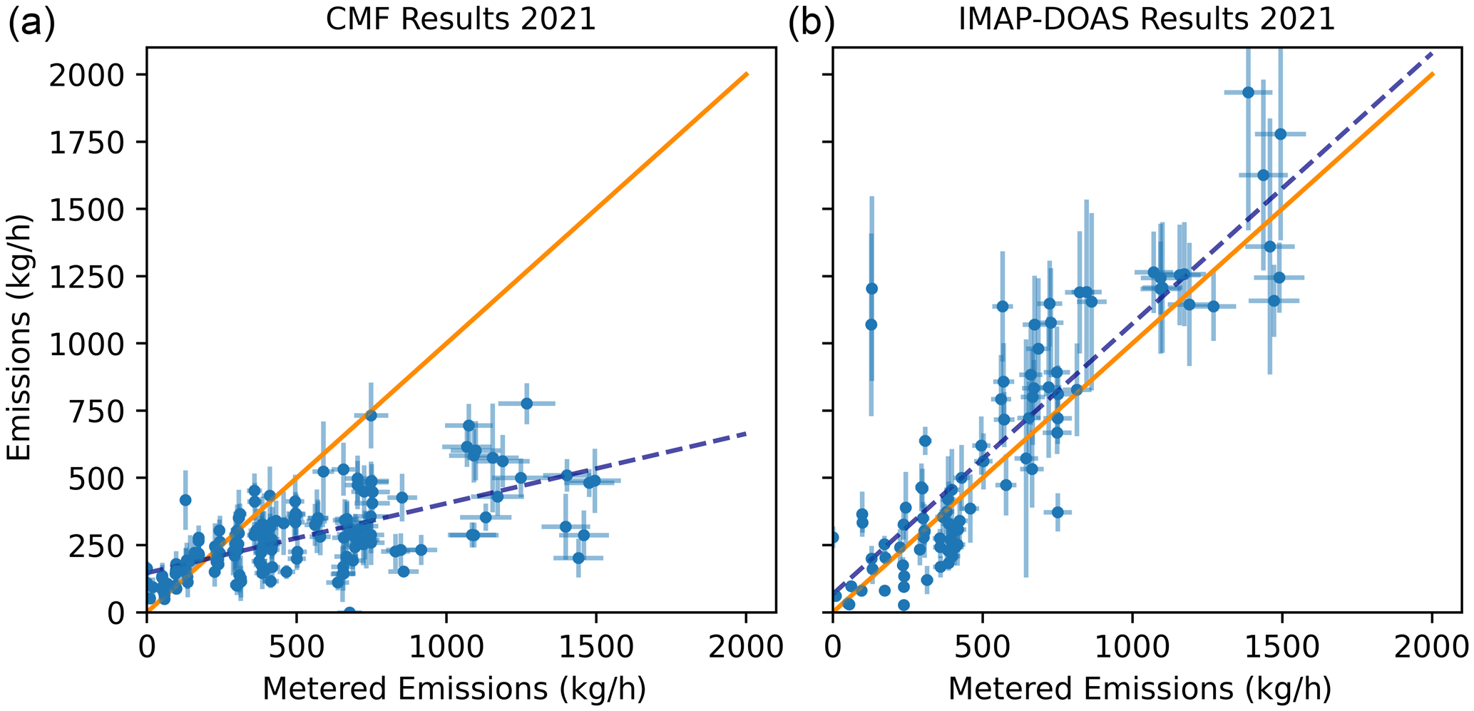
Figure 1 CMF (a) and IMAP-DOAS (b) comparison to metered emission rates for the 2021 controlled-release experiment with shorter-than-normal flight lines. An ordinary least squares (OLS) fit to CMF results in $y=\mathrm{0.26}x+\mathrm{146}$ with R² = 0.42. An OLS fit to IMAP-DOAS results in $y=\mathrm{0.98}x+\mathrm{83}$ with R² = 0. 72. For both panels, the solid line represents the 1 : 1 line, the dashed line is the OLS fit, and the error bars represent 1σ uncertainties.

The bias seen in the 2021 CMF result prompted us to revisit the line length assumption described above (i.e., the line length pixel minimum must be 7 times the length of active bands). A review of our standard line lengths for field campaigns, specifically the larger regional surveys of the Permian basin performed between 2019 and 2021 (Cusworth et al., 2019, 2022), revealed that the line lengths flown during the 2021 controlled-release experiment were an order of magnitude shorter than normal operations (Fig. 2). In the CMF formulation (Eq. 1), the magnitude of a CH₄ enhancement is directly related to the mean and covariance of pixels contained in a column. With a smaller flight line, the column covariance is calculated with a smaller number of pixels; this means that pixels with a CH₄ enhancement have a larger influence over the covariance, thereby making any deviations from the background (i.e., CH₄ enhancements) possibly smaller. The systematic low bias seen in Fig. 1a from the CMF result could therefore be indicative of flight lines that were systematically too short. In contrast, as IMAP-DOAS is a pixel-based algorithm and is therefore indifferent to flight lines lengths for quantification, the much closer agreement to metered emission rates in Fig. 1b is additional evidence that short flight lines drove much of the bias in the CMF result.

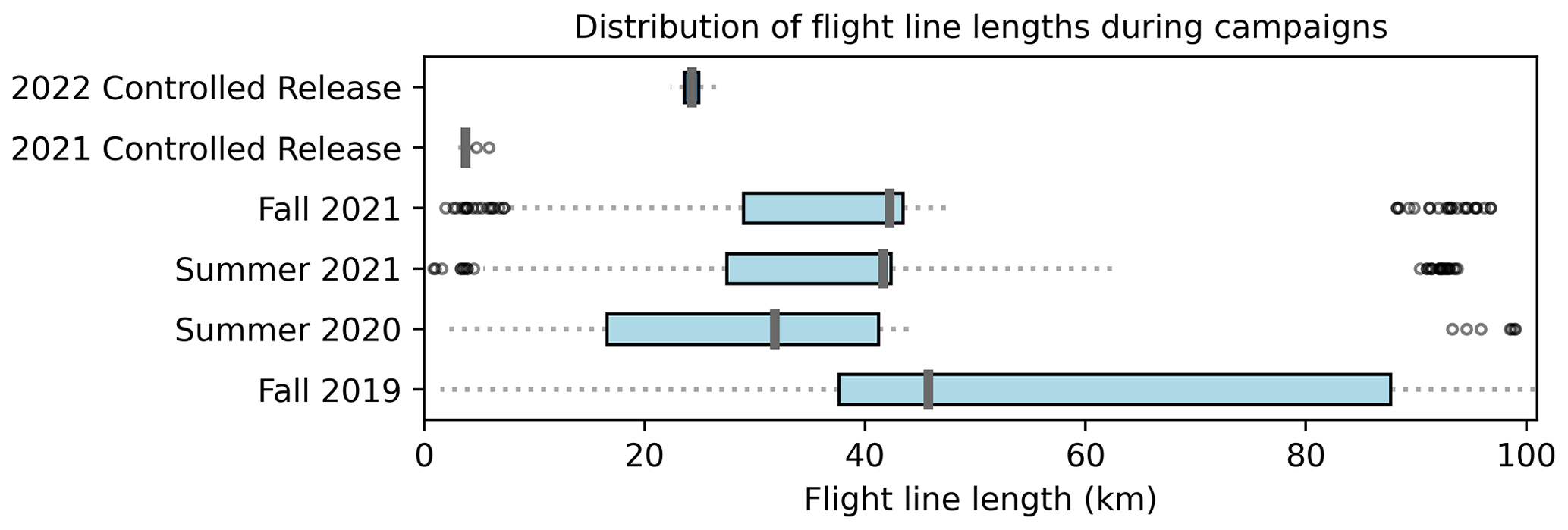
Figure 2 Flight line lengths during the 2021 and 2022 controlled-release experiments compared to Carbon Mapper Permian field campaigns (Cusworth et al., 2021, 2022). The data are displayed as a box plot, with the blue box representing the interquartile range, the gray bar representing the median, the dashed lines representing the respective minimum and maximum, and the black circles representing outliers.

To provide further evidence that systematically short flight lines bias CMF-derived concentrations (and therefore emissions), we selected a subset of 50 flight lines that were flown during standard campaign operations in the Permian between 2019 and 2021. We isolated a single unique plume in each line, cropped the scene around that plume such that it was 1200 pixels (or 6 km) in the along-track direction, and then ran the CMF algorithm. As the 2019–2021 Permian campaigns were flown at higher altitudes (5–9 km), we cropped these scenes to match the average number of pixels per column during the 2021 controlled-release experiment. Therefore, these cropped scenes are representative of the statistical sampling conditions also present in the controlled-release CMF results. Figure 3 shows the results of cropping 2019–2021 Permian scenes to the same pixel dimension as the 2021 controlled-release experiment. What is immediately obvious is that estimated emissions from these cropped scenes are much lower than the standard CMF emission estimates that use all pixels in the along-track direction. An OLS fit between the cropped and standard CMF emissions results in $y=\mathrm{0.14}x+\mathrm{81}$ with R²=0.47, showing a severe reduction in estimated emissions. This lends additional evidence that the poor results in Fig. 1 were driven primarily by short flight lines.

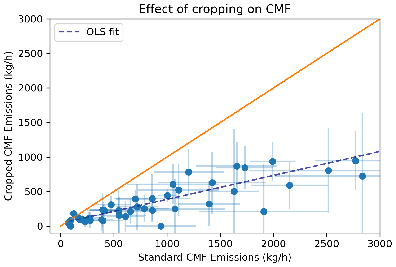
Figure 3 Effect of cropping scene length on CMF results. Scenes were taken from 2019–2021 Permian campaigns that were flown under normal operations (i.e., not a controlled release experiment) and then cropped to 1200 pixels in length; following this, the CMF was rerun. The resulting emissions are compared to the emissions from the standard full-line CMF processing. The OLS fit results in $y=\mathrm{0.35}x+\mathrm{40}$ with R² = 0.77.

The analyses described by Figs. 1, 2, and 3 lend confidence that the 2021 bias in CMF results was driven by short flight lines. However, this unfortunately renders the 2021 controlled-release experiment incapable of assessing how a properly constrained (i.e., 20–50 km flight line length) CMF algorithm performs quantitatively against a standard metered emission rate. Nevertheless, given the good performance of IMAP-DOAS on the 2021 controlled-release data, we cross-compared emission rates from the 2019–2021 Permian campaigns derived from both CMF and IMAP-DOAS algorithms. This subset includes more than 60 plumes that relate to 20 distinct facilities that were imaged on at least 3 separate days during airborne campaigns by GAO during the Permian 2019–2021 campaigns (Cusworth et al., 2022). These plumes represent a dynamic range of emission rates reported by the CMF algorithm (90–3900 kg h⁻¹) and portray a diversity of infrastructure types in this region. The results of the IMAP-DOAS–CMF comparison are shown in Fig. 4. Figure 4a shows instantaneous plume-to-plume emission comparison for the different retrieval approaches. The data comparison shows general agreement between the two retrieval approaches. An OLS fit results in $y=\mathrm{0.72}x+\mathrm{307}$ with R²=0.67.

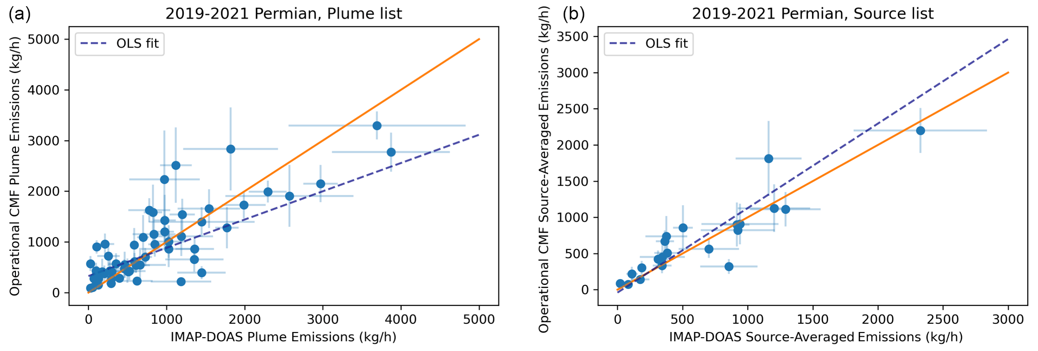
Figure 4 Panel (a) is a comparison of instantaneous emission rates for a subset of 2019–2021 plumes in the Permian Basin between the operational CMF and IMAP-DOAS. Panel (b) is a comparison of CMF and IMAP-DOAS for source-averaged emission rates. Error bars represent 1σ uncertainties in emissions. In panel (a), the OLS regression fit (plume list with instantaneous emissions) is as follows: $y=\mathrm{0.72}x+\mathrm{307}$ with R² = 0.67.

In practice, when summarizing the results from campaigns and constructing emission budgets for regions or facilities, we take persistence-averaged emission rates derived from multiple overpasses of a facility (e.g., the average emission rate over multiple observations; Cusworth et al., 2021). Figure 4b shows the comparison of IMAP-DOAS and CMF after averaging and applying persistence adjustment to the emissions. Here, the comparison between retrieval approaches shows very close correspondence, with an OLS fit of $y=\mathrm{0.89}x+\mathrm{120}$ and R² = 0.82. As expected, the variability in emissions on a plume-by-plume basis gets averaged out in Fig. 4. As the only difference between CMF- and IMAP-DOAS-derived emission rates is the concentration retrievals, the improved correlation between single-realization plumes in Fig. 4a and multiple-realization sources in Fig. 4b shows that much of the retrieval uncertainty from these two approaches is unbiased because they begin to converge in agreement with additional sampling.

3.2 Column matched filter sensitivity tests

The results in Figs. 1 and 3 provide evidence that a reduced flight line length hampers the CMF's quantitative performance; however, the results do not reveal what the appropriate line length is to ensure good quantification. In order to improve results for the 2022 controlled release and to ensure that we are able to accurately quantify plumes operationally, we performed an analysis to determine the minimum line length for good quantification. To do this we identified eight sources that had at least three flyovers from GAO and were located in long lines. This resulted in 24 individual scenes to analyze. These scenes ranged from 125 to 27 km in length. Using the full flight line lengths, the plumes within each scene have CMF-derived emission rates between 70.7 and 3980 kg h⁻¹. Scenes were acquired from various campaigns, including the Permian 2021, Denver-Julesburg summer 2021, North East 2021, California summer 2020, and Permian fall 2021 (Thorpe et al., 2023; Cusworth et al., 2022).

Each scene was cropped to 2000 pixels (6–10 km) centered on the identified plume. This crop was then iteratively increased in 1000-pixel (3–5 km) increments until the full scene length was reached. This produced between 6 and 24 cropped images per scene. Each scene crop was processed through the CMF and an IME algorithm. We used IME over emission rates because the IME isolated changes in the CH₄ retrieval better than a full emission estimate. Additional details on the methods used in this analysis can be found in Sect. S3 in the Supplement.

We found that, in general, the IME increases as the pixel count in each column increases; however, the rate of increase decreases with pixel count. While not asymptotic, the small increase in the IME after a certain threshold likely means that there is an optimal point (or distance) that is sufficient for quantifying an emission rate. Figure 5a shows the pixel count vs. the IME for three different images of one CH₄ plume. The IME increases rapidly at the low pixel counts (short lines) and then levels off as the line gets longer. We determined this optimal point by calculating the “knee” in the curve (or the point where the change in IME is minimal compared with the change in the scene length). We found that, for all the plumes assessed, the median knee was 7000 pixels (or about 21 km when the aircraft is flown as 3 km). We compared the IME from the 7000 pixels to the standard scene length IME and found generally good agreement (Fig. 5b). From this, we can also conclude that the minimum line length needed to produce a good quantification with the CMF is about 21 km. This minimum line length is well within the lengths flown from previous Permian surveys (Fig. 2).

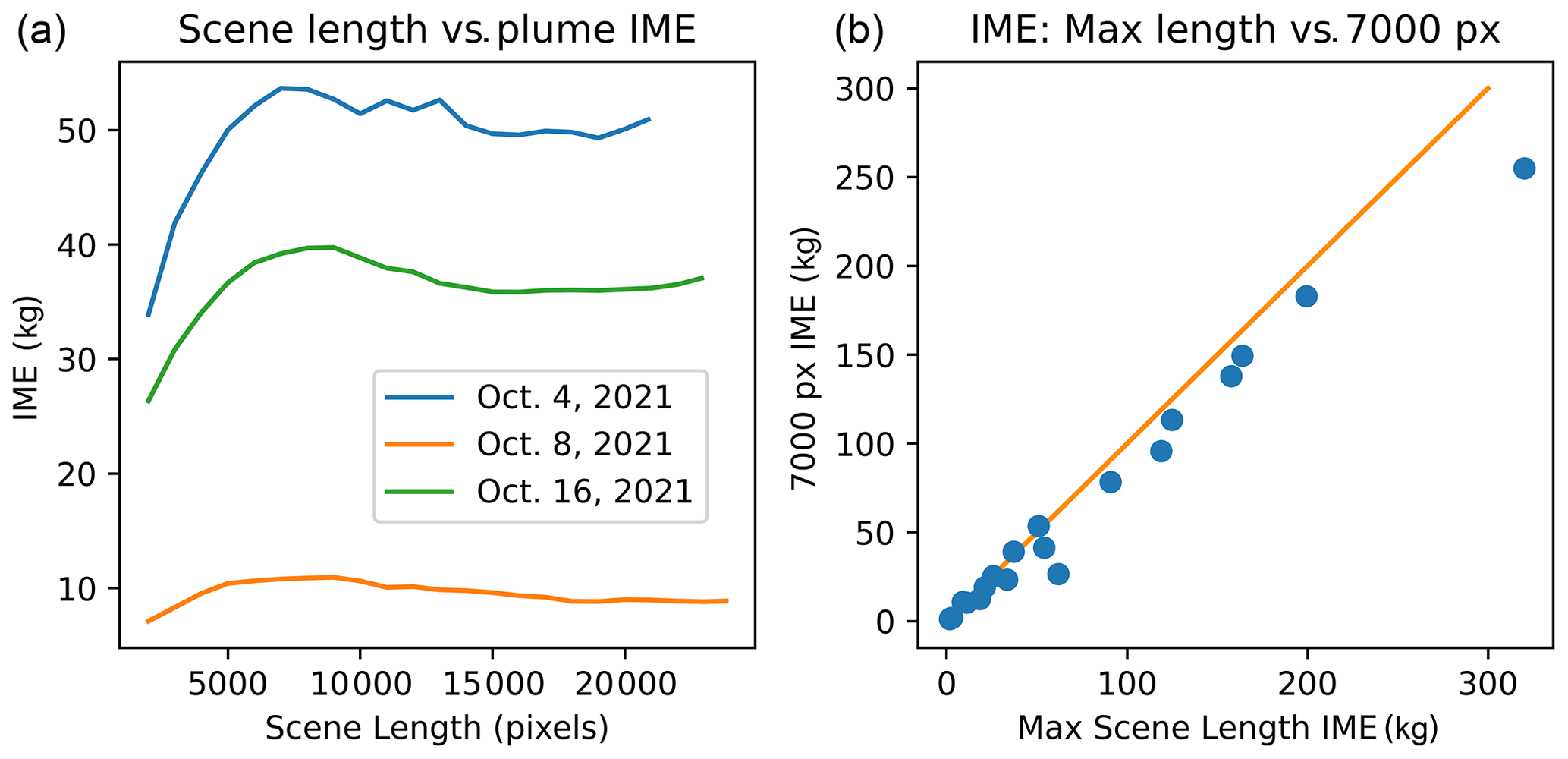
Figure 5 Panel (a) shows the scene length (pixels) vs. the IME from the matched filter for three plumes from a campaign in October 2021. Panel (b) shows the comparison of calculated emission rate plumes with a scene length of 7000 pixels (or 21 km when the aircraft is flown at 3 km) compared to the calculated emission rate for the full scene length (length variable depending on scene). The agreement is good, indicating that a ∼ 20 km line is a sufficient length for good quantification.

3.3 The 2022 controlled release

The results in Fig. 5 prompted us to require a minimum flight line distance of 20 km during the 2022 controlled-release experiment. The estimated airborne emission rates compared to metered emissions for the 2022 controlled release are shown in Fig. 6 for both CMF and IMAP-DOAS. The OLS fit between the CMF results and the metered emissions results in $y=\mathrm{0.90}x+\mathrm{42}$ and R²=0.88. The OLS fit between IMAP-DOAS and metered emissions results in $y=\mathrm{1.14}x-\mathrm{19}$ and R² = 0.81. These values differ slightly from the values published in El Abbadi et al. (2023) due to different quality filters, but the trends remain the same. The results of the CMF are much improved from the 2021 controlled release. These results further highlight the need for appropriately long flight lines. The improved results provide additional assurance that previous airborne campaigns, most of which have flight lines longer than 20 km, do not have a systematic underestimate.

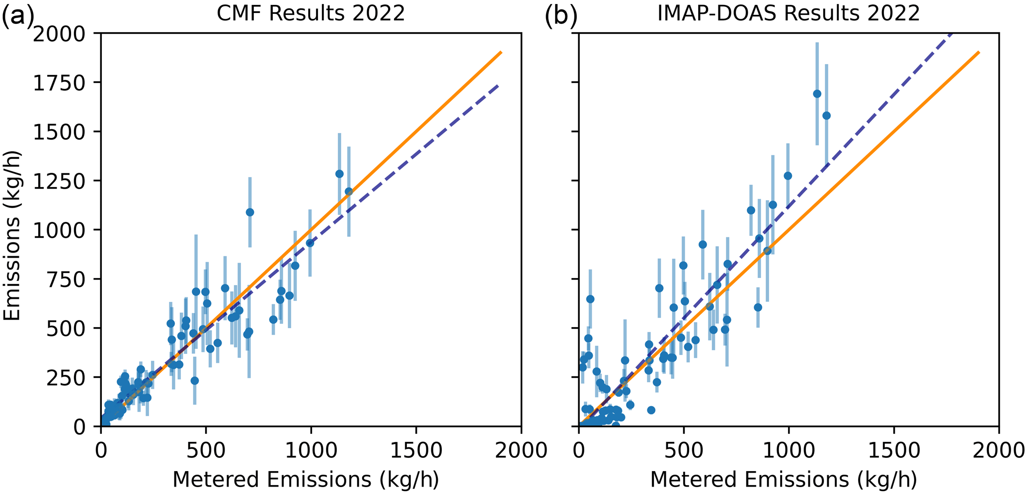
Figure 6 CMF and IMAP-DOAS comparison to metered emission rates for the 2022 controlled-release experiment. An OLS fit to CMF results in $y=\mathrm{0.90}x+\mathrm{42}$ with R² = 0.88. An OLS fit to IMAP-DOAS results in $y=\mathrm{1.14}x-\mathrm{19}$ with R² = 0.81. For both panels, the solid line represents the 1 : 1 line and the dashed line is the OLS fit. The error bars represent 1σ uncertainties; there is error present on the x axis, but the error is too small to visualize.

The CMF and IMAP-DOAS produced comparable results for the 2022 experiment, similar to the results seen from Permian campaigns shown in Fig. 4. However, other features exist that may corrupt a CMF result, even for long flight lines that were not explicitly tested during the 2022 controlled-release experiment. For example, flares or specular reflections from solar panels often result in saturated or atypical backscattered radiance spectra. If these spectra are observed anywhere in a column and not removed, they can enter into a covariance calculation, causing the CMF results in that column to be biased. In addition, the presence of too many dark pixels, like a waterbody, can also negatively affect the CMF. Although not affected by other pixels, physics-based retrievals like IMAP-DOAS are also prone to retrieval artifacts for complicated pixels. Therefore, controlled-release tests across a host of simple to complex observing environments will further refine algorithms to quantify concentrations and emissions.

3.4 Detection limits

Although biased by short flight lines, the CMF results from the 2021 controlled-release experiment performed well with respect to CH₄ plume detection. The CMF ability to detect emissions has proven insensitive to line length, but these detection limits are strongly influenced by other observing conditions. To determine detection limits, we used logistic regression to build detection models. For the first set of models (Fig. 7a), we only used the metered emission rates as the predictor variable and built separate models for the 2021 and 2022 experiments. This allows us to compare the detection limits under two different observing conditions. We also made a more general model (Fig. 7b); for this, we combined both experiments and used wind speed as well as the metered emission rates as predictor variables. Other factors like solar zenith angle (SZA) and albedo should also be used as predictor variables; however, for these experiments, there was not enough variability in albedo to use it as a predictor variable, and the SZA, in this case driven by time of day, was also correlated with the metered release rates and was, therefore, not used as a predictor variable.

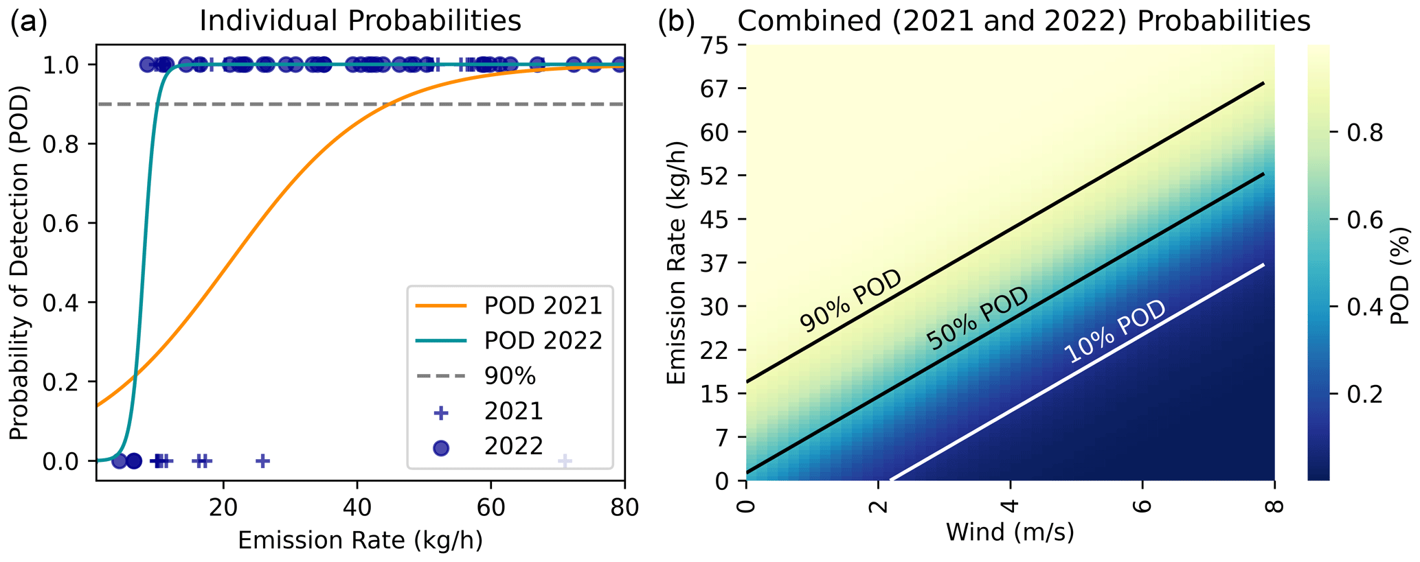
Figure 7 Probability of detection (POD) for the AVIRIS-NG/GAO instrument using the CMF methane retrieval algorithm. Panel (a) shows the individual POD curves for the 2021 and 2022 controlled release. The points at zero represent null detections and the points at one represent positive detections. Panel (b) shows the combined POD contours and includes wind.

In the 2022 controlled-release experiment, the smallest plume detected was 8.6 kg h⁻¹ and the 90 % probability of detection (POD) was 10 kg h⁻¹. However, these were ideal conditions. The albedo was 42 % in the area surrounding the controlled-release site, which is considered high, and the wind speeds were low (mean of 1.78 m s⁻¹). Typical operating conditions are more challenging, which can lead to higher minimum detection limits. The 2021 controlled release had more challenging conditions: the wind speeds were higher (mean of 2.5 m s⁻¹), although not extreme, and the surface albedo was 24.5 % and also more varied. In the 2021 experiment, the smallest plume detected was 9.8 kg h⁻¹ and the 90 % POD was 45 kg h⁻¹. It is important to note that the smallest release rate was also 9.8 kg h⁻¹; thus, for 2021, there are no data for releases below this value, and our understanding of detection below 9.8 kg h⁻¹ is consequently incomplete. When we combine both controlled-release experiments and add wind as a predictor variable, we can more clearly visualize how detection limits can change depending on the conditions. The 90 % POD ranges from 17 to 68 kg h⁻¹ as a function of wind speed (Fig. 7). These results are consistent with previous controlled-release results and with other analyses of POD curves that showed an AVIRIS-NG 90 % POD of 16–33 kg h⁻¹ (Thorpe et al., 2016; Conrad et al., 2023). The POD is also a function of albedo and SZA, but these controlled-release experiments were not designed to test and isolate those parameters. In practice, we anticipate the POD performance to vary across observing regions and seasons (Gorroño et al., 2023). Specifying and understanding observing conditions is critical to interpreting POD and minimum detection results.

4 Conclusion

The nonstandard short flight lines flown during the 2021 controlled-release experiment resulted in an unexpected low bias in CMF-retrieved CH₄ concentrations which propagated into low emission rates. Here, we tested that hypothesis by applying the pixel-wise IMAP-DOAS retrieval to the 2021 controlled-release results. We found a much improved result, with IMAP-DOAS-derived emission rates showing strong correlation and little bias across the experiment. We subsequently flew longer, more representative flight lines in the 2022 controlled-release experiment and eliminated bias in both the CMF and IMAP-DOAS retrievals. Both experiments were used to assess the minimum detection limit as well as the 90 % POD. These experiments highlighted the importance of observing conditions when evaluating the POD.

Here, we also highlight the various strength and weaknesses of the two main retrieval algorithms. The CMF is a fast and reliable detection algorithm but is sensitive to scene dynamics, specifically scene length, for quantification. Here, we show that the 2021 controlled release did not meet the scene length requirements for good quantification, but we also show that most Carbon Mapper flight lines meet the scene length requirement and produce good quantitative results. IMAP-DOAS, on the other hand, is too slow to run as a detection algorithm, but it can produce more reliable quantification estimates and does not rely on other aspects of a scene. However, continuing work is needed to robustly quantify background concentrations over a diverse set of observing conditions. Ideally, these two algorithms can be used in tandem: the CMF for rapid detection and IMAP-DOAS after for a robust quantification.

As we move towards routine and global monitoring with remote sensing, these results provide confidence in our ability to accurately quantify CH₄ emissions. These results also highlight the importance of controlled-release testing in order to assess and understand retrieval algorithms. As a larger constellation of instruments are used to map CH₄ (Jacob et al., 2022), more controlled-release tests will be needed to fully validate emissions.