the Creative Commons Attribution 4.0 License.
the Creative Commons Attribution 4.0 License.
 | 08 Feb 2023
Estimation of raindrop size distribution and rain rate with infrared surveillance camera in dark conditions
Jinwook Lee
Jongyun Byun
Jongjin Baik
Changhyun Jun
This study estimated raindrop size distribution (DSD) and rainfall intensity with an infrared surveillance camera in dark conditions. Accordingly, rain streaks were extracted using a k-nearest-neighbor (KNN)-based algorithm. The rainfall intensity was estimated using DSD based on a physical optics analysis. The estimated DSD was verified using a disdrometer for the two rainfall events. The results are summarized as follows. First, a KNN-based algorithm can accurately recognize rain streaks from complex backgrounds captured by the camera. Second, the number concentration of raindrops obtained through closed-circuit television (CCTV) images had values between 100 and 1000 mm−1 m−3, and the root mean square error (RMSE) for the number concentration by CCTV and PARticle SIze and VELocity (PARSIVEL) was 72.3 and 131.6 mm−1 m−3 in the 0.5 to 1.5 mm section. Third, the maximum raindrop diameter and the number concentration of 1 mm or less produced similar results during the period with a high ratio of diameters of 3 mm or less. Finally, after comparing with the 15 min cumulative PARSIVEL rain rate, the mean absolute percent error (MAPE) was 49 % and 23 %, respectively. In addition, the differences according to rain rate are that the MAPE was 36 % at a rain rate of less than 2 mm h−1 and 80 % at a rate above 2 mm h−1. Also, when the rain rate was greater than 5 mm h−1, MAPE was 33 %. We confirmed the possibility of estimating an image-based DSD and rain rate obtained based on low-cost equipment during dark conditions.
- Article
(6571 KB) - Full-text XML
- BibTeX
- EndNote


Precipitation data are vital in water resource management, hydrological research, and global change analysis. The primary means of measuring precipitation is to use a rain gauge (Allamano et al., 2015) to collect raindrops from the ground level. Due to the restrictions in the installation environment of the rain gauge, it can be difficult to understand the spatial rainfall distribution in mountains and urban areas (Kidd et al., 2017). Furthermore, the tipping-bucket-type rain gauge, which accounts for most rain gauges, has a discrete observation resolution (0.1 or 0.5 mm) for the discrete time steps, producing uncertainty in temporal rainfall variation. For this reason, weighing gauges are used very often nowadays instead of the tipping bucket type. The weighing gauge is a meteorological instrument used to observe and analyze various precipitation, including rainfall and snowfall. Also, the tipping bucket has a large error due to the observation time delay when the rainfall is less than 10 mm h−1 compared to the weighing gauge. However, when the observation time size is set to 10 to 15 min, then the relative percentage error has a very low value of −6.7 % to 2.5 %, resulting in high accuracy (Colli et al., 2014).
In contrast, it is possible to obtain spatial rainfall information on a global scale with remote sensing techniques (Famiglietti et al., 2015). However, remote sensing techniques provide only indirect measurements that must be continuously calibrated and verified through ground-level precipitation measurements (Michaelides et al., 2009). Recently, a disdrometer capable of investigating the microphysics characteristics of rainfall has been used for observation instead of the traditional rainfall observation instrument (Kathiravelu et al., 2016). However, these devices cannot be widely installed because of their high cost and the difficulty in accessing observational data. Consequently, a high-resolution and low-cost ground precipitation monitoring network has not yet been established.
With the advent of the Internet of Things (IoT) era, using non-traditional sources is attractive for improving the spatiotemporal scale of existing observation networks (McCabe et al., 2017). In recent years, such cases have been common in rainfall observation. For example, there have been attempts to estimate rainfall using sensors to capture signal attenuation characteristics in commercial cellular communication networks (Overeem et al., 2016), vehicle wipers (Raibei et al., 2013), and smartphones (Guo et al., 2019). Furthermore, crowdsourcing information has been used to confirm the utility of estimating regional rainfall (Haberlandt and Sester, 2010; Rabiei et al., 2016; Yang and Ng, 2017).
In a similar context, a surveillance camera is a sensor with high potential. Surveillance cameras are often referred to as closed-circuit television (CCTV). Compared with other crowdsourcing methods, the visualization data of surveillance cameras are highly intuitive (Guo et al., 2017). Therefore, they have been used in various fields (Cai et al., 2017; Nottle et al., 2017; Hua, 2018). In South Korea, public surveillance camera installations have been rapidly increasing, from approximately 150 000 in 2008 to 1.34×10⁶ in 2020 – approximately a public CCTV camera per 0.07 km2. Thus, the potential for precipitation estimation using camera sensing is expected to be greater in South Korea.
Recently, various studies have been conducted to estimate rainfall intensity using the rain streak image obtained from surveillance camera videos. Many studies attempted to use artificial intelligence to capture changes in the image captured by the camera when it rains (Zen et al., 2019; Avanzato and Beritelli, 2020; Wang et al., 2022). In contrast, some studies have tried to estimate rainfall intensity using geometrical optics and photographic analyses. Typically, the rain streak layer is separated from the raw image or video. A rain streak is the visual appearance of raindrops caused by visual persistence – raindrops falling because of the blur phenomenon of raindrop movement from the camera's exposure time appear as streaks on the image. Garg and Nayar (2007) made one of the first attempts to measure this rainfall.
These previous studies indeed confirmed the possibility of rainfall measurement using surveillance cameras. However, several limitations still prevent the actual expansion of the measurement systems using surveillance cameras. In general, most surveillance cameras are installed for monitoring purposes, and people's faces are inevitably captured. Therefore, it is not easy to disclose the data due to privacy concerns. Data storage and transmission are also limitations. Since most surveillance cameras use a hard disk, the data must be extracted directly. In other words, rainfall estimation cannot be done in real time unless a system is in place to transmit data over the internet. In addition, the applicability to nighttime is more limited. In the case of general surveillance cameras in the past, observation is possible only when sunlight exists. For the observation system to expand, these various limitations must be addressed, and it seems that a lot of time and effort are needed. Nevertheless, research to develop algorithms using surveillance cameras in various conditions and to confirm applicability can have sufficient meaning. The case of dark conditions is one of the conditions worth studying. This is because the recently installed surveillance cameras are equipped with an infrared (IR) recording function, so most cameras will be able to take videos at night soon. However, the final purpose of utilizing these devices and the method is not to replace existing devices. It could be a supplement to improve the spatiotemporal resolution and accuracy of existing observation instruments. In particular, a study on the drop size distribution of rainfall, rather than simple rainfall estimation, would have more potential application value.
Since then, many studies have been conducted to develop and improve efficient algorithms. Allamano et al. (2015) proposed a framework to estimate the quantitative rainfall intensity using camera images based on physical optics from a hydrological perspective. Dong et al. (2017) proposed a more robust approach to identifying raindrops and estimating rainfall using a grayscale function, making grayscale subtraction nonlinear. Jiang et al. (2019) proposed an algorithm that decomposes rain-containing images into rain streak layers and rainless background layers using convex optimization algorithms and estimates instantaneous rainfall intensity through geometric optical analysis.
Some studies (e.g., Dong et al., 2017) have sought to estimate the raindrop size distribution (DSD) using a surveillance camera. However, the existing studies have focused on times when a video can be captured with visible light. It is impossible to obtain input data without visible light using the existing image-based rainfall measurement method. Thus, these methodologies are only applicable in daytime conditions. However, when recording using infrared rays, it is possible to obtain a rainfall image even when there is no sunlight. No study has estimated the rain in dark conditions, to our knowledge. Furthermore, most previous studies did not verify the estimated DSD using a disdrometer. In contrast, this study estimated DSD with an infrared surveillance camera in dark conditions, the basis on which rainfall intensity was also estimated. Rain streaks were extracted using a k-nearest neighbor (KNN)-based algorithm. The DSD was used to calculate rainfall intensity with physical optics analysis and verified using a PARticle SIze and VELocity (PARSIVEL) disdrometer (Löffler-Mang and Joss, 2000).
2.1 Recording video containing rain streaks using an infrared surveillance camera
The surveillance camera records video. The video looks continuous, but it is also composed of discrete still images or so-called frames. The frequency of recording frames (i.e., acquisition rate) is called frame per second (fps). In other words, fps is how many images are taken per second when recording a video. Another important factor in video recording is exposure time. Exposure time, also called shutter speed, refers to the time the camera sensor is exposed to light to capture a single frame. The real raindrops are close to a circle, but in a single image, the raindrops look like a streak. This is because raindrops move at a high speed during the exposure time. Therefore, the raindrops that moved during the exposure time are visualized in the rain streaks in a single frame.
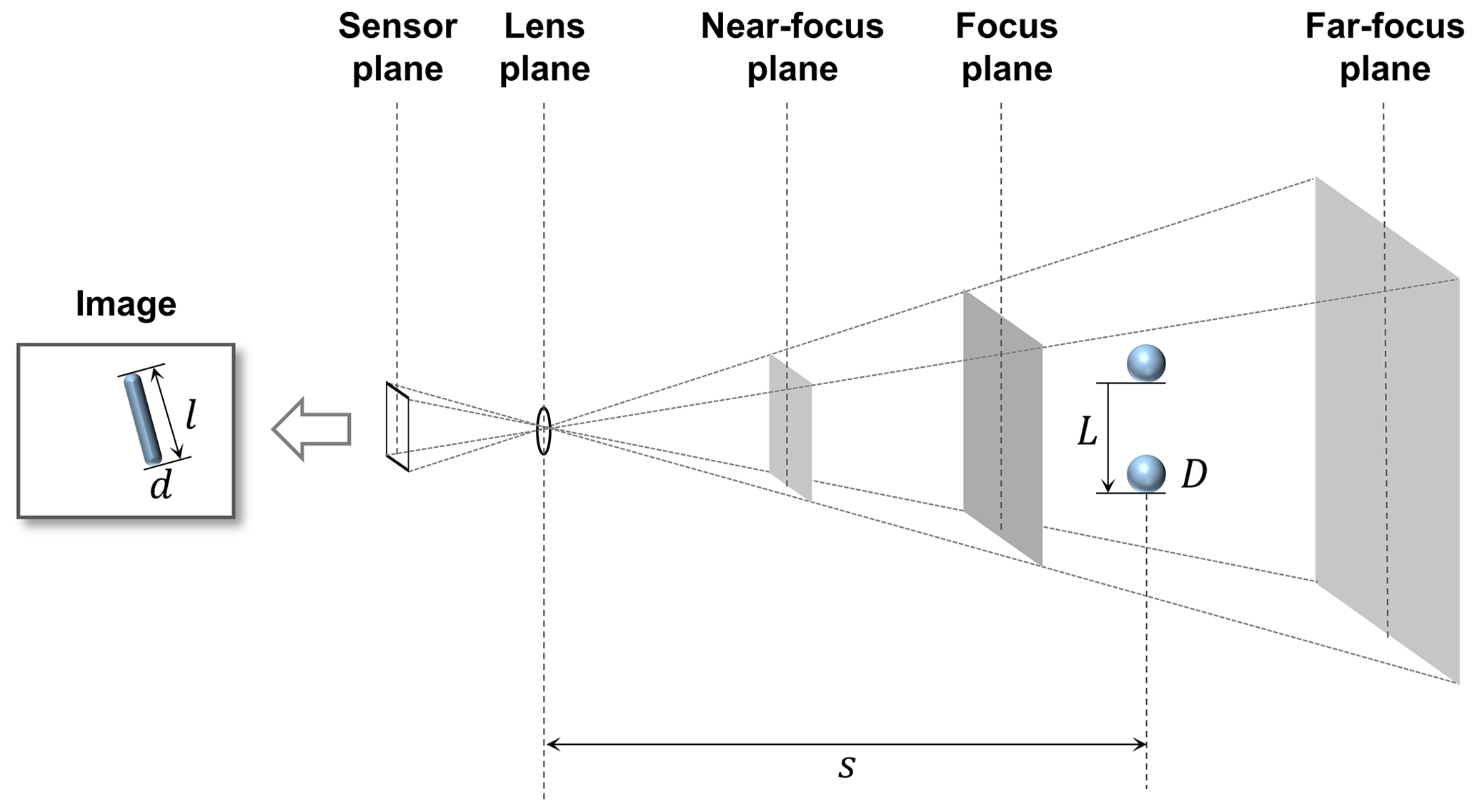
Figure 1Schematic diagram of the photographed rain streak in the image and the movement of a raindrop during the exposure time.
Figure 1 shows an example of capturing a raindrop for a single frame. Here, only the raindrops near the point of focus are visible, and objects that are more than a certain distance appear invisible. That is, the point at which the focus is best is called the focus plane, and there is a range in which it can be recognized that objects are focused before and after the focus plane. The closest plane that can be considered to be in focus is called the near-focus plane, and the farthest plane is called the far-focus plane. This range is generally called depth of field (DoF). Ultimately, the rainfall intensity can be estimated based on the volume and raindrops in the DoF.
In this study, an infrared surveillance camera was considered under dark conditions. Here, the dark condition refers to a condition in which raindrops cannot be captured by a general surveillance camera with visible light. Infrared cameras emit near-infrared rays through an infrared emitter and receive the reflected light from the objects. Accordingly, it has the advantage of being able to detect raindrops that are invisible to the human eye.
2.2 Algorithm for identifying rain streaks and estimating DSD and rain rate
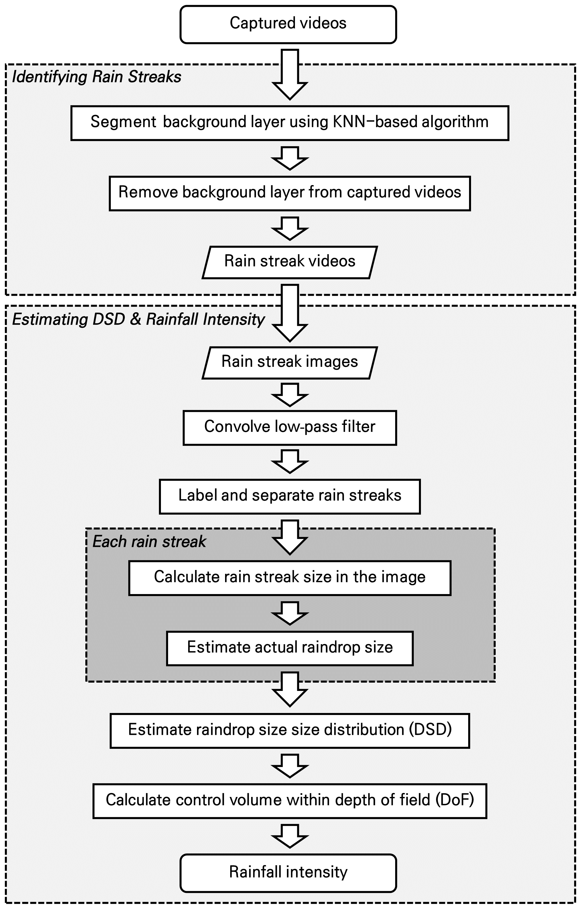
Image-based rainfall estimation can be divided into two processes, i.e., identifying rainfall streaks and estimating DSD. Figure 2 illustrates these processes in a flowchart. Identifying rain streaks requires an algorithm that separates the moving rain streaks from the background layer. Next, in estimating DSD, raindrops are extracted from the image of the rain streaks, and the overall distribution is obtained.
Most existing algorithms aim to remove raindrops in images because raindrops are considered noise in object detection and tracking (Duthon et al., 2018). Such algorithms are categorized into multiple-image-based and single-image-based approaches (Jiang et al., 2018).
For example, Garg and Nayar (2007) classified the conditions in which the brightness difference between the previous pixel and that of the next pixel exceeds a specific threshold over time, assuming that the background is fixed. Improved algorithms were then developed, considering the temporal correlation of raindrops (Kim et al., 2015) and chromatic properties (Santhaseelan and Asari, 2015). Tripathi and Mukhopadhyay (2014) proposed a framework to remove rain that reduces the visibility of the scene to improve the detection performance of image feature information. However, single-image-based algorithms rely more on the properties of raindrops (Deng et al., 2018). The central idea of a single-image-based algorithm is to decompose rain-containing images into rainless layers (Li et al., 2016; Deng et al., 2018; Jiang et al., 2018).
An image including grayscale rainfall may be mathematically expressed in a two-dimensional (2D) matrix in which each element has a grayscale value. A single image (m×n) is expressed as follows (Jiang et al., 2018):
where , , and are the raw image, rain-free background layer, and rain streak layer.
Accordingly, various algorithms are available for rain streak identification. Different still image and video-based algorithms have been proposed to eliminate objects such as moving objects for application to actual surveillance cameras. However, most of these algorithms face optimization problems because of the vast number of decision variables (Jiang et al., 2019). This task is not easy to solve or requires excessive computation time. Therefore, existing studies present techniques suitable for post-analysis rather than application in real time. The use of complex algorithms can increase versatility and accuracy, but there is a tradeoff that reduces computational speed. The time required for such computing is a critical disadvantage in practical applications for estimating rainfall intensity.
In this study, a KNN-based segmentation algorithm (Zivkovic and van der Heijden, 2006), a popular non-parametrical method for background subtraction, was considered for segmenting the rain streaks (foreground) and background layers. KNN is used in classification and regression problems (Bouwmans et al., 2010). The concept of KNN is that similar things are close – the KNN-based segmentation algorithm finds the closest k samples (neighbors) to the unknown sample by using the Euclidean distance to determine the class (i.e., foreground or background). Thus, the KNN-based segmentation method to detect foreground changes in the video was used to identify rain streaks by recording infrared videos under conditions with little background influence. In the algorithm, The KNN subtractor works by updating the parameters of a Gaussian mixture model for more accurate kernel density estimation (Trnovszký et al., 2017). KNN is more efficient for local density estimation (Qasim et al., 2021); therefore, the algorithm is highly efficient if the number of foreground pixels is low.
Table 1Parameters in KNN background subtractor package in OpenCV.
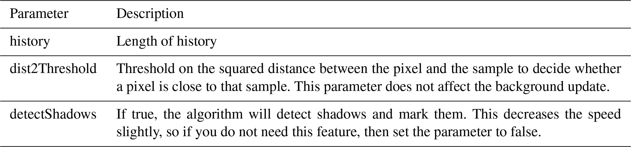
We used the package provided by OpenCV to implement the KNN-based segmentation algorithm (Zivkovic and van der Heijden, 2006). Accordingly, three main parameters (history, dist2Threshold, detectShadows) needed to be set. Table 1 presents the description of the parameters used for the KNN background subtractor package.
It is essential to capture raindrops within the camera's depth of field (DoF) to calculate the final DSD and rainfall intensity. Accordingly, this study proposed a novel algorithm to extract each rain streak from the rain streaks image. First, we applied a low-pass filter to the rain streaks image to remove unfocused raindrops that may remain in the image, which smooths each pixel using a 2D kernel. Videos from infrared mode have usually a blur effect. Thus, the additional 2D kernel was applied to remove the pixels having blur. Highly detailed parts (e.g., out-of-focus raindrops and some noises) are erased, leaving some clear rain streaks. A background layer with a value of 0 and a part not in the image was separated to extract the rain streaks and labeled one by one to identify each rain streak from the image.
Because the rain streak observed in the surveillance camera image causes an angle difference (influenced by the wind), a diameter estimation process considering the angle of the rain streak (fall angle of a raindrop) is required. If the angle of the rain streak is considered and converted to the raindrop diameter through the horizontal pixel size in the image, then the shape change in the raindrop because of air buoyancy (i.e., during the falling of the raindrop) may not be reflected, and overestimation can occur.
Accordingly, the representative angle of each extracted rain streak was calculated. The border information of each rain streak was obtained, and the center axis information of the rain streak was obtained based on the border information used to calculate the drop angle. Moreover, the rain streak was rotated to set the long and short axes of the streak at 0 and 90∘, using the angle information.
The size of raindrops in the rain streaks image can be estimated through the analysis of microphysical characteristics of the raindrop and geometric optical analysis (Keating, 2002). The instantaneous velocity of a raindrop on the ground can be estimated from the exposure time and the size of the raindrop. However, the distance from the raindrop to the lens surface (i.e., the object distance) is unknown and should be inferred. Object distance can be calculated through physical optics analysis because it causes perspective distortion. Assuming a raindrop is spherical, the length of the trajectory where the raindrop falls when the camera is exposed and the diameter of the raindrop can be inferred through the lens equation as follows (Keating, 2002):
where s is the distance from the raindrop to the lens plane (mm). L(s) and D(s) are the length of falling trajectory during camera exposure (rain streak) and the raindrop's diameter. df is the focus distance (mm), and f is the focal length (mm). hs and ws are the vertical and horizontal sizes of the active area of the image sensor (mm), and hp and wp are the vertical and horizontal sizes of the captured image (in the number of pixels). lp and dp are the length and width of the rain streaks in the image (in the number of pixels).
It is then possible to infer the falling speed of raindrops, using the camera's exposure time (Jiang et al., 2019), as follows:
where τ is the exposure time of the camera (seconds), and v(s) is the fall velocity of the raindrop from the image. Furthermore, the fall velocity of a raindrop can be approximated by an empirical formula for raindrop diameter. The most frequently used equation is as follows (Atlas et al., 1973; Friedrich et al., 2013):
where D is the raindrop diameter, and v is the fall velocity of the raindrop. The actual diameter of raindrops can be obtained by solving the equation with the fall velocity obtained through the exposure time and Eqs. (4) and (5). Furthermore, the DoF for the images using the camera's settings information can be calculated, and the effective volume for estimating the rainfall intensity can be obtained. Details of the process are described in previous studies (Allamano et al., 2015; Jiang et al., 2019).
The control volume must be determined to estimate the rainfall intensity using the diameter of each raindrop. An understanding of DoF is required to achieve the volume. The DoF is simply the range at which the camera can accurately focus and capture the raindrops. Calculating this range requires obtaining the near- and far-focus planes as follows:
where sn and sf are the distances from the near- and far-focus planes. cp is the maximum permissible circle of confusion, a constant determined by the camera manufacturers. N is the F number of the lens relevant to the aperture diameter. Accordingly, the theoretical sampling volume (V; m3) indicates the truncated rectangular pyramid between the near- and far-focus planes:
Then, we used the gamma distribution equation, Eq. (6), proposed by Ulbrich (1983), to calculate DSD parameters using data at every 1 min interval.
where N(D) (mm−1 m−3) is the number concentration value per unit volume for each size channel, and N0 (mm m−3) is an intercept parameter representing the number concentration when the diameter has 0 value. D (mm) and Λ (mm−1) are the drop diameter and slope parameter. Raindrops smaller than 8.0 mm were used to avoid considering non-weather data such as leaves and bugs (Friedrich et al., 2013).
The gamma distribution relationship is a function of formulating the number concentration per unit diameter and unit volume. It was proposed by Marshall and Palmer (1948) as an improved model of exponential distribution as a favorable form to reflect various rainfall characteristics. By including the term containing μ in the distribution function, the shape of the number concentration distribution for small drops smaller than 1 mm is improved.
As the Λ decreases, the slope of the distribution shape decreases, and the proportion of the large drops increases. Conversely, as the value increases, the distribution slope becomes steeper, and the weight of the large particles decreases. When μ has a large value, the distribution is convex upward, and it has a distribution with a sharp decrease in number concentration at small diameters, whereas, when it has a negative value, the distribution is convex downward with an increase in the concentration of drops smaller than 1 mm. In the gamma distribution, the μ is mainly affected by the difference in concentration of raindrops smaller than 3 mm (Vivekanandan et al., 2004).
Vivekanandan et al. (2004) explained the reason for using the gamma distribution as follows. First, it is sufficient to calculate the rainfall estimation equation using only the first, third, and fourth moments (Eq. 11) (Smith, 2003). Second, the long-term raindrop size distribution has an exponential distribution shape (Yuter and Houze, 1997).
The raindrop size distribution observed from the ground is the result of the microphysical development of raindrops falling from precipitation clouds. The drop size distribution shape is changed during fall by microphysical processes such as collision, merging, and evaporation, and mainly changes in the concentration of drops larger than 7.5 mm and small drops occur. As a result, the drop size distribution observed on the ground mainly follows the gamma distribution shape (Ulbrich, 1983; Tokay and Short, 1996). The gamma distribution relationship should be used to analyze the distribution of raindrops that are actually floating and falling.
Equation (11) indicates a moment expression for the nth order. For example, the second moment is calculated as the product of the square of the diameter of each channel and the number concentration and the diameter of each channel. Each moment value has a different microphysical meaning. Therefore, the gamma distribution including three dependent parameters is more advantageous in reflecting the microphysical characteristics of the precipitation system than the exponential distribution including two dependent parameters. Equation (11) can be expressed in gamma distribution format as follows:
where NT (total number concentration; m−3) is the zero-order moment (M0) and represents the total number concentration of raindrops per unit volume. η was determined for calculating μ and Λ. In this study, a combination of moments in the ratio of M2, M4, and M6, which accurately represents the characteristics of small raindrops, was applied (Vivekanandan et al., 2004):
μ and Λ are calculated as follows:
A larger value of Dm (mm), estimated using Eq. (16), the diameter of the average mass of raindrops contained in the unit volume, indicates that predominantly larger drops are distributed.
R (mm h−1) is the rain rate calculated using Eq. (17).
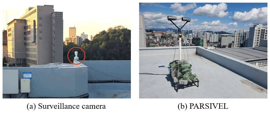
This study used a building's rooftop as the study site. The building is the Chung-Ang University Bobst Hall, located in the central region of Seoul in South Korea. It is located at 37∘30′13′′ N latitude and 126∘57′27′′ E longitude, at an elevation of 42 m. Figure 3 illustrates the CCTV (marked with a red circle) and PARSIVEL installed at the study site. The CCTV was used for the main analysis, and PARSIVEL was considered for verification purposes.
The CCTV model used in this study is DC-T333CHRX, developed by IDIS Ltd. The camera has a in. (7.6 mm by 5.7 mm) complementary metal oxide semiconductor (CMOS) with a height and width of 5.70 and 7.60 mm. The focal length is 4.5 mm, and the F number of the lens is 1.6. The shutter speed was set to s, and the frames per second (fps) was set to 30. The infrared ray distance is 50 m. The maximum permissible circle of confusion is 0.005 mm. The camera's resolution is 1080 pixels for the height and 1920 pixels for the width, but the cropped images (640 × 640 pixels) were considered for the analysis.
The PARSIVEL is a ground meteorological instrument that can observe the diameter and fall speed of precipitation particles (e.g., raindrops, snow particles, and hail). The meteorological information, including raindrop size, is used to estimate the quantitative precipitation amount and reveal the precipitation system's microphysical characteristics and development mechanism.
The PARSIVEL used in this study is the second version of the instrument manufactured by OTT in Germany, and it improved the observation accuracy of small particles. The PARSIVEL uses a laser-based optical sensor to send a laser from the transmitter and continuously receive it from the receiver (Fig. 4). As the laser beam moves from the transmitter to the receiver, the precipitation particle passes over the laser beam, and the size and velocity of the precipitation particle are observed (Nemeth and Hahn, 2005). The diameter and velocity of the particle are calculated by calculating the time that the particle passes through the laser and the laser intensity that decreases during the passage (Fig. 5).
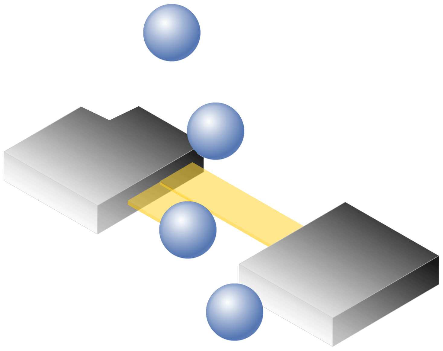
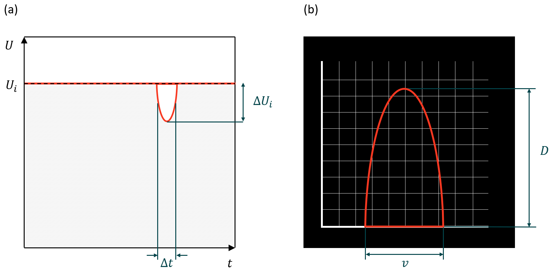
Figure 5(a) Signal changes whenever a particle falls through the beam anywhere within the measurement area. (b) The degree of dimming is a measure of the particle's size; together with the duration of the signal, the fall velocity can be derived.
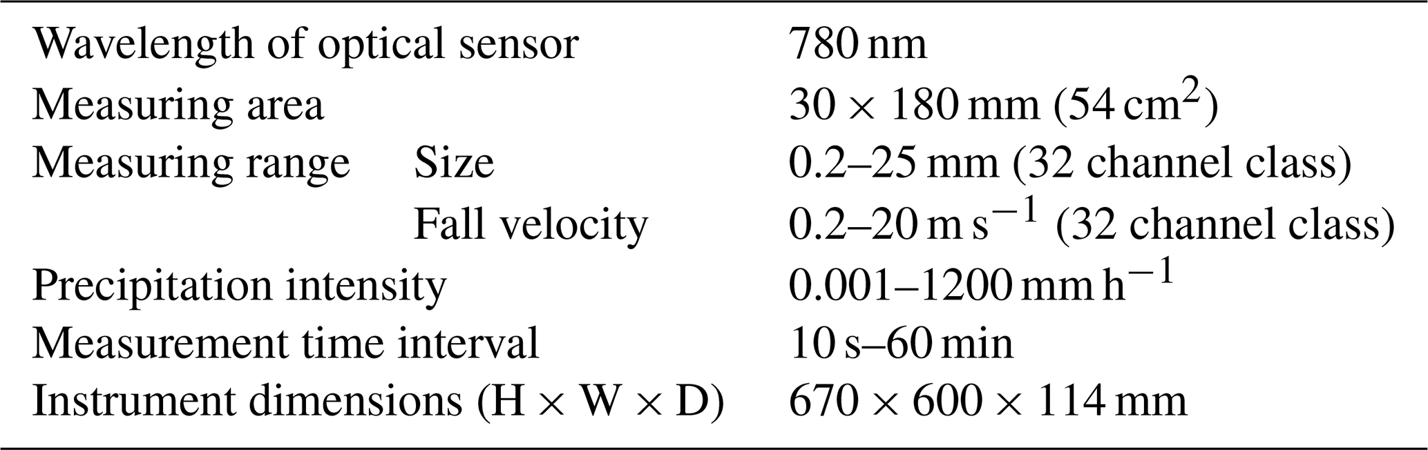
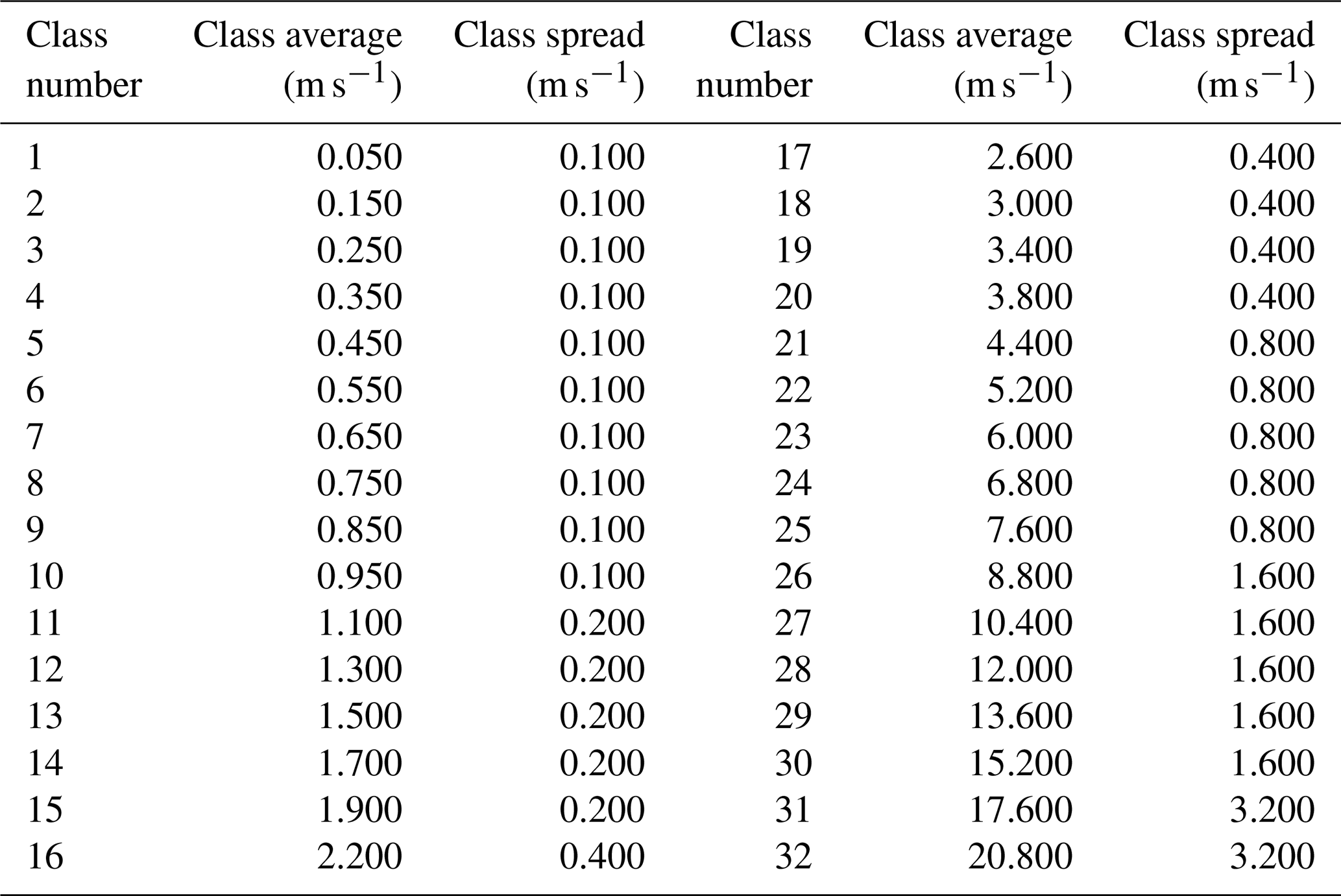
Parameters such as rain rate, reflectivity, and momentum of raindrops are calculated through particle concentration values for each diameter, and the falling speed channel is obtained through PARSIVEL observation. In this study, the temporal resolution of the observation data was set to 1 min. The particle diameters from 0.2 to 25 mm (Table A1 in Appendix) and fall velocity from 0.2 to 20 m s−1 (Table A2 in Appendix) can be observed by the PARSIVEL. The particle diameter and the fall speed each have 32 observation channels, so the number of observed particles for the time resolution set in 1024 channels (32 × 32) is observed. The first and second channels of the diameter are not included in the observable range of the PARSIVEL and are treated as noise. Therefore, the observation data of the first and second diameter channels were not considered in the actual analysis. The detailed information on the specifications of the PARSIVEL is presented in Table 2.
4.1 Rainfall event
We considered two rainfall events from 19:45 LST (local standard time) on 25 March 2022 to 06:15 LST on 26 March 2022 (case 1) and 21:00 LST on 5 September 2022 to 03:00 LST on 6 September 2022 (case 2). Figure 6 illustrates the hyetographs of the rainfall event considered in this study according to the time resolution. The total rainfall of case 1 and 2 is 19.5 and 48.7 mm, based on the PARSIVEL, respectively. The maximum rain rate is 10.0 and 20.7 mm h−1, based on the 1 min resolution, and 5.0 and 14.5 mm h−1, based on the 15 min resolution, for case 1 and case 2.
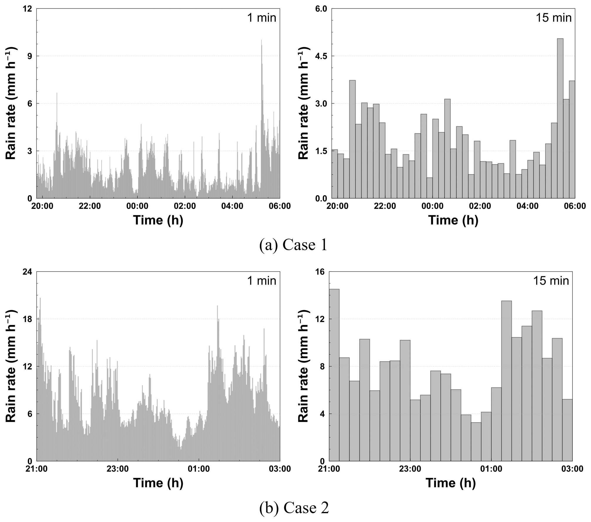
Figure 6Hyetograph of PARSIVEL and rain gauge observation data for the rainfall events considered in this study (left panels show the 1 min resolution; right panels show the 15 min resolution).

Figure 7Scatterplot of the rainfall amount every 1 h from the PARSIVEL observation and the rain gauge observation.
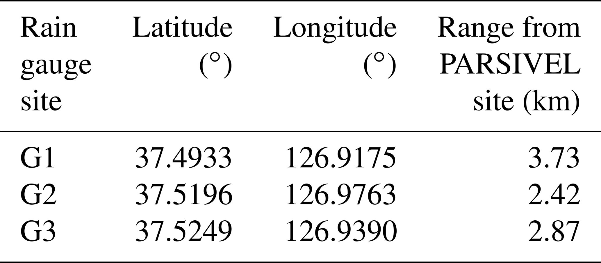
In order to secure the quantitative reliability of the PARSIVEL observation data, rain gauge observation data were used to verify the rainfall calculated through the PARSIVEL observation. The rainfall data used for verification are rain gauge observation data operated by KMA (Korea Meteorological Administration) installed less than 4 km from the PARSIVEL observation site (Table 3). The rainfall comparison period is from 14 September 2021 to 4 October 2022, including the period of the analysis case. Figure 7 shows scatterplots comparing hourly rain rates from rain gauges and PARSIVEL. As a result of comparison with the observation data at three rain gauge sites, it had low MAE (mean absolute error), RMSE (root mean square error), and MAPE (mean absolute percent error) values of less than 0.11 mm h−1, 0.6 mm h−1, and 8 %. Also, correlation values were more than 0.9.
4.2 Identifying rainfall streaks
The rain streaks were distinguished from the original raw images using the KNN-based algorithm described in Sect. 2.2. Accordingly, two parameters (history and dist2Threshold) were set to default values (500 and 400). The other parameter (detectShadows) was set to “false”. Figure 8 illustrates the raw, background, and rain streaks images, for an example time image (20:30:57 LST on 25 March 2022), scaled in yellow to make it easier to verify the visual change.
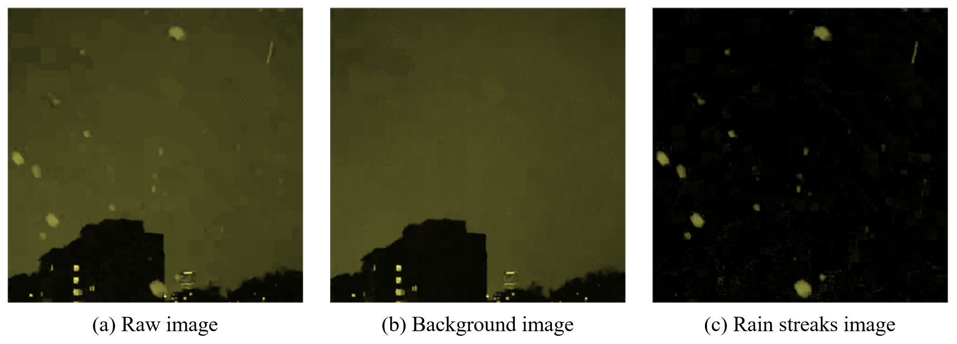
Figure 8Segmentation example of a raw image into background and rain streaks images based on a KNN-based algorithm (20:30:57 LST on 25 March 2022).
As confirmed in Fig. 8, adequate background separation performance can be achieved with the KNN-based method used in this study. Because it is an infrared camera, and the camera's exposure time is s, the length of rain streaks is relatively short. The longer the exposure time, the longer the raindrops appear on the image (Schmidt et al., 2012; Allamano et al., 2015). If the exposure time is too long, then some rain streaks may penetrate the image. In this case, it is difficult to estimate the rain streak length, which is a clue for estimating raindrop size.
The identification algorithm was implemented, using Anaconda Distribution on a workstation with an AMD Ryzen 5 5600X 6-Core Processor and 32 GB RAM. The computing time for the 15 min video was approximately 50 s, using only CPU computation. As described previously, the KNN-based algorithm used in this study has high-speed computing performance compared with various algorithms based on optimization, so it will likely have an advantage in real-time applications.
4.3 Estimation of DSD and rain rate
The rain streaks image presented in Fig. 8c was not considered for the final DSD estimation because of noise and factors other than rain caused by the sudden brightness change. As described in Sect. 3, a low-pass filter was first applied to the rain streaks image.
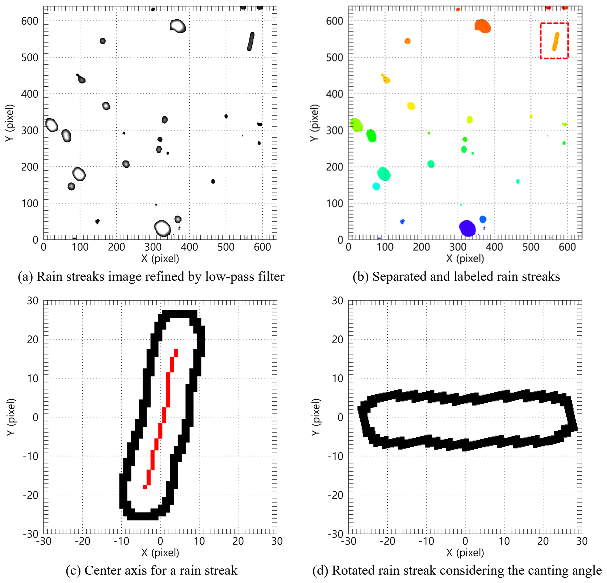
The 10 × 10 kernel was applied considering the total image size (640 × 640), and each grid value of the kernel was set to 0.01. The set kernel was filtered by convolution, pixel by pixel. Moreover, the convolution was performed once more using the following 2D kernel [0 1 0; −1 0 1; 0 −1 0] to highlight the rim of the rain streaks. A background layer with a value of 0 and a part not in the image were separated to extract the rain streaks, which were labeled one by one to identify each rain streak from the image. Figure 9a illustrates the example result after performing the processes described above in Fig. 8c. Each rain streak was then separated and labeled, as in Fig. 9b.
The border information of each rain streak needed to be obtained. The center axis was calculated by connecting the center (median) of the minimum pixel and maximum pixel values of the x axis for each y axis using border information. The angle of rain streak was obtained from the slope value obtained by calculating the linear function through the center axis's x and y pixel number values. Figure 9c is an example of the extraction of a rain streak extracted from the image of Fig. 9b.
The drop angle was then calculated, and the rain streak was rotated using the angle information. Raindrops can be broken up by strong wind or collisions between raindrops during falling. The maximum difference value between the minimum and maximum pixel number values of the y axis calculated using border information of the rotated rain streak was used to calculate the raindrop diameter and exclude the influence of the distorted shape of the rain streak by the break up (Fig. 9d; Testik, 2009; Testik and Pei, 2017). Figure 9d illustrates the result of the final process. If the rain streaks overlap, then the diameter of the raindrops can be estimated as large. To reduce the overestimation of raindrop diameter, this study tried to find the main central axis coordinates of overlapping rain streaks and set the longest central axis as the representative value. Then, we estimate the primary diameter by calculating the distance between each pixel value of the set central axis and the edge pixels of rain streaks.
Figure 10 illustrates the time series of the number concentration and Dm obtained from CCTV and PARSIVEL. From 19:45 to 23:50 LST, the maximum number concentration of lower than 1000 mm−1 m−3 was observed from the PARSIVEL observation, and from 20:00 to 20:10 LST, a number concentration lower than 100 mm−1 m−3 was observed. At 20:05 LST, large raindrops (of 3.8 mm) were observed, resulting in a sharp increase in Dm above 2 mm. In contrast, in the results based on CCTV images, the number concentration of less than 10 000 mm−1 m−3 was continuously demonstrated during the entire analysis period, and a number concentration greater than 5000 mm−1 m−3 was observed before 22:00 LST. Because the proportion of small drops was high, Dm was predominantly less than 1.5 mm.
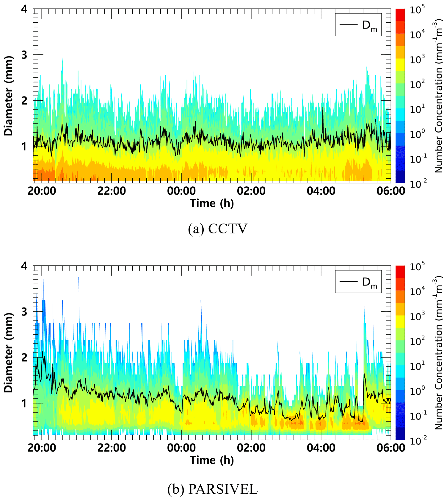
Figure 10Time series of number concentration and Dm (black line) from (a) the surveillance camera images and (b) the PARSIVEL observation data from 21:45 LST on 25 March to 06:00 LST on 26 March 2022 (case 1).
From 00:00 to 01:00 LST, both CCTV- and PARSIVEL-based data had a predominant maximum diameter of about 2.4 mm. At 00:35 LST, raindrops larger than 3.2 mm were observed in PARSIVEL, but raindrops less than 3 mm were not observed in CCTV. However, the number concentration of small diameters of 0.5 mm or less had similar values between 1000 and 5000 mm−1 m−3. Despite the difference in the maximum size of the drops, there was no predominant difference in the Dm because the number concentration of raindrops smaller than 1 mm had similar values.
From 03:00 to 05:30 LST, number concentrations higher than 5000 mm−1 m−3 in the raindrops smaller than 1 mm were observed using PARSIVEL. However, CCTV data revealed that number concentrations less than 5000 mm−1 m−3 were consistently observed. From 05:00 to 05:10 LST, the CCTV-image-based number concentration consistently appeared to be about 1.2 mm, whereas Dm was smaller than 0.7 mm in PARSIVEL. The cause for the rapid decrease in Dm of the PARSIVEL was that the CCTV-based maximum diameter is about 2.4 mm, which was similar to the PARSIVEL observation data, but the number concentration of 0.5 to 0.6 mm raindrops observed by PARSIVEL had a large value of more than 10 000 mm−1 m−3.
Figure 11 illustrates the average number concentration versus the diameter of raindrops calculated using the CCTV image and PARSIVEL observation data from 19:45 LST on 25 March to 06:00 LST on 26 March 2022. The PARSIVEL disdrometer data have a fixed raindrop diameter channel; thus, it can differ in number concentration, depending on the diameter channel setting. Therefore, in this study, the simulated DSD through the gamma model was also analyzed to compare the distribution of rainfall particles.
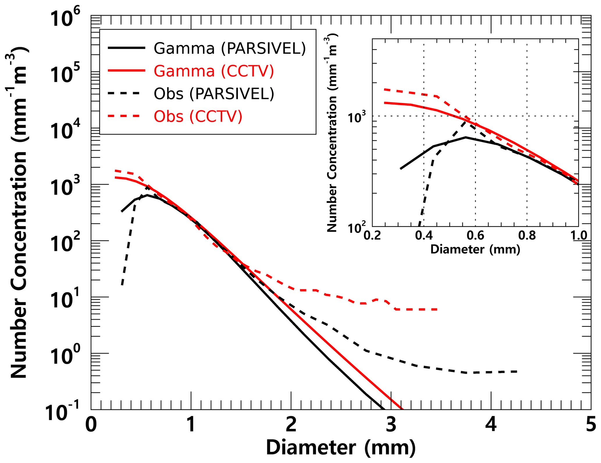
Figure 11Average number concentration versus diameter from the surveillance camera images and the PARSIVEL (case 1).
For raindrop diameters from 0.7 to 1.5 mm, the simulated and observed number concentrations produced similar values. However, above 1.5 mm, the model-based number concentration was under-simulated. From these results, in the precipitation case selected in this study, the gamma model appears limited for the simulation of the number concentration of raindrops larger than 3 mm. In diameters from 0.2 to 1.0 mm and above 1.5 mm, the number concentration obtained from CCTV images tended to be higher than that from the PARSIVEL observation. PARSIVEL observation data decreased sharply for diameters smaller than 0.3 mm. In contrast, CCTV gradually increased the number concentration as the diameter decreased.
Rainfall intensity was estimated based on the obtained number concentration from CCTV images and PARSIVEL. The near- (sn) and far-focus (sf) planes were calculated as 718 and 1648 mm from Eqs. (8) and (9). The DoF was calculated as 930 mm. The focal distance was set to 1 m, referring to previous studies (Dong et al., 2017; Jiang et al., 2019). The control volume was 2.9 m−3, applying Eq. (10) with the variables determined above. Figure 12 illustrates the rain rate time series calculated using CCTV images and PARSIVEL observation data. The increase or decrease in rain rate according to time change based on CCTV data followed the trend of rainfall intensity change based on PARSIVEL observation data.
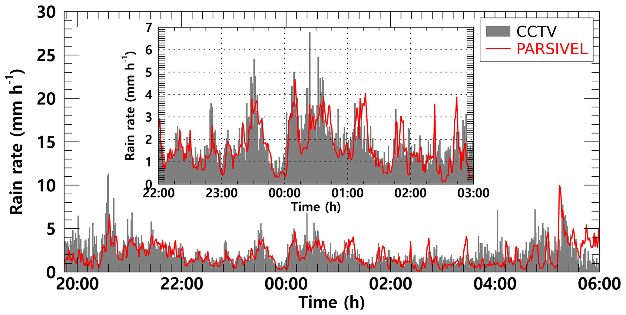
Figure 12The rain rate time series calculated from the surveillance camera images (gray bar) and PARSIVEL observation data (red line) from 21:45 LST on 25 March to 06:00 LST on 26 March 2022 (case 1).
At 20:37 LST, the PARSIVEL-based rain rate was 5.9 mm h−1, but the CCTV-based rain rate was overestimated to be higher than 10 mm h−1. On the other hand, the CCTV-based rain rate was underestimated by about 2 mm h−1 more than the PARSIVEL-based rain rate at 05:14 LST. Quantitative changes in CCTV-based rain rate showed a similar tendency to increase and decrease the number concentration of raindrops smaller than 1 mm and the maximum diameter. From 01:00 to 02:00 LST, when the number concentrations of CCTV and PARSIVEL had similar values, the rain rate also showed similar results.
Figure 13 illustrates the scatterplot of the average rain rate every 15 min from the PARSIVEL observation and the CCTV images. Uncertainty exists in the resolution of the rain gauge in the 1 min step. Accordingly, the time step for analysis is set to 15 min. The slope of the regression line was 0.71 because the CCTV-based rain rate tended to be overestimated at a rain rate of weaker than 2 mm h−1.

Figure 13Scatterplot of the average rain rate every 15 min from the PARSIVEL observation and the surveillance camera images (case 1). The red line is the linear regression. The scatterplot displays the correlation coefficient (CC), MAE, RMSE, and MAPE for R > 0 mm h−1, R < 2 mm h−1, and R ≥ 2 mm h−1 (sequentially from left to right).
The cumulative average rainfall intensity every 15 min was weaker than 10 mm h−1, concentrated at a rain rate of less than 6 mm h−1, so the correlation coefficient (CC) was 0.64. Furthermore, the MAE, RMSE, and MAPE were 0.61 mm h−1, 0.99 mm h−1, and 48 %. Differences according to rain rate can also be determined. The accuracy is higher at a rain rate smaller than 2 mm h−1 as a boundary. The MAE, RMSE, and MAPE were 0.29 mm h−1, 0.72 mm h−1, and 38 % for a rain rate of 2 mm h−1 or less and 0.58 mm h−1, 1.17 mm h−1, and 55 % for a rain rate above 2 mm h−1.
Table 4Statistical values of the rain rate and DSD parameters for case 1.
The statistical values of the rain rate and DSD parameters for the rainfall cases analyzed in this study are summarized in Table 4. The rain rate and Dm calculated using CCTV images were 0.459 mm h−1 and 0.025 mm more than the values calculated using PARSIVEL observation data on average, respectively. A high rain rate and Dm were caused by overestimating the number concentration for raindrops larger than 1.5 mm confirmed in Fig. 10. The number concentration for the small diameter (less than 0.3 mm) was higher in the CCTV data than in the PARSIVEL data. Due to the high concentration value of the number concentration of raindrops below 0.5 mm and above 2 mm, the CCTV-based rain rate had a large value.
In the Dm calculated through the PARSIVEL observation data, the concentration change in small drops over time was large, and the variance (0.063 mm) of Dm was large due to the rapid change in number concentration. The variability in the maximum diameter was greater in the PARSIVEL observation data, but the variance in the rain rate was greater in the CCTV data. The large variability in the concentration of raindrops below 3 mm affected the change in the rain rate. Also, due to the high number concentration of small drops, the skewness of the CCTV-based (1.903) rain rate had a higher value than that of the PARSIVEL-based (1.589) rain rate. The low variability (0.063 mm) in the Dm calculated from CCTV data means that the change in the shape of the raindrop size distribution was small, supported by the low variance of Λ (3.016 mm−1).
Figure 14 illustrates the time series of the number concentration and Dm obtained from CCTV and PARSIVEL for case 2. In both CCTV and PARSIVEL observation data, the number concentration for a diameter between 0.5 and 1.5 mm had a value between 500 to 5000 mm−1 m−3, and there was no significant change in the number concentration with time.
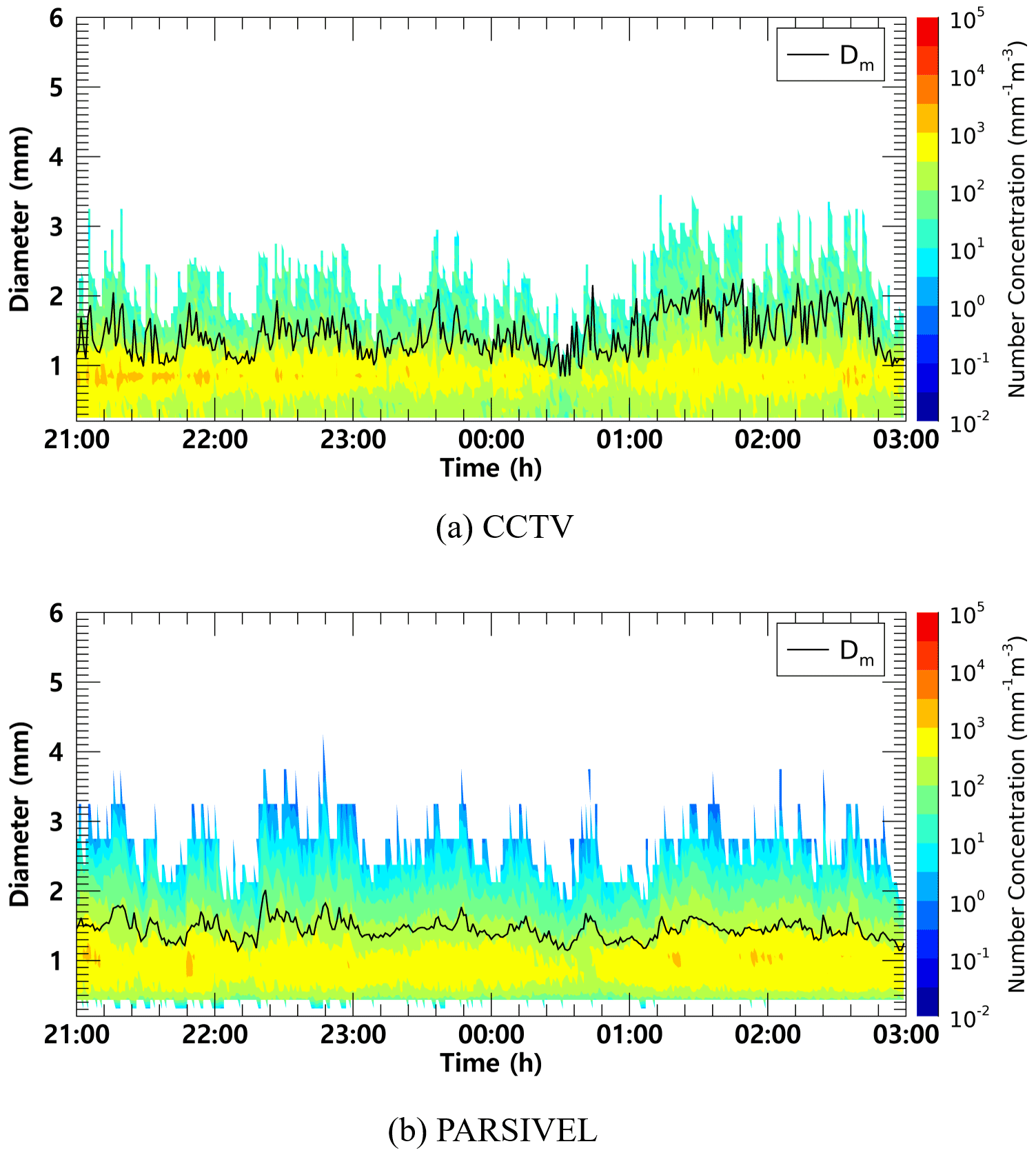
Figure 14Time series of number concentration and Dm (black line) from (a) the surveillance camera images and (b) the PARSIVEL observation data from 21:00 LST on 5 September to 03:00 LST on 6 September 2022 (case 2).
The maximum diameter also consistently had a value close to about 3 mm, and the Dm was also similar to about 1.5 mm because the maximum diameter and the number concentration of 1 mm intermediate drop had similar values.
From 01:00 to 02:30 LST, the maximum particle diameter through CCTV was overestimated, resulting in a large value close to 3.5 mm. As a result, the Dm value increased significantly to more than 2 mm. PARSIVEL data showed a sharp decrease in the number concentration of 1 mm drops at 00:30 LST, and an increase in Dm under the influence of the decreased number concentration. However, in the case of CCTV, only raindrops smaller than 1.5 mm were observed at the time, and there was a similar decrease in Dm (about 1.1 mm).
As clearly shown in Fig. 14, there was no significant difference in the number concentration according to the time change. The average number concentration distribution also showed similar results because the number concentration values were concentrated at 1000 mm−1 m−3 concentration in both observation instruments (Fig. 15). As in case 1, PARSIVEL observation data showed a tendency to underestimate in sections less than 0.5 mm and larger than 2 mm compared to CCTV data. The diameter section in which CCTV data are underestimated compared to PARSIVEL data was from 1 mm to 2 mm. Since the number concentration of the CCTV data was underestimated in this section, the rain rate based on the number concentration data was also underestimated compared to the rainfall intensity based on the PARSIVEL data.
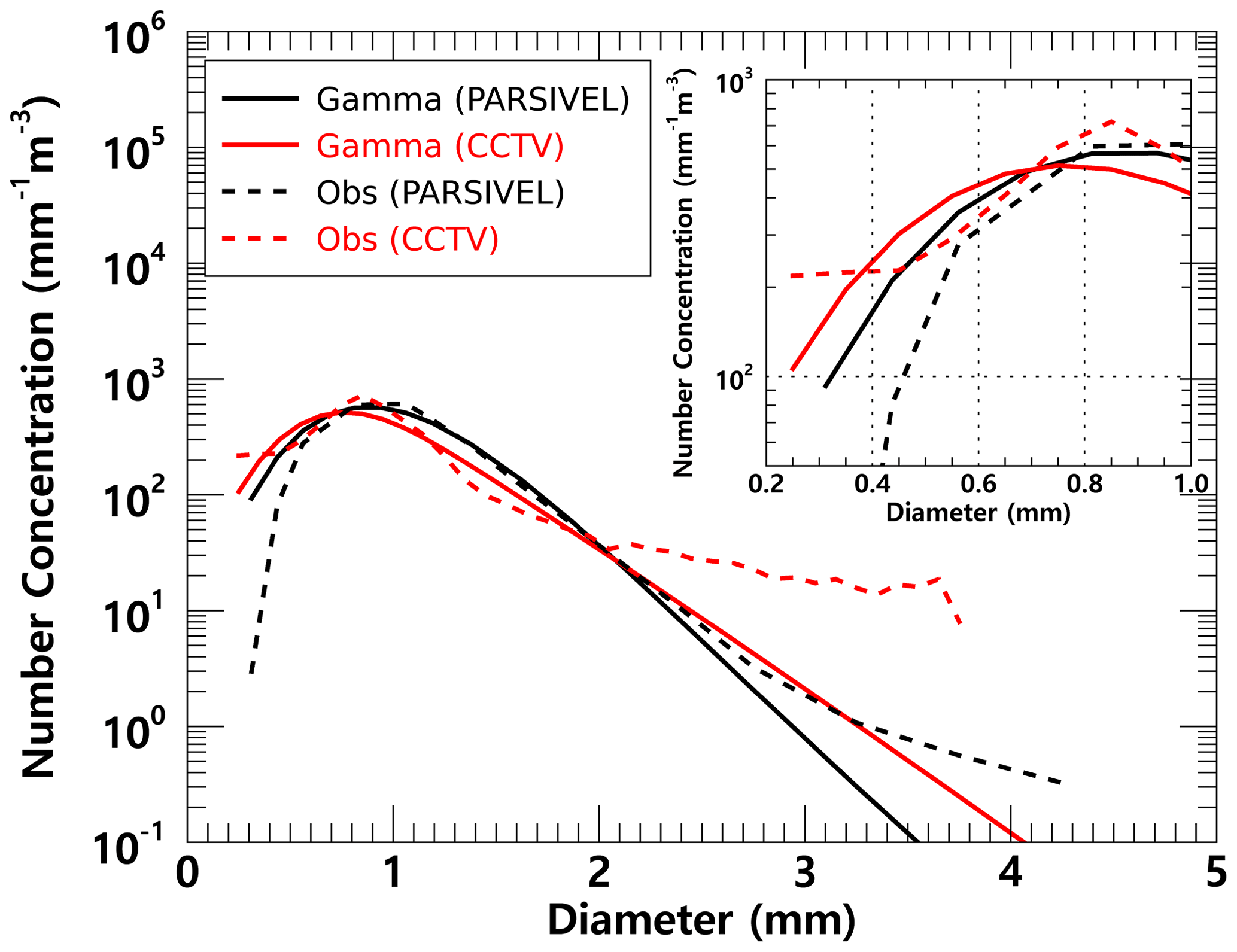
Figure 15Average number concentration versus diameter from the surveillance camera images and the PARSIVEL (case 2).
Between 21:00 LST on 5 September and 01:00 LST on 6 September, when the number concentration of about 1 mm raindrops is similar and the maximum diameter size is similar, the rain rate time series distribution has a value of about 5 mm h−1 and has a very similar flow. However, between 01:30 and 03:00 LST, which is a period with an overestimation of raindrop diameter in CCTV observation data, the increase and decrease in rain rate were similar. However, the magnitude of the increase and decrease in rain rate differed every 15 min. During that time, the maximum rain rate was less than 20 mm h−1 in the PARSIVEL observation data, while strong rainfall of 30 mm h−1 or more was observed in the CCTV observation data (Fig. 16).
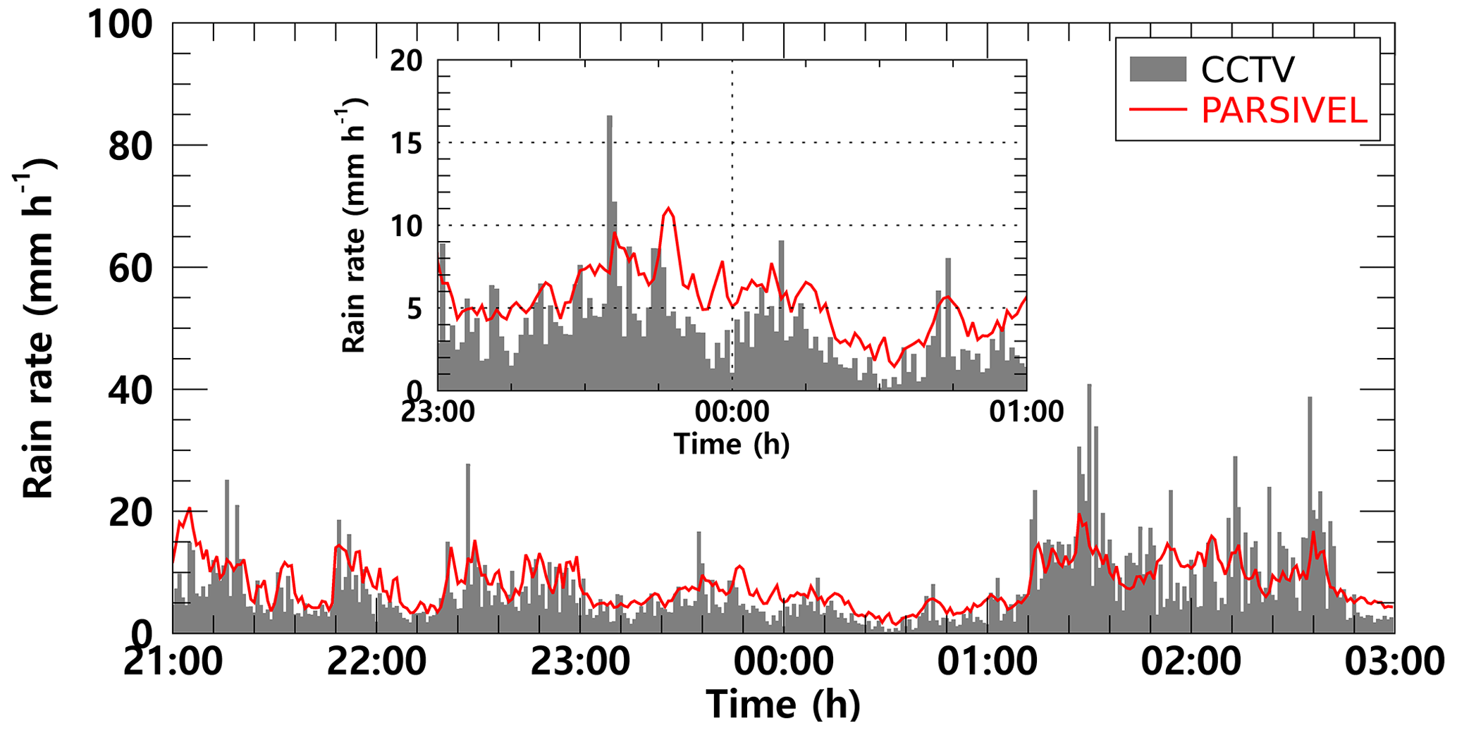
Figure 16The rain rate time series calculated from the surveillance camera images (gray bar) and PARSIVEL observation data (red line) from 21:00 LST on 5 September to 03:00 LST on 6 September 2022 (case 2).
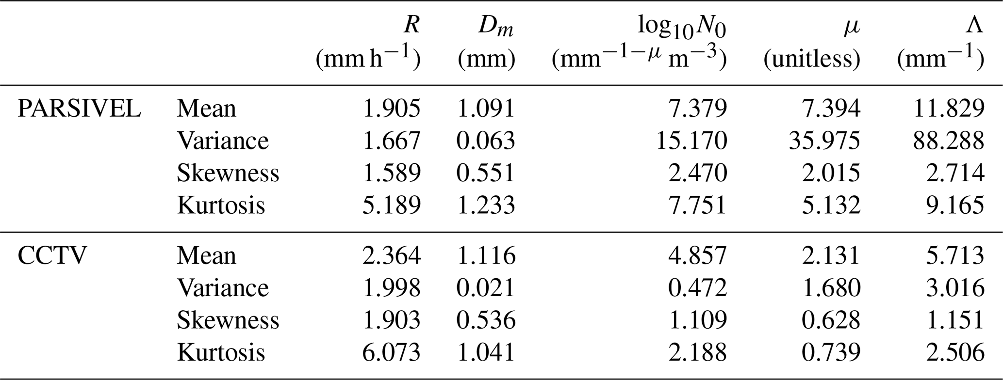
Table 5Statistical values of the rain rate and DSD parameters for case 2.
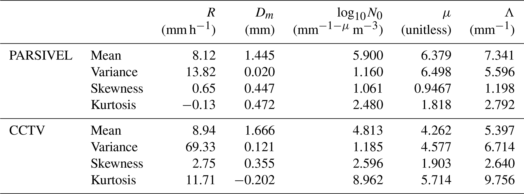
Figure 17 illustrates the scatterplot of the average rain rate every 15 min from the PARSIVEL observation and the CCTV images for case 2. Compared to case 1, case 2 was a strong rainfall case with a rain rate of about 8.94 mm h−1. Compared to the PARSIVEL observation data, the CCTV observation data showed a larger Dm by 0.221 mm, while the log 10N0 showed a small feature of 1.1 mm m−3. As the weight of medium and large drops over 1 mm increased, μ and Λ showed lower values of 4.262 and 5.397 mm−1, respectively (Table 5). According to the 15 min cumulative rain rate comparison result, the rain rate based on CCTV image data tends to be underestimated when it is less than 10 mm h−1. Conversely, there was a tendency to overestimate the rainfall period of 10 mm h−1 or more. This tendency was confirmed in case 1, which may be caused by recognizing overlapping rain streaks as a single big raindrop. MAPE had a low value of 0.3 % or less, regardless of the rain rate, and even though the rainfall intensity was relatively large compared to case 1, MAE and RMSE did not significantly increase. This is because there was no abnormally large value of CCTV rainfall during the rainfall period of case 2 compared to case 1.
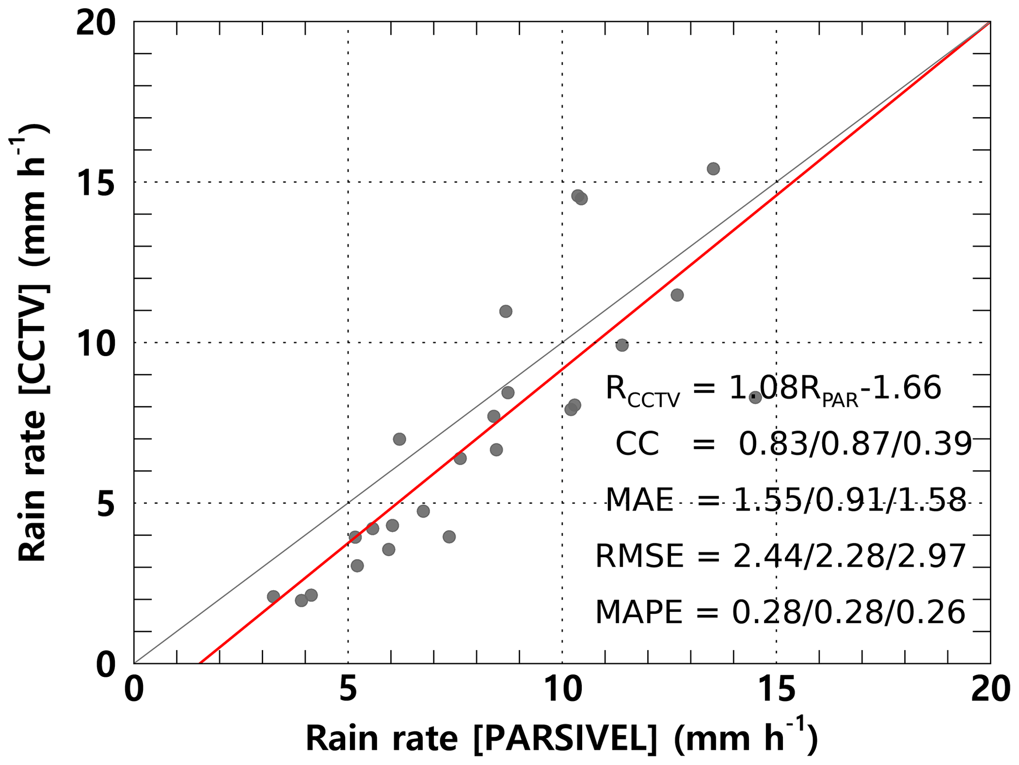
Figure 17Scatterplot of the average rain rate every 15 min from the PARSIVEL observation and the surveillance camera images (case 2). The red line is the linear regression. The scatterplot displays the CC, MAE, RMSE, and MAPE for R > 0 mm h−1, R < 5 mm h−1, and R ≥ 5 mm h−1 (sequentially from left to right).
This study estimated DSD with an infrared surveillance camera, based on which rainfall intensity was also estimated. Rain streaks were extracted using a KNN-based algorithm. The rainfall intensity was estimated based on DSD using physical optics analysis. A rainfall event was selected, and the applicability of the method in this study was examined. The estimated DSD was verified using a PARSIVEL. The results from this study can be summarized as follows.
The KNN-based algorithm illustrates suitable performance in separating the rain streaks and background layers. Furthermore, the possibility of separation for each rain streak and estimation of DSD was sufficient.
The number concentration of raindrops obtained through the CCTV images was similar to the actual PARSIVEL observed number concentration in the 0.5 to 1.5 mm section. In the small raindrops in the section of 0.4 mm or less, the PARSIVEL observation data underestimate the actual DSD. However, the CCTV image-based rain rate had an advantage over the raindrop-based data – the number concentration decreased rapidly as the number concentration gradually increased in the 0.2–0.3 mm diameter section.
The maximum raindrop diameter and number concentration of less than 1 mm produced similar results during the period with a high ratio of diameters less than 3 mm. However, the number concentration was overestimated during the period when raindrops larger than 3 mm were observed. The CCTV image-based data revealed that the rain rate was overestimated because of the overestimation of raindrops larger than 3 mm. After comparing with the 15 min cumulative PARSIVEL rain rate, the CCs – the MAE, RMSE, and MAPE of case 1 (case 2) – were 0.61 mm h−1 (1.55 mm h−1), 0.99 mm h−1 (1.43 mm h−1), and 48 % (44 %). The differences according to rain rate can be identified. The accuracy is higher at a rain rate smaller than 10 mm h−1 as a boundary.
The rain rate and Dm calculated using CCTV images exhibited similar average values. The overestimated number concentration of 1.5 mm or larger caused high kurtosis for the rain rate and Dm of CCTV-based data and a low μ value. Because of the high number concentration for raindrops larger than 3 mm of CCTV, the PARSIVEL observation data had a higher Λ value than the result based on the CCTV data.
In this study, DSD was estimated using an infrared surveillance camera; the rain rate was also estimated. Consequently, we could confirm the possibility of estimating an image-based DSD and rain rate obtained based on low-cost equipment in dark conditions. Though the infrared surveillance camera considered in this study will not be able to replace traditional observation devices, if future studies can be continued to secure robustness, then it will be an excellent complement to the existing observation system in terms of spatiotemporal resolution and accuracy improvement.
Table A1The representative diameter and spread for each diameter channel class.

Table A2The representative fall velocity and spread for each diameter channel class.
The raw videos and data used in the analysis can be downloaded from https://doi.org/10.6084/m9.figshare.c.6392430.v1 (Lee, 2023), and the sample codes are available at Zenodo https://doi.org/10.5281/zenodo.7601947 (jinwook213, 2023).
CJ, conceptualized the project. JBy did the data curation and formal analysis. JL and HJK did the analysis and interpretation. JBa led the investigation. JL prepared the original draft, and HJK reviewed and edited the paper. All authors have read and agreed to the published version of the paper.
The contact author has declared that none of the authors has any competing interests.
Publisher’s note: Copernicus Publications remains neutral with regard to jurisdictional claims in published maps and institutional affiliations.
This research has been supported by the Korea Meteorological Administration Research and Development Program (KMI2022-01910), by Basic Science Research Program through the National Research Foundation of Korea (NRF) funded by the Ministry of Education (2022R1I1A1A01065554 and 2022R1A6A3A01087041), and by the Chung-Ang University Graduate Research Scholarship in 2021.
This research has been supported by the Korea Meteorological Administration Research and Development Program (grant no. KMI2022-01910) and the National Research Foundation of Korea (grant nos. 2022R1I1A1A01065554 and 2022R1A6A3A01087041).
This paper was edited by Maximilian Maahn and reviewed by two anonymous referees.
Allamano, P., Croci, A., and Laio, F.: Toward the camera rain gauge, Water Resour. Res., 51, 1744–1757, https://doi.org/10.1002/2014wr016298, 2015.
Atlas, D., Srivastava, R. C., and Sekhon, R. S.: Doppler radar characteristics of precipitation at vertical incidence, Rev. Geophys., 11, 1–35, https://doi.org/10.1029/rg011i001p00001, 1973.
Avanzato, R. and Beritelli, F.: A cnn-based differential image processing approach for rainfall classification, Adv. Sci. Technol. Eng. Syst. J., 5, 438–444, https://doi.org/10.25046/aj050452, 2020.
Bouwmans, T., El Baf, F., and Vachon, B.: Statistical background modeling for foreground detection: A survey, in: Handbook of pattern recognition and computer vision, edited by: Chen, C. H., 4th edn., World Scientific, Singapore, 181–199, https://doi.org/10.1142/9789814273398_0008, 2010.
Cai, F., Lu, W., Shi, W., and He, S.: A mobile device-based imaging spectrometer for environmental monitoring by attaching a lightweight small module to a commercial digital camera, Sci. Rep., 7, 1–9, https://doi.org/10.1038/s41598-017-15848-x, 2017.
Colli, M., Lanza, L. G., La Barbera, P., and Chan, P. W.: Measurement accuracy of weighing and tipping-bucket rainfall intensity gauges under dynamic laboratory testing, Atmos. Res., 144, 186–194, https://doi.org/10.1016/j.atmosres.2013.08.007, 2014.
Deng, L. J., Huang, T. Z., Zhao, X. L., and Jiang, T. X.: A directional global sparse model for single image rain removal, Appl. Math. Model., 59, 662–679, https://doi.org/10.1016/j.apm.2018.03.001, 2018.
Dong, R., Liao, J., Li, B., Zhou, H., and Crookes, D.: Measurements of rainfall rates from videos, in: 2017 10th International Congress on Image and Signal Processing, BioMedical Engineering and Informatics, Shanghai, China, 14–16 October 2017, IEEE, 1–9, https://doi.org/10.1109/CISP-BMEI.2017.8302066, 2017.
Duthon, P., Bernardin, F., Chausse, F., and Colomb, M.: Benchmark for the robustness of image features in rainy conditions, Mach. Vis. Appl., 29, 915–927, https://doi.org/10.1007/s00138-018-0945-8, 2018.
Famiglietti, J. S., Cazenave, A., Eicker, A., Reager, J. T., Rodell, M., and Velicogna, I.: Satellites provide the big picture, Science, 349, 684–685, https://doi.org/10.1126/science.aac9238, 2015.
Friedrich, K., Kalina, E. A., Masters, F. J., and Lopez, C. R.: Drop-size distributions in thunderstorms measured by optical disdrometers during VORTEX2, Mon. Weather Rev., 141, 1182–1203, https://doi.org/10.1175/mwr-d-12-00116.1, 2013.
Garg, K. and Nayar, S. K.: Vision and rain, Int. J. Comput. Vis., 75, 3–27, https://doi.org/10.1007/s11263-006-0028-6, 2007.
Guo, B., Han, Q., Chen, H., Shangguan, L., Zhou, Z., and Yu, Z.: The emergence of visual crowdsensing: Challenges and opportunities, IEEE Commun. Surv. Tutor., 19, 2526–2543, https://doi.org/10.1109/comst.2017.2726686, 2017.
Guo, H., Huang, H., Sun, Y. E., Zhang, Y., Chen, S., and Huang, L.: Chaac: Real-time and fine-grained rain detection and measurement using smartphones, IEEE Internet Things, 6, 997–1009, https://doi.org/10.1109/jiot.2018.2866690, 2019.
Haberlandt, U. and Sester, M.: Areal rainfall estimation using moving cars as rain gauges – a modelling study, Hydrol. Earth Syst. Sci., 14, 1139–1151, https://doi.org/10.5194/hess-14-1139-2010, 2010.
Hua, X. S.: The city brain: Towards real-time search for the real-world, in: The 41st International ACM SIGIR Conference on Research & Development in Information Retrieval, New York, NY, USA, 8–12 July 2018, 1343–1344, https://doi.org/10.1145/3209978.3210214, 2018.
Jiang, S., Babovic, V., Zheng, Y., and Xiong, J.: Advancing opportunistic sensing in hydrology: A novel approach to measuring rainfall with ordinary surveillance cameras, Water Resour. Res., 55, 3004–3027, https://doi.org/10.1029/2018wr024480, 2019.
Jiang, T. X., Huang, T. Z., Zhao, X. L., Deng, L. J., and Wang, Y.: Fastderain: A novel video rain streak removal method using directional gradient priors, IEEE Trans. Image Process., 28, 2089–2102, https://doi.org/10.1109/tip.2018.2880512, 2018.
jinwook213: jinwook213/Rain_CCTV: J. Lee et al.: DSD and rain rate estimation with IR surveillance camera in dark conditions (v0.0), Zenodo [code], https://doi.org/10.5281/zenodo.7601947, 2023.
Kathiravelu, G., Lucke, T., and Nichols, P.: Rain drop measurement techniques: A review, Water, 8, 29, https://doi.org/10.3390/w8010029, 2016.
Keating, M. P.: Geometric, physical, and visual optics, 2nd edn., Butterworth-Heinemann, Oxford, UK, ISBN 0-409-90106-7, 2002.
Kidd, C., Becker, A., Huffman, G. J., Muller, C. L., Joe, P., Skofronick-Jackson, G., and Kirschbaum, D. B.: So, how much of the Earth's surface is covered by rain gauges?, B. Am. Meteorol. Soc., 98, 69–78, https://doi.org/10.1175/bams-d-14-00283.1, 2017.
Kim, J. H., Sim, J. Y., and Kim, C. S.: Video deraining and desnowing using temporal correlation and low-rank matrix completion, IEEE Trans. Image Process., 24, 2658–2670, https://doi.org/10.1109/tip.2015.2428933, 2015.
Lee, J.: Estimation of raindrop size distribution and rain rate with infrared surveillance camera in dark conditions, figshare [data set], https://doi.org/10.6084/m9.figshare.c.6392430.v1, 2023.
Li, Y., Tan, R. T., Guo, X., Lu, J., and Brown, M. S.: Rain streak removal using layer priors, in: 2016 IEEE Conference on Computer Vision and Pattern Recognition, Las Vegas, NV, USA, 27–30 June 2016, IEEE, 2736–2744, https://doi.org/10.1109/cvpr.2016.299, 2016.
Löffler-Mang, M. and Joss, J.: An optical disdrometer for measuring size and velocity of hydrometeors, J. Atmos. Ocean. Tech., 17, 130–139, https://doi.org/10.1175/1520-0426(2000)017<0130:aodfms>2.0.co;2, 2000.
Marshall, J. S. and Palmer, W. M.: The distribution of raindrops with size, J. Meteor., 5, 165–166, https://doi.org/10.1175/1520-0469(1948)005<0165:tdorws>2.0.co;2, 1948.
McCabe, M. F., Rodell, M., Alsdorf, D. E., Miralles, D. G., Uijlenhoet, R., Wagner, W., Lucieer, A., Houborg, R., Verhoest, N. E. C., Franz, T. E., Shi, J., Gao, H., and Wood, E. F.: The future of Earth observation in hydrology, Hydrol. Earth Syst. Sci., 21, 3879–3914, https://doi.org/10.5194/hess-21-3879-2017, 2017.
Michaelides, S., Levizzani, V., Anagnostou, E., Bauer, P., Kasparis, T., and Lane, J. E.: Precipitation: Measurement, remote sensing, climatology and modeling, Atmos. Res., 94, 512–533, https://doi.org/10.1016/j.atmosres.2009.08.017, 2009.
Nemeth, K. and Hahn, J. M.: Enhanced precipitation identifier and new generation of present weather sensor by OTT Messtechnik, in: WMO/CIMO Technical Conference, WMO IOM Report No. 82, WMO/TD-No. 1265, Geneva, Switzerland, 2005.
Nottle, A., Harborne, D., Braines, D., Alzantot, M., Quintana-Amate, S., Tomsett, R., Kaplan, L., Srivastava, M. B., Chakraborty, S., and Preece, A.: Distributed opportunistic sensing and fusion for traffic congestion detection, in: 2017 IEEE SmartWorld, Ubiquitous Intelligence & Computing, Advanced & Trusted Computed, Scalable Computing & Communications, Cloud & Big Data Computing, Internet of People and Smart City Innovation, San Francisco, CA, USA, 4–8 August 2017, IEEE, 1–6, https://doi.org/10.1109/UIC-ATC.2017.8397425, 2017.
Overeem, A., Leijnse, H., and Uijlenhoet, R.: Two and a half years of country-wide rainfall maps using radio links from commercial cellular telecommunication networks, Water Resour. Res., 52, 8039–8065, https://doi.org/10.1002/2016wr019412, 2016.
Qasim, S., Khan, K. N., Yu, M., and Khan, M. S.: Performance evaluation of background subtraction techniques for video frames, in: 2021 International Conference on Artificial Intelligence, Islamabad, Pakistan, 5–7 April 2021, IEEE, 102–107, https://doi.org/10.1109/ICAI52203.2021.9445253, 2021.
Rabiei, E., Haberlandt, U., Sester, M., and Fitzner, D.: Rainfall estimation using moving cars as rain gauges – laboratory experiments, Hydrol. Earth Syst. Sci., 17, 4701–4712, https://doi.org/10.5194/hess-17-4701-2013, 2013.
Rabiei, E., Haberlandt, U., Sester, M., Fitzner, D., and Wallner, M.: Areal rainfall estimation using moving cars – computer experiments including hydrological modeling, Hydrol. Earth Syst. Sci., 20, 3907–3922, https://doi.org/10.5194/hess-20-3907-2016, 2016.
Santhaseelan, V. and Asari, V. K.: Utilizing local phase information to remove rain from video, Int. J. Comput. Vis., 112, 71–89, https://doi.org/10.1007/s11263-014-0759-8, 2015.
Schmidt, J. M., Flatau, P. J., Harasti, P. R., Yates, R. D., Littleton, R., Pritchard, M. S., Fischer, J. M., Fischer, E. J., Kohri, W. J., Vetter, J. R., Richman, S., Baranowski, D. B., Anderson, M. J., Fletcher, E., and Lando, D. W.: Radar observations of individual rain drops in the free atmosphere, P. Natl. Acad. Sci. USA, 109, 9293–9298, https://doi.org/10.1073/pnas.1117776109, 2012.
Smith, P. L.: Raindrop size distributions: Exponential or gamma – Does the difference matter?, J. Appl. Meteorol. Climatol., 42, 1031–1034, https://doi.org/10.1175/1520-0450(2003)042<1031:rsdeog>2.0.co;2, 2003.
Testik, F. Y.: Outcome regimes of binary raindrop collisions, Atmos. Res., 94, 389–399, https://doi.org/10.1016/j.atmosres.2009.06.017, 2009.
Testik, F. Y. and Pei, B.: Wind effects on the shape of raindrop size distribution, J. Hydrometeorol., 18, 1285–1303, https://doi.org/10.1175/jhm-d-16-0211.1, 2017.
Tokay, A. and Short, D. A.: Evidence from tropical raindrop spectra of the origin of rain from stratiform versus convective clouds, J. Appl. Meteorol. Clim., 35, 355–371, https://doi.org/10.1175/1520-0450(1996)035<0355:eftrso>2.0.co;2, 1996.
Tripathi, A. K. and Mukhopadhyay, S.: Removal of rain from videos: A review, Signal Image Video P., 8, 1421–1430, https://doi.org/10.1007/s11760-012-0373-6, 2014.
Trnovszký, T., Sýkora, P., and Hudec, R.: Comparison of background subtraction methods on near infra-red spectrum video sequences, Proced. Eng., 192, 887–892, https://doi.org/10.1016/j.proeng.2017.06.153, 2017.
Ulbrich, C. W.: Natural variations in the analytical form of the raindrop size distribution, J. Appl. Meteorol. Clim., 22, 1764–1775, https://doi.org/10.1175/1520-0450(1983)022<1764:nvitaf>2.0.co;2, 1983.
Vivekanandan, J., Zhang, G., and Brandes, E.: Polarimetric radar estimators based on a constrained gamma drop size distribution model, J. Appl. Meteorol., 43, 217–230, https://doi.org/10.1175/1520-0450(2004)043<0217:preboa>2.0.co;2, 2004.
Wang, X., Wang, M., Liu, X., Glade, T., Chen, M., Xie, Y., Yuan, H., and Chen, Y.: Rainfall observation using surveillance audio, Appl. Acoust., 186, 108478, https://doi.org/10.1016/j.apacoust.2021.108478, 2022.
Yang, P. and Ng, T. L.: Gauging through the crowd: A crowd-sourcing approach to urban rainfall measurement and storm water modeling implications, Water Resour. Res., 53, 9462–9478, https://doi.org/10.1002/2017wr020682, 2017.
Yuter, S. E. and Houze Jr., R. A.: Measurements of raindrop size distributions over the Pacific warm pool and implications for Z–R relations, J. Appl. Meteorol., 36, 847–867, https://doi.org/10.1175/1520-0450(1997)036<0847:morsdo>2.0.co;2, 1997.
Zen, R., Arsa, D. M. S., Zhang, R., Er, N. A. S., and Bressan, S.: Rainfall estimation from traffic cameras, in: Database and Expert Systems Applications, edited by: Hartmann, S., Küng, J., Chakravarthy, S., Anderst-Kotsis, G., Tjoa, A., and Khalil, I., Springer, Cham, Switzerland, 18–32, https://doi.org/10.1007/978-3-030-27615-7_2, 2019.
Zivkovic, Z. and van der Heijden, F.: Efficient adaptive density estimation per image pixel for the task of background subtraction, Pattern Recognit. Lett., 27, 773–780, https://doi.org/10.1016/j.patrec.2005.11.005, 2006.
- Abstract
- Introduction
- Methodology
- Study site and observation equipment
- Application result
- Conclusion
- Appendix A: The diameter and fall velocity information for each diameter channel class
- Code and data availability
- Author contributions
- Competing interests
- Disclaimer
- Acknowledgements
- Financial support
- Review statement
- References