the Creative Commons Attribution 4.0 License.
the Creative Commons Attribution 4.0 License.
 | 10 Feb 2023
A fiber-optic distributed temperature sensor for continuous in situ profiling up to 2 km beneath constant-altitude scientific balloons
J. Douglas Goetz
Lars E. Kalnajs
Terry Deshler
Sean M. Davis
Martina Bramberger
M. Joan Alexander
A novel fiber-optic distributed temperature sensing instrument, the Fiber-optic Laser Operated Atmospheric Temperature Sensor (FLOATS), was developed for continuous in situ profiling of the atmosphere up to 2 km below constant-altitude scientific balloons. The temperature-sensing system uses a suspended fiber-optic cable and temperature-dependent scattering of pulsed laser light in the Raman regime to retrieve continuous 3 m vertical-resolution profiles at a minimum sampling period of 20 s. FLOATS was designed for operation aboard drifting super-pressure balloons in the tropical tropopause layer at altitudes around 18 km as part of the Stratéole 2 campaign. A short test flight of the system was conducted from Laramie, Wyoming, in January 2021 to check the optical, electrical, and mechanical systems at altitude and to validate a four-reference temperature calibration procedure with a fiber-optic deployment length of 1170 m. During the 4 h flight aboard a vented balloon, FLOATS retrieved temperature profiles during ascent and while at a float altitude of about 19 km. The FLOATS retrievals provided differences of less than 1.0 ∘C compared to a commercial radiosonde aboard the flight payload during ascent. At float altitude, a comparison of optical length and GPS position at the bottom of the fiber-optic revealed little to no curvature in the fiber-optic cable, suggesting that the position of any distributed temperature measurement can be effectively modeled. Comparisons of the distributed temperature retrievals to the reference temperature sensors show strong agreement with root-mean-square-error values less than 0.4 ∘C. The instrument also demonstrated good agreement with nearby meteorological observations and COSMIC-2 satellite profiles. Observations of temperature and wind perturbations compared to the nearby radiosounding profiles provide evidence of inertial gravity wave activity during the test flight. Spectral analysis of the observed temperature perturbations shows that FLOATS is an effective and pioneering tool for the investigation of small-scale gravity waves in the upper troposphere and lower stratosphere.
- Article
(6708 KB) - Full-text XML
- BibTeX
- EndNote


Distributed temperature sensing (DTS) uses a fiber-optic cable to obtain continuous profiles of temperature along the length of the fiber at a high time resolution. The sensing method is distinct from single-point fiber-optic techniques like fiber Bragg gratings in that it uses temperature-dependent light scattering in the Rayleigh, Brillouin, or Raman regimes within the fiber-optic core in conjunction with optical time domain reflectometry to acquire uninterrupted temperature along the longitudinal axis (Lu et al., 2019). Raman spectra DTS has gained popularity within the Earth sciences because it is a low-cost and simple method for measuring temperature in harsh environments and for sensing temperature gradients over large spatial domains relative to pointwise sensors (Tyler et al., 2009). Applications of DTS in environmental sensing have largely been centered around hydrologic and geologic research (Drusová et al., 2021; Henninges and Masoudi, 2021; Lagos et al., 2020; Selker et al., 2006; Sinnett et al., 2020; Tyler et al., 2009), but there has been increased interest in using DTS for atmospheric measurements over the last decade. Past atmospheric measurements with DTS can generally be categorized into three fields, including surface-layer-to-air interactions (Peltola et al., 2021; Petrides et al., 2011; Thomas et al., 2012), boundary layer dynamics (Egerer et al., 2019; Higgins et al., 2018; Keller et al., 2011; Fritz et al., 2021), and wind measurements (Sayde et al., 2015; van Ramshorst et al., 2020). In aerial studies, including measurements aboard tethered balloons (Keller et al., 2011; Fritz et al., 2021) and aboard an unmanned aircraft (Higgins et al., 2018), Raman spectra DTS was found to be reliable compared to traditional temperature sensors.
Here we describe a novel balloon-borne DTS system for atmospheric temperature profiling up to 2 km within the upper troposphere and lower stratosphere (UTLS). The UTLS is a globally important region of the atmosphere defined by its thermal structure, with a positive lapse rate in the troposphere, which is terminated at a cold point, and a subsequent shift to a negative lapse rate in the stratosphere. Temperature structure within the UTLS plays a pivotal role in the transport and chemistry of trace gases and aerosol. In the tropics, for example, stratospheric water vapor concentrations are controlled by the thermal structure of the tropical tropopause layer (TTL; Chang and L'Ecuyer, 2020; Fueglistaler et al., 2009; Randel and Jensen, 2013). Routine temperature measurements in this region are made by satellite sensors and a sparse network of equatorial radiosondes. Current space-based temperature measurements made by Global Navigation Satellite System (GNSS) radio occultation (GNSS-RO; e.g., the Constellation Observing System for Meteorology, Ionosphere, and Climate-2 – COSMIC-2) or nadir sounding (e.g., Advanced Microwave Sounding Unit – AMSU) provide near-global coverage, making them ideal for broad climate studies (Khaykin et al., 2017). However, nadir-sounding measurements have limited vertical resolution and are limited in their diurnal sampling, whereas GNSS-RO systems have highly variable spatial coverage. Both systems have horizontal resolutions ranging from a few kilometers to hundreds of kilometers. Balloon-borne radio soundings of atmospheric temperature are performed on a regular basis at numerous locations as part of the daily observations for aviation and meteorology. Radiosonde temperature measurements provide high vertical resolutions (5–100 m) over a large altitude range (∼ 0–30 km), but they only retrieve one vertical profile per flight and have a low temporal resolution, as they are typically performed once or twice per day. Thus, neither technique is ideal for investigating small-scale thermal structure and its evolution over space and time, which may occur due to gravity waves. The instrument described here overcomes both these limitations by collecting near-continuous, 3 m vertical-resolution temperature measurements through the vertical extent of the UTLS.
To investigate the thermal structure of the UTLS, the novel Fiber-optic Laser Operated Atmospheric Temperature Sensor (FLOATS) instrument was developed. The conception of the instrument was motivated by Stratéole 2, an international mission, to investigate dynamics, transport, and chemistry within the TTL and tropical lower stratosphere using constant-density balloons with flight durations up to 4 months (Haase et al., 2018). To test the FLOATS instrument concept, technical details, and operation, it was initially deployed on a shorter-duration, mid-latitude vented balloon flight. Temperature calibration and analysis techniques developed with the mid-latitude flight provided the necessary proof of concept for the long-duration Stratéole 2 flights and demonstrate that DTS is an effective tool for vertical profiling of the UTLS. The results of that flight are described herein as background for the two long-duration balloon flights that were completed during the 2021 Stratéole 2 scientific campaign.
2.1 Instrument overview
FLOATS is a DTS system that deploys up to 2000 m of fiber-optic cable, unreeled from an internal spool, below a high-altitude balloon gondola to obtain temperature profiles at 3 m vertical resolution with a minimum sampling period of 20 s. The instrument is comprised of three major components including a DTS, mechanical reeling system, and an end-of-fiber unit (EFU) sub-gondola (Fig. 1a). These components were developed for deployment aboard high-altitude balloons during the Stratéole 2 mission and are therefore designed to withstand harsh environmental conditions, run semi-autonomously with limited supervision from the ground, and meet the low-power, low-mass, and regulatory requirements of high-altitude ballooning. FLOATS was built to meet the requirements for a multi-month flight aboard a Centre National d'Études Spatiales (CNES) super-pressure balloon at a pressure level near 70 hPa, approximately 18 km, in the TTL, at latitudes between 15∘ N and 20∘ S. This region of the atmosphere is one of the coldest regions below the mesosphere, with mean temperatures ∘C (Fueglistaler et al., 2009).

Figure 1Illustration of the components of the FLOATS instrument (a) and optical system (b). Fiber-optic connections are depicted in panel (b) with green icons. The thermistor electrical symbols depicted in panel (b) are used to represent the location of a reference temperature sensor.
2.2 Optical system
The optical system of FLOATS, illustrated in Fig. 1b, is comprised of a commercial DTS optical bench, modified for high-altitude operation; control electronics; reinforced multimode fiber-optic cable; coiled sections of fiber-optic cable at uniform temperature; and reference temperature sensors. The sections of fiber-optic cable at uniform temperature combined with reference temperature sensors are identified as Ref. Section X in Fig. 1 and RSX in the text, where X is the reference section number. All of the components, with the exception of the fiber-optic cable when deployed for measurements, are contained within a temperature-controlled balloon gondola (−30 to 30 ∘C). The commercial optical bench is a Sumitomo Electric Industries, Ltd. FTR3000 instrument. The FTR3000 pulses 785 nm Class 1 laser light through the fiber-optic cable and senses the Stokes and anti-Stokes scattering at 760 and 810 nm, respectively, as a function of time using optical time domain reflectometry. For temperature calibration, the instrument contains a 25 m length of coiled unbuffered fiber laid on a temperature-controlled aluminum plate and immersed in a semi-solid gel (RS1). The FTR3000 with the factory single-point calibration system and a ∼1 min sample integration time has a manufacturer-specified temperature accuracy of ±0.7 ∘C at 500 m distance along the fiber, ±1.0 ∘C at 1000 m, and ±2.0 ∘C at 2000 m. The manufacturer reports a spatial resolution of 3 m, defined as the distance between the 10th and 90th percentile of a temperature step change.
In FLOATS, the FTR3000 is connected to a second 30 m section of unbuffered multimode fiber-optic cable coiled upon a mm aluminum plate and overlaid with self-leveling silicone adhesive with imbedded temperature sensors, all held within an ABS plastic box (RS2 in Fig. 1b). The coil is then connected to a fiber-optic rotary joint (Princetel, Inc.; RFCX-850-50) coupled to the reel system spool, which is in turn connected to up to 2000 m of deployable multimode fiber-optic cable.
The fiber-optic cable used for ambient temperature sensing outside of the balloon gondola is a size µm multimode fiber-optic with a single off-white coating of a proprietary liquid crystal polymer (LCP) manufactured by Linden Photonics, Inc. for a total diameter of 600±40 µm (Fig. 1b). The 600 µm diameter LCP fiber-optic was chosen to provide a minimum breaking strain of 140 N to meet CNES safety standards and a maximum breaking strain of 230 N for the EFU sub-gondola to be classified as a “light balloon” by ICAO regulatory standards (i.e., Rules of the Air ICAO, Appendix 4, Annex 2). The LCP-coated fiber-optic was also chosen because it exhibits low breaking-strain degradation, with 90 d equivalent exposure to stratospheric-level ultraviolet (UV) light.
The end-of-fiber-optic cable is attached mechanically, but not optically, to the EFU sub-gondola. Optical unions between sections of the fiber are component specific and, referencing Fig. 1b, include the following: (A) E2000-APC for the connection of FTR3000 to short-patch cord; (B) FC-APC for the patch-cord-to-RS2 connection;(C) FC-PC for the assembly of the reference section to the rotary joint to the spooled cable. Reference temperature sensors (i.e., 10 kΩ NTC thermistors and 100 Ω platinum RTD sensors) are placed on the aluminum plates of RS1 and RS2 for the temperature calibration procedures, which is discussed in Sect. 2.5.
2.3 Reeling system
The mechanical reeling system is designed to deploy the spooled fiber-optic cable during flight and to retract the fiber-optic cable at the end of flight. The system consists of a laser-sintered carbon-fiber-reinforced nylon spool driven by a brushless DC servomotor, planetary gearhead, and electromagnetic brake combination; a stepper-motor-driven “level-wind” carriage assembly; nylon redirect pulleys; and an electrical control system. The reeling system is functionally and mechanically similar to the system used by the balloon-borne water vapor, cloud, and temperature reel-down instrument RACHuTS, fully described in Kalnajs et al. (2021), with some minor differences. The DC servomotor assembly, for example, is rated for lower loads compared to the RACHuTS instrument (i.e., maximum design load of 19 N vs. 35 N) to meet differing mass requirements. Additionally, a larger spool diameter (12 cm) and wider-bend-radius pulleys for redirection of the cable compared to RACHuTS were chosen to minimize optical losses attributed to bends in the fiber-optic cable (Zeidler et al., 1976). The reeling system is capable of performing multiple deployments and retractions of the entire length of fiber or variable lengths and at variable speeds, depending on flight requirements. Typical deployment–retraction speeds are between 0.4 and 0.5 m s−1, and the system has a maximum speed of approximately 0.65 m s−1. Therefore, for a flight in which 2000 m of fiber-optic is required, it will take about 1 h to reach full deployment. It should be noted that at least 50 m of fiber-optic remains spooled on the reeling system at any point to act as a friction anchor and to prevent the loss of the cable and end-of-fiber unit while in flight.
2.4 End-of-fiber unit
The end-of-fiber unit is a 700 g self-contained sub-gondola used to acquire GPS position, ambient temperature, and pressure at the end of the FLOATS fiber-optic cable. The exterior of the EFU is a box made of extruded polystyrene foam with the dimensions of 12.5 cm ×12.5 cm ×20 cm. The fiber-optic cable is secured to the internal hollow-tube frame of the EFU. The closest 10 m of fiber-optic to the EFU are reinforced with a hollow-core ultra-high molecular-weight polyethylene (UHMWPE) braid with a breaking strain in excess of 400 N for dynamic shock load protection during the launch of FLOATS, at which point only the reinforced section is exposed to the load from the EFU. The interior is insulated with Cabot Thermal Wrap silica aerogel blankets and temperature controlled to −5 ∘C with a 1.6 W flexible amide heater wrapped on the battery pack. The sub-gondola is powered by a 24 Wh lithium ion battery pack that is charged with four 2 W photovoltaic arrays. Ambient temperature and pressure measurements are made with a Thermodynamical SENsor (TSEN) designed for sampling in the UTLS (Hertzog et al., 2007). The TSEN used by FLOATS is the same configuration used by the RACHuTS instrument, and a broader description can be found in Kalnajs et al. (2021). Previous measurements have shown the TSEN design to be effective at reducing solar radiative-heating biases normally associated with high-altitude measurements. TSEN has an accuracy and precision of 0.25 ∘C during the day and 0.1 ∘C at night (Hertzog et al., 2004). The TSEN temperature probe hangs ∼1 m below the EFU with small-gauge polytetrafluoroethylene (PTFE)-coated wire to reduce the effect of radiant heating from the EFU surface during daylight hours. The GPS measurements are made with a u-blox MAX-M8C module and have a specified position accuracy of 2.5 m. All engineering data, TSEN, and GPS data are collected every 10 s and transmitted via a long-range (LoRa) radio module to the instrument gondola.
2.5 DTS temperature calibration
The conversion of the temperature-dependent Raman backscattering per unit distance of the fiber-optic cable to ambient temperature was adapted from the single-ended non-duplexed DTS calibration methodologies provided in Hausner et al. (2011) and Suárez et al. (2011). In both methodologies, the temperature of a fiber-optic cable can be estimated by the following (Suárez et al., 2011, Eq. 1):
where T(z) is the temperature in K at the distance along the fiber z in meters, γ is the shift in energy between the incident laser wavelength and Raman-scattering wavelength in K, C is a dimensionless calibration parameter, Δα is the differential attenuation between the backscattered-Stokes and anti-Stokes intensities, and R(z) is the measured ratio between the power of the Stokes backscattering to the anti-Stokes backscattering. To retrieve temperature, γ, C, and Δα must be known. Once Δα is known for a given profile, ln [C] can be estimated as follows (Suárez et al., 2011, Eq. 4):
and γ can be estimated by the following (Suárez et al., 2011, Eq. 5):
In both equations, z1 and z2 are points or sections of fiber-optic cable at an externally measured uniform, but different, temperature. For FLOATS, T(z1) and T(z2) are the temperatures of RS1 and RS2, and they are measured independently (Fig. 1b). These sections are held at different temperatures by actively heating RS1 to a set point of 30 ∘C and allowing RS2 to passively heat to the internal gondola temperature, typically in the range of −30 to 30 ∘C.
With the Hausner et al. (2011) methodology, the Δα parameter of a DTS system can be independently calculated for each DTS profile by finding from a section of the fiber-optic cable at uniform temperature. In laboratory thermal-chamber experiments, the FLOATS reference sections were found to produce widely different Δα compared to the sensing fiber-optic, possibly because of dissimilarity in fiber-optic cable or because of low-temperature-related effects like strain on the fiber-optic and micro-bending loss (Hanson, 1979). The reference sections are therefore not reliable benchmarks for attenuation of the deployable fiber-optic cable in the UTLS environment. Additionally, under an ideal DTS setup, there would be no connections between components, hence zero loss. For FLOATS this is not possible, and the fiber-optic unions along the optical path of the DTS generate insertion loss or step losses in Raman-backscattering signal. Hausner et al. (2011) shows that step losses can be corrected by applying a linear offset to ln [R(z)], but this method likely assumes that the fiber-optic union and ±0.5 unit distance of the spatial resolution from the center of the union are at a uniform temperature. This is also not the case with FLOATS because the fiber-optic unions are between reference components held at different temperatures or optically undefinable sections like the spooled section of fiber. Optical unions in this orientation are required for integration of the optical components (i.e., reference sections and rotary joint) into the optical system and for assembly into the instrument gondola. Therefore, methods were developed to account for the temperature effects on Δα and optical union step loss in the FLOATS system by a two-step optimization scheme. These methods are fully described in Appendix A but are summarized here. First, the step loss between the reference sections internal to the gondola for the experiment is found empirically as the difference in Raman backscattering between RS2 and RS1 when the temperature offset between the two sections is equal to 0 ∘C. Second, the step loss between the remaining optical unions and Δα for each profile is determined by minimizing the absolute mean bias between the calculated temperature and the independently observed temperature of each reference section as outlined in Hausner et al. (2011). By these methods the parameters required to calculate temperature using Eq. (1) (i.e., γ, C, and Δα) can be determined dynamically for each profile within a given experiment.
2.6 Wyoming test flight
A validation flight of FLOATS was conducted on 22 January 2021 from Laramie, Wyoming (41.3∘ N, 105.7∘ W; 2228 m above sea level), to test and characterize FLOATS for the Stratéole 2 mission. The flight, named WY933, was aboard a 283 m3 Raven Aerostar zero-pressure vented balloon with a target constant-altitude float level of 20 km. The flight launch time was 05:43 local time, or Mountain Standard Time (MST). The flight train consisted of the balloon, a time- and altitude-controlled balloon cutaway device, a secondary balloon cutaway device, a parachute, a strobe light, a time-controlled parachute cutaway device, a radar transponder, and an instrument gondola. The instrument gondola was built with T-slotting framing rails with extruded polystyrene walls for insulation and approximated a Stratéole 2 gondola. Outside of the gondola was a GPS tracking device and an iMet-1-RSB radiosonde (Fig. 1a). The radiosonde provided high accuracy pressure, temperature, relative humidity, winds, and GPS position at the gondola flight level at a sampling rate of 1 s. The radiosonde telemetry was received by a mobile ground station. FLOATS was equipped with a 1200 m spool of fiber-optic cable. The length of cable was chosen to allow for full deployment of the fiber-optic cable within the ascent portion of the flight to retrieve fully deployed FLOATS temperature profiles during ascent. The reel system was designed to deploy the fiber at approximately 0.5 m s−1, and the targeted balloon ascent rate was approximately 5 m s−1, which allows for a maximum of 1200 m of fiber to be safely deployed during the 45 min ascent from the start of reel-out at 5 km to a float altitude of 19 km.
3.1 WY933 flight summary
Figure 2 shows the instrument gondola GPS altitude and the vertical distance between the gondola and EFU determined by the EFU GPS as a function of time for WY933. The fiber-optic reel-out started at 05:58 MST, 15 min after launch, at a GPS altitude of 5820 m. The reel-out completed at approximately 06:30 MST with the complete deployment of 1167 m of fiber-optic cable, based on optical length, at an altitude of 13 600 m. The gondola reached its float altitude of 19 140 m at 06:45 MST, about 110 km downrange from the launch site. The fiber-optic remained fully deployed until 08:15 MST, when automated fiber-optic retraction began. The gondola was cut away after drifting horizontally for nearly 90 km. All flight control times were designed to provide adequate time for ascent, fiber-optic reeling, fully deployed temperature profiling, and parachute descent while maintaining a radio-communicable flight distance. During the flight, the internal temperature of the gondola ranged from −17 to 14 ∘C, with an average (± standard deviation) of ∘C at float altitude.
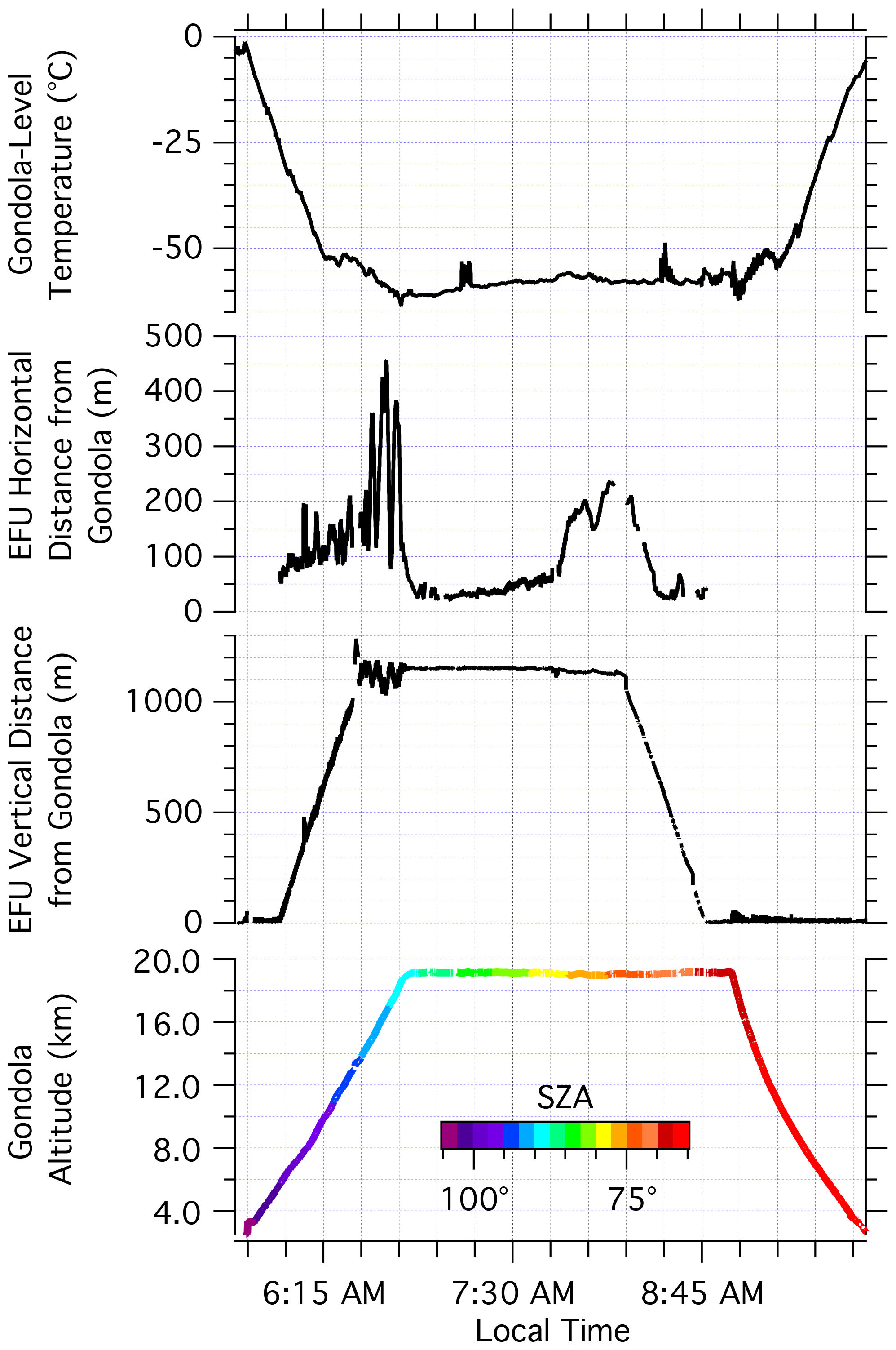
Figure 2Summary of flight conditions of the 22 January 2021 WY933 zero-pressure balloon fight. Altitude-adjusted solar zenith angle is displayed in rainbow.
FLOATS retrieved a total of 381 DTS profiles with a sampling period of 20 s and a deployment length greater than 8 m. The gondola crossed the tropopause at about 11 km with a temperature of −53 ∘C. At float altitude, the ambient temperature ranged from −62.6 to −54.8 ∘C, with an average of −57.9 ∘C (Fig. 2). The iMet-1-RSB temperature, however, did report large spikes in temperature – at 07:15 and 08:30 MST, for example – which is suggestive of the temperature sensor being in direct sunlight and poorly ventilated for short periods of the flight. Based on the gondola-altitude-adjusted solar zenith angle (SZA) shown in Fig. 2, SZA <90∘ was observed by the gondola at about 16 km or 06:40 MST. The observed SZA less than 90∘ reveals that FLOATS was in some degree of direct sunlight for the entirety of the time that the fiber-optic was fully deployed. Thus, the effect of solar radiative heating on the fiber-optic cable and the resulting DTS temperature cannot be assessed from WY933. Solar radiative heating is a known concern for ground-based atmospheric DTS systems (de Jong et al., 2015), but ventilation by vertical wind shear along the length of the fiber-optic cable will likely reduce the effect of solar heating on the FLOATS temperature profiles for distances greater than a few meters below the gondola. Vertical wind shear and radiative heating will be addressed in the Stratéole 2 campaign, where large daytime and nighttime datasets will be available.
Unfortunately, the EFU TSEN thermistor was damaged during the WY933 launch and was unable to report end-of-fiber temperature, although the position of the EFU was recorded. Because of the damaged sensor, modifications to the temperature calibration method discussed in Sect. 2.2 and Appendix A were made to retrieve temperature from the WY933 Raman-backscattering profiles. These modifications are unique for the ascent–descent profiles and the float altitude profiles. For the ascent–descent profiles, RS4 temperature was derived from the iMet-1-RSB temperature profile by matching GPS altitudes from radiosonde and the EFU. For the float altitude profiles, a static Δα was estimated from the ascent profiles closest to the float level. The float-level temperature profiles were then retrieved from a three-reference-section calibration where only the rotary joint step loss value was optimized, as discussed in Appendix A.
3.2 End-of-fiber position
The position of the end of the fiber is a useful tool to evaluate the position of any point along the fiber and thus the geospatial position of any FLOATS distributed temperature measurement. As seen in Fig. 2 the end-of-fiber altitude relative to the instrument gondola altitude during WY933 is not constant even after the fiber-optic is fully deployed. For example, the vertical distance between the gondola oscillated in the lower stratosphere before reaching float altitude. These oscillations are related to the horizontal offset between the instrument gondola and EFU estimated with the Haversine formula to calculate great-circle distance. The EFU horizontal distance from the instrument gondola is given in Fig. 2 and shows an inverse relationship to the vertical distance. Here, the maximum horizontal distance was observed during the oscillation period prior to when float altitude was reached and then dampened to a minimum of 27 m at the start of the float altitude period. The horizontal separation increased with time during the float altitude period and reached another maxima directly prior to the fiber-optic reel-in. The inverse relationship between the vertical and horizontal displacements of the end of fiber suggests that a right-triangle model within a Cartesian plane may be used to describe or partially describe the position of the entire fiber relative to the gondola.
Using the right-triangle model, by defining the hypotenuse as the shortest distance between the gondola and the EFU, the average distance between them while fully deployed was estimated to be 1153±7 m. Given the spatial inaccuracies of both GPS units and other uncertainties, the estimated orthogonal distance compares well with the 1167 m deploy distance estimated by DTS optical length. Therefore, there was likely little to no curvature in the deployed fiber-optic cable during WY933, and the right-triangle model can be used to evaluate the geospatial position of the FLOATS fiber-optic. Curvature of the deployed fiber-optic can lead to difficulties interpreting geospatial results and therefore should be flagged in any dataset. A case where the calculated hypotenuse is significantly shorter than the optical length of the fiber-optic cable would suggest that the fiber is exhibiting significant curvature, resulting in increased uncertainty in the derived geometric altitude for positions along the fiber.
Figure 3a gives the three-dimensional translation of the end-of-fiber position by showing the position of the end of fiber in degrees from the nadir view of the gondola as a function of geographic bearing for the ascent and float altitude phase of flight. Over the course of the WY933 flight, the end-of-fiber angle from nadir had an average value of 6.7∘ ± 5.0∘ with a range of 1.0 to 29∘. The angles were observed during all periods of ascent, and the fiber-optic exhibited both pendulum and rotational patterns, suggesting effects from wind shear along the ascent path (Fig. 3b), which will be explored further in Sect. 4.5. After ascent, the rotational motions are dampened, and the angle from nadir is reduced to less than 10∘ (Fig. 3a). For reference, a 10∘ offset from nadir produces a vertical displacement of about 1.5 % at the end of the fiber compared to a nadir profile. The same degree of offset generates a horizontal displacement of about 17 % compared to a nadir profile. The displacements may be corrected for by applying the right-triangle model to estimate the altitude of all points along the fiber. However, the application of the model depends on the FLOATS dataset and minimum error needed for interpretation of those results. The above geospatial methods provide a framework that can be used to evaluate the quality of future FLOATS temperature profiles.

Figure 3Polar graphs of (a) the end-of-fiber position angle in degrees with respect to nadir from the gondola and geographic bearing and (b) the wind speed in m s−1 and wind direction in degrees observed at the gondola level. Markers (rainbow) are colored by the local time (MST).
3.3 DTS performance
The onboard reference temperature sensors (Fig. 1b) were used to evaluate the performance of the DTS temperature profiles from the ascent and float altitude of WY933. Since the EFU TSEN was damaged, only the gondola-level iMet-1-RSB temperature coincident to the EFU altitude could be used for the RS4 temperature during the ascent phase. The float altitude profiles were then calibrated using only the internal reference sections and RS3. For each reference section, every 1 m point within that section was used to find the root-mean-square error compared to its respective sensor as follows:
where Ti is the DTS temperature of a given point within a reference section with n observations, and Tobs is the reference section temperature.
The average RMSEs for each reference section during ascent after the fiber-optic was fully deployed and at float altitude are shown in Table 1. Generally, the errors observed with the DTS observation in RS1 and RS2 were less than 0.3 ∘C from all periods of flight and are representative of the minimum error in the measurement. The low error associated with these sections is likely because the sections are used to calculate the calibration parameters C and Δα, as shown in Eqs. (2) and 3. Also, because the sections are close to the incident laser, there is large signal to noise in the Raman backscattering. This is a known characteristic of DTS. The FTR3000 data sheet, for example, shows a 1.4 ∘C difference in temperature accuracy between measurements at 500 m compared to 2000 m using the manufacturer's calibration. The ascent-phase reference sections outside of the gondola were found to have RMSE of 1.2±1.4 ∘C (RS3) and 1.2±0.6 ∘C (RS4), respectively. The comparable RMSE observed with RS3 and RS4 and the larger standard deviation observed with RS3 were unexpected and do not follow what is known about accuracy as a function of distance down the fiber. Similar RMSEs were observed between all ascent profiles and those when the fiber-optic was fully deployed. During float, the DTS performed better than during ascent with a decrease of almost 72 % in error observed with RS3 (Table 1). The RMSE during float for RS4, however, is unknown because of the damaged EFU TSEN. During the retraction period of the float altitude phase of flight, the DTS at RS3 performed poorly with an increase of 2 orders of magnitude in RMSE.
Table 1The average and standard deviation of the RMSE of the FLOATS DTS reference section temperature compared to the reference temperature sensors for the ascent and float-level profiles.
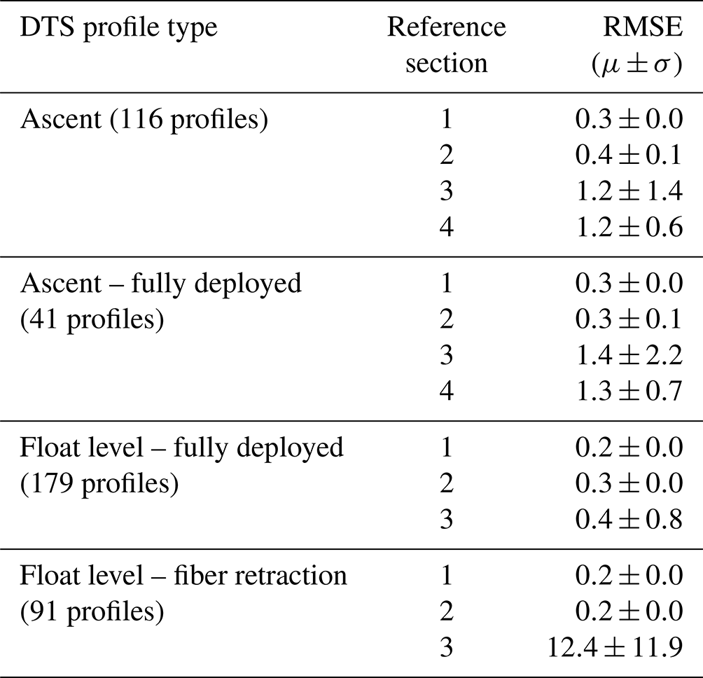
Based on the error statistics from the reference sections, there are several conclusions that can be applied to the interpretation of the temperature profiles as a whole. First, the Raman-backscattering profiles from the fiber-optic retraction period cannot be used for temperature retrievals. The reason for the large error observed during retraction is not fully understood, but it is thought to be due to damage to the optical core of the fiber-optic cable, temperature-induced micro-bend losses, or a combination of both. The same error was not observed during the deployment phase, suggesting that the temperature of the fiber-optic being spooled or unspooled may have an effect on optical losses. For reference, the WY933 reel was spooled in laboratory conditions and deployed at gondola temperatures greater than −10 ∘C, while the fiber was retracted at temperatures less than −55 ∘C. The effect of spooling or unspooling temperatures may also play a part in the increased RMSE observed with RS3 between the fully deployed ascent and fully deployed float altitude phases. The recently deployed fiber-optic may not have reached full temperature stabilization outside of the gondola within the 20 s sampling period and, hence, may have caused the observed differences between the reference temperature and DTS temperature. The similar or greater RMSE observed with RS4 during ascent compared to RS3 suggests that the response time of the DTS may be slower than the change in ambient temperature during ascent. This is a reasonable assumption because the average ascent rate of the balloon was 4.3 m s−1; therefore, there was likely some vertical “smearing” of the DTS temperature over 20 s.
To further evaluate the performance of the FLOATS temperature profiles, full ascent period profiles are compared to the iMet-1-RSB aboard the instrument gondola. Figure 4 shows the FLOATS temperature profiles averaged into 75 m altitude bins from 6.5 to 19 km. Seventy-five meters averaging was chosen to reflect the vertical resolution of FLOATS during the ascent portion of the flight based on an average ascent rate of 4.3 m s−1, fiber-optic deployment speed of 0.45 m s−1, and DTS sampling period of 20 s. At this averaging interval, “smearing” of the FLOATS temperature profiles due to vertical motion is reduced and suitable for comparison to the ∼4 m native vertical resolution of the iMet1-RSB temperature sensor. The number of profile points averaged into each bin presented in Fig. 4a is colored by an orange gradient on the trace showing that upwards of 1000 individual 1 m samples within each altitude bin were included in the ascent average. The standard deviation, shown in gray, indicates that there was some variability in the DTS temperature at a single altitude, with an average standard deviation of 2.1 ∘C and a range of 1.1 to 5.0 ∘C (Fig. 4). Figure 4 also shows increased standard deviation values with altitude, starting at about 14 km, and the position of increased variability is coincident with the altitude where full fiber-optic deployment was achieved during ascent (Fig. 2). The changing standard deviation possibly indicates that variability in the FLOATS ascent profile increased with sample number at the far end of the fiber-optic, where different atmospheric temperatures may have been sampled at each altitude due to changing geographic position or atmospheric dynamics. The FLOATS ascent average compares well with the radiosonde altitude binned average at the same altitude and follows the same vertical trends. The absolute difference between the two ascent profiles shows that the sensors measured a maximum of 2.8 ∘C of difference, with a majority of the measurements <2.0 ∘C (Fig. 4b). We use the mean absolute error (MAE), which is defined as
or the average of the absolute difference given in Fig. 4b, where Tobs is the average iMet temperature and Tavg is the average FLOATS temperature for a given 75 m altitude bin i, and n is the number of altitude bins. The MAE was found to be 0.85 ∘C for the DTS ascent profile compared to the reference temperature profile. The 0.85 ∘C difference of the FLOATS ascent profile and the similar vertical structure of the two sensors, under rapidly changing atmospheric conditions, provide encouraging results for the effectiveness of the DTS temperature calibration methodology provided in this work and give confidence for the float-level temperature retrievals where RS4 calibration values are not available.
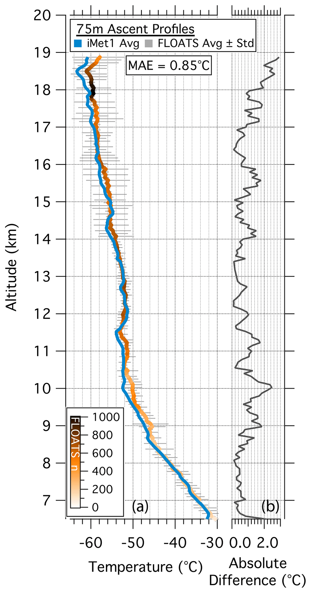
Figure 4(a) Ascent temperature profiles of the gondola-level iMet radiosonde (blue line) and the DTS scans averaged into 75 m bins. The DTS average temperature (orange gradient) is colored by the number (n) of 1 m DTS sample points averaged for each 75 m bin. The standard deviation of the 75 m DTS bins is shown in gray. (b) Ascent profiles of the absolute difference between the iMet radiosonde and DTS average temperature.
3.4 Float-level temperatures
The three-reference-section-calibrated temperatures at the WY933 float altitude can be seen in the curtain plot found in Fig. 5a. In the figure, FLOATS profile temperatures are displayed as a function of altitude and local time. At the start of float altitude, FLOATS records a relatively flat temperature profile near −61 ∘C, reaching from ∼18 to ∼19.1 km with a cold band centered at 18.5 km. This cold band was observed to have a minimum temperature of −63.0 ∘C and is consistent with the local cold-point temperature of −63.5 ∘C and the thermal structure observed in the iMet-1-RSB ascent profile at the same altitude (Fig. 5c). Looking at the first 2 min of FLOATS measurements at float altitude, the average profile was found to have an MAE of 1.0 ∘C compared to the iMet ascent profile. At about 06:55 to 07:05 MST the segment of profile at altitudes greater than 18.55 km began to warm to temperatures between −59 and −60 ∘C, and the lower altitudes in the profile remained at a consistent temperature, with an average of −60.8 ∘C (Fig. 5a). Warming at the top half of the FLOATS fiber-optic that was not observed at the bottom suggests that the instrument was entering a warm layer at those altitudes. It is unlikely that the observed warming trend was due to solar heating of the cable, even as the SZA reached 85∘ during that period (Fig. 5b). A similar warming trend and structure were observed by the onboard radiosonde during the descent of the gondola. Furthermore, the structure and evolution of the wind field, or wind shear, can be estimated by the wind speed profiles calculated from the horizontal displacement of the payload during ascent and descent (Appendix B). Based on the wind shear profiles, it is clear that large sections of the fiber-optic cable were well ventilated at altitudes greater than 200 m below the gondola and that the wind shear profiles within the float-level domain were not static. Additionally, there is no apparent correlation between low ventilation and elevated temperatures within the FLOATS temperature retrievals.
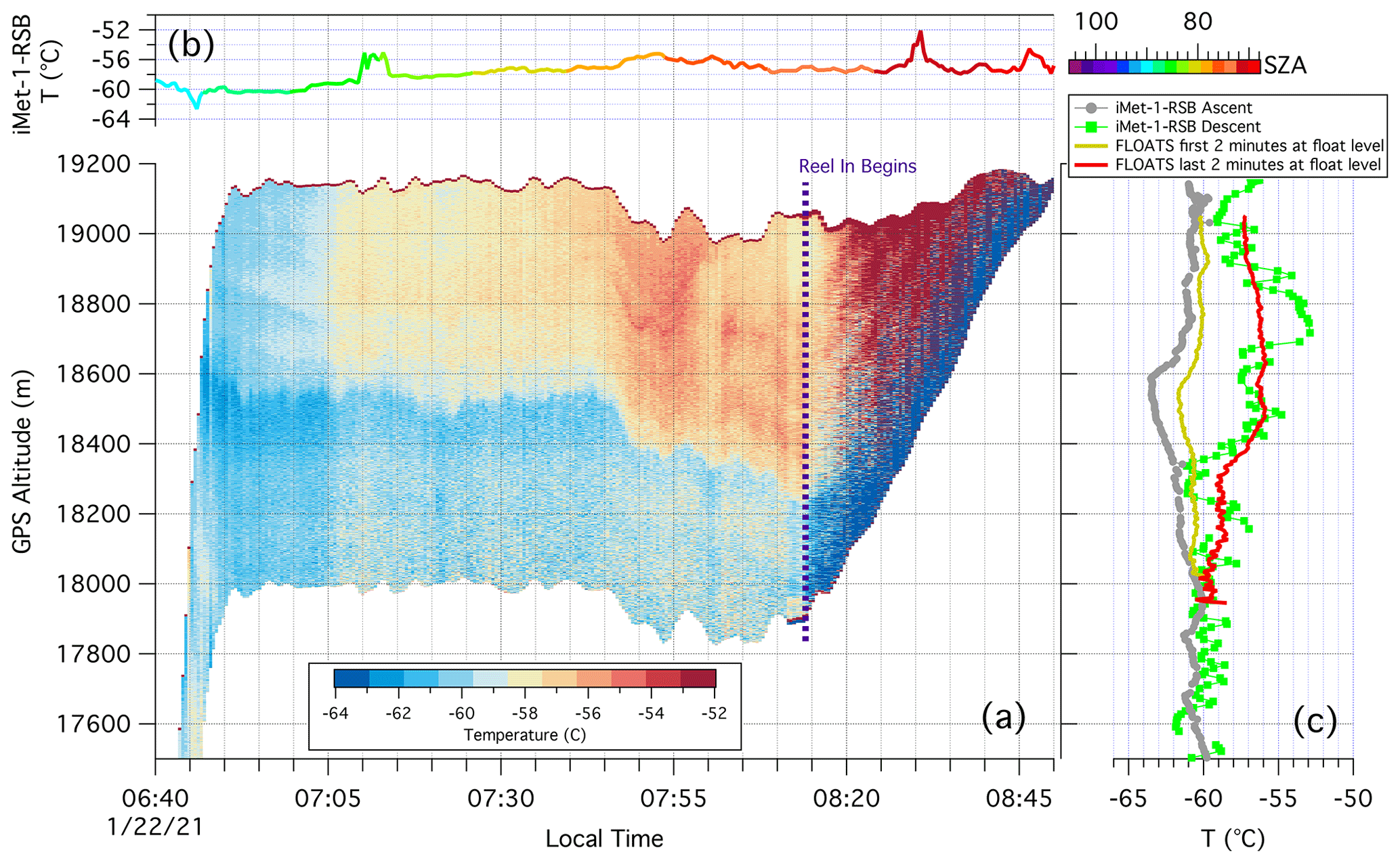
Figure 5(a) Curtain plot of DTS profile temperatures in ∘C at or near-flight altitude as a function of altitude and local time (MST). (b) Gondola-level temperature in ∘C as a function of local time and colored by the altitude-adjusted solar zenith angle. (c) The iMet-1-RSB ascent and descent temperature profiles and FLOATS average profiles in ∘C as a function of altitude. The time where the fiber-optic reel-in begins is indicated with a dashed purple line.
As shown in Fig. 5a, the fiber-optic reel-in begins at about 08:15 MST, and after that period the FLOATS temperature profiles become inconsistent compared to the previous profiles, probably because of optical distortion. Because of this distortion, the profiles from the reel-in period are excluded from any analysis and comparison to the iMet-1-RSB descent profile. The reported descent profile, however, had similar thermal structure to the FLOATS profiles from the period prior to reel-in (Fig. 5c). A narrow cold layer was seen at 18.3 km, and above 18.6 km a ∼700 m warm layer with a maximum temperature of −52.9 ∘C was reported. A comparison of the average FLOATS temperature profile 2 min prior to reel-in and the descent profile at the same altitude revealed an MAE of 1.3 ∘C. By contrast, the same FLOATS average had an MAE of 4.0 ∘C compared to the iMet-1-RSB ascent profile. The overall agreement in thermal structure between the reported ascent and descent profiles and the FLOATS profiles demonstrates that FLOATS aboard a near-constant-altitude balloon is an effective tool for understanding the evolution of vertical temperature structure at a high spatial and temporal resolution over a continuous domain.
3.5 Comparison with outside datasets
Temperature profiles from outside the WY933 flight, including COSMIC-2 (Constellation Observing System for Meteorology, Ionosphere and Climate, C2) and local meteorological soundings, are used to further evaluate the performance of FLOATS. Sounding data were retrieved from the Wyoming Upper Air website (http://weather.uwyo.edu/upperair/sounding.html, last access: 26 January 2021) for the Denver, Colorado (DNR; 72468), and the Riverton, Wyoming (RIW; 72672), stations for 22 January 2021 12:00 UTC. Level-2 AtmPrf COSMIC-2 temperature profiles for 20–24 January 2021 (UCAR Cosmic Program, 2019) were downloaded from the UCAR CDAAC website (https://data.cosmic.ucar.edu/, last access: 7 May 2021). Because of the low-inclination orbit of the COSMIC-2 constellation and subsequent sparse spatial coverage at mid-latitudes, only 58 profiles within a ±12∘ longitude and ±6∘ latitude range of WY933 were available for the 5 d period based on the perigee point of the radio occultation. Three COSMIC-2 profiles were within a 400 km radius of WY933 within 12 h of the flight. A profile located at 39.69∘ N and 106.82∘ W at 13:00 LT was the closest matching COSMIC-2 profile to WY933. Following similar methods to Alexander et al. (2008), the COSMIC-2 profiles were also used to generate a 5 d background temperature profile for a ±6∘ longitude by ±3∘ latitude grid box centered at 104∘ W and 40∘ N. The average of the 21 COSMIC-2 profiles that fit the criteria was used as the background temperature profile for the study region.
The temperature profiles from the outside datasets and the FLOATS WY933 flight can be seen in Fig. 6, where the geopotential altitudes have been converted to geometric altitude for comparison between the datasets. Generally, the FLOATS average ascent profile compared well with the sounding and best-match COSMIC-2 profile. All datasets revealed a similar broad thermal structure. The profiles exhibit a lapse rate tropopause at or near 11 km, then a temperature inversion transitioning to a negative lapse rate up to about 17 km, where there was a divergence in vertical structure. Error analysis between the FLOATS ascent profile and outside datasets produces an MAE of 1.34 ∘C for the full altitude comparison between the FLOATS and COSMIC-2 best match, 1.95 ∘C for the comparison with the RIW sounding, and 3.07 ∘C for the comparison with the DNR sounding. Based on an MAE of 3.23 ∘C between the RIW and DNR soundings, the observed error between the FLOATS ascent profile and others is reasonable based on spatial and temporal differences between the datasets.
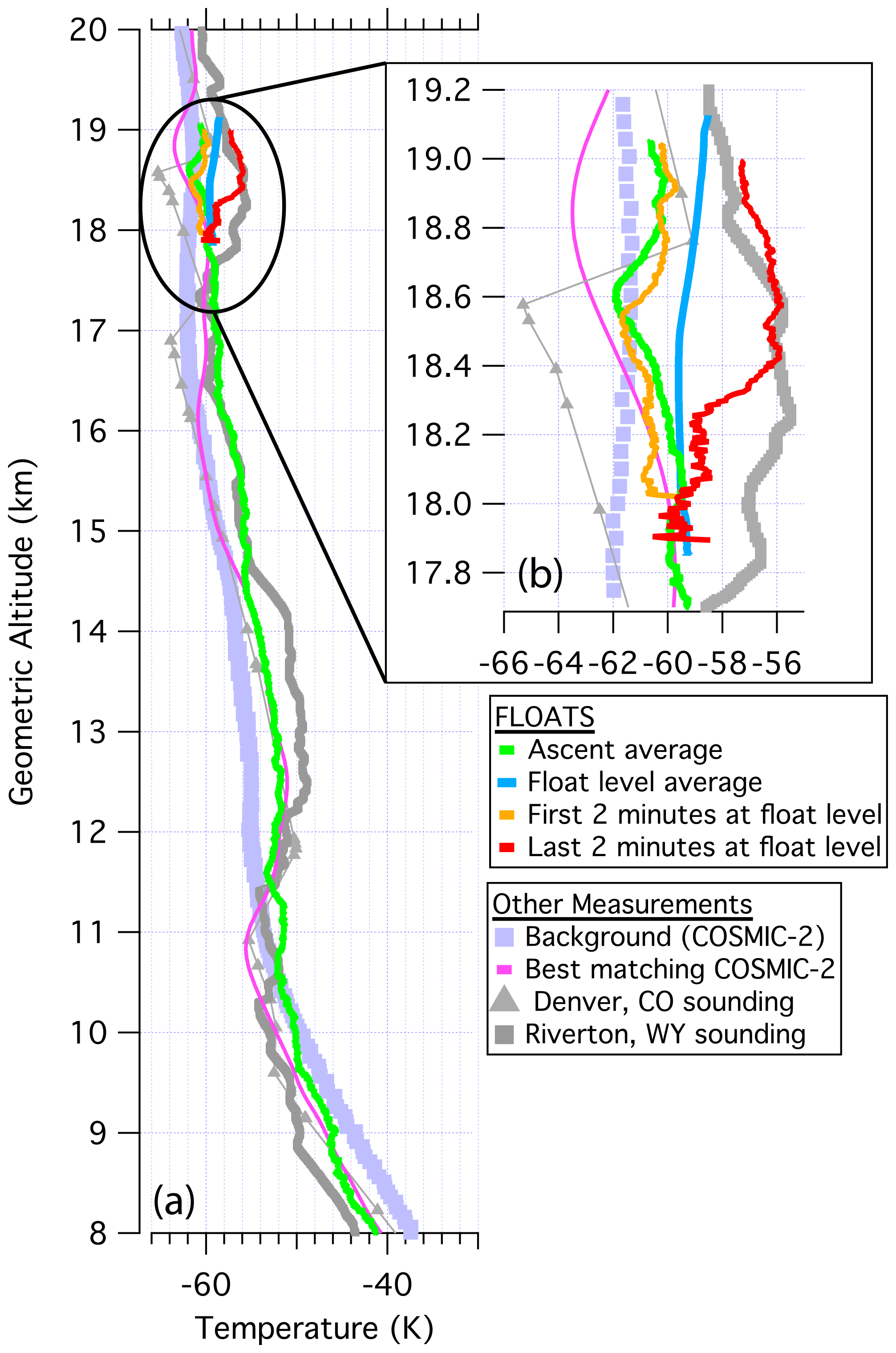
Figure 6(a) Temperature profiles in ∘C for the background temperature derived from COSMIC-2 temperature; radio sounding temperatures from Denver, Colorado (Station 72469); and Riverton, Wyoming (72672), for 22 January 2021 12:00 UTC and FLOATS DTS. The FLOATS 5 m ascent profile (green), float-level average (blue), and average temperature profiles from the beginning (orange) and end (red) of float altitude are displayed. (b) Zoomed-in section of panel (a) from 17.7 to 19.2 km altitude.
The FLOATS average temperature profile at float altitude also compared well to the outside datasets and is within a similar range of all observations (Fig. 6b). Error analysis reported an MAE of 2.40, 2.79, and 3.23 ∘C for the float-level average compared to the COSMIC-2, RIW, and DNR profiles at the same altitude, respectively. The differences between the temperature profiles appear to be related to the FLOATS profile time. The average of the first 2 min from float altitude exhibits a vertical structure similar to the DNR profile, with a cold layer near 18.5 km (Fig. 6b). On the other hand, the average of the last 2 min more closely matched the RIW profile, with a warm layer centered at the same altitude. The coincident thermal structure and range of the temperature measurements further validates the FLOATS DTS profiles and provides additional evidence for limited biassing due to solar radiative heating of the fiber-optic cable.
Finally, evaluation of the FLOATS DTS profiles compared to the COSMIC-2 background profile shows possible wave-related variability in the profiles with altitude. As seen in Fig. 6, the flight-level average suggests that WY933 was in an ∼2 ∘C warm-phase region compared to the COSMIC-2 average. Additionally, differences in the FLOATS profiles compared to COSMIC-2 were observed during different periods of flight. These comparisons suggest that FLOATS data can be used to evaluate wave-driven temperature anomalies, like those described in Kim et al. (2016) and Chang and L'Ecuyer (2020), or to evaluate small-scale energy states similarly to the methods described in Alexander et al. (2008).
3.6 Temperature anomalies and wave analysis
Here, we analyze atmospheric waves present in the FLOATS measurements. In this analysis, we will focus on two different parts of the flight: first, the balloon ascent, when the EFU underwent a series of oscillations between 06:35 and 06:50 MST; and second, when the flight was at float altitude during the period between 07:05 and 08:10 MST, when an upper-level warm layer was observed and when the balloon float level dropped vertically by ∼100 m (Fig. 5a). To provide context for the wave anomalies in the FLOATS WY933 test flight, we use the twice-daily radiosonde profiles at Riverton, Wyoming (RIW), which include T wind profiles, as well as zonal (u) and meridional (v) wind profiles. We choose a 3 d mean of these profiles to define a background that is subtracted, leaving higher-frequency sub-synoptic anomalies. The RIW sounding closest in time at 12:00 UTC on 22 January 2021 (Fig. 7a) shows stratospheric wind anomalies (u′, v′) that varied with a 3 km vertical wavelength (), with v′ phase leading ahead of u′ in altitude. These are characteristic of an upward-propagating inertia–gravity wave signal. Hodograph analysis (Hirota and Niki, 1985) of the (u′, v′) signals suggests that this is a northeastward-propagating inertia–gravity wave with intrinsic frequency (ω) of about 1.5f (where f is the Coriolis frequency) or a wave period of ∼ 11–12 h. The gravity wave dispersion relation can then be used to estimate the horizontal wavelength of ∼600 km. The wind anomalies therefore suggest a slow and large-scale wave that is likely present in both the Riverton, Wyoming, radiosonde and the WY933 balloon ascent and FLOATS profiles.
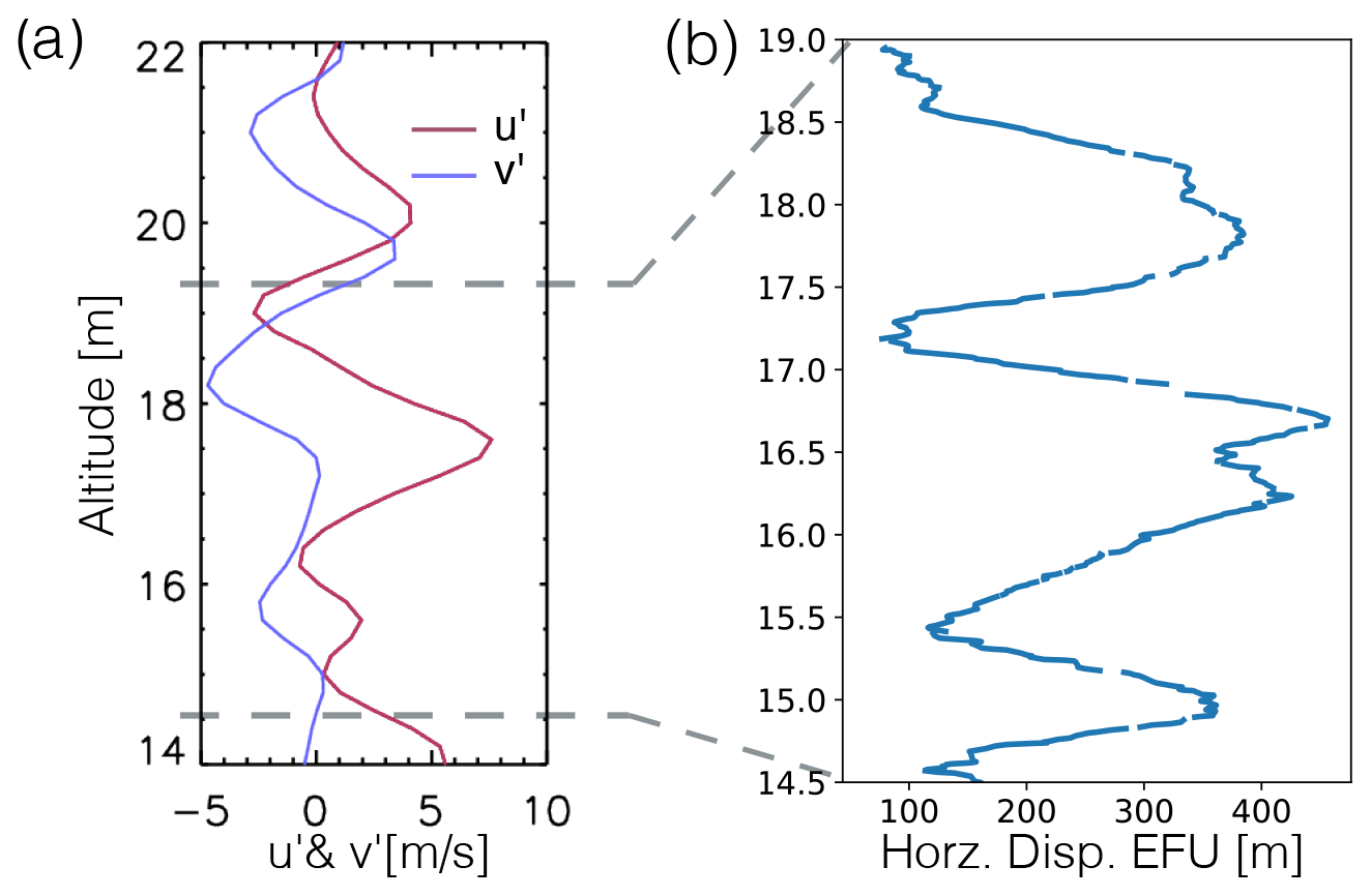
Figure 7(a) Meridional and zonal wind perturbations as a function of altitude from radiosonde observations in Riverton, WY. (b) Horizontal displacement of FLOATS EFU as function of gondola altitude.
During the ascent phase of WY933, the horizontal displacement of the EFU at the end of the 1200 m fiber length, exhibits three distinct peaks between ∼ 15–19 km (Fig. 7b). In the context of the WY933 balloon and EFU rising through the 3 km vertical-wavelength inertia–gravity wave oscillations, the peaks in the horizontal EFU displacement would occur when the wind difference between the gondola and EFU is largest. This will occur once every half cycle of the inertia–gravity wave (1.5 km), resulting in three peaks in EFU displacement as the balloon rises along the 4.5 km distance from 14.5 to 19 km. Therefore, we hypothesize that the oscillations of the EFU position are due to the vertical shear in the inertia–gravity wave.
FLOATS temperature perturbations, T′, were calculated throughout the flight as the difference between the 3 d mean T from RIW and the FLOATS profile temperature using FLOATS data binned to 1 min temporal resolution and 200 m vertical resolution to match the vertical resolution of the RIW radiosonde observations. FLOATS-measured T′ during ascent (Fig. 8a) show a warmer layer below 17 km followed by a cooler layer above 17 km. Riverton, Wyoming, sonde temperatures (Fig. 6) showed similar ±2 ∘C temperature variations but with a different phase, being cool below 17.5 km and warmer above. This is consistent with the interpretation that the same large-scale inertia–gravity wave modulates T in both locations, but the phase varies over the ∼300 km distance between the two sites.
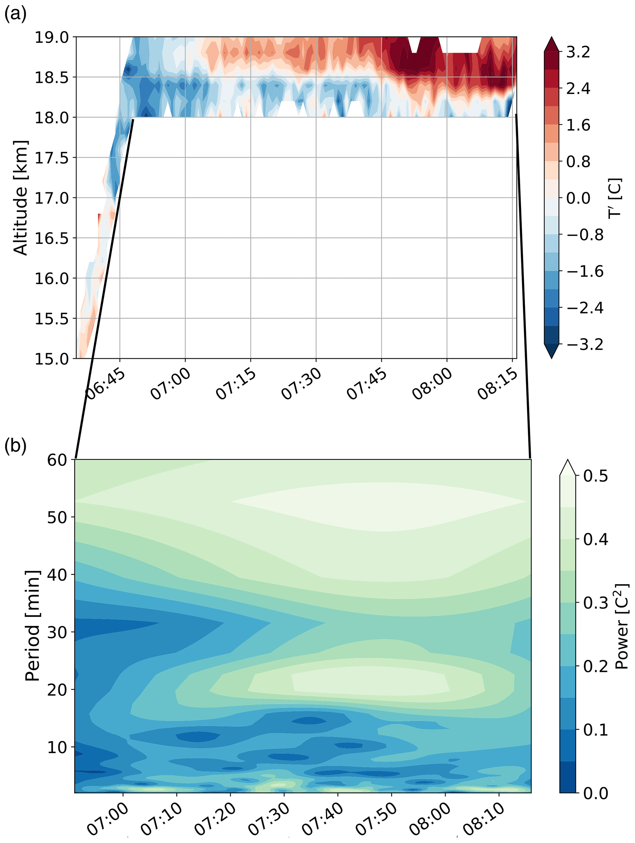
Figure 8(a) Temperature perturbations from FLOATS-observed temperature as a function of altitude and local time (MST). (b) Spectral power from FLOATS temperature perturbations as a function of wave period and local time for float-level data only.
The second period of interest of the wave analysis is characterized by an increase in temperature starting at about 07:05 MST followed by a further increase in temperature at 07:40 MST at an altitude range of 18.4 to 19.1 km (Figs. 5 and 8a). To determine if the warming layer is related to higher-frequency gravity wave activity, spectral analysis using the S transform was conducted on the T′ at the flight level (Stockwell et al., 1996), which decomposes the data in time–frequency space similarly to a wavelet transform. Frequency here is the “intrinsic frequency” in the frame of reference moving with the wind. The spectral analysis (Fig. 8b) shows enhanced spectral power >0.4 C2 for a wave period of about 55 and 20 min. This suggests that the increase in temperature at 07:05 MST can be related to the warm phase of a gravity wave with a period of 55 min and that the further increase in temperature at ∼ 07:40 MST can be related to a superposition of the 55 min period gravity wave and a gravity wave with a period of 20 min.
This analysis shows the capabilities of continuous FLOATS temperature curtain measurements to detect a variety of gravity waves with differing spatial and temporal scales. As the float time during the test flight was limited to about 2 h, the inertia–gravity wave with a period of 8 h could not be fully sampled by FLOATS. However, in future long-duration flights of up to several months (Haase et al., 2018), the ability of FLOATS to sample small vertical and temporal-scale structures will become valuable to observe both small- and large-scale waves, extending to global horizontal scales while fully resolving very short vertical wavelengths that have important effects on cirrus clouds and global circulation (Bramberger et al., 2022). These wave types are difficult to observe at the same resolution from other measurement platforms which have coarser spatial and temporal resolution. Compared to point-wise temperature sensors aboard super-pressure balloon platforms like those used in Podglajen et al. (2016), FLOATS provides temperature spectra with increased sample size, vertical displacement, and vertical resolution that can only be retrieved from continuous vertical profiling.
Fiber-optic distributed temperature sensing is an under-utilized tool for atmospheric measurements that provides low-cost and good-performance temperature measurements at spatial and temporal resolutions not possible with other sensing methods. In the tropical tropopause layer, there is a need for enhanced temperature monitoring to address questions related to vertical transport of material and atmospheric wave propagation within the region. FLOATS is a DTS system designed for up to 2 km vertical temperature profiling in the UTLS aboard drifting isopycnic balloons with a minimum sampling period of 20 s and a vertical resolution of 3 m. The instrument employs a mechanical reeling system, a self-contained end-of-fiber sub-gondola, and a four-reference temperature optical system, all designed for long-duration use within the harsh conditions of the TTL.
An experiment with the system was conducted aboard a short-duration vented balloon flight from Laramie, Wyoming, to validate FLOATS for the Stratéole 2 mission within the TTL. A major motivation for the 19 km altitude flight was to understand the technical performance of the four-reference section calibration procedure with the fiber-optic under stress loads and temperatures typical for the UTLS. Although the end-of-fiber temperature reference was damaged during launch, an adapted four-reference calibration was validated using the gondola-level temperature sensor and produced RMSE values of ≤1.4 ∘C for DTS temperatures compared to the ambient temperature sensor during the ascent phase of flight. These values show good confidence in the FLOATS measurements, considering the DTS sampling was integrated over 20 s during the ∼4 m s−1 ascent and that an error of only 0.85 ∘C was produced compared to the gondola-level temperature sensor. Evaluation with outside datasets, nearby radio soundings, and COSMIC-2 measurements demonstrate similar confidence in the FLOATS measurements. The FLOATS ascent profile was within the range of temperature profiles observed by these other platforms. Float-level temperature profiles from the validation flight demonstrate the ability of FLOATS to characterize small-scale atmospheric dynamics like gravity waves and larger-scale dynamics like inertial gravity waves at a resolution not possible with other sensing platforms. This study establishes fiber-optic distributed temperature sensing as a viable atmospheric measurement platform and FLOATS as a capable and unique balloon-borne temperature sensor for the UTLS.
To retrieve DTS temperature from the thermally complex setup of FLOATS, a two-step optimization processing scheme was developed. The method is illustrated in Fig. A1, which shows the Raman-backscattering ratio as a function of optical distance along the fiber-optic cable for a FLOATS profile from the mid-latitude flight described in Sect. 2.5 of the main text. First, the step losses due to the optical unions A and B (Fig. A1), which are positioned between reference section 1 (RS1) and reference section 2 (RS2), are assumed to be static but unique for each flight configuration. The step losses between the sections are then estimated by finding the linear fit of vs. T(z2)−T(z1) of all DTS measurements for the flight, where z1 is the furthest point of RS1 and z2 is the nearest point of RS2 with respect to the optical bench, or the nearest points to the connector, while Δα12 is the average attenuation of the two reference sections derived from the slope of ln [R(z)] as a function of distance for the two sections. The linear fit of step loss plot can then be used to extrapolate the step loss value for when the two sections and optical unions are at the same temperature (i.e., ∘C). An example of the linear fit and plotting method can be found in Fig. A2. If T(z2)−T(z1) is equal to 0 ∘C during a flight, then the from those times can be used as the primary method to retrieve the static step loss value of union A and union B for that flight or as a check of the linear extrapolation method described above. The applied step loss correction for union A and union B can be seen in Fig. A1 as the light blue ln (R) trace.
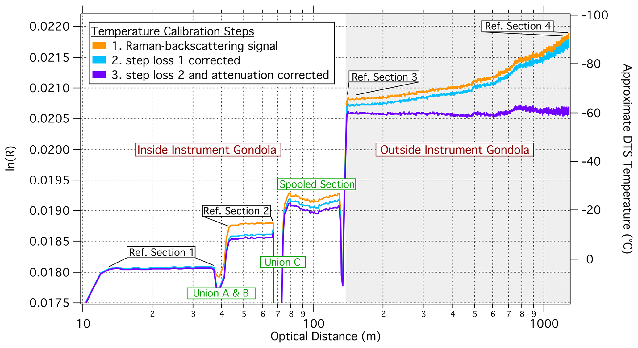
Figure A1Raman-backscattering ratio (left axis) and approximate DTS temperature (right axis) versus optical distance of FLOATS from an example profile with the full deployment of 1167 m of fiber. The raw backscattering signal (orange trace), step loss 1 corrected (blue trace), and optimized backscattering signal (purple trace) are shown. Locations of the uniform temperature reference sections are depicted with black boxes. Insertion loss and unsolvable sections are highlighted with green boxes.
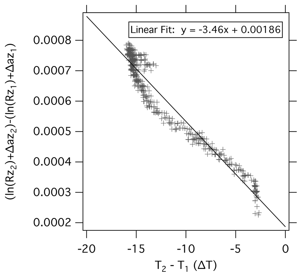
Figure A2The difference in processed Raman-backscattering signal between reference section 1 and reference section 2 from the WY933 flight versus the difference in temperature between those sections (gray crosses). The linear fit of the data is shown as a black line.
The step loss due to the fiber-optic rotary joint is more difficult to determine because that region of the instrument contains the rotary joint union, varying lengths of spooled fiber-optic cable during flight (which have uncertain micro-bend and macro-bend losses), and a large temperature transition from inside of the instrument gondola to the ambient air outside the gondola (e.g., ΔT>55 ∘C in the tropics). In Fig. A1, this region of the Raman-backscattering profile can be seen between the approximate optical distances of 65 to 110 m. The second step in the processing scheme is therefore to estimate the step loss due to the rotary joint and Δα based on a four-reference section optimization. Here we use the optimization scheme discussed in Hausner et al. (2011, Eq. 7) for each 20 s temperature profile by minimizing the absolute mean bias (MB):
where m is the number of reference sections, n is the number of DTS observations within the reference section, TDTS is the temperature at that observation point, and Tobs is the externally observed temperature for that reference section. To perform the optimization, Δα and the rotary joint step loss value (unitless) are parameterized into a range of 0.0 to m−1 and to . The TDTS is then calculated for each point along the reference section by solving for T(z) in Eq. (1) and by using Eqs. (2) and (3). The Tobs for RS3 uses the first 10 m of fiber-optic cable outside of the gondola, and Tobs for RS4 uses the 10 m of fiber-optic closest to the EFU (Figs. 1b and A1). The Tobs for RS3 is obtained from a temperature sensor outside of the gondola. The Tobs for RS4 is obtained from the EFU TSEN. An example of an optimized Raman-backscattering profile and approximate calibrated temperature can be seen as the purple trace in Fig. A1. The benefit of the described dynamic calibration scheme with parameter optimization compared to the use of static parameters is that it accounts for real time changes of the backscattering signal due to strain effects, degradation of the incident laser, or other signal aberrations that could occur during a long-duration ballooning mission like Stratéole 2.
Wind profiles from the ascent and descent phase of the WY933 flight are used to estimate the degree of ventilation along the length of FLOATS fiber-optic cable deployed beneath the flight gondola while at float altitude. Figure B1 shows the absolute value of the difference between float altitude wind speed and the wind speed at the profile position. The ascent wind difference profile is calculated with respect to the average wind speed of 8.3 m s−1 from the first 5 min at float altitude between 19.11 and 19.16 km. The descent wind profile was calculated the same way, with an average of 8.7 m s−1 from the last 5 min of flight at float altitude of approximately 19.15 km. Wind shear profiles were also calculated from the Riverton, Wyoming, and Denver, Colorado, radio soundings discussed in Sect. 3.5., with the difference based on wind speeds at ∼19.19 km. The profiles generally show wind difference values greater than 2 m s−1 from the gondola float altitude to the altitudes where the end of fiber would be located during the float phase of WY933 (i.e., between 17.8 and 18.0 km), with the exception of the first 200 m below the gondola and some sections of the FLOATS ascent and descent profiles. The low-wind-shear section in the FLOATS ascent profile between 18.0 to 18.3 km suggests that the FLOATS fiber-optic cable may have been poorly ventilated at that altitude range during the start of the float-level phase of the WY933 flight. The same low wind shear at those altitudes was not observed in the FLOATS descent profile, suggesting that the wind field was not static while FLOATS was at float level and that any poorly ventilated regions were likely not constant throughout the flight. The nearby soundings show strong and increasing wind speed with decreasing height below the WY933 float altitude, which is suggestive of synoptic-scale structure in the wind field.
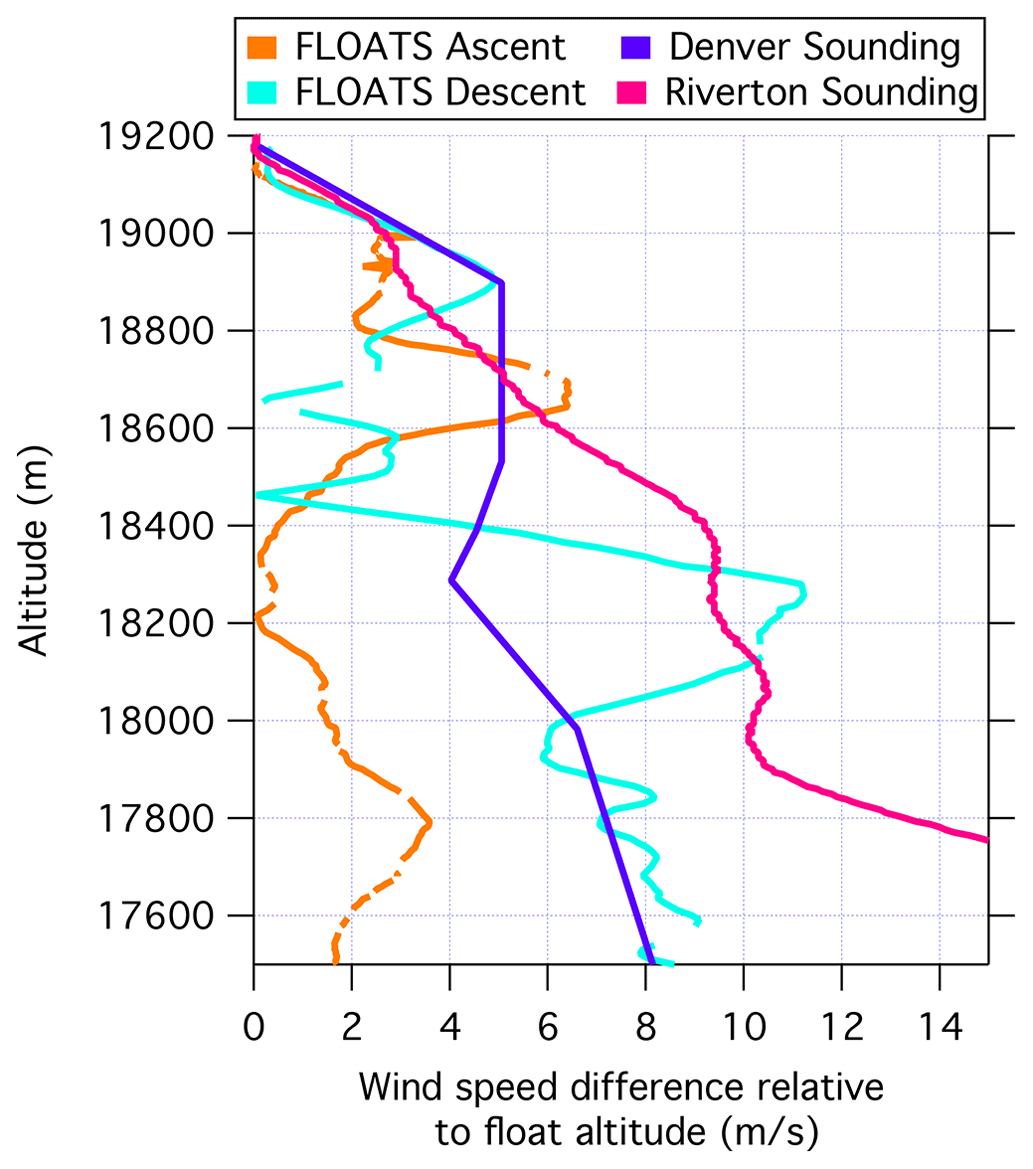
Figure B1Altitude versus the absolute value of the wind shear relative to the balloon float altitude of 19.2 km for the FLOATS ascent (orange trace) and descent phases (light blue trace) of the WY933 flight and the ascent profiles from nearby metrological soundings. The wind shear profile from the Denver, Colorado, station is shown with the purple trace, and the profile from the Riverton, Wyoming, station is shown with the pink trace. All station data are from 22 January 2021 12:00 UTC.
The data are available upon request from the corresponding author.
JDG designed and built the instrument, led laboratory testing, and drafted this paper. Early development and conceptualization of the instrument was completed by LEK, SMD, and MJA. The validation experiment was led by JDG and LEK, and the Wyoming balloon flight was headed by TD. The gravity wave analysis was conducted by MB and MJA. All authors contributed to paper editing and revisions.
The contact author has declared that none of the authors has any competing interests.
Publisher’s note: Copernicus Publications remains neutral with regard to jurisdictional claims in published maps and institutional affiliations.
We would like to thank Matt Norgren for his assistance with the Wyoming test flight. We acknowledge funding support from the National Science Foundation.
This research has been supported by the Division of Atmospheric and Geospace Sciences (nos. 1642277, 1642246, and 1642644).
This paper was edited by Ulla Wandinger and reviewed by Christoph Thomas and one anonymous referee.
Alexander, S. P., Tsuda, T., Kawatani, Y., and Takahashi, M.: Global distribution of atmospheric waves in the equatorial upper troposphere and lower stratosphere: COSMIC observations of wave mean flow interactions, J. Geophys. Res.-Atmos., 113, D24115, https://doi.org/10.1029/2008JD010039, 2008.
Bramberger, M., Alexander, M. J., Davis, S., Podglajen, A., Hertzog, A., Kalnajs, L., Deshler, T., Goetz, J. D., and Khaykin, S.: First Super-Pressure Balloon-Borne Fine-Vertical-Scale Profiles in the Upper TTL: Impacts of Atmospheric Waves on Cirrus Clouds and the QBO, Geophys. Res. Lett., 49, e2021GL097596, https://doi.org/10.1029/2021GL097596, 2022.
Chang, K.-W. and L'Ecuyer, T.: Influence of gravity wave temperature anomalies and their vertical gradients on cirrus clouds in the tropical tropopause layer – a satellite-based view, Atmos. Chem. Phys., 20, 12499–12514, https://doi.org/10.5194/acp-20-12499-2020, 2020.
de Jong, S. A. P., Slingerland, J. D., and van de Giesen, N. C.: Fiber optic distributed temperature sensing for the determination of air temperature, Atmos. Meas. Tech., 8, 335–339, https://doi.org/10.5194/amt-8-335-2015, 2015.
Drusová, S., Bakx, W., Doornenbal, P. J., Wagterveld, R. M., Bense, V. F., and Offerhaus, H. L.: Comparison of three types of fiber optic sensors for temperature monitoring in a groundwater flow simulator, Sensor. Actuat. A-Phys., 331, 112682, https://doi.org/10.1016/j.sna.2021.112682, 2021.
Egerer, U., Gottschalk, M., Siebert, H., Ehrlich, A., and Wendisch, M.: The new BELUGA setup for collocated turbulence and radiation measurements using a tethered balloon: first applications in the cloudy Arctic boundary layer, Atmos. Meas. Tech., 12, 4019–4038, https://doi.org/10.5194/amt-12-4019-2019, 2019.
Fritz, A. M., Lapo, K., Freundorfer, A., Linhardt, T., and Thomas, C. K.: Revealing the Morning Transition in the Mountain Boundary Layer Using Fiber-Optic Distributed Temperature Sensing, Geophys. Res. Lett., 48, e2020GL092238, https://doi.org/10.1029/2020GL092238, 2021.
Fueglistaler, S., Dessler, A. E., Dunkerton, T. J., Folkins, I., Fu, Q., and Mote, P. W.: Tropical tropopause layer, Rev. Geophys., 47, RG1004, https://doi.org/10.1029/2008RG000267, 2009.
Haase, J. S., Alexander, M. J., Hertzog, A., Kalnajs, L. E., Deshler, T., Davis, S. M., Plougonven, R., Cocquerez, P., and Venel, S.: Around the World in 84 Days, Eos, 99, https://doi.org/10.1029/2018EO091907, 2018.
Hanson, E. G.: Origin of temperature dependence of attenuation in optical cables, in: Optical Fiber Communication (1979), paper TuE5, Optical Fiber Communication Conference, TuE5, https://doi.org/10.1364/OFC.1979.TuE5, 1979.
Hausner, M. B., Suárez, F., Glander, K. E., Giesen, N. van de, Selker, J. S., and Tyler, S. W.: Calibrating Single-Ended Fiber-Optic Raman Spectra Distributed Temperature Sensing Data, Sensors, 11, 10859–10879, https://doi.org/10.3390/s111110859, 2011.
Henninges, J. and Masoudi, A.: Fiber-Optic Sensing in Geophysics, Temperature Measurements, in: Encyclopedia of Solid Earth Geophysics, edited by: Gupta, H. K., Springer International Publishing, Cham, 384–394, https://doi.org/10.1007/978-3-030-58631-7_281, 2021.
Hertzog, A., Basdevant, C., Vial, F., and Mechoso, C. R.: The accuracy of stratospheric analyses in the northern hemisphere inferred from long-duration balloon flights, Q. J. Roy. Meteor. Soc., 130, 607–626, https://doi.org/10.1256/qj.03.76, 2004.
Hertzog, A., Cocquerez, P., Guilbon, R., Valdivia, J.-N., Venel, S., Basdevant, C., Boccara, G., Bordereau, J., Brioit, B., Vial, F., Cardonne, A., Ravissot, A., and Schmitt, É.: Stratéole/Vorcore—Long-duration, Superpressure Balloons to Study the Antarctic Lower Stratosphere during the 2005 Winter, J. Atmos. Ocean. Tech., 24, 2048–2061, https://doi.org/10.1175/2007JTECHA948.1, 2007.
Higgins, C. W., Wing, M. G., Kelley, J., Sayde, C., Burnett, J., and Holmes, H. A.: A high resolution measurement of the morning ABL transition using distributed temperature sensing and an unmanned aircraft system, Environ. Fluid Mech., 18, 683–693, https://doi.org/10.1007/s10652-017-9569-1, 2018.
Hirota, I. and Niki, T.: A Statistical Study of Inertia-Gravity Waves in the Middle Atmosphere, J. Meteorol. Soc. Jpn., Ser. II, 63, 1055–1066, https://doi.org/10.2151/jmsj1965.63.6_1055, 1985.
Kalnajs, L. E., Davis, S. M., Goetz, J. D., Deshler, T., Khaykin, S., St. Clair, A., Hertzog, A., Bordereau, J., and Lykov, A.: A reel-down instrument system for profile measurements of water vapor, temperature, clouds, and aerosol beneath constant-altitude scientific balloons, Atmos. Meas. Tech., 14, 2635–2648, https://doi.org/10.5194/amt-14-2635-2021, 2021.
Keller, C. A., Huwald, H., Vollmer, M. K., Wenger, A., Hill, M., Parlange, M. B., and Reimann, S.: Fiber optic distributed temperature sensing for the determination of the nocturnal atmospheric boundary layer height, Atmos. Meas. Tech., 4, 143–149, https://doi.org/10.5194/amt-4-143-2011, 2011.
Khaykin, S. M., Funatsu, B. M., Hauchecorne, A., Godin-Beekmann, S., Claud, C., Keckhut, P., Pazmino, A., Gleisner, H., Nielsen, J. K., Syndergaard, S., and Lauritsen, K. B.: Postmillennium changes in stratospheric temperature consistently resolved by GPS radio occultation and AMSU observations, Geophys. Res. Lett., 44, 7510–7518, https://doi.org/10.1002/2017GL074353, 2017.
Kim, J.-E., Alexander, M. J., Bui, T. P., Dean-Day, J. M., Lawson, R. P., Woods, S., Hlavka, D., Pfister, L., and Jensen, E. J.: Ubiquitous influence of waves on tropical high cirrus clouds, Geophys. Res. Lett., 43, 5895–5901, https://doi.org/10.1002/2016GL069293, 2016.
Lagos, M., Serna, J. L., Muñoz, J. F., and Suárez, F.: Challenges in determining soil moisture and evaporation fluxes using distributed temperature sensing methods, J. Environ. Manage., 261, 110232, https://doi.org/10.1016/j.jenvman.2020.110232, 2020.
Lu, P., Lalam, N., Badar, M., Liu, B., Chorpening, B. T., Buric, M. P., and Ohodnicki, P. R.: Distributed optical fiber sensing: Review and perspective, Appl. Phys. Rev., 6, 041302, https://doi.org/10.1063/1.5113955, 2019.
Peltola, O., Lapo, K., Martinkauppi, I., O'Connor, E., Thomas, C. K., and Vesala, T.: Suitability of fibre-optic distributed temperature sensing for revealing mixing processes and higher-order moments at the forest–air interface, Atmos. Meas. Tech., 14, 2409–2427, https://doi.org/10.5194/amt-14-2409-2021, 2021.
Petrides, A. C., Huff, J., Arik, A., Giesen, N. van de, Kennedy, A. M., Thomas, C. K., and Selker, J. S.: Shade estimation over streams using distributed temperature sensing, Water Resour. Res., 47, W07601, https://doi.org/10.1029/2010WR009482, 2011.
Podglajen, A., Hertzog, A., Plougonven, R., and Legras, B.: Lagrangian temperature and vertical velocity fluctuations due to gravity waves in the lower stratosphere, Geophys. Res. Lett., 43, 3543–3553, https://doi.org/10.1002/2016GL068148, 2016.
Randel, W. J. and Jensen, E. J.: Physical processes in the tropical tropopause layer and their roles in a changing climate, Nat. Geosci., 6, 169–176, https://doi.org/10.1038/ngeo1733, 2013.
Sayde, C., Thomas, C. K., Wagner, J., and Selker, J.: High-resolution wind speed measurements using actively heated fiber optics, Geophys. Res. Lett., 42, 10064–10073, https://doi.org/10.1002/2015GL066729, 2015.
Selker, J. S., Thévenaz, L., Huwald, H., Mallet, A., Luxemburg, W., van de Giesen, N., Stejskal, M., Zeman, J., Westhoff, M., and Parlange, M. B.: Distributed fiber-optic temperature sensing for hydrologic systems, Water Resour. Res., 42, W12202, https://doi.org/10.1029/2006WR005326, 2006.
Sinnett, G., Davis, K. A., Lucas, A. J., Giddings, S. N., Reid, E., Harvey, M. E., and Stokes, I.: Distributed Temperature Sensing for Oceanographic Applications, J. Atmos. Ocean. Tech., 37, 1987–1997, https://doi.org/10.1175/JTECH-D-20-0066.1, 2020.
Stockwell, R. G., Mansinha, L., and Lowe, R. P.: Localization of the complex spectrum: the S transform, IEEE T. Signal Proces., 44, 998–1001, https://doi.org/10.1109/78.492555, 1996.
Suárez, F., Aravena, J. E., Hausner, M. B., Childress, A. E., and Tyler, S. W.: Assessment of a vertical high-resolution distributed-temperature-sensing system in a shallow thermohaline environment, Hydrol. Earth Syst. Sci., 15, 1081–1093, https://doi.org/10.5194/hess-15-1081-2011, 2011.
Thomas, C. K., Kennedy, A. M., Selker, J. S., Moretti, A., Schroth, M. H., Smoot, A. R., Tufillaro, N. B., and Zeeman, M. J.: High-Resolution Fibre-Optic Temperature Sensing: A New Tool to Study the Two-Dimensional Structure of Atmospheric Surface-Layer Flow, Bound.-Lay. Meteor., 142, 177–192, https://doi.org/10.1007/s10546-011-9672-7, 2012.
Tyler, S. W., Selker, J. S., Hausner, M. B., Hatch, C. E., Torgersen, T., Thodal, C. E., and Schladow, S. G.: Environmental temperature sensing using Raman spectra DTS fiber-optic methods, Water Resour. Res., 45, W00D23, https://doi.org/10.1029/2008WR007052, 2009.
UCAR COSMIC Program: COSMIC-2 Data Products [Level 2 atmPrf], UCAR/NCAR – COSMIC [data set], https://doi.org/10.5065/T353-C093, 2019.
van Ramshorst, J. G. V., Coenders-Gerrits, M., Schilperoort, B., van de Wiel, B. J. H., Izett, J. G., Selker, J. S., Higgins, C. W., Savenije, H. H. G., and van de Giesen, N. C.: Revisiting wind speed measurements using actively heated fiber optics: a wind tunnel study, Atmos. Meas. Tech., 13, 5423–5439, https://doi.org/10.5194/amt-13-5423-2020, 2020.
Zeidler, G., Hasselberg, A., and Schicketanz, D.: Effects of mechanically induced periodic bends on the optical loss of glass fibres, Opt. Commun., 18, 553–555, https://doi.org/10.1016/0030-4018(76)90319-9, 1976.