the Creative Commons Attribution 4.0 License.
the Creative Commons Attribution 4.0 License.
 | 28 Feb 2023
Validation of Aeolus wind profiles using ground-based lidar and radiosonde observations at Réunion island and the Observatoire de Haute-Provence
Mathieu Ratynski
Sergey Khaykin
Alain Hauchecorne
Robin Wing
Jean-Pierre Cammas
Yann Hello
Philippe Keckhut
The European Space Agency's (ESA) Aeolus satellite mission is the first Doppler wind lidar in space, operating in orbit for more than 4 years since August 2018 and providing global wind profiling throughout the entire troposphere and the lower stratosphere. The Observatoire de Haute-Provence (OHP) in southern France and the Observatoire de Physique de l'Atmosphère de La Réunion (OPAR) are equipped with ground-based Doppler Rayleigh–Mie lidars, which operate on similar principles to the Aeolus lidar and are among essential instruments within the ESA Aeolus calibration and validation (cal/val) program. This study presents the validation results of the L2B Rayleigh clear horizontal line-of-sight (HLOS) winds from September 2018 to January 2022. The point-by-point validation exercise relies on a series of validation campaigns at both observatories: AboVE (Aeolus Validation Experiment), held in September 2019 and June 2021 at OPAR and in January 2019 and December 2021 at OHP. The campaigns involved time-coordinated lidar acquisitions and radiosonde ascents collocated with the nearest Aeolus overpasses. During AboVE-2, Aeolus was operated in a campaign mode with an extended range bin setting allowing inter-comparisons up to 28.7 km. We show that this setting suffers from larger random error in the uppermost bins, exceeding the estimated error, due to lack of backscatter at high altitudes. To evaluate the long-term evolution in Aeolus wind product quality, twice-daily routine Météo-France radiosondes and regular lidar observations were used at both sites. This study evaluates the long-term evolution of the satellite performance along with punctual collocation analyses. On average, we find a systematic error (bias) of −0.92 and −0.79 m s−1 and a random error (scaled MAD) of 6.49 and 5.37 m s−1 for lidar and radiosondes, respectively.
- Article
(3176 KB) - Full-text XML
-
Supplement
(450 KB) - BibTeX
- EndNote


Wind velocity is one of the fundamental meteorological variables describing the atmospheric state. Assimilating atmospheric wind observations into numerical weather prediction (NWP) models is crucial to understand the evolution and structure of weather dynamics, air quality monitoring, forecasting, and climate and meteorological studies. Accurate NWPs are essential for commercial activities such as agriculture, fisheries, construction, transportation, energy development, and daily life. Therefore, continuous global wind profiling is essential for enhancing our understanding of atmospheric dynamics and improving the accuracy of numerical weather predictions (Houchi et al., 2010; Albertema, 2019; Stoffelen et al., 2005, 2020).
The wind measurements are conducted with a large variety of techniques: radiosondes (Houchi et al., 2010), wind profiler radars (WPRs) (Rogers et al., 1993), ground-based Doppler wind lidars (DWLs) (Chanin et al., 1989; Baumgarten, 2010; Xia et al., 2012), sodars (Anderson et al., 2005), metal resonance lidars (She et al., 2004), microwave radiometers (Rüfenacht et al., 2012), infrasound (Le Pichon et al., 2005), aircraft and airborne lidars (Prudden et al., 2018; Yan et al., 2015; Lux et al., 2020a), satellites (Eyre, 2020), and atmospheric motion vectors (Forsythe, 2007). The DWL technique offers a broad altitude range from the lower troposphere up to the lower mesosphere and a vertical resolution of around 100 m. In that sense, the Doppler wind lidars overcome most of the other instruments in terms of both vertical resolution and altitude range, making them a perfect choice as reference instruments for satellite validation. Unfortunately, there are only a handful of them being operated today.
On 22 August 2018, the European Space Agency (ESA) launched the Aeolus satellite as part of the Living Planet Programme. With an initial estimated lifetime of 3 years, this mission is expected to pave the way for future operational meteorological satellites dedicated to observing the atmospheric wind field in order to advance the understanding of climate processes and atmosphere dynamics (ESA, 2019; Straume et al., 2020). Aeolus is a polar-orbiting satellite in a sun-synchronous dawn-to-dusk orbit at about 320 km altitude.The satellite's payload consists of only one large instrument, a Doppler wind lidar called ALADIN (Atmospheric LAser Doppler INstrument), which is the first-ever Doppler Rayleigh–Mie wind lidar (DWL) in space (Stoffelen et al., 2005; Reitebuch, 2012; Kanitz et al., 2019a). ALADIN is a direct-detection high-spectral-resolution wind lidar providing vertical profiles of the horizontal line-of-sight (HLOS) wind velocity profiles at an angle of 35∘ off-nadir from the ground up to 30 km. While 30 km is the initially stated nominal range, it is very rarely used, favoring smaller ranges of observation. However, as with all satellite sensors, the remote sensing technology and retrieval algorithm require a careful assessment of the quality and validity of the generated data products. Although corrections to several substantial bias sources in the Aeolus L2B winds have been implemented in the data processing (Rennie et al., 2021; Reitebuch et al., 2020; Weiler et al., 2021b), a direct validation against high-resolution measurements is required to identify any residual biases in Aeolus' L2B winds. Total bias is a measure of the overall accuracy of a measurement, while residual bias measures the remaining error after accounting for known sources of error. Both are important in understanding the reliability and accuracy of a measurement. However, in this paper, we discuss residual bias, as it takes into account the many corrections that have been put into place in the baselines. To reflect and document changes in the baselines' residual biases, which are all merged in our large analyses, we will provide an overview of our dataset's subsets characteristics in Sect. 4.
The Aeolus Validation Experiment (AboVE) is a part of the French contribution to the Aeolus calibration and validation (cal/val) program, which included a series of intensive measurement campaigns at mid-latitude and tropical stations, Observatoire de Haute-Provence (OHP), and at the high-altitude Maido observatory at Réunion island, OPAR (Observatoire de Physique de l'Atmosphère de La Réunion). The OHP has been a historical place for lidar observations of the atmosphere for several decades (Hauchecorne and Chanin, 1980; Hauchecorne et al., 1991), while the Maido observatory saw its first observation campaigns in 2013 (Keckhut et al., 2015). Both stations are equipped with an extensive suite of lidar instruments, including Rayleigh–Mie Doppler lidars for wind profiling up to 70 km altitude using a double-edge Fabry–Pérot interferometer (direct-detection method). This technique, pioneered by French Service d'Aeronomie in 1989 (Chanin et al., 1989), is implemented in the Rayleigh channel of the Aeolus ALADIN instrument (Schillinger et al., 2003), which is why the OHP and OPAR sites are considered to be important contributors to the Aeolus cal/val program. Both AboVE-OHP and AboVE-Maido cal/val campaigns involved time-coordinated radiosounding measurements during the satellite overpass.
The paper is organized as follows: in Sect. 2, the radiosondes, the ground-based lidars, and the designs and operation principles of ALADIN are briefly described with a focus on the commonalities and differences between the two wind lidar instruments and M10 radiosondes. In Sect. 3, an overview of the two validation campaigns is given, and the procedure of matching the different resolutions of the used datasets is explained. An extensive statistical study is then proposed in Sect. 4 through a statistical comparison of entire datasets over the different regions and time periods, as well as a long-term validation over both observatories. Additionally, single case studies are presented to give further insight into the error sources. Finally, the results are discussed in Sect. 5, followed by the conclusions in Sect. 6
2.1 Experimental setup
2.1.1 Ground-based lidars
The Observatoire de Haute-Provence (OHP), located in southern France (43.9∘ N, 5.7∘ E; 683 m above sea level), is one of the Alpine stations of the Network for the Detection of Atmospheric Composition Change (NDACC). The LIOvent Doppler lidar was deployed at OHP in 1993 and provided the first lidar-based wind climatology in the middle atmosphere (Souprayen et al., 1999). The lidar senses the horizontal wind components by measuring the Doppler shift between emitted and backscattered laser light using a double-edge Fabry–Pérot interferometer, FPI (Chanin et al., 1989), which is the direct-detection technique implemented in ALADIN's Rayleigh channel. The spectral configuration of the LIOvent FPI enables sensing the Doppler shift not only in clear air but also in the presence of thin clouds or aerosol layers; however, the measurement error increases with the backscatter ratio (Souprayen et al., 1999). The Doppler shift corresponds to the projection of the horizontal wind components onto the line of sight of the laser, inclined off-zenith.
The lidar makes use of a Quanta-Ray Pro290 Q-switched, injection-seeded Nd:YAG laser emitting at 532 nm with a repetition rate of 30 Hz, 800 mJ per pulse energy. The laser beam is cycled successively between three lines of sight with a cadence of 1–2–2 min for measuring the zonal and meridional wind components, whereas the vertical pointing is used for calibration. The OHP system includes three fixed telescope subassemblies, each comprising a mosaic of four 50 cm mirrors: one is pointed toward the zenith, while the others are tilted at 40∘ off the zenith to the north and east directions. The laser beam is steered by a galvanometric scanner mirror with the three predefined positions. Measurements are limited to nighttime or twilight conditions and the absence of optically thick clouds. After a series of technical upgrades that started in 2013, the LIOvent lidar has become an operational instrument with a capacity of wind profiling up to 75 km (Khaykin et al., 2020) and was approved as a climate monitoring instrument by NDACC in 2021.
In 2012, another Doppler lidar (LiWind) was deployed at the new tropical high-altitude Maido observatory of OPAR (21∘ S, 55∘ E; 2200 m a.s.l.) on the island of Réunion. The LiWind system at OPAR uses the same laser, detection, and acquisition systems as the OHP wind lidar but features a more compact design for the receiver assembly. The telescope is made up of a single rotating 60 cm mirror, which serves for both the emission and reception (Khaykin et al., 2018). Compared to the OHP's lidar, the smaller collective area of LiWind instrument is compensated for by the station's higher elevation and the cleaner atmosphere above the Indian Ocean. Both OHP and OPAR lidars provide wind measurements with an accuracy of better than 1 m s−1 within the entire range of Aeolus altitude coverage. Both instruments will be referred to as ground-based lidar hereinafter.
2.1.2 Radiosondes
The radiosonde (RS) wind measurements, based on a simple GPS tracking of the balloon position, offer high accuracy and vertical resolution, and their inherent errors (e.g., instrument errors) are minor compared to satellite instrument errors. They are well suited to serve as a baseline dataset for the actual atmospheric state to validate the Aeolus HLOS winds. Radiosonde measurements are known to provide a solid reference against which other measurements can be validated (B. Sun et al., 2010; Krisch et al., 2017). Furthermore, radiosondes also provide guidance for observational strategies and requirements when collecting feedback from past collocations campaigns with similar instrumentation (Iwai et al., 2021; Baars et al., 2020; Martin et al., 2021). For each launch, it can be assumed that the observation errors are not correlated between the different radiosondes. It should be noted that RSs have the problem of time and space drift in measuring the vertical wind profile (Baars et al., 2020; Martin et al., 2021). The speed and direction of the horizontal wind are calculated using GPS position changes based on the Global Climate Observing System Reference. According to the GCOS Reference Upper-Air Network (GRUAN), the horizontal measurements of wind speed and direction uncertainties are assumed to be between 0.4 and 1 m s−1 for the wind velocity and 1∘ for the wind direction (Dirksen et al., 2014). While lidars sample air advected into the fixed lines of sight, radiosonde measurements are made within the local flow. Although these instruments might not sample the exact same volume of air, their measurements are proven to be highly correlated above 500 m (Kumer et al., 2014; Khaykin et al., 2020), which makes the radiosondes fully suitable for validation of ground- and space-based lidars.
The RSs at OHP and Maido sites were flown under Totex 1200 gr balloons, drifting on average 160 km for OHP and 120 km for Maido. These values are considered when computing the spatial offset (also referred to as distance to collocation) between the Aeolus and measurements, defining collocation criteria for comparisons of Aeolus and RS measurements. In this study, the RS measurements were performed with no specific spatial offset criterion in order to assess the impact of the distance to collocation on the bias and random error. The closest distance to collocation was 23 km, and the farthest was 241 km.
2.2 Aeolus ALADIN instrument
The payload of Aeolus satellite consists of a single instrument – the Atmospheric LAser Doppler INstrument. The instrument samples the atmosphere with a laser pulse and measures the resulting Doppler shift on the returned signal, resulting from the different backscatters throughout the different layers of the atmosphere. The frequency shift is caused by the relative motion of the detected elements along the sensor's line of sight. This motion is correlated to the mean wind in the observed volume. The measurement volume is determined by the vertical resolution, the width of the laser footprint, and the ground integration length. The measurements are repeated every 80 km. Each profile comprises several measurements clustered through grouping identifiers (de Kloe et al., 2016). The measurements are approximately 2.85 km (horizontal scale) apart from each other, and each of them is separately analyzed for atmospheric scene classification (Rennie and Isaksen, 2020). The along-orbit interval between individual profiles, obtained by aggregating 30 measurements to improve the signal-to-noise ratio, is ∼87 km. The measurements were classified using particle backscatter coefficients or feature lookup algorithm as criteria (Rennie et al., 2020) until 8 October 2020. Past that point, the baseline 2B11 introduced for the Rayleigh channel (the change was already in place for the Mie channel in 2B07) a different classification method, based on a signal-to-noise ratio (SNR) threshold. The Level 2B product consists of four distinct wind observation types, selected using the atmospheric classification performed in the processor chain (Rennie et al., 2020). The method currently applied by ESA is to use the Mie SNR threshold for classification of the Rayleigh channel, which is determined as part of Level 1B (L1B) processing (Reitebuch et al., 2014) and used as input for L2B processing (de Kloe et al., 2016; Rennie et al., 2020). For this purpose, a predefined SNR threshold as a function of height is used. If the SNR is greater than the threshold, the particle scattering is dominant. Under the threshold, only molecular scattering is assumed. Range bins allocated to the same classification type are accumulated in the corresponding observations. The four wind types consist of Rayleigh- and Mie-derived winds and can be either categorized clear or cloudy. The Rayleigh and Mie wind retrieval algorithms are applied to their respective two classes of observations.
Since the optimal performance of the ground-based Doppler lidars is achieved in the clear-sky conditions, this paper will only focus on the ALADIN Rayleigh clear data analysis. Rayleigh clear stands for clear skies. According to the Rayleigh approach, the winds are measured in regions showing absence of strong Mie backscatter. The presence of a high backscatter ratio would qualify the data as Rayleigh cloudy, as for cloudy/particle-loaded skies. Rayleigh cloudy products can also provide usable wind measurements. However, contamination of the Mie scattering must first be corrected, which is still in the experimental stage and is not within the scope of this study, therefore limiting our study only to the Rayleigh clear product. The Level 2B product provides an HLOS error estimation for each range bin in the observation profiles. The validity flag (de Kloe et al., 2016) ensures the validity of the products.
We also apply the quality control guidance L2B threshold from the Aeolus NWP impact experiments (Rennie and Isaksen, 2020), except we do not apply any HLOS estimated error threshold. The reason for this choice is to allow for more data to be collocated and also to observe the satellite's behavior in the higher altitudes, where is it shown to have a higher error. In this study, we present data from baselines ranging from 2B02 and from 2B11 to 2B13, covering the period from September 2018 to January 2022.
During the Aeolus commissioning phase, it was noted that pixels of ACCDs (accumulation charge-coupled devices) with an increased dark current were present in the memory zone of both ACCDs in the detector unit of ALADIN (Reitebuch et al., 2020; Kanitz et al., 2019b). These pixels are called hot pixels, and their increased dark current can have a time-variable magnitude. The results presented by Weiler et al. (2019a) revealed that by May 2020 6 % of ACCD pixels could be classified as hot pixels. Approximately 13 % of pixels will be concerned by this issue at the end of the mission's extended life in spring 2023, assuming the hot-pixel generation rate does not change (Weiler et al., 2019a). Meanwhile, a hot-pixel correction has been in place for Aeolus data since 14 June 2019. Keeping the hot-pixel appearance rate under a minimum is of the utmost importance: it can greatly affect the collocations between Aeolus and the reference instruments, making them harder to estimate the nominal behavior of the satellite (See Sect. 4.1).
The wind is observed orthogonal to the satellite ground track, pointing 35∘ off-nadir, away from the Sun (Lux et al., 2020a, their Fig. 5). (H)LOS means (horizontal) line of sight. A single wind component, called vLOS, is measured along the satellite's line of sight (LOS). The latter is then converted into the HLOS wind speed by assuming that the vertical wind speed w is negligibly small. Equations (1) and (2) allow obtaining the vLOS and HLOS based on the three Cartesian wind components u (zonal wind), v (meridional wind), and w (vertical wind). If w is assumed to be minor, the difference between vLOS and HLOS becomes proportional by a factor of cos(Ψ). The angle Ψ represents the elevation of the target-to-satellite pointing vector (55∘), and the angle θ is the topocentric azimuth of the target-to-satellite pointing vector, measured clockwise from north.
2.3 Comparison setup
2.3.1 Adaptation of the measurement grid
Two significant aspects must be considered for adequate comparison of the radiosonde wind profiles with the Aeolus wind data. First, the two instruments' different horizontal and vertical resolutions necessitate an adaptation of the radiosondes' measurement grid to that of Aeolus. Aeolus' data format consists of 24 vertical range bins that divide the atmosphere, resulting in wind profiles that can be obtained between 0 and 30 km, displaying a vertical resolution between 250 and 2 km (Reitebuch et al., 2014). The distribution of these 24 range bins is defined through a dedicated range bin setting (RBS). The main reason for adding or changing a RBS is to address a specific need, such as better sampling at specific heights. The RBS can therefore vary depending on the latitude and the time, which is all adjusted operationally. In this study, we operate with the bins of varying sizes (from 500 to 1500 m) and a vertical range from the ground up to a maximum altitude (varying between 17.8 and 28.7 km). The radiosonde data have a vertical range up to 35 km, depending on the balloon burst altitude, and the vertical resolution is approximately 5 m at the typical rate of climb of 5 m s−1. The ground-based lidars have a vertical range of up to 75 km and a resolution of 120 m.
Since the instruments have around 5000 measurement points for the radiosondes down to 200 measurements points for the ground-based lidars, compared to the satellite's 24 (at best, if all the measurements have passed quality checks) measurements for a single profile, a downsampling of these two reference datasets is required. Each Aeolus profile is used as a reference for the collocated profiles downsampling, meaning that the averaging grid is specific to each satellite observation. In order to match the resolution of the Aeolus measurements, we first average the reference measurements between the bounds of each Aeolus bin. This avoids the need for interpolation and ensures that the reference measurements are at the same resolution as the Aeolus measurements. The result will be a reference profile downsampled to the corresponding numbers of Aeolus bins present in the profile (∼21 on average, when considering the validity flags).
2.3.2 Consideration of the different viewing geometries
The second significant aspect to consider when comparing different instruments is the different viewing geometries. Because Aeolus only measures in one direction, it is necessary for the other two instruments, the ground-based lidars and the radiosondes, to project their measurements onto the same line of sight. The HLOS wind component is computed as a linear function of the zonal wind component u and the meridional wind component v using Eq. (2), where θ (259.9∘100∘ for OHP and 259.0∘101∘ for Maido, for ascending/descending orbits) is the topocentric azimuth angle, which is defined clockwise from north of the horizontal projection of the target to the satellite pointing vector. Therefore, each observation site has its own azimuth angle value.
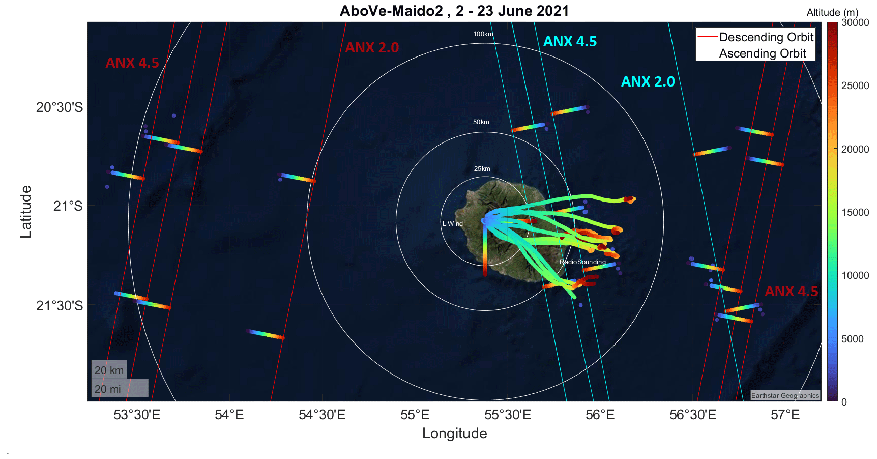
Figure 1AboVE-Maido-2 campaign overview with ascending and descending Aeolus overpasses in cyan and red. The colored trajectories represent the ascending phase of the radiosondes, with their altitude shown through a color map. The straight colored strokes represent lidar measurements from Aeolus and the ground-based lidar. The ascending node crossing configuration is specified for each Aeolus overpass. Credit: base map source is Earthstar Geographics.
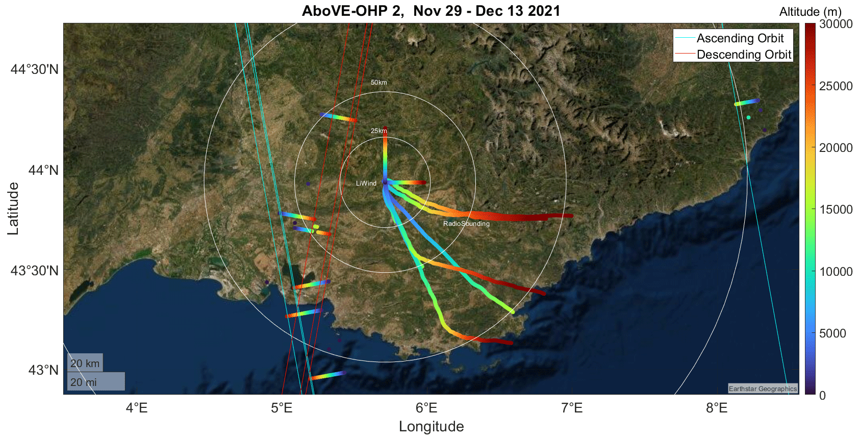
Figure 2AboVE-OHP-2 campaign overview with ascending and descending overpasses in cyan and red. The colored trajectories represent the ascending phase of the radiosondes, with their altitude shown through a color map. The straight colored strokes represent lidar measurements from Aeolus and the ground-based lidar. Credit: base map source is Earthstar Geographics.
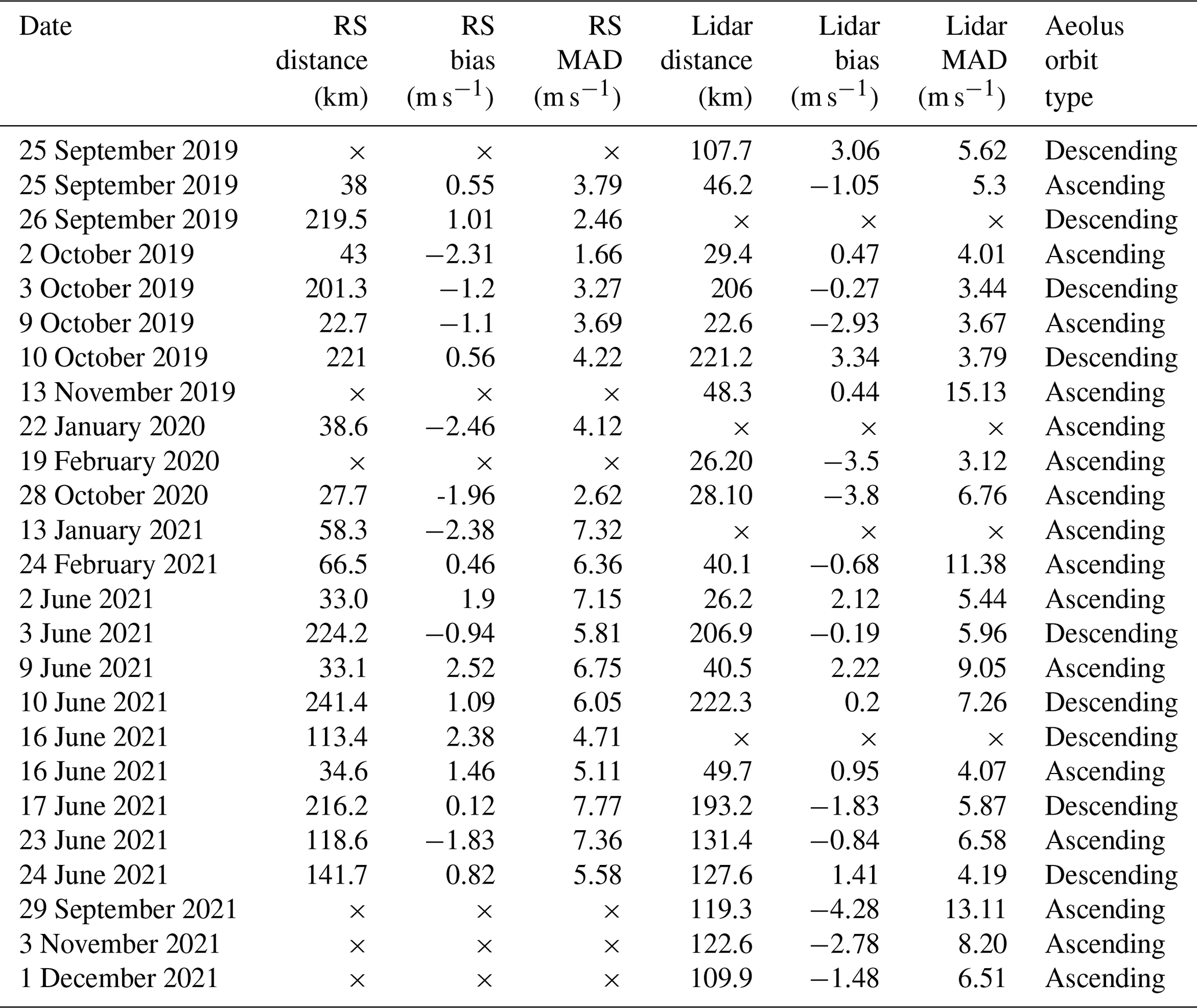
Table 1Overview of the complete list of AboVE-Maido-1 and 2 Aeolus overpass collocations. The cases of single collocations are also included. The distance is calculated over the average position of each instrument. A more detailed table is provided in the Supplement.
2.3.3 Statistical terms and methods
The offset between Aeolus and the reference data, also referred to as bias, representing the systematic error of the Aeolus wind measurements, is studied alongside the scaled median absolute deviation (MAD), representing the random error. The MAD is preferable to the standard deviation because it is less sensitive to outliers (Ruppert, 2011). We refer to the scaled MAD as a random error. The standard deviation is also used in specific cases. The bias, standard deviation, and scaled MAD are calculated as
where 1.4826 represents the scale factor, i the index, and N the number of samples. Pearson's correlation coefficient, R, between the HLOS Aeolus wind component and the HLOS instrument component sample is calculated using Eq. (6), where xi and yi represent the sample i point of Aeolus and the instrument, respectively. and represent the mean wind component of the datasets.
The scaled MAD is identical to the standard deviation (Eq. 4) if the analyzed data follow a normal distribution. In addition to the metrics presented above, a least-square line fit to the respective datasets is performed to also provide the slope and the approximated bias, which we refer to as the intercept.
3.1 AboVE Maido
The AboVE-Maido campaigns took place from 25 September to 10 October 2019 (AboVE Maido 1) and from 31 May to 24 June 2021 (AboVE Maido 2). Eleven additional measurements were conducted outside the campaign's dates. The campaigns took place at the high-altitude Maido observatory on the French island of Réunion. Calibration and validation activities at the observatory included Doppler Rayleigh lidar operation, ranging from early night measurements to dusk-to-dawn observations (depending on the overpass's time), to cover both ascending and descending orbits as well as time-coordinated radiosondes ascents during and in between the overpasses. The ANX, or ascending node crossing, is the point where the orbit of Aeolus intersects the x–y plane in the Earth's fixed coordinate system. During the campaign, the orbit parameter for the ANX was changed from ANX 4.5 to ANX 2.0 (as shown in Fig. 1) to support the Aeolus tropical campaign activities in Cabo Verde. This change resulted in a shift in the orbit's location relative to the observatory. Previously, the ANX 4.5 ascending orbit was located within 10 km of the lidar's eastward line of sight in the lower stratosphere on Wednesdays. After this change, the ascending orbit moved further away from the lidar's eastward line of sight but remained within a distance of 200 km.
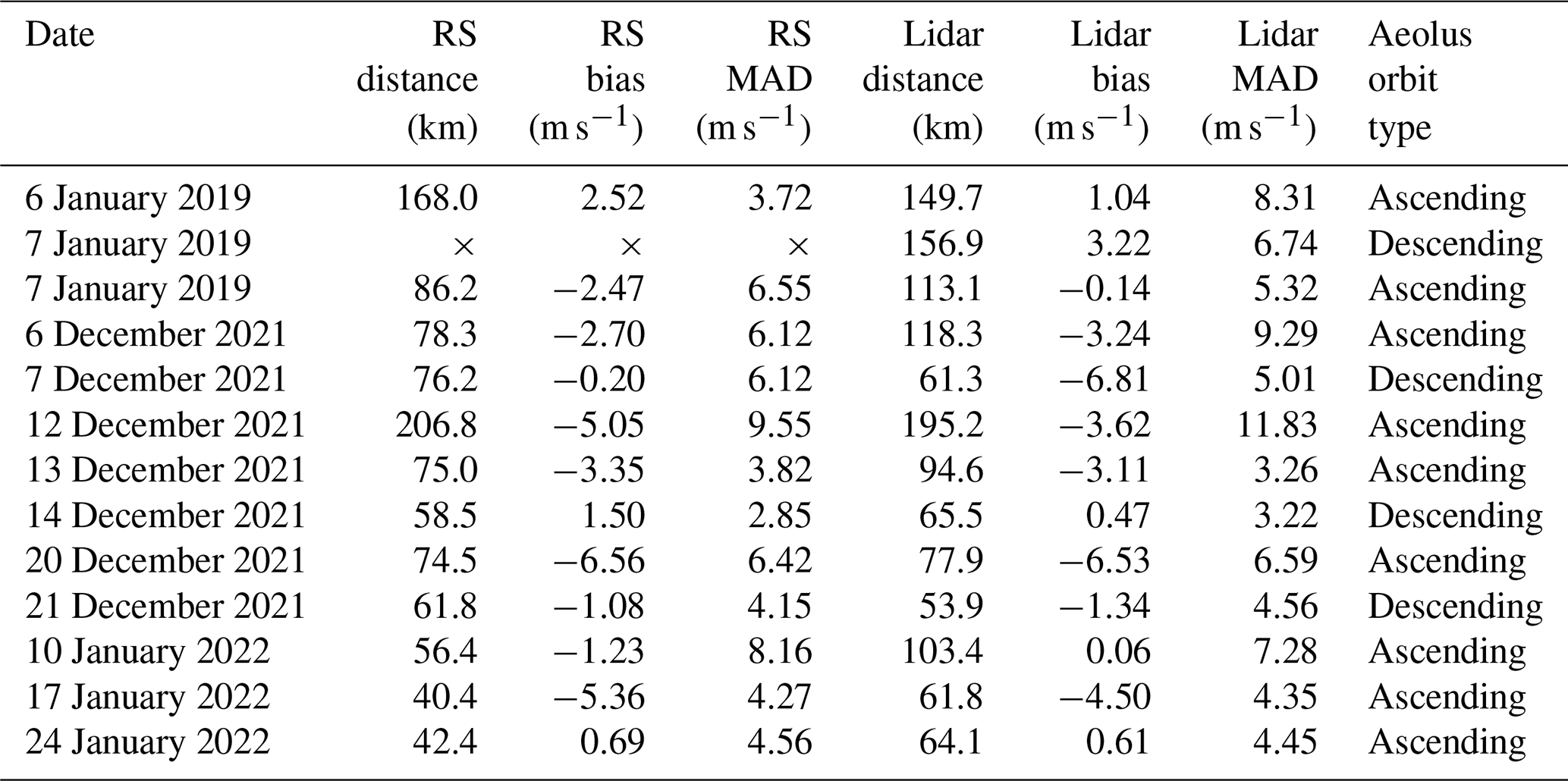
Table 2Overview of the complete list of AboVE-OHP-1 and 2 Aeolus overpass collocations. The distance is calculated over the average position of each instrument. A more detailed table is available in the Supplement.
Thanks to coordination with ESA, the AboVE-Maido-2 campaign took advantage of specific settings planned in advance. A particularity of this campaign is its unique range bin setting: the Réunion RBS. This specific setting raises Aeolus' top altitude to 28.7 km, which permits intercomparisons higher into the stratosphere. This increase in vertical range is possible at the expense of the resolution (see Sect. 2.3). It is only activated when the satellite overpasses the vicinity of the island. After the AboVE2-Maido campaign, the cal/val measurement sessions at Maido were conducted once per month until the end of 2021. The OPAR lidar lines of sight facing east, south, and zenith are shown in Fig. 1. The eastward line of sight is such that the lidar acquisition area is crossing with that of Aeolus in the stratosphere (around 40 km altitude), reducing the influence of the spatial offset. The minimum spatial offset between Aeolus ascending phase and reference measurements was 22.1 and 22.6 km for the lidar and radiosondes, respectively. At the same time, the descending Aeolus orbits were much further away, with the spatial offset ranging from 54 to 241.4 km. During both campaigns, 19 Aeolus-collocated RS ascents were carried out, and 15 were time-coordinated with ground-based lidar acquisitions. The baseline, date, distance to collocation, bias, standard deviation, and scaled MAD for both reference instruments, Aeolus overpass time, and orbit type are provided in Table 1.
3.2 AboVE OHP
The AboVE-OHP campaigns took place from 6 to 14 January 2019 (AboVE OHP 1) and from 29 November to 14 December 2021 (AboVE OHP 2). Additional measurements were conducted on 20 and 21 December 2021 and 10, 17, and 24 January 2022. The ANX 4.5 orbit, active during AboVE OHP 1, allowed for collocations with both ascending and descending orbits, within 100 to 150 km. The AboVE2-OHP benefited from the satellite orbit modification: the ANX 2.0 orbit enables collocations within 50 km twice per week for ascending and descending orbits as seen in Fig. 2. Similar to the AboVE-Maido-2 campaign, the measurements included dusk-to-dawn coverage, shorter measurements, and radiosondes ascents. The satellite's AboVE2-OHP range bin setting is the same as the AboVE-Maido-2 RBS, since the goal is to compare the two regions' datasets and differentiate biases between the ones inherent to the setting and the ones due to the geographical location.
4.1 Statistical comparison of Aeolus with collocated data
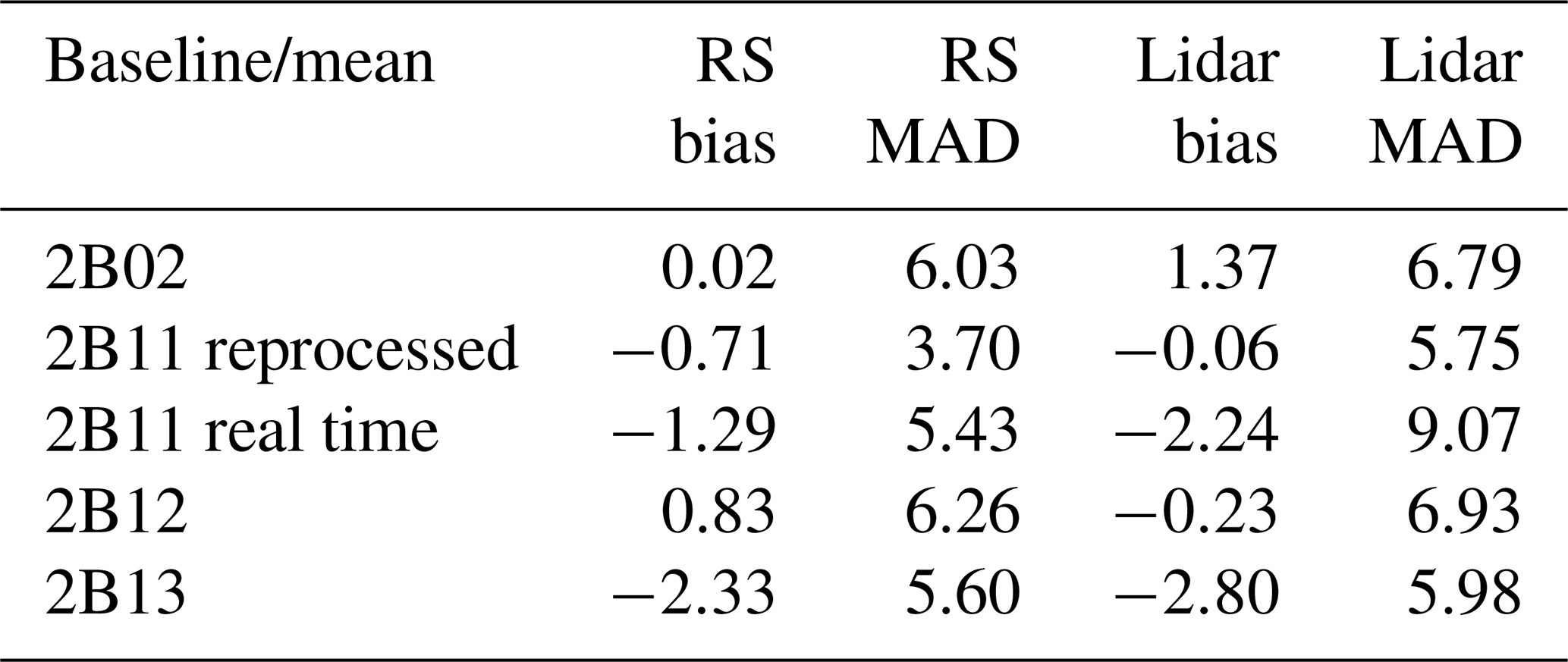
In this subsection, we statistically analyze the comparisons before discussing Aeolus' capacities and performance at different altitudes. The dataset presented consists of the combined measurements from both cal/val sites, including all time periods. For this analysis, we will study the mean bias as a function of altitude, along with the number of collocated data points in Fig. 3. Additionally, we will present the Aeolus Rayleigh wind values plotted in Fig. 4 against the corresponding values of the reference instruments downsampled to match the Aeolus height resolution (as discussed in Sect. 2.3). We provide an overview of all the validation cases in Tables 1 and 2. Concerning the two reference instruments, a point-by-point comparison shows a mean bias of 0.1 m s−1 between the wind profile of the lidar and that of the radiosonde, with a standard deviation of 2.3 m s−1. The Aeolus instrument settings and ground processing have significantly changed during its mission. These will affect statistical properties like bias and standard deviation/MAD. In addition to the combined statistics, we provide in Table 3 a splitting of the results, presenting them separately for the different baselines. Also, near-real-time and reprocessing results are separated, i.e., baseline 11 (introduced in near-real-time processing on 8 October 2020) and the baseline 11 results before that date (based on reprocessed Aeolus data). The split is needed since the reprocessing used different calibration data than the near-real-time processing, along with several changes in the correction. The main refinements in the reprocessed dataset are improvements in the hot-pixel correction by a more careful application of the method, along with using the data of the day itself rather than the day before for the M1 telescope temperature correction. The newer baseline should expect improved overall and local biases (ESA, 2021b).
Table 3Overview of the different characteristics (Bias and MAD) averaged (mean) for each instrument and baseline. The real-time and reprocessed data are also separated because of varying calibration parameters.
Within the dataset, distances to collocation vary between 22.1 and 207 km for ascending orbits and between 54 and 241.4 km for descending orbits. Therefore, the spatial offsets are highly variable, depending on the orbit phase and the ascending node crossing (ANX) setting: for ascending orbits, the average distance to collocation is 67.4 km for radiosondes and 79.1 km for lidars, whereas for descending orbits, the averages are 161.4 and 147.5 km, respectively. Such a difference does not allow for comparing the whole dataset as a unified set of collocations. The reference measurements were separated into ascending and descending orbital phases to account for that disparity.
Figure 3a and b show the mean bias as a function of altitude, with the shading representing the standard deviation. From 5 km to approximately 22 km, the bias lies within the ±5 m s−1 range but increases as soon as the upper bins mark is reached. The data below 5 km have a larger standard deviation, which is consistent with what Guo et al. (2021) reports on the increased wind speed differences in the 2–3 km range for descending orbits. The same calculations were then realized, only this time within the 5–22 km window (we refer to it as the “altitude range method”). The results show that removing the higher bins decreases the random error from 5.58 to 5.38 m s−1 for ascending profiles and from 4.99 to 4.77 m s−1 for descending profiles. One other method also considered was to average every Aeolus profile within a window of 200 km around the observatory for each collocation, aggregating two or three profiles on average (we refer to it as the “average method”). With this averaging method, the random error decreases from 5.58 to 3.67 m s−1 for ascending profiles and from 4.99 to 3.38 m s−1 on descending profiles. The larger standard deviation in the lower troposphere might be due to several reasons. First, the satellite's lidar performance is largely limited by received power; therefore, the strong aerosol scattering in the boundary layer height will lower the apparent molecular scattering signal, reducing the inversion accuracy of HLOS wind from Aeolus (Tan et al., 2017). Secondly, there is also a smaller sample studied in that altitude region, which leads to an undersampling bias. The AboVE-OHP-2 lidar measurements were the only ones that had extended coverage below 5 km, which significantly reduced the number of data points in the lower troposphere.
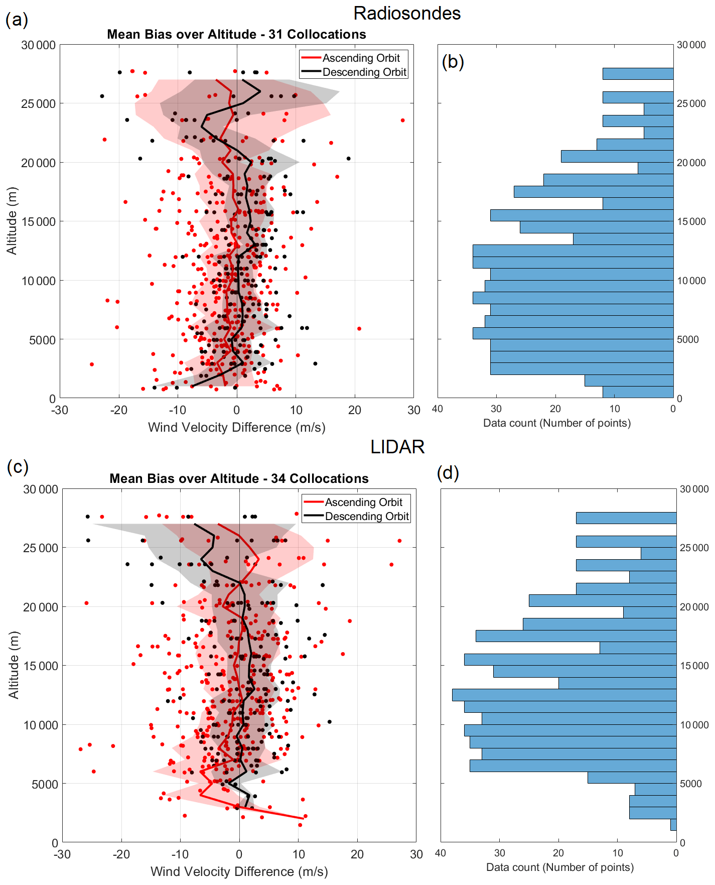
Figure 3(a) The Aeolus minus the radiosonde HLOS wind difference made during all AboVE campaigns over each altitude bin. (b) The number of data samples over each altitude bin for the radiosonde comparison. (c) The Aeolus minus the lidar HLOS wind difference made during all the campaigns over each altitude bin. (d) The number of data samples over each altitude bin for the lidar comparison. Red represents measurements of an ascending orbit, while black represents measurements of a descending orbit. The lines represent the average bias of each bin altitude, and the red (black) shading is the standard deviation of the bias in each range bin for ascending (descending) orbits.
The same observations still hold true for Fig. 3c and d, depicting the same increase in variance in the uppermost bins. Similarly, from 5 to around 22 km, the bias fluctuates within the ±5 m s−1 range, and the uppermost bins display similar features in terms of magnitude to the radiosonde's counterpart. The results differ slightly from the radiosonde observations, particularly when applying the methods of altitude range or average on the descending orbit collocations. Indeed, removing the higher bins or averaging them decreases the random error from 7.17 to 6.49 or 4.9 m s−1 (for removing the higher and lower bins or averaging several profiles together, respectively) for ascending profiles. This observation also holds for descending profiles, where the random error varies from 7.17 to 6.49 m s−1 using the altitude range method and decreases to 3.96 m s−1 with the averaging method. The result of these different methods over the various parameters is reported in Table 5. Ground-based lidar comparisons suffer from a higher random error than their radiosondes counterparts. The ground-based lidars show a higher random error in the uppermost bins because its precision decreases with air density (Khaykin et al., 2020). The lack of data points in the 26–27 km range is a specificity of the range bin setting, being the result of a compromise between height coverage and sample spacing.
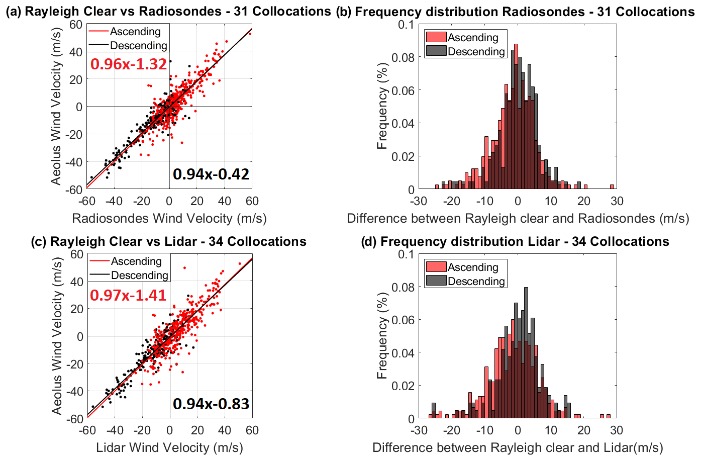
Figure 4(a) The Aeolus winds versus the radiosonde measurements made during all the campaigns. (b) Frequency distribution of the difference between Aeolus and radiosonde wind speeds for the same dataset. Red represents measurements of an ascending orbit, while black represents measurements of a descending orbit. (c) The L2B Rayleigh clear winds versus the lidar measurements made during all the campaigns. (d) Frequency distribution of the difference between Aeolus and lidar wind speeds for the same dataset. Red represents measurements of an ascending orbit, while black represents measurements of a descending orbit.
The various colors indicate if Aeolus had an ascending (red) or descending (black) node, i.e., if it was done in the evening or in the morning (local time), respectively. This separation between orbital phases is done because of the aforementioned distance to collocation disparities. Nonetheless, several long-term cal/val activities showed significant phase-dependent differences in the determined biases of Aeolus wind measurements (Wu et al., 2022; Iwai et al., 2021; Lux et al., 2021; Baars et al., 2020; Rennie and Isaksen, 2020; Krisch and the Aeolus DISC, 2020), further assessing the need for an independent study on both cases. The correlation plot of the Aeolus wind is shown in Fig. 4a, alongside the retrieved linear regression. A linear trend is clearly seen between the Aeolus and the reference radiosonde observations. The following coefficients are presented with confidence bounds of 1 sigma. The Fig. 4a ascending trend line has a slope of 0.96±0.0 with an intercept (i.e., an approximated bias) of m s−1, whereas the descending trend line has a slope of 0.94±0.03 and an intercept of m s−1. The slopes are statistically similar, but the intercepts are not. Comparing this result with radiosondes from other cal/val campaigns, Iwai et al. (2021) found a slope of 1.01 and an intercept of 0.38 m s−1 in Okinawa. Baars et al. (2020) presents a slope of 0.97, which is consistent with our observations, and an intercept of 1.57 m s−1 that could be explained by the lower maximum height of comparison, where we see the biggest shift towards negative biases (Fig. 3).
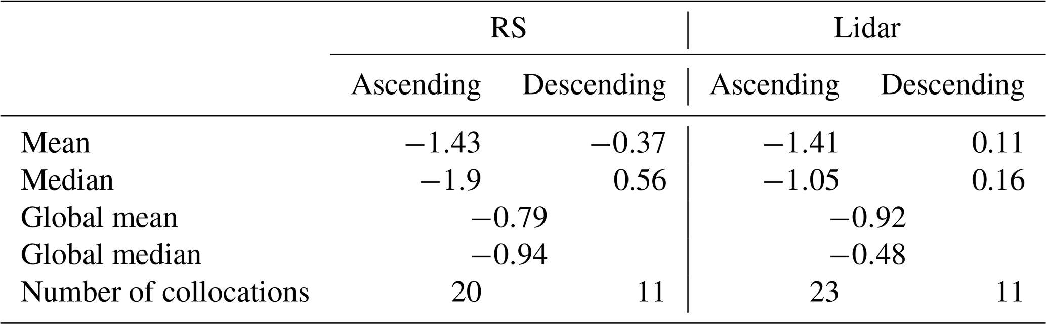
Because of its similar location and window of acquisition, the lidar data share a lot of similar conclusions. In Fig. 4c, the ascending trend line has a slope of 0.97±0.03 with an intercept of m s−1, whereas the descending trend line has a slope of 0.94±0.04 and an intercept of m s−1. The slopes are statistically similar – same as for the intercepts. Comparing these results with other cal/val studies using lidar data, Wu et al. (2022) found overall negative biases with a slope of 1 and an intercept of −0.12 m s−1, confirming the negative intercept we observe for all scenarios. Chen et al. (2022) found slopes of 0.94 and 1.02 and intercepts of −0.89 and 0.4 m s−1 for the lidar large and small geographical range, respectively. Iwai et al. (2020) found slopes of 0.98 and 1.03 and intercepts of −0.88 and −0.52 m s−1 for the Kobe and Okinawa stations respectively. Further detail on the results of Aeolus cal/val statistics (including the slope, intercept, bias, scaled MAD, standard deviation, and correlation coefficient) from various campaigns can be found in Table 7. Figure 4b shows the normalized frequency distribution of the deviation between the Rayleigh clear and radiosonde wind observations. The distribution follows a Gaussian pattern, meaning that, according to the normal distribution law, almost 70 % of the samples are within the 10 m s−1 absolute error margin. It also seems that the probability of overestimating or underestimating the wind product by Aeolus is equiprobable. When calculating the mean value of this distribution, one gets −0.79 m s−1 as the bias for the Rayleigh wind observations. If one uses the median of the distribution for the bias calculation, one gets a bias of −0.94 m s−1, which is a little more than the result calculated from the mean. All these results are reported in Table 4. The slope is close to 1 for both cases, which means that Aeolus excels at resolving wind speed variations, even if a special sparser RBS is used. Figure 4d depicts the normalized frequency distribution of the deviation between Aeolus and lidar wind observations. When calculating this distribution's average value for ascending orbit collocations (descending orbit collocations), one gets −1.41 m s−1 (0.11 m s−1) as the bias for the Rayleigh clear wind observations. If we use the median of the distribution for the bias calculation, one gets a bias of −1.05 m s−1 (0.16 m s−1). Putting these two together, the mean value becomes −0.92 m s−1 and the median −0.48 m s−1. While close, there is a clear difference in biases based on whether it is using an ascending or descending orbit in reference, further assessing the need to distinguish both cases.
Table 4Overview of the different statistics regarding the biases in Aeolus with respect to the reference instruments. The data used include all the collocations listed in Tables 1 and 2.
Overall, there is not a better slope or a lower bias for ascending orbits, which would go with the conclusion of the absence of any representative statistical difference presented by Guo et al. (2021). The data even suggest that the bias is lower for descending orbits, which would contradict the fact that they have a larger spatial offset from the reference measurement locations. We can also observe a negative bias for all the comparisons using the standard all-data method. This means that the satellite is prone to underestimating the HLOS wind speeds. A previous study indicates differences in the biases between the ascending and descending orbit phases, mainly occurring for the Rayleigh channel in late summer and autumn (Martin et al., 2021). One reason Sun et al. (2014) raised may be that the meteorological conditions such as wind speeds, boundary layer height, air temperature, and aerosol distributions differ from one orbital phase to the other. However, none of these orbit-dependent events were observed during our measurements. In addition, Weiler et al. (2021b) showed that an important contribution for orbital phase biases is the telescope temperature effect. Other studies indicate lidar comparison biases of 1.05 and −0.35 m s−1 for Chen et al. (2022), −0.13 m s−1 for Wu et al. (2021), and −0.81–0.48 m s−1 in Kobe and Okinawa respectively for Iwai et al. (2021). For radiosonde comparison biases, we observe 2.12 m s−1 from Martin et al. (2021), 1.52 m s−1 from Baars et al. (2020), and 0.45 m s−1 from Iwai et al. (2021). While the lidar comparisons biases are in good agreement with what we observe, the radiosonde biases show a greater variety in the outcomes, which might be due to the pendulum-line motion of the suspended radiosonde during the early stage of ascent (Kumer et al., 2014).
Table 5Overview of the different comparison method and their relative outcome on the statistical metrics, depending on the instrument and the orbit phase. The data used include all the collocations shown in Tables 1 and 2.
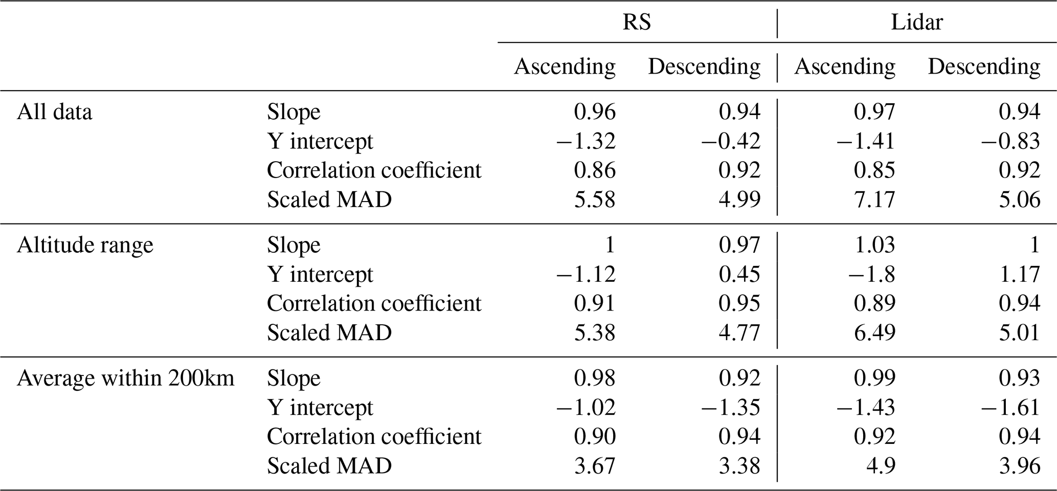
Table 5 shows the previously mentioned data and the different methods for comparison. The all-data method means that the instrument is collocated within the closest overall Aeolus overpass. The altitude range method cuts the data outside the 5 to 22 km range to account for possible RBS issues and non-optimal satellite coverage area. The last method aggregates every eligible profile (within the last 2 h) into one, averaged, single collocation. The goal was to see if the uppermost-bin issue would become insignificant after a certain amount of averaging, hence making the 22+ km range data available for usage. So far, both methods show encouraging data, reducing the scaled MAD for both instruments at any orbit type. Putting these numbers into perspective, for the radiosondes, a scaled MAD of 4.84 m s−1 is found by Baars et al. (2020), 3.97 m s−1 for Iwai et al. (2021), and 5.01 m s−1 for Martin et al. (2021). A standard deviation of 4.43 m s−1 (Iwai et al., 2021) is also reported. We report a scaled MAD of 5.37 m s−1 and a SD of 6.18 m s−1, which belongs to the same range of results, if we account for the fact that we consider a broader altitude range for comparison (see Table 5).
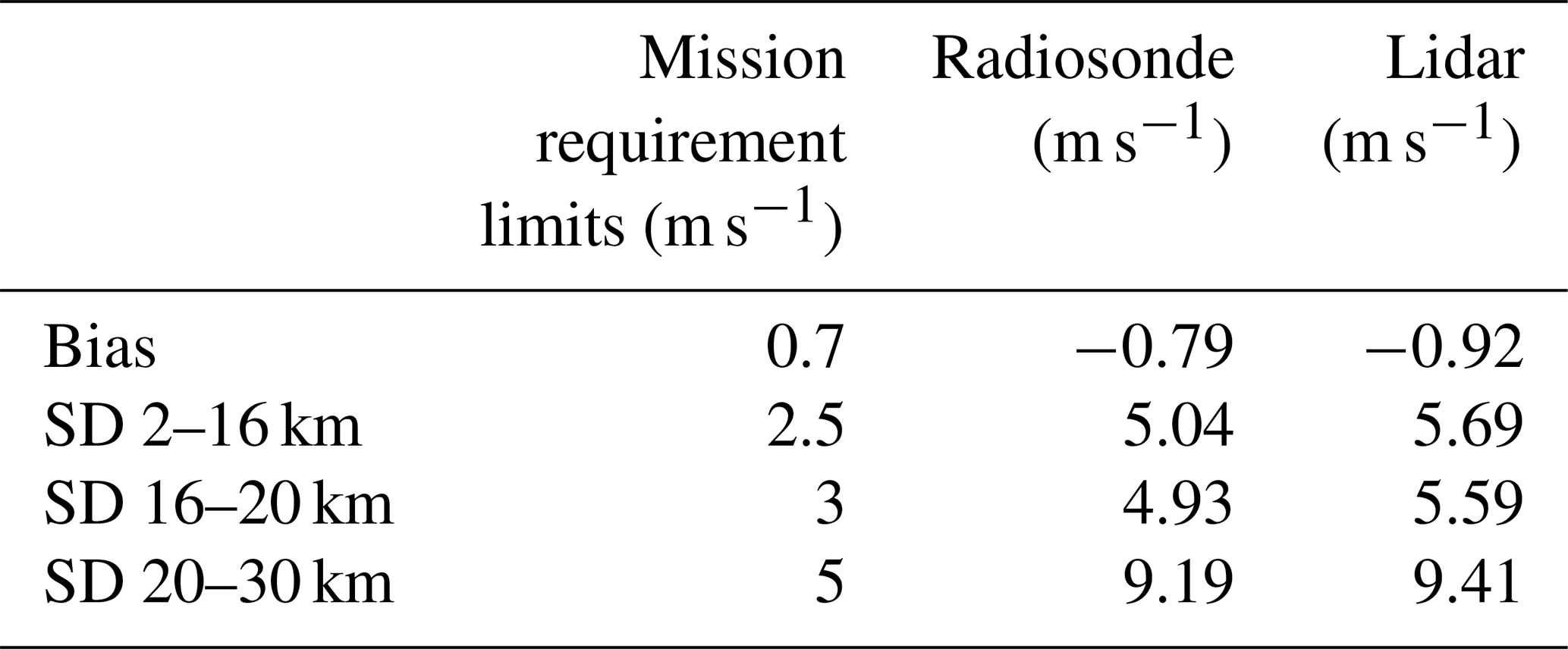
For the lidars, other cal/val campaigns report scaled MADs of 3.91 m s−1 (Wu et al. 2022), 5.21 m s−1, and 5.58 m s−1 for Iwai et al. (2021). They also report SDs of 5.98 and 4.78 m s−1 (Chen et al., 2022), 4.76 m s−1 (Wu et al., 2021), and 5.69 and 6.53 m s−1 (Iwai et al., 2021). Our results point to a scaled MAD of 6.49 m s−1 and a SD of 7.25 m s−1, further confirming other studies even if we observe bigger numbers, because of a wider altitude range comparison. It should also be noted that we do not meet the mission requirements (Ingmann and Straume, 2016), as seen in previous studies (Baars et al., 2020; Iwai et al., 2021; Martin et al., 2021; Rennie et al., 2021; Wu et al., 2022) with similar magnitudes and values. The offset between the observed SD and the mission requirement's SD does not seem to change between the free troposphere and the first kilometers of the stratosphere. The uppermost region of observation is where we reach the highest difference between the observed and the required SD – more than 4 m s−1.
Table 6Aeolus mission requirements on the bias and standard deviation (MR-100 and MR-110, Ingmann and Straume, 2016) compared to the observed bias and standard deviation, depending on the altitude level.
4.2 Case-based analysis
In this subsection, we further discuss Aeolus' capacities and performance with the help of four specific case studies. The goal is to provide an overview of the measurements by choosing representative collocations, each helping to show specificities present in the dataset. It shows that in the same conditions (i.e., spatial/temporal offsets) Aeolus can behave very differently. These measurements are part of a more extensive statistical analysis presented in the above subsection. The Fig. 5 shows the HLOS wind velocity profiles measured by the radiosonde (black), the ground-based lidar (red), and the space lidar (blue). The shadings represent the measurement error for each data point, and the radiosondes' uncertainty is between 0.4 and 1 m s−1 (Dirksen et al., 2014), which is smaller than the ground-based lidar (2.2 m s−1) (Khaykin et al., 2020) and Aeolus (4.1–4.4 m s−1) (Martin et al., 2021) uncertainties. For clarity, radiosonde wind speed uncertainties are not plotted in Fig. 5. Since Aeolus takes measurements 35∘ off-nadir, the horizontal distance of the Aeolus observations to the ground-based lidar is different for each height bin in the Aeolus wind profile. At the same time, the radiosonde drifts along the direction of local wind, making the distance between the Aeolus measurements and the radiosonde vary during the balloon sounding as a function of height. Furthermore, it is not only the distance between Aeolus and radiosonde that changes with time – the time difference between the two systems also changes with time and, therefore, also with altitude.
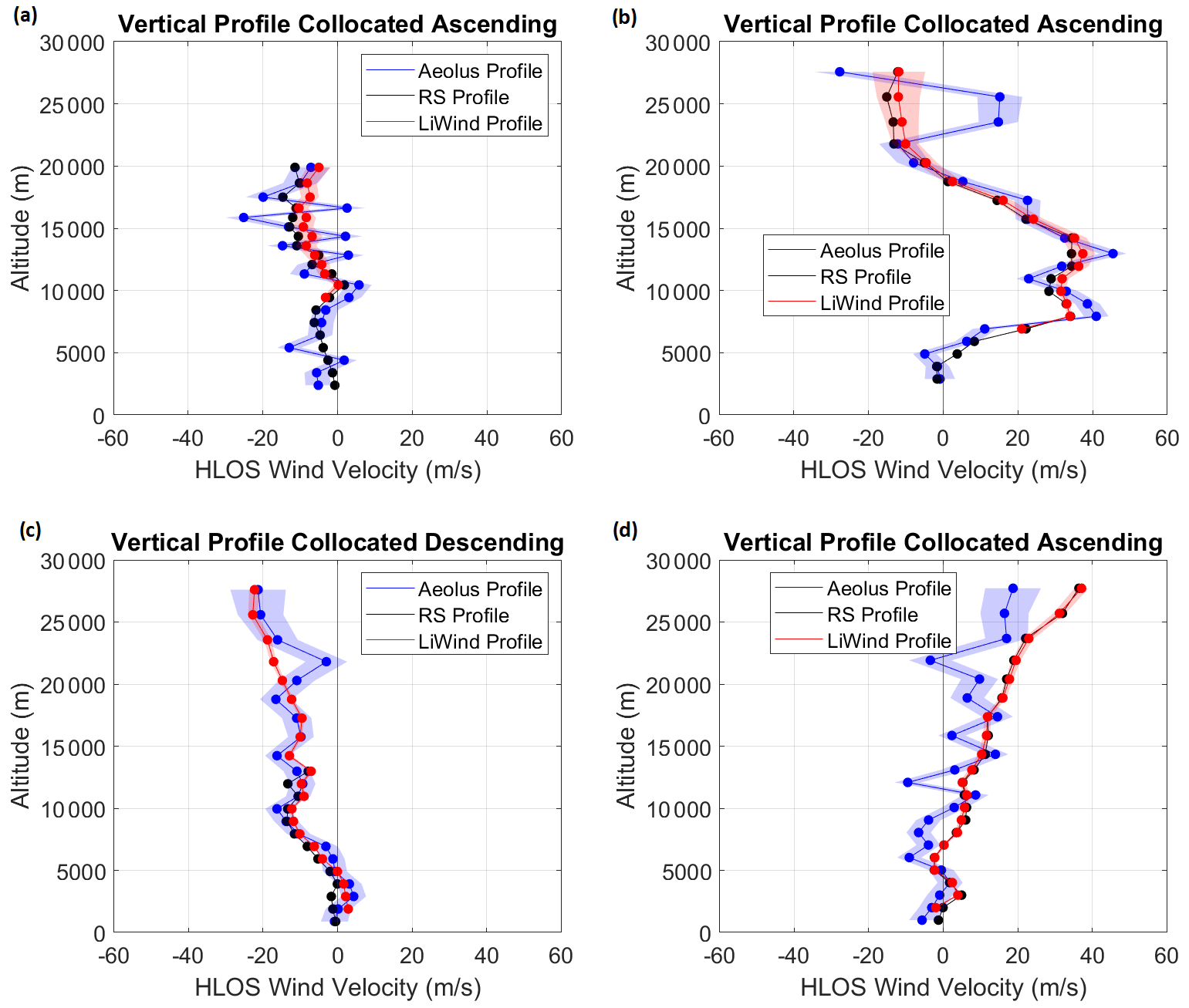
Figure 5Wind velocity profiles measured by the radiosonde (black) with the closest Aeolus Level 2B Rayleigh clear (blue) and ground-based lidar (red) profiles. The lidar and radiosonde profiles are shown with an adjusted resolution to the Aeolus range bin width. The lidar and radiosonde measurements are projected to the HLOS of Aeolus. (a) 24 February 2021 (AboVE Maido 2), (b) 9 June 2021 (AboVE Maido 2), (c) 14 December 2021 (AboVE OHP 2), and (d) 20 December 2021 (AboVE OHP 2). The shading represents the internal estimated error for each instrument.
4.2.1 Case study (a): 24 February 2021 (AboVE Maido 2) – 2B11
This collocation was taken at 14:32 UTC. Both instruments were started 30 min prior, at around 14:00 UTC. The mean measuring distance is 67 km for the radiosonde and 40 km for the lidar. The mean bias of the radiosonde is 0.46 m s−1, and the lidars' is −0.68 m s−1. The standard deviation is 6.8 and 8.8 m s−1, the scaled MAD is 6.36 and 11.38 m s−1, and correlation coefficients are 0.55 and 0.46. The figure depicts a very specific pattern of oscillating nature. Although showing a similar trend to the other two instruments (with the mean bias lower than |1| m s −1 for both reference instruments), the ALADIN shows a very particular signature between 12 and 19 km. This observation could hint toward the existence of oscillating perturbations, OPs. We could not find any literature assessing the existence of similar phenomena. Henceforth, what remains to be explained is the nature of the oscillation, which does not correspond to any known phenomenon. While the hot pixels could also play a part in this phenomenon, explaining the increase in magnitude, they cannot account for the oscillating nature (Weiler et al., 2021a).
4.2.2 Case study (b): 9 June 2021 (AboVE Maido 2) – 2B12
This collocation was taken at 14:33 UTC. Both instruments were started 30 min prior, at around 14:00 UTC. The mean spatial offset is 33 km for the radiosonde and 40.5 km for the lidar. The mean bias between Aeolus and the radiosonde is 2.52 m s−1, and the mean bias between Aeolus and the lidars is 2.22 m s−1. The standard deviations are 11.21 and 11.54 m s−1, the scaled MADs are 6.75 and 9.05 m s−1, and correlation coefficients are 0.83 and 0.84.
It is found that the Aeolus wind profile in the atmospheric boundary layer and the lower troposphere is in good agreement except for the 22 km height and higher bins of the Aeolus wind profile, which have a significant bias compared with the radiosondes and lidar-retrieved HLOS wind. These exceptionally strong deviations are observed for most AboVE-Maido-2 campaign collocations and happen specifically within the uppermost bins. The low molecular density could explain the cause of the higher values observed at high altitude levels. We conclude that, because of this mission's specific RBS, the satellite does not resolve the higher altitude ranges with enough precision since it does not receive enough backscattering.
4.2.3 Case study (c): 14 December 2021 (AboVE OHP 2) – 2B13
The third case study is from the second and most recent cal/val campaign conducted at the Observatoire de Haute-Provence. The distance to collocation is under 70 km for both instruments, and the time interval is less than 2 h. The mean bias between Aeolus and the radiosonde is 1.5 m s−1, and the mean bias between Aeolus and the lidars is 0.5 m s−1. The standard deviations are 2.84 and 4.02 m s−1, the scaled MADs are 2.85 and 3.22 m s−1, and correlation coefficients are 0.92 for radiosonde and 0.86 for lidar. The scaled MAD is exceptionally low compared to other cases, showing that ALADIN is still able to perform very well and deliver excellent results, beyond the nominal lifetime of 3 years. Here, the Rayleigh clear profile obtained by Aeolus is within a close interval to the ground-based data, except for a sudden spike appearing at around 23 km. Indeed, this spike, which is not observed on the reference lidar, could be linked to Aeolus' hot-pixel issue (Weiler et al., 2021a) since 24 hot pixels were present in the Rayleigh channel (ESA, 2021a).
4.2.4 Case study (d): 20 December 2021 (AboVE OHP 2) – 2B13
This collocation is a good example of the poor-behaving measurements Aeolus can come across because the satellite seems to miss what the lidar and the radiosonde see even within close collocation criteria (40 min difference and both instrument under 80 km). An oscillating perturbation is also present on Aeolus' profile as opposed to the reference data. Given the very close collocation, one could assume a negligibly small geophysical bias, so that the three observations would keep a general common trend. We look at an oscillating profile with significant offsets from the reference measurement. That could be interpreted as a coupling between both oscillations and hot pixels, meaning that these phenomena can co-occur. The mean bias between Aeolus and the radiosonde is −6.56 m s−1, and the mean bias between Aeolus and the lidars is −6.53 m s−1. The standard deviations are 6.84 and 7.12 m s−1, the scaled MADs are 6.42 and 6.59 m s−1, and correlation coefficients are 0.76 and 0.75.
4.3 Long-term validation
This section aims to convey an idea of the evolution of Aeolus' performance over its mission cycle, starting in September 2018. For comparisons, Météo-France sites in Réunion (21∘ S, 55∘ E) and Nîmes were used (43∘ N, 4∘ E). These sites perform twice-a-day radiosonde launches at midnight and noon, opening broader possibilities for potential collocations. Both sites have an average of 120 km of distance to collocation. The Réunion site has a time difference of 3 h on average, whereas the Nîmes site has a 5.5 h time difference.
Figure 6 shows the time series of the standard deviation of the difference between Aeolus Rayleigh clear HLOS wind and Météo-France radiosonde launches at both sites. Outlier detection was conducted on both time series using the scaled MAD technique (outliers are defined as elements more than 3 scaled MADs from the median). Also shown in Fig. 6 are the cal/val campaign observations. For this comparison, we used only Aeolus data between 5 and 22 km to exclude the uppermost bins characterized by the largest errors (Sect. 4.2).
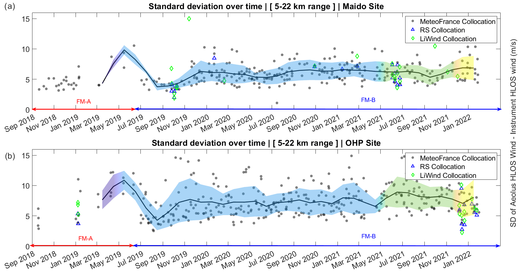
Figure 6Standard deviation of the difference between Aeolus Rayleigh clear HLOS wind and Météo-France Radiosonde HLOS wind over time (a) at the Maido observatory and (b) at the Observatoire de Haute-Provence. The Météo-France data were downsampled to Aeolus vertical resolution and projected to the HLOS of Aeolus. For radiosonde and ground-based lidar collocations, the cal/val punctual collocations are reported in the figure in blue and green markings. The black line represents the average value, and the shading represents its standard deviation. The colors are relative to the four baselines used: 2B02 (violet), 2B11 (blue), 2B12 (green), and 2B13 (yellow), in that order.
As previously mentioned, both sites have a similar average distance to the collocation; however, the time offset is larger for the Nîmes site by 2.5 h. As demonstrated in Sect. 4.1, the distance to collocation does not significantly impact the bias of the collocations. As such, this explains why both time series share a very similar trend and show the same variations specific to mission events (FM-A laser power loss, FM-B switch, etc.). We note that the standard deviation at Nîmes is higher by 1.5 m s−1 on average compared to that at Réunion. Because the distance to collocation is the same at both sites, this higher random error can be explained by the larger time offset. One can thus conclude that in terms of the collocation criteria, the temporal offset is more critical than the spatial offset when collocating satellite and ground-based wind measurements. While it might not be trivial to generalize these results to other stations with different weather and wind regimes, the findings of this study may be relevant to locations with similar characteristics.
For the Réunion time series (Fig. 6a), the October 2019 and June 2021 AboVE-Maido campaign data correspond well with the Météo-France observations, whereas the lower values could be explained by the campaign collocations with reduced geophysical bias. Additional lidar observations at Maido conducted outside the dedicated campaigns show increased random errors, supposedly due to the larger time offsets for some of these collocations (cf. Table 1). The results of the AboVE-OHP-2 campaign, displayed in Fig. 6b, show random errors similar to or lower than those inferred from the Météo-France radiosonde launches. As for the Réunion series, the lower random errors can be explained by the reduced spatial and temporal offsets for the campaign collocations.
Overall, a few conclusions can be shared across both sites of observation. Over time, we observe a slight increase in the standard deviation (+1 m s−1 on average between January 2020 and 2022). It is possible to split the time series into different periods. The early FM-B period (July 2019 to January 2020) shows the lowest random error and is consistent across both observation sites. We refer to this period as the “golden era” of Aeolus. Around mid-April 2020, the M1 bias correction introduced into the retrieval lowered the bias significantly (Weiler et al. 2021b); however, it does not appear to have an impact on the random error. From this point on, the disparity of the data stabilized, as well as their average value. The last months of the time series show a stable average value as well as its standard deviation, asserting that the satellite maintained a good precision over the last few months of 2022.
High standard deviation values could be due to hot pixels and OPs mentioned above present in the ACCDs. Previous research revealed that 6 % of the ACCD pixels are hot pixels and that around 13 % of the pixels will be affected at the end of the extended mission lifetime in spring 2023, assuming that the hot-pixel generation rate does not change (Weiler et al., 2021a). Corrections to several substantial bias sources in the Aeolus L2B winds have been implemented, including corrections to the dark current signal anomalies of single pixels (so-called hot pixels) on the accumulation charge-coupled devices (ACCDs), linear drift in the illumination of the Rayleigh/Mie spectrometers, and the telescope M1 mirror temperature variations (Reitebuch et al., 2020; Weiler et al., 2021b). Indeed, Fig. 6 confirms other studies that claim that hot pixels, laser energy, and receiving path degradation effects in ALADIN have been mitigated (Feofilov et al., 2022; Baars et al., 2020; Weiler et al., 2020). If this mitigation were not present, we would observe an increase in the standard deviation at a much higher rate (Weiler et al., 2021a). Unfortunately, due to potential calibration issues, uncorrected biases might remain in Aeolus L2B winds and may contribute to potential biases between Aeolus and the Météo-France observed winds. In addition, the Aeolus L2B winds might be biased towards the ECMWF model, as the M1 bias correction makes use of ECMWF 6 h forecasts (Rennie et al., 2021), which might also lead to suboptimal assimilation of Aeolus winds on ground comparisons (Liu et al., 2022).
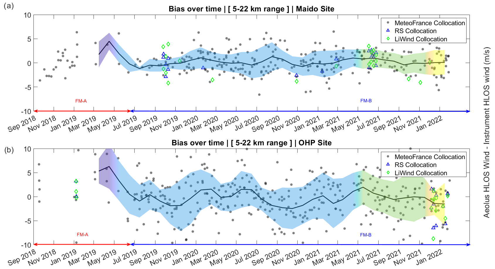
Figure 7Bias between Aeolus Rayleigh clear HLOS wind and Météo-France radiosonde HLOS wind over time (a) at the Maido observatory and (b) at the Observatoire de Haute-Provence. The Météo-France data were downsampled to Aeolus vertical resolution and projected to the HLOS of Aeolus. For radiosonde and ground-based lidar collocations, the cal/val punctual collocations are reported in the figure in blue and green markings. The black line represents the average value, and the shading represents its standard deviation. The colors are relative to the four baselines used: 2B02 (violet), 2B11 (blue), 2B12 (green), and 2B13 (yellow), in that order.
In addition to the standard deviation observed in Fig. 6, the bias can offer another opportunity to assess the evolution of the satellite's performance over time, which is shown in Fig. 7. The evolution of the bias shows a structure very similar to the previous figure, reducing its variability along the newer baselines. The expected higher variability for the OHP site is also observed, and the average value tends to be slightly lower (−1 m s−1 for OHP to 0 m s−1 for Maido) in the latest 2B13 baseline (December 2021). This figure suggests that the newer baselines help the bias converge to zero but do not have a definitive impact on the variability of the values. Additionally, the transition from reprocessed to real-time reprocessed data, which occurred on 8 October 2020 (ESA, 2021b), does not offer any apparent enhancements. Therefore, it does not support the assumption of any beneficial or detrimental changes to the data quality.
In this paper, to evaluate the accuracy and precision of the Aeolus retrieved wind results, double collocation techniques using both radiosondes and ground-based lidars were conducted. Due to the proximity of collocation and a similar functioning principle, a statistical analysis of random error, biases, and their evolution throughout the mission lifetime was performed, from the observation sites of Haute-Provence and Réunion. A total of 65 collocations were collected during periods from baseline 2B02 to 2B13.
Table 7Summary of the recent comparison campaign validation results, following Wu's (2021) referencing convention.

Similar to Wu's (2021) initiative, we summarized the recent comparison campaigns from the cal/val teams across the globe and Aeolus' lifespan. We decided to use the same statistical parameters and presentation that Wu (2021) proposed, in order to keep a consistent comparison method over several studies. Therefore, the statistical parameters include the correlation coefficient, SD, MAD, bias, slope, and intercept. We can compare our results to other instruments that were not mentioned during previous sections, such as ALADIN airborne demonstrators (A2D) (Witschas et al., 2020; Lux et al., 2020a, 2022), airborne Doppler wind lidars (DWL) (Witschas et al., 2020, 2022), and wind profiler radars (WPR) (Zuo et al., 2022; Guo et al., 2021; Belova et al., 2021; Iwai et al., 2021). Close to Wu's (2021) observations, we observe the same consistency and similarities with the more recent studies. A non-negligible proportion of the disparities between the measurements are caused by the variety of comparison ranges, ranging from the boundary layer to the mid-stratosphere.
Over time, we assess a very modest decrease in the precision of ALADIN measurements (Fig. 6) at both cal/val sites. While studies claim that the effects have been mitigated thanks to various corrections (Rennie et al., 2021; Reitebuch et al., 2020; Weiler et al., 2021b), this might not compensate for the increased error over time coming from hot pixels, the temperature of the mirror, and laser-induced contamination. Uncorrected biases might remain in Aeolus L2B winds and may contribute to potential biases between Aeolus and the Météo-France observed winds (Liu et al., 2022).
The argument made in Sect. 4.3 is that the time offset is more important than the spatial offset, in terms of impact on the collocation quality. Therefore, it should be inferred from this result that the time criterion has to be favored over the distance criterion when collocating different measurements. To do so, we showed how the distance to collocation had small effects on the bias in Sect. 4.2 and how the time difference had a significant impact on the standard deviation in Sect. 4.3. Some error sources were pointed out by previous research, e.g., hot pixels and dark current anomalies (Weiler et al., 2021a); Rayleigh wind errors introduced by angular variations (Lux et al., 2022, 2018, 2020a); vibrations introduced by the satellite platform, which affects the Q-switched master oscillator cavity length (Lux et al., 2020b); photon shot noise (Liu et al., 2006); micro-vibrations due to critical rotation speeds of the satellite's reaction wheels (Lux et al., 2021); mechanical disturbances generated by reaction wheels of the class of those embarked on Aeolus (Le, 2017); linear drift in the illumination of the Rayleigh/Mie spectrometers; and the telescope M1 mirror temperature variations (Reitebuch et al., 2020; Weiler et al., 2021b). In Sect. 4.1, we observe a steep increase in the random error above 25 km, which can be further observed in Fig. 5b. We believe that this issue, specific to the high RBS profiles, is caused by the lack of molecular backscatter. The lack of signal could result in a higher random error, but the estimated error is shown to still be within a narrow interval (±5 m s−1), compared to its observed deviation from reference measurements. Although bigger than what is shown for the previous altitude bins, the retrieved measurement error for the uppermost bins is strongly underestimated, along with the physical fact that there are fewer molecules at higher altitude levels.
In this study, we also refer to OPs, which might be a new, unreferenced, phenomenon. Over the 65 collocations, the phenomenon was observed five times. It is impossible to tell how recurrent this perturbation appears, because it requires a single profile-to-profile reference measurement, which is not something done in Aeolus to models comparisons. We note that applying a high-pass filter with the cutoff at 5 km vertical wavelength smooths out all oscillations and provides an estimation of the profile much closer to that of the reference instruments. While this is a good patch, it is not possible to apply such a filter on every wind profile, as it would probably also remove traces of physical events. One way to further improve this method would be to see how the HLOS value fluctuates from one bin to another. Since OPs tend to have a fairly constant peak-to-peak amplitude and period, it should be fairly easy to detect such patterns in the data. One way to further track down this issue would be to retrieve the L1B useful signal, as well as the SNR, to see if it could be linked to bad behavior of the optical system itself.
We observe a negative bias in most scenarios, except for the altitude range method, where the descending orbit lidar collocations show a positive bias. On average, the satellite tends to underestimate the wind speed by around 1 m s−1. Several papers cited above (Sect. 4.1 and Table 7) report similar observations.
With this study, we have addressed the performance of the ALADIN Rayleigh channel at a broad range of altitudes, from the lower troposphere to the maximum altitude of 30 km enabled by the AboVE-2 range bin setting. The performance of the ALADIN Mie channel in the lower stratosphere remains to be assessed using the lidar and radiosonde measurements at Réunion. This site was to provide the most extensive lidar observations of the 2022 Hunga Tonga volcanic eruption plumes in the stratosphere (Baron et al., 2022), which were sampled by the ALADIN Mie channels (Legras et al., 2022; Khaykin et al., 2022).
The Aeolus wind products from the first wind lidar in space, ALADIN, were validated against radiosondes and ground-based Doppler Rayleigh–Mie lidars from the observation sites of OPAR in Réunion and OHP in Haute-Provence (France). All 65 collocations were collected during periods from baseline 2B02 to 2B13, spanning January 2019 to January 2022. In summary, we find a standard deviation of 6.18 and 7.25 m s−1 and a scaled MAD of 5.37 and 6.49 m s−1 for radiosondes and lidars intercomparisons, respectively. We also find correlation coefficients of 0.82 and 0.77, slopes of 0.95 and 0.96, and y intercepts of −0.87 and −1.12 m s−1 for radiosondes and lidars intercomparisons, respectively. The biases and random errors observed are higher than those outlined in the mission requirements (Ingmann and Straume, 2016), as seen in Table 6: the bias is higher by an average of 0.15 m s−1, and the standard deviation was exceeded at every altitude level by 50 %, on average.
When collocating ground-based and satellite measurements, the time criterion was found to be more prevalent than the distance criterion in terms of choosing which one to favor, as shown in Sect. 4.3 of this study. However, it should be noted that these results may not be applicable to all stations with different weather and wind regimes and are only relevant to locations with similar characteristics. This study also showed previously undocumented phenomena (oscillating perturbations, OPs, Sect. 4.2; excessive random error in the uppermost bins above 25 km, Sect. 4.1). While the latter phenomenon can be mitigated through the use of averages between several adjacent profiles, the OP issue could be addressed by application of frequency filters, which would require further investigation.
Within this study, we have noticed range-bin and temporal wind dependencies. For the uppermost bins (above 22 km on average) enabled by the AboVE RBS, the random error is enhanced by 2–3 m s−1 for ascending and descending phases. This can be explained by the lower air density there, reducing the molecular backscatter intensity. We note that aggregation of two or more adjacent Aeolus profiles improves the comparison by 70 %. For the larger spatial offsets, the method yields poorer results compared to the altitude range method. Both methods lowered the scaled MAD on any comparison category for any instrument. Similarly to the results by Guo et al. (2021) and Zuo et al. (2022), we do not observe any significant difference between ascending and descending phases, which goes against previous observations about orbit-dependent characteristics (Rennie et al., 2021; Martin et al., 2021). Guo et al. (2021) showed slopes of 0.91 and 0.96 and intercepts of 0.47 and −1.4 m s−1, respectively. This is close to our observations. Detailing our results, the comparison of ascending phase for radiosondes collocations has a mean correlation coefficient of 0.77 and a scaled MAD of 5.58 m s−1. In contrast, the descending phase has a mean correlation coefficient of 0.91 and a scaled MAD of 4.99 m s−1. The lidar collocations in ascending phase have a mean correlation coefficient of 0.73 and a scaled MAD of 7.17 m s−1, whereas the descending phase has a mean correlation coefficient of 0.85 and a scaled MAD of 5.06 m s−1.
Overall, we recognize evolutions in the L2B data quality throughout the satellite's lifetime. Thanks to the regular measurement campaigns and the use of twice-daily Météo-France radiosondes, we managed to observe the long-term evolution of the precision of the satellite based on the standard deviation of daily collocations made between the satellite and the closest Météo-France station. As observed during the AboVE-Maido validation campaigns, the mean random error increases from 4.6 to 7.6 m s−1 between the AboVE-1 campaign (October 2019) and the AboVE-2 campaign (June 2021). For the AboVE-OHP campaigns, the mean random error increases from 5.6 to 6.4 m s−1 between the AboVE-1 campaign (January 2019) and the AboVE-2 campaign (December 2021). This is consistent with the routine observations using Météo-France's radiosondes. The early FM-B period, the golden era of Aeolus, shows the lowest random error at both sites, which has been increasing ever since.
The code used in this study can be found at https://doi.org/10.5281/zenodo.7477104 (Ratynski, 2022b).
Aeolus data are publicly available through the Aeolus online dissemination system (https://aeolus-ds.eo.esa.int/oads/access/, last access: 9 February 2022; EASA, 2022). The OHP lidar data can be obtained through the NDACC lidar database at https://ndacc.larc.nasa.gov/ (last access: 9 February 2022; NDACC, 2022). The Météo-France radiosonde data are free available at https://donneespubliques.meteofrance.fr/?fond=produit&id_produit=97&id_rubrique=33 (last access: 9 February 2022; Meteo France, 2022). The dataset used for the realization of this study can be found at https://doi.org/10.5281/zenodo.7477063 (Ratynski, 2022a).
The supplement related to this article is available online at: https://doi.org/10.5194/amt-16-997-2023-supplement.
MR and SK conceived the study. SK, RW, MR, and AH conducted the lidar measurements. AH, RW, and PK offered scientific insight. JPC and YH conducted AboVE-Maido radiosonde measurements. The paper was written by MR with contributions from all co-authors.
The contact author has declared that none of the authors has any competing interests.
Publisher’s note: Copernicus Publications remains neutral with regard to jurisdictional claims in published maps and institutional affiliations.
This article is part of the special issue “Aeolus data and their application (AMT/ACP/WCD inter-journal SI)”. It is not associated with a conference.
We gratefully thank the personnel of OPAR station (Eric Golubic, Patrick Hernandez, and Louis Mottet) and the personnel of station Gérard Mégie at OHP (Frederic Gomez, Francois Dolon, Pierre Da Conceicao, Francois Huppert, and others) for conducting the radiosonde launches and lidar operation. The work related to Aeolus validation has been performed in the frame of Aeolus Scientific Calibration and Validation Team (ACVT) activities. We thank three anonymous referees for their constructive remarks that helped improve the manuscript.
The upgrade of OHP and OPAR wind lidars was financially supported by CNES (Centre National d'Etudes Spatiales) as well as through EU FP7 ARISE and H2020 ARISE2 projects. The work by Mathieu Ratynski was carried out under a PhD fellowship co-funded by CNES and ACRI-ST. Additional funding has been provided via the CNES APR Aeolus project.
This paper was edited by Ad Stoffelen and reviewed by three anonymous referees.
Albertema, S.: Validation of Aeolus satellite wind observations with aircraft-derived wind data and the ECMWF NWP model for an enhanced understanding of atmospheric dynamics, Master thesis Utrecht Un., the Netherlands, https://dspace.library.uu.nl/handle/1874/383392 (last access: 9 February 2022), 2019.
Anderson, P. S., Ladkin, R. S., and Renfrew, I. A.: An autonomous Doppler sodar wind profiling system, J. Atmos. Ocean. Technol., 22, 1309–1325, https://doi.org/10.1175/JTECH1779.1, 2005.
Baars, H., Herzog, A., Heese, B., Ohneiser, K., Hanbuch, K., Hofer, J., Yin, Z., Engelmann, R., and Wandinger, U.: Validation of Aeolus wind products above the Atlantic Ocean, Atmos. Meas. Tech., 13, 6007–6024, https://doi.org/10.5194/amt-13-6007-2020, 2020.
Baron, A., Chazette, P., Khaykin, S., Payen, G., Marquestaut, N., Bègue, N., and Duflot, V.: Early Evolution of the Hunga-Tonga Stratospheric Aerosol Plume observed by Lidar at La Réunion (21∘ S, 55∘ E), ESS Open Archive, 6 September 2022, https://doi.org/10.1002/essoar.10512319.1, 2022.
Baumgarten, G.: Doppler Rayleigh/Mie/Raman lidar for wind and temperature measurements in the middle atmosphere up to 80 km, Atmos. Meas. Tech., 3, 1509–1518, https://doi.org/10.5194/amt-3-1509-2010, 2010.
Belova, E., Kirkwood, S., Voelger, P., Chatterjee, S., Satheesan, K., Hagelin, S., Lindskog, M., and Körnich, H.: Validation of Aeolus winds using ground-based radars in Antarctica and in northern Sweden, Atmos. Meas. Tech., 14, 5415–5428, https://doi.org/10.5194/amt-14-5415-2021, 2021.
Chanin, M. L., Garnier, A., Hauchecorne, A., and Porteneuve, J.: A Doppler lidar for measuring winds in the middle atmosphere, Geophys. Res. Lett., 16, 1273–1276, https://doi.org/10.1029/GL016i011p01273, 1989.
Chen, C., Xue, X., Sun, D., Zhao, R., Han, Y., Chen, T., Liu, H., and Zhao, Y.: Comparison of Lower Stratosphere Wind Observations From the USTC's Rayleigh Doppler Lidar and the ESA's Satellite Mission Aeolus, Earth Space Sci., 9, e2021EA002176, https://doi.org/10.1029/2021EA002176, 2022.
de Kloe, J., Stoffelen, A., Tan, D., Andersson, E., Rennie, M., Dabas, A., Poli, P., and Huber, D.: ADM-Aeolus Level-2B/2C Processor Input/Output Data Definitions Interface Control Document, available at: https://earth.esa.int/pi/esa?type=file&table=aotarget&cmd=image&alias=ADM_Aeolus_L2B_Input_Output_DD_ICD (last access: 9 August 2022), 2016.
Dirksen, R. J., Sommer, M., Immler, F. J., Hurst, D. F., Kivi, R., and Vömel, H.: Reference quality upper-air measurements: GRUAN data processing for the Vaisala RS92 radiosonde, Atmos. Meas. Tech., 7, 4463–4490, https://doi.org/10.5194/amt-7-4463-2014, 2014.
ESA: Aeolus CAL/VAL and Science Workshop, 26–29 March 2019, Frascati (Rome), Italy, https://nikal.eventsair.com/QuickEventWebsitePortal/aeolus-calval-and-science-workshop-2019/aeolus (last access: 9 August 2022), 2019.
ESA: Aeolus L1B Data Quality Report WM173, 07-15 December 2021, https://www.aeolus.esa.int/confluence/pages/viewpage.action?spaceKey=CALVAL&title=Data+Quality+Report+WM173 (last access: 9 August 2022), 2021a.
ESA: Summary of Quality of Aeolus Data Products from 2nd Reprocessing Campaign covering June 2019 to October 2020, https://earth.esa.int/eogateway/documents/20142/0/Aeolus-Summary-Reprocessing-2-DISC.pdf (last access: 23 January 2023), 2021b.
ESA: Welcome to the ESA Aeolus Online Dissemination System, aeolus, ESA [data set], https://aeolus-ds.eo.esa.int/oads/access/, last access: 9 February 2022.
Eyre, J. R., English, S. J., and Forsythe, M.: Assimilation of satellite data in numerical weather prediction. Part I: The early years, Q. J. Roy. Meteorol. Soc., 146, 49–68, https://doi.org/10.1002/qj.3654, 2020.
Feofilov, A. G., Chepfer, H., Noël, V., Guzman, R., Gindre, C., Ma, P.-L., and Chiriaco, M.: Comparison of scattering ratio profiles retrieved from ALADIN/Aeolus and CALIOP/CALIPSO observations and preliminary estimates of cloud fraction profiles, Atmos. Meas. Tech., 15, 1055–1074, https://doi.org/10.5194/amt-15-1055-2022, 2022.
Forsythe, M.: Atmospheric motion vectors: past, present and future, in: ECMWF Annual Seminar, 1–79 pp., 2007.
Guo, J., Liu, B., Gong, W., Shi, L., Zhang, Y., Ma, Y., Zhang, J., Chen, T., Bai, K., Stoffelen, A., de Leeuw, G., and Xu, X.: Technical note: First comparison of wind observations from ESA's satellite mission Aeolus and ground-based radar wind profiler network of China, Atmos. Chem. Phys., 21, 2945–2958, https://doi.org/10.5194/acp-21-2945-2021, 2021.
Hauchecorne, A. and Chanin, M.-L.: Density and temperature profiles obtained by lidar between 35 and 70 km, Geophys. Res. Lett., 7, 565–568, https://doi.org/10.1029/GL007i008p00565, 1980.
Hauchecorne, A., Chanin, M.-L., and Keckhut, P.: Climatology and trends of the middle atmospheric temperature (33–87 km) as seen by Rayleigh lidar over the south of France, J. Geophys. Res.-Atmos., 96, 15297, https://doi.org/10.1029/91JD01213, 1991.
Houchi, K., Stoffelen, A., Marseille, G. J., and De Kloe, J.: Comparison of wind and wind shear climatologies derived from high-resolution radiosondes and the ECMWF model, J. Geophys. Res.-Atmos., 115, D22123, https://doi.org/10.1029/2009JD013196, 2010.
Ingmann, P. and Straume, A. G.: ADM-Aeolus Mission Requirements Document, https://earth.esa.int/pi/esa?type=file&table=aotarget&cmd=image&alias=Aeolus_MRD (last access: 9 August 2022), 2016.
Iwai, H., Aoki, M., Oshiro, M., and Ishii, S.: Validation of Aeolus Level 2B wind products using wind profilers, ground-based Doppler wind lidars, and radiosondes in Japan, Atmos. Meas. Tech., 14, 7255–7275, https://doi.org/10.5194/amt-14-7255-2021, 2021.
Kanitz, T., Lochard, J., Marshall, J., McGoldrick, P., Lecrenier, O., Bravetti, P., Reitebuch, O., Rennie, M., Wernham, D., and Elfving, A.: Aeolus first light: first glimpse, in: International Conference on Space Optics – ICSO 2018, 659–664, https://doi.org/10.1117/12.2535982, 2019a.
Kanitz, T., Straume, A. G., Marshall, J., Lecrenier, O., Sachhieri, V., Reitebuch, O., Rennie, M., and Wernham, D.: Aeolus – 1 Year After Launch, in: IGARSS 2019 – 2019 IEEE International Geoscience and Remote Sensing Symposium, 28 July–2 August 2019, Yokohama, Japan, 4769–4770, https://doi.org/10.1109/IGARSS.2019.8898100, 2019b.
Keckhut, P., Courcoux, Y., Baray, J.-L., Porteneuve, J., Vérèmes, H., Hauchecorne, A., Dionisi, D., Posny, F., Cammas, J.-P., Payen, G., Gabarrot, F., Evan, S., Khaykin, S., Rüfenacht, R., Tschanz, B., Kämpfer, N. A., Ricaud, P., Abchiche, A., Leclair-de-Bellevue, J., and Duflot, V.: Introduction to the Maïdo Lidar Calibration Campaign dedicated to the validation of upper air meteorological parameters, JARS, 9, 094099, https://doi.org/10.1117/1.JRS.9.094099, 2015.
Khaykin S. M., Hauchecorne, A., Cammas, J.-P., Marqestaut, N., Mariscal, J.-F., Posny, F., Payen, G., Porteneuve, J., and Keckhut, P.: Exploring fine-scale variability of stratospheric wind above the tropical la reunion island using Rayleigh-Mie Doppler lidar, EPJ Web Conf. Volume 176, The 28th International Laser Radar Conference (ILRC 28), https://doi.org/10.1051/epjconf/201817603004, 2018.
Khaykin, S. M., Hauchecorne, A., Wing, R., Keckhut, P., Godin-Beekmann, S., Porteneuve, J., Mariscal, J.-F., and Schmitt, J.: Doppler lidar at Observatoire de Haute-Provence for wind profiling up to 75 km altitude: performance evaluation and observations, Atmos. Meas. Tech., 13, 1501–1516, https://doi.org/10.5194/amt-13-1501-2020, 2020.
Khaykin, S., Podglajen, A., Ploeger, F., Grooß, J.-U., Tence, F., Bekki, S., Khlopenkov, K., Bedka, K., Rieger, L., Baron, A., Godin-Beekmann, S., Legras, B., Sellitto, P., Sakai, T., Barnes, J., Uchino, O., Morino, I., Nagai, T., Wing, R., Baumgarten, G., Gerding, M., Duflot, V., Payen, G., Jumelet, J., Querel, R., Liley, B., Bourassa, A., Clouser, B., Feofilov, A., Hauchecorne, A., and Ravetta, F: Global perturbation of stratospheric water and aerosol burden by Hunga eruption, Commun. Earth Environ., 3, 316, https://doi.org/10.1038/s43247-022-00652-x, 2022.
Krisch, I. and the Aeolus DISC: Data quality of Aeolus wind measurements, EGU General Assembly 2020, Online, 4–8 May 2020, EGU2020-9471, https://doi.org/10.5194/egusphere-egu2020-9471, 2020.
Krisch, I., Preusse, P., Ungermann, J., Dörnbrack, A., Eckermann, S. D., Ern, M., Friedl-Vallon, F., Kaufmann, M., Oelhaf, H., Rapp, M., Strube, C., and Riese, M.: First tomographic observations of gravity waves by the infrared limb imager GLORIA, Atmos. Chem. Phys., 17, 14937–14953, https://doi.org/10.5194/acp-17-14937-2017, 2017.
Kumer, V.-M., Reuder, J., and Furevik, B. R.: A Comparison of LiDAR and Radiosonde Wind Measurements, Energy Proc., 53, 214–220, https://doi.org/10.1016/j.egypro.2014.07.230, 2014.
Legras, B., Duchamp, C., Sellitto, P., Podglajen, A., Carboni, E., Siddans, R., Grooß, J.-U., Khaykin, S., and Ploeger, F.: The evolution and dynamics of the Hunga Tonga–Hunga Ha'apai sulfate aerosol plume in the stratosphere, Atmos. Chem. Phys., 22, 14957–14970, https://doi.org/10.5194/acp-22-14957-2022, 2022.
Le, M. P.: Micro-disturbances in reaction wheels, PhD thesis, Technische Universiteit Eindhoven, 166 pp., https://research.tue.nl/en/publications/micro-disturbances-in-reaction-wheels (last access: 9 August 2022), 2017.
Le Pichon, A., Blanc, E., and Drob, D.: Probing high-altitude winds using infrasound, J. Geophys. Res.-Atmos., 110, D20104, https://doi.org/10.1029/2005JD006020, 2005.
Liu, H., Garrett, K., Ide, K., Hoffman, R. N., and Lukens, K. E.: A statistically optimal analysis of systematic differences between Aeolus horizontal line-of-sight winds and NOAA's Global Forecast System, Atmos. Meas. Tech., 15, 3925–3940, https://doi.org/10.5194/amt-15-3925-2022, 2022.
Liu, Z., Hunt, W., Vaughan, M., Hostetler, C., McGill, M., Powell, K., Winker, D., and Hu, Y.: Estimating random errors due to shot noise in backscatter lidar observations, Appl. Opt., 45, 4437–4447, https://doi.org/10.1364/AO.45.004437, 2006.
Lux, O., Lemmerz, C., Weiler, F., Marksteiner, U., Witschas, B., Rahm, S., Schäfler, A., and Reitebuch, O.: Airborne wind lidar observations over the North Atlantic in 2016 for the pre-launch validation of the satellite mission Aeolus, Atmos. Meas. Tech., 11, 3297–3322, https://doi.org/10.5194/amt-11-3297-2018, 2018.
Lux, O., Lemmerz, C., Weiler, F., Marksteiner, U., Witschas, B., Rahm, S., Geiß, A., and Reitebuch, O.: Intercomparison of wind observations from the European Space Agency's Aeolus satellite mission and the ALADIN Airborne Demonstrator, Atmos. Meas. Tech., 13, 2075–2097, https://doi.org/10.5194/amt-13-2075-2020, 2020a.
Lux, O., Wernham, D., Bravetti, P., McGoldrick, P., Lecrenier, O., Riede, W., D'Ottavi, A., Sanctis, V. de, Schillinger, M., Lochard, J., Marshall, J., Lemmerz, C., Weiler, F., Mondin, L., Ciapponi, A., Kanitz, T., Elfving, A., Parrinello, T., and Reitebuch, O.: High-power and frequency-stable ultraviolet laser performance in space for the wind lidar on Aeolus, Opt. Lett., 45, 1443–1446, https://doi.org/10.1364/OL.387728, 2020b.
Lux, O., Lemmerz, C., Weiler, F., Kanitz, T., Wernham, D., Rodrigues, G., Hyslop, A., Lecrenier, O., McGoldrick, P., Fabre, F., Bravetti, P., Parrinello, T., and Reitebuch, O.: ALADIN laser frequency stability and its impact on the Aeolus wind error, Atmos. Meas. Tech., 14, 6305–6333, https://doi.org/10.5194/amt-14-6305-2021, 2021.
Lux, O., Lemmerz, C., Weiler, F., Marksteiner, U., Witschas, B., Rahm, S., Geiß, A., Schäfler, A., and Reitebuch, O.: Retrieval improvements for the ALADIN Airborne Demonstrator in support of the Aeolus wind product validation, Atmos. Meas. Tech., 15, 1303–1331, https://doi.org/10.5194/amt-15-1303-2022, 2022.
Martin, A., Weissmann, M., Reitebuch, O., Rennie, M., Geiß, A., and Cress, A.: Validation of Aeolus winds using radiosonde observations and numerical weather prediction model equivalents, Atmos. Meas. Tech., 14, 2167–2183, https://doi.org/10.5194/amt-14-2167-2021, 2021.
Meteo France: Données publiques, Observations d'altitude (Radio sondages), Meteo France [data set], https://donneespubliques.meteofrance.fr/?fond=produit&id_produit=97&id_rubrique=33, last access: 9 February 2022.
NDACC: Measurement Stations, NDACC [data set], https://ndacc.larc.nasa.gov/, last access: 9 February 2022.
Prudden, S., Fisher, A., Marino, M., Mohamed, A., Watkins, S., and Wild, G.: Measuring wind with Small Unmanned Aircraft Systems, J. Wind Eng. Ind. Aerodyn., 176, 197–210, https://doi.org/10.1016/j.jweia.2018.03.029, 2018.
Ratynski, M.: Dataset used for the study of “Validation of Aeolus wind profiles using ground-based lidar and radiosonde observations at La Réunion Island and the Observatoire de Haute Provence”, Zenodo [data set], https://doi.org/10.5281/zenodo.7477063, 2022a.
Ratynski, M.: Programs used for the study of “Validation of Aeolus wind profiles using ground-based lidar and radiosonde observations at La Réunion Island and the Observatoire de Haute Provence”, Zenodo [code], https://doi.org/10.5281/zenodo.7477104, 2022b.
Reitebuch, O.: Wind Lidar for Atmospheric Research, in: Atmospheric Physics: Background – Methods – Trends, edited by: Schumann, U., Springer, Berlin, Heidelberg, 487–507, https://doi.org/10.1007/978-3-642-30183-4_30, 2012.
Reitebuch, O., Huber, D., and Nikolaus, I.: Algorithm Theoretical Basis Document ATBD: ADM-Aeolus Level 1B Products, https://earth.esa.int/pi/esa?type=file&table=aotarget&cmd=image&alias=ADM_Aeolus_L1B_Algorithm_TBD (last access: 9 August 2022), 2014.
Reitebuch, O., Lemmerz, C., Lux, O., Marksteiner, U., Rahm, S., Weiler, F., Witschas, B., Meringer, M., Schmidt, K., Huber, D., Nikolaus, I., Geiß, A., Vaughan, M., Dabas, A., Flament, T., Stieglitz, H., Isaksen, L., Rennie, M., de Kloe, J., Marseille, G.-J., Stoffelen, A., Wernham, D., Kanitz, T., Straume, A.-G., Fehr, T., von Bismark, J., Floberghagen, R., and Parrinello, T.: Initial assessment of the performance of the first Wind Lidar in space on Aeolus, EPJ Web Conf., 237, 01010, https://doi.org/10.1051/epjconf/202023701010, 2020.
Rennie, M. P. and Isaksen, L.: The NWP impact of Aeolus level-2B winds at ECMWF, ECMWF Technical Memorandum 864, https://doi.org/10.21957/alift7mhr, 2020.
Rennie, M. P., Isaksen, L., Weiler, F., de Kloe, J., Kanitz, T., and Reitebuch, O.: The impact of Aeolus wind retrievals on ECMWF global weather forecasts, Q. J. Roy. Meteorol. Soc., 147, 3555–3586, https://doi.org/10.1002/qj.4142, 2021.
Rennie, M. P., Tan, D., Andersson, E., Poli, P., Dabas, A., De Kloe, J., Marseille, G.-J., and Stoffelen, A.: Aeolus Level-2B Algorithm Theoretical Basis Document, ECMWF, https://confluence.ecmwf.int/display/AEOL/L2B+pro (last access: 9 February 2022), 2020.
Rogers, R. R., Ecklund, W. L., Carter, D. A., Gage, K. S., and Ethier, S. A.: Research Applications of a Boundary-Layer Wind Profiler, B. Am. Meteorol. Soc., 74, 567–580, https://doi.org/10.1175/1520-0477(1993)074<0567:RAOABL>2.0.CO;2, 1993.
Rüfenacht, R., Kämpfer, N., and Murk, A.: First middle-atmospheric zonal wind profile measurements with a new ground-based microwave Doppler-spectro-radiometer, Atmos. Meas. Tech., 5, 2647–2659, https://doi.org/10.5194/amt-5-2647-2012, 2012.
Ruppert, D.: Statistics and Data Analysis for Financial Engineering, 1st edn., Springer Texts in Statistics, Springer, New York, NY, USA, https://doi.org/10.1007/978-1-4419-7787-8, 2011.
Schillinger, M., Morancais, D., Fabre, F., and Culoma, A. J. F.: ALADIN: the lidar instrument for the AEOLUS mission, in: Sensors, Systems, and Next-Generation Satellites VI, 40–51, https://doi.org/10.1117/12.463024, 2003.
She, C. Y., Li, T., Williams, B. P., Yuan, T., and Picard, R. H.: Concurrent OH imager and sodium temperature/wind lidar observation of a mesopause region undular bore event over Fort Collins/Platteville, Colorado, J. Geophys. Res.-Atmos., 109, D22107, https://doi.org/10.1029/2004JD004742, 2004.
Souprayen, C., Garnier, A., Hertzog, A., Hauchecorne, A., and Porteneuve, J.: Doppler wind lidar for atmospheric measurements. I. Instrumental setup, validation, and first climatological results, Appl Opt., 20, 2410–2421, https://doi.org/10.1364/ao.38.002410, 1999.
Stoffelen, A., Pailleux, J., Källén, E., Vaughan, J. M., Isaksen, L., Flamant, P., Wergen, W., Andersson, E., Schyberg, H., Culoma, A., Meynart, R., Endemann, M., and Ingmann, P.: The Atmospheric Dynamics Mission for Global Wind Field Measurement, B. Am. Meteorol. Soc., 86, 73–88, https://doi.org/10.1175/BAMS-86-1-73, 2005.
Stoffelen, A., Benedetti, A., Borde, R., Dabas, A., Flamant, P., Forsythe, M., Hardesty, M., Isaksen, L., Källén, E., Körnich, H., Lee, T., Reitebuch, O., Rennie, M., Riishøjgaard, L.-P., Schyberg, H., Straume, A. G., and Vaughan, M.: Wind Profile Satellite Observation Requirements and Capabilities, B. Am. Meteorol. Soc., 101, E2005–E2021, https://doi.org/10.1175/BAMS-D-18-0202.1, 2020.
Straume, A. G., Rennie, M., Isaksen, L., de Kloe, J., Marseille, G.-J., Stoffelen, A., Flament, T., Stieglitz, H., Dabas, A., Huber, D., Reitebuch, O., Lemmerz, C., Lux, O., Marksteiner, U., Weiler, F., Witschas, B., Meringer, M., Schmidt, K., Nikolaus, I., Geiß, A., Flamant, P., Kanitz, T., Wernham, D., von Bismarck, J., Bley, S., Fehr, T., Floberghagen, R., and Parrinello, T.: ESA's space-based Doppler-Rayleighwind lidar mission Aeolus – First wind and aerosol product assessment results, EPJ Web Conf., 237, 01007, https://doi.org/10.1051/epjconf/202023701007, 2020.
Sun, B., Reale, A., Seidel, D. J., and Hunt, D. C.: Comparing radiosonde and COSMIC atmospheric profile data to quantify differences among radiosonde types and the effects of imperfect collocation on comparison statistics, J. Geophys. Res.-Atmos., 115, D23104, https://doi.org/10.1029/2010JD014457, 2010.
Sun, X. J., Zhang, R. W., Marseille, G. J., Stoffelen, A., Donovan, D., Liu, L., and Zhao, J.: The performance of Aeolus in heterogeneous atmospheric conditions using high-resolution radiosonde data, Atmos. Meas. Tech., 7, 2695–2717, https://doi.org/10.5194/amt-7-2695-2014, 2014.
Tan, D. G. H., Rennie, M., Andersson, E., Poli, P., Dabas, A., de Kloe, J., Marseille, G.-J., and Stoffelen, A.: Aeolus Level-2B Algorithm Theoretical Basis Document, Tech. Rep., AE-TN-ECMWFL2BP-0023, v. 3.0, 109 pp., https://earth.esa.int/eogateway/missions/aeolus/data (last access: 9 August 2022), 2017.
Weiler, F., Kanitz, T., Wernham, D., Rennie, M., Huber, D., Schillinger, M., Saint-Pe, O., Bell, R., Parrinello, T., and Reitebuch, O.: Characterization of dark current signal measurements of the ACCDs used on board the Aeolus satellite, Atmos. Meas. Tech., 14, 5153–5177, https://doi.org/10.5194/amt-14-5153-2021, 2021a.
Weiler, F., Rennie, M., Kanitz, T., Isaksen, L., Checa, E., de Kloe, J., Okunde, N., and Reitebuch, O.: Correction of wind bias for the lidar on board Aeolus using telescope temperatures, Atmos. Meas. Tech., 14, 7167–7185, https://doi.org/10.5194/amt-14-7167-2021, 2021b.
Witschas, B., Lemmerz, C., Geiß, A., Lux, O., Marksteiner, U., Rahm, S., Reitebuch, O., and Weiler, F.: First validation of Aeolus wind observations by airborne Doppler wind lidar measurements, Atmos. Meas. Tech., 13, 2381–2396, https://doi.org/10.5194/amt-13-2381-2020, 2020.
Witschas, B., Lemmerz, C., Geiß, A., Lux, O., Marksteiner, U., Rahm, S., Reitebuch, O., Schäfler, A., and Weiler, F.: Validation of the Aeolus L2B wind product with airborne wind lidar measurements in the polar North Atlantic region and in the tropics, Atmos. Meas. Tech., 15, 7049–7070, https://doi.org/10.5194/amt-15-7049-2022, 2022.
Wu, S., Sun, K., Dai, G., Wang, X., Liu, X., Liu, B., Song, X., Reitebuch, O., Li, R., Yin, J., and Wang, X.: Inter-comparison of wind measurements in the atmospheric boundary layer and the lower troposphere with Aeolus and a ground-based coherent Doppler lidar network over China, Atmos. Meas. Tech., 15, 131–148, https://doi.org/10.5194/amt-15-131-2022, 2022.
Xia, H., Dou, X., Sun, D., Shu, Z., Xue, X., Han, Y., Hu, D., Han, Y., and Cheng, T.: Mid-altitude wind measurements with mobile Rayleigh Doppler lidar incorporating system-level optical frequency control method, Opt. Express, 20, 15286–15300, https://doi.org/10.1364/OE.20.015286, 2012.
Yan, W. Y., Shaker, A., and El-Ashmawy, N.: Urban land cover classification using airborne LiDAR data: A review, Remote Sens. Environ., 158, 295–310, https://doi.org/10.1016/j.rse.2014.11.001, 2015.