The GeoCarb greenhouse gas retrieval algorithm: simulations and sensitivity to sources of uncertainty

The Geostationary Carbon Cycle Observatory (GeoCarb) was selected as NASA's second Earth Venture Mission (EVM-2). The scientific objectives of GeoCarb were to advance our knowledge of the carbon cycle, in particular, land–atmosphere fluxes of the greenhouse gases carbon dioxide (CO₂) and methane (CH₄) and the effects of these fluxes on the Earth's radiation budget. GeoCarb would retrieve column-integrated dry-air mole fractions of CO₂ ($X_{{\mathrm{CO}}_{\mathrm{2}}}$), CH₄ ($X_{{\mathrm{CH}}_{\mathrm{4}}}$) and CO (X_CO), important for understanding tropospheric chemistry), in addition to solar-induced fluorescence (SIF), from hyperspectral resolution measurements in the O₂ A-band at 0.76 µm, the weak CO₂ band at 1.6 µm, the strong CO₂ band at 2.06 µm, and a CH₄/CO band at 2.32 µm. Unlike its predecessors (OCO-2/3, GOSAT-1/2, TROPOMI), GeoCarb would be in a geostationary orbit with a sub-satellite point centered over the Americas. This orbital configuration combined with its high-spatial-resolution imaging capabilities would provide an unprecedented view of these quantities on spatial and temporal scales accurate enough to resolve sources and sinks to improve land–atmosphere CO₂ and CH₄ flux calculations and reduce the uncertainty of these fluxes.

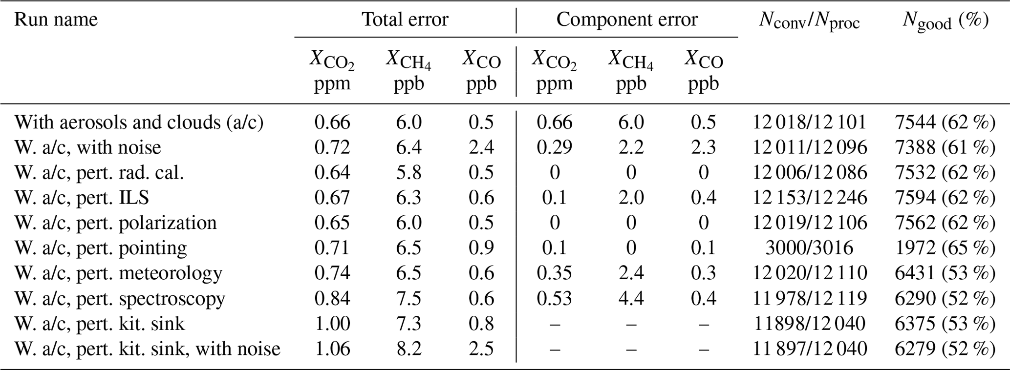
This paper will present a description of the GeoCarb instrument and the L2 retrieval algorithms which will be followed by simulation experiments to determine an error budget for each target gas. Several sources of uncertainty will be explored, including that from the instrument calibration parameters for radiometric gain, the instrument line shape (ILS), the polarization, and the geolocation pointing, in addition to forward model parameters including meteorology and spectroscopy, although there are some other instrument-related sources of uncertainty that are left out for this study, including that from “smile”, the keystone effect, stray light, detector persistence, and scene inhomogeneity. The results indicate that the errors (1σ) are less than the instrument's multi-sounding precision requirements of 1.2 ppm, 10 ppb, and 12 ppb (10 %), for $X_{{\mathrm{CO}}_{\mathrm{2}}}$, $X_{{\mathrm{CH}}_{\mathrm{4}}}$, and X_CO, respectively. In particular, when considering the sources of uncertainty separately and in combination (all sources included), we find overall RMSEs of 1.06 ppm for $X_{{\mathrm{CO}}_{\mathrm{2}}}$, 8.2 ppb for $X_{{\mathrm{CH}}_{\mathrm{4}}}$, and 2.5 ppb for X_CO, respectively. Additionally, we find that, as expected, errors in $X_{{\mathrm{CO}}_{\mathrm{2}}}$ and $X_{{\mathrm{CH}}_{\mathrm{4}}}$ are dominated by forward model and other systematic errors, while errors in X_CO are dominated by measurement noise.

It is important to note that the GeoCarb mission was canceled by NASA; however, the instrument is still in development and will be delivered to NASA, in full, with the hope that it will eventually be adopted in a future mission proposal.

1 Introduction

Carbon dioxide (CO₂) is the dominant anthropologically produced greenhouse gas (GHG) in the atmosphere. Its rapid increase in the last 170 years, due primarily to the use of fossil fuels, is changing the Earth's radiation budget leading to an increase in the mean temperature of the Earth's surface and resulting in secondary changes to the Earth's climate, including changes in weather and surface processes (Intergovernmental Panel on Climate Change (IPCC), 2021). Methane (CH₄) is the second most important anthropologically produced GHG with several sources, including oil and gas mining, agriculture, coal mines, and municipal waste. Finally, measuring carbon monoxide (CO) in the atmosphere is important for our understanding of tropospheric chemistry as a precursor to ozone (O₃), which is a pollutant in the troposphere (Granier et al., 1999; Bergamaschi et al., 2000), and is the primary sink for the hydroxyl radical (OH) (Crutzen, 1973; Logan et al., 1981), the concentration of which is important in estimating the oxidizing capacity of the atmosphere and ultimately the ability of the atmosphere to remove CH₄. Anthropogenic sources of CO include fossil fuel combustion and biomass burning (Kanakidou and Crutzen, 1999).

It is vital to make measurements of the these gases, on spatial and temporal resolutions accurate enough to resolve sources and sinks, whether natural or anthropogenic (Rayner and O'Brien, 2001; Shindell et al., 2006; Miller et al., 2007; Baker et al., 2010). These measurements are then used in GHG flux inversion models (Bergamaschi et al., 2009; Crowell et al., 2018; Nassar et al., 2017; Sellers et al., 2018) to improve our understanding of GHG fluxes between the atmosphere and surface and, ultimately, in Earth system models to understand the many complex climate feedbacks that lead to climate change (Sellers et al., 2018). Accurate measurements can be made from ground-based networks (Wunch et al., 2011a, 2017), but these surface-based measurements lack sufficient global coverage to estimate sources and sinks for all regions of the globe, especially in the poorly sampled tropics (Gurney et al., 2003). Measurements of GHG concentrations from space have been shown to help fill this gap and provide measurements on spatial scales that can resolve sources and sinks, therefore reducing uncertainty in climate model predictions (Hakkarainen et al., 2016; Jacob et al., 2016; Buchwitz et al., 2017).

In the last few decades, many satellite-based missions dedicated to measuring greenhouse gas concentrations have been successfully implemented, almost all of which are still currently acquiring data, and there are several that are planned for the future. The common objective of these missions is to measure the column-integrated dry-air mole fractions of CO₂, CH₄, and/or CO identified as $X_{{\mathrm{CO}}_{\mathrm{2}}}$, $X_{{\mathrm{CH}}_{\mathrm{4}}}$, and X_CO, respectively, with the goal of resolving sources and sinks of these gases. The Atmospheric Infrared Sounder (AIRS) is one of the first sensors that demonstrated the ability to measure CO₂ concentration (Chevallier et al., 2005), and the Measurement of Pollution in the Troposphere (MOPITT) instrument was the first instrument to demonstrate the ability to measure CO (Deeter et al., 2003; Edwards et al., 2004) in the atmosphere in the NIR.

It turns out that there is more signal to make measurements to estimate greenhouse gas surface fluxes in the near-infrared (NIR) when observed at a high spectral resolution in the so-called “weak” CO₂ band at 1.61 µm and the “strong” CO₂ band at 2.1 µm. Combined with the 0.76 µm O₂ A-band, the three bands provide sensitivity to other atmospheric characteristics, including surface pressure, temperature, aerosols and clouds, and the surface, that must be resolved to retrieve X_gas at the accuracy required to constrain sources and sinks. There have been many successfully implemented polar orbiting missions, led by countries across the world, that are partially or completely dedicated to measuring greenhouse gases by using hyperspectral measurements in these bands. These include SCIAMACHY (Bovensmann et al., 1999); TROPOMI (Veefkind et al., 2012); GOSAT (Kuze et al., 2009) and GOSAT-2 (Suto et al., 2021), using a Fourier transform spectrometer; OCO-2 (Crisp et al., 2004) and OCO-3 (Eldering et al., 2019), with very similar measurement spectra compared to the GOSAT's but using a grating spectrometer; and, finally, TanSat (Yang et al., 2018), which is similar in design to the OCOs. Future missions include the third of the GOSAT series GOSAT-GW (Matsunaga and Tanimoto, 2022), Microcarb (Pascal et al., 2017), Sentinel-5/UVNS (Irizar et al., 2019), TanSat-2 (Wu et al., 2023), and the very ambitious constellation pair of satellites for CO2M (Sierk et al., 2021). All of these missions vary in spatial coverage, spatial resolution, and spectral resolution. The one attribute that they have in common is that they are all on polar orbiting platforms, which unfortunately limits their temporal resolution.

In addition, the 0.76 µm O₂ A-band measurements made by these instruments include Fraunhofer lines from which solar-induced fluorescence (SIF) can be retrieved (Joiner et al., 2012; Frankenberg et al., 2014; Somkuti et al., 2021) which is proportional to the photosynthetic activity of vegetation while considering several other factors including vegetation type and temporal variations. Subsequently, the rate of photosynthesis affects the rate of the uptake of CO₂. These measurements of SIF can then be used to improve carbon flux inversion model results.

The planned Geostationary Carbon Cycle Observatory (GeoCarb) differs from the polar orbiting missions in that it is in a geostationary orbit centered over the American continents (Moore III et al., 2018). This approach has also been proposed before (Xi et al., 2015). In a geostationary configuration, GeoCarb will have the temporal resolution to resolve carbon cycle characteristics that can be more difficult with polar orbiters. The mission concept has been investigated including an initial investigation of the projected performance (Polonsky et al., 2014); a study of polarization dependence (O'Brien et al., 2015); and, finally, an investigation of the ability of a geostationary mission like GeoCarb to resolve greenhouse gas emissions on a shorter temporal scale (O'Brien et al., 2016; Rayner et al., 2002).

Of course, radiometric measurements need to be converted to measurements of the physical quantities of interest using a retrieval algorithm, which is essentially the inversion of a forward model. In this case, column-integrated dry-air mole fractions (X_gas) are the L2 products of use to the wider scientific community. In almost all the missions described above, a form of an optimal estimation (OE)-based algorithm for use in atmospheric retrievals is used, the application of which was formally presented by Rodgers (2004), although some of these inversions employ alternative approaches. Most of these methods are identified as so-called full-physics approaches in which the forward model approximates the physics as closely as practicably possible. The methods for these problems include linear methods such as the Weighting Function Modified Differential Optical Absorption Spectroscopy approach (WFM_DOAS) (Buchwitz et al., 2000) or nonlinear methods based on Newtonian iteration with some form of numerical regularization (Doicu et al., 2010). WFM_DOAS has been shown to be viable for SCIAMACHY, TROPOMI, GOSAT, and OCO-2 measurements for all three gases of interest (Buchwitz et al., 2005, 2006, 2017) and in a modified form with Full Spectral Initiation (FSI) to deal with pressure and temperature dependence of absorption lines (Frankenberg et al., 2005; Barkley et al., 2006). Other algorithms have been presented to deal with the photon path length extension by aerosols (Bril et al., 2007; Butz et al., 2009) and to deal with the computational burdens of accounting for these aerosols (Reuter et al., 2017). Nonlinear approaches, although more computationally intensive, are being used for the same selection of instruments (Buchwitz et al., 2017) in order to obtain as much information as possible in what is a largely an unconstrained optimal inversion. This is especially true in the case of resolving aerosol/cloud properties (Reuter et al., 2010). There are several OE algorithms for the retrieval of $X_{{\mathrm{CO}}_{\mathrm{2}}}$, $X_{{\mathrm{CH}}_{\mathrm{4}}}$, and/or X_CO applied to measurements from instruments including AIRS (Chevallier et al., 2005), with measurements in the IR or in the NIR: SCIAMACHY (Butz et al., 2010), TROPOMI (Hu et al., 2016; Landgraf et al., 2016), GOSAT-1/2 (Yokota et al., 2009; Yoshida et al., 2011), and OCO-2/3 (Connor et al., 2008; O'Dell et al., 2012; Crisp et al., 2012; O'Dell et al., 2018). In some cases, due to the convenient generality of OE, the algorithms can be applied to a number of instruments, including the use of the Atmospheric Concentrations from Space (ACOS) algorithm (O'Dell et al., 2012; Crisp et al., 2012) and the RemoTeC algorithm (Butz et al., 2009, 2010). As first proposed in Polonsky et al. (2014), for GeoCarb we use the heritage from the ACOS retrieval algorithm, currently used for OCO-2, OCO-3, and GOSAT L2 products, to simultaneously retrieve $X_{{\mathrm{CO}}_{\mathrm{2}}}$, $X_{{\mathrm{CH}}_{\mathrm{4}}}$, and/or X_CO from GeoCarb measurements.

In this paper we formally present the GeoCarb L2 OE algorithm and build on previous research with simulation experiments to determine an error budget for each target gas. SIF measurements from GeoCarb have been previously discussed in Somkuti et al. (2021) and are not further discussed here unless otherwise noted. In Sect. 2 the GeoCarb mission is discussed including its orbital configuration, the instrument characteristics, and the current challenges faced. Section 3 discusses the details of the GeoCarb L2 retrieval algorithm including the inversion methodology, forward model, state vector, and both pre- and post-processing. Section 4 describes the analysis setup including the scan strategy used, the details of the measurement data simulations, and the details of the individual perturbation experiments. In Sect. 5 the results of the perturbation experiments are presented, along with an error budget table derived from the results. Finally, in Sect. 6, some concluding remarks are given, including some points to take away from the research and an outlook of future work.

It is important to note that this study has similarities with Polonsky et al. (2014) and O'Brien et al. (2015), hereafter referred to as P2014 and O2015, respectively. These similarities include that the same four bands are used. The same three gases are retrieved (CO₂, CH₄, and CO). The simulation of synthetic radiances is performed with effectively the same code base. Finally, our meteorology and polarization tests are similar to those performed in P2014 and O2015, respectively.

Differences with P2014 and O2015 include that there are theoretical instrument model updates that reflect the current design vs. that used in P2014 and O2015, including the radiometric calibration, instrument line shape, and polarization. Our L2FP algorithm builds off of a more recent version of the ACOS L2FP algorithm. The previous publications simulate whole global, polar orbits. We use a real geostationary observation strategy similar to that envisioned for GeoCarb. The previous publications discuss “descope” options in terms of using less bands. We do not, as these were no longer considered at the time. We retrieved profiles of CH₄ and CO concentrations rather than profile scaling factors and calculated averaging kernels (AKs) for these gases from those profile retrievals. P2014 and O2015 did not test sensitivities to any instrument errors. We test sensitivities to radiometric calibration, instrument line shape, polarization, and pointing. However, as noted later, there are other instrument errors that are left for future studies. Finally, we include sensitivity to spectroscopic errors such as that explored by Connor et al. (2016) for OCO-2 in the context of $X_{{\mathrm{CO}}_{\mathrm{2}}}$ retrievals.

Finally, it is also important to note that the GeoCarb mission was canceled by NASA; however, the instrument is still in development and will be delivered to NASA, in full, with the hope that it will eventually be adopted in a future mission proposal.

2 GeoCarb mission and instrument

GeoCarb (Moore III et al., 2018) was selected as the NASA's second Earth Venture Mission (EVM-2). The scientific objectives of GeoCarb are to advance our knowledge of the carbon cycle, in particular land–atmosphere fluxes of carbon dioxide (CO₂) and methane (CH₄). This requires measurements of column-integrated dry-air mole fractions of CO₂, CH₄, and CO, in addition to SIF, at urban to continental scales and at spatial and temporal resolutions that are sufficient enough to significantly improve land–atmosphere CO₂ and CH₄ flux estimates and reduce the uncertainty of these fluxes.

To meet its scientific objectives, the GeoCarb mission is developing a multi-band, hyperspectral, Littrow grating mapping spectrometer (GMS) which will be hosted on a satellite in a geostationary orbit with a sub-satellite point (SSP) that is currently set to be 103^∘ west longitude, although the SSP may change when the host platform is finalized. GeoCarb will measure reflected sunlight in four absorption bands and retrieve column-integrated dry-air mole fractions of CO₂, CH₄, and CO known as $X_{{\mathrm{CO}}_{\mathrm{2}}}$, $X_{{\mathrm{CH}}_{\mathrm{4}}}$, and X_CO, respectively, defined by

$$\begin{array}{}\text{(1)}& X_{\mathrm{gas}}={\displaystyle \frac{{\int }_{\mathrm{0}}^{\mathrm{\infty }}{u}_{\mathrm{gas}}\left(z\right)N_{\mathrm{d}}\left(z\right)\mathrm{d}z}{{\int }_{\mathrm{0}}^{\mathrm{\infty }}{N}_{\mathrm{d}}\left(z\right)\mathrm{d}z}},\end{array}$$

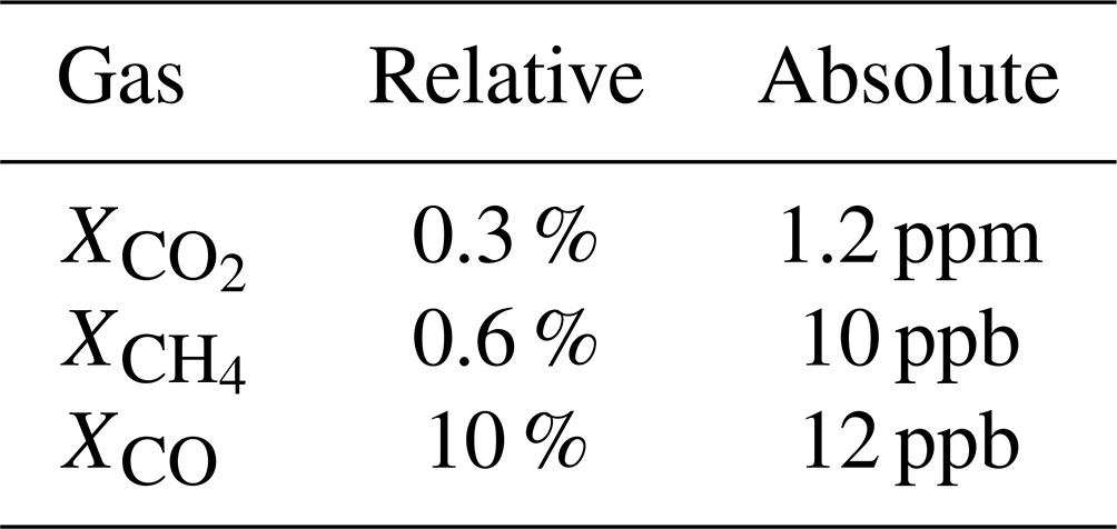
where u_gas(z) is the gas mole fraction with respect to dry air at altitude z, and N_d(z) is the total molecular number density of dry air at altitude z. The relative and absolute mission precision requirements for X_gas are listed in Table 1. These requirements are specifically for a multi-sounding precision of at least 100 aerosol- and cloud-free soundings (vertically integrated AOT + COT < 0.3, where AOT is aerosol optical thickness, and COT is cloud optical thickness), as determined against colocated Total Carbon Column Observing Network (TCCON) observations (Wunch et al., 2017).

Table 1 GeoCarb multi-sounding precision requirements for the primary target trace gases.

The four GeoCarb bands, listed in Table 2 and plotted in Fig. 1, include the O₂ A-band at 0.765 µm, the weak CO₂ band at 1.606 µm, the strong CO₂ band at 2.065 µm, and a CH₄/CO band at 2.323 µm (referred to as the CH₄ band hereafter). The four bands have spectral resolutions Δλ, defined as the full width at half maximum (FWHM) of the instrument line shape (ILS), of 0.044, 0.091, 0.114, and 0.129 nm, with resolving powers ($\mathit{\lambda }/\mathit{\delta }\mathit{\lambda }$) of roughly 17 400, 17 600, 18 100, and 18 000, respectively. The required signal-to-noise ratios are listed in Table 2 for each band along with the relative reference radiance levels. The O₂ A-band provides information on surface pressure, clouds, and aerosols. In addition, the O₂ A-band includes Fraunhofer lines from which SIF can be retrieved. The weak CO₂ band and the strong CO₂ band provide information on column CO₂ fractions and clouds and aerosols, while the strong CO₂ band also provides information on H₂O concentration. These first three bands are similar in spectral range and resolution to those on OCO-2 and OCO-3. The fourth band adds the ability to retrieve CH₄ and CO and also provides information on H₂O and hydrogen–deuterium oxide (HDO).

Table 2 GeoCarb spectrometer parameters as stated in the mission requirements.

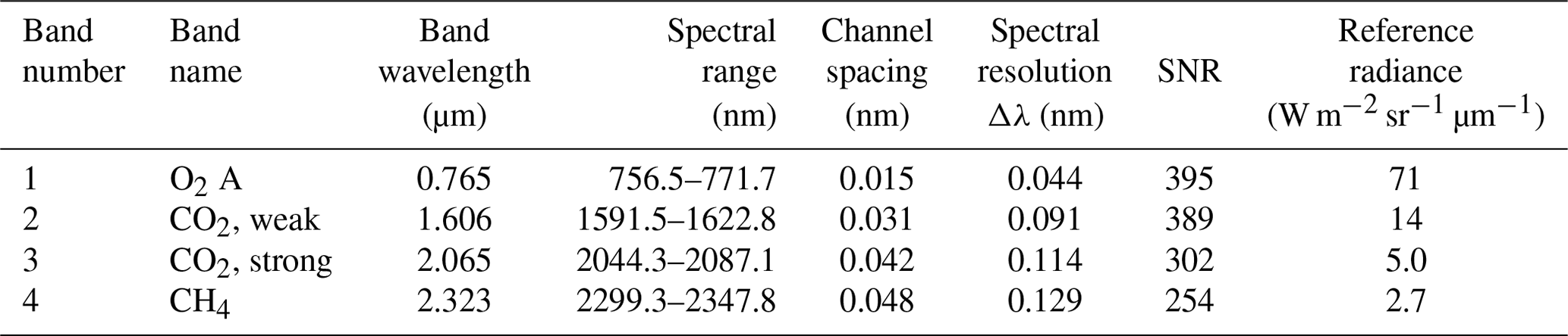
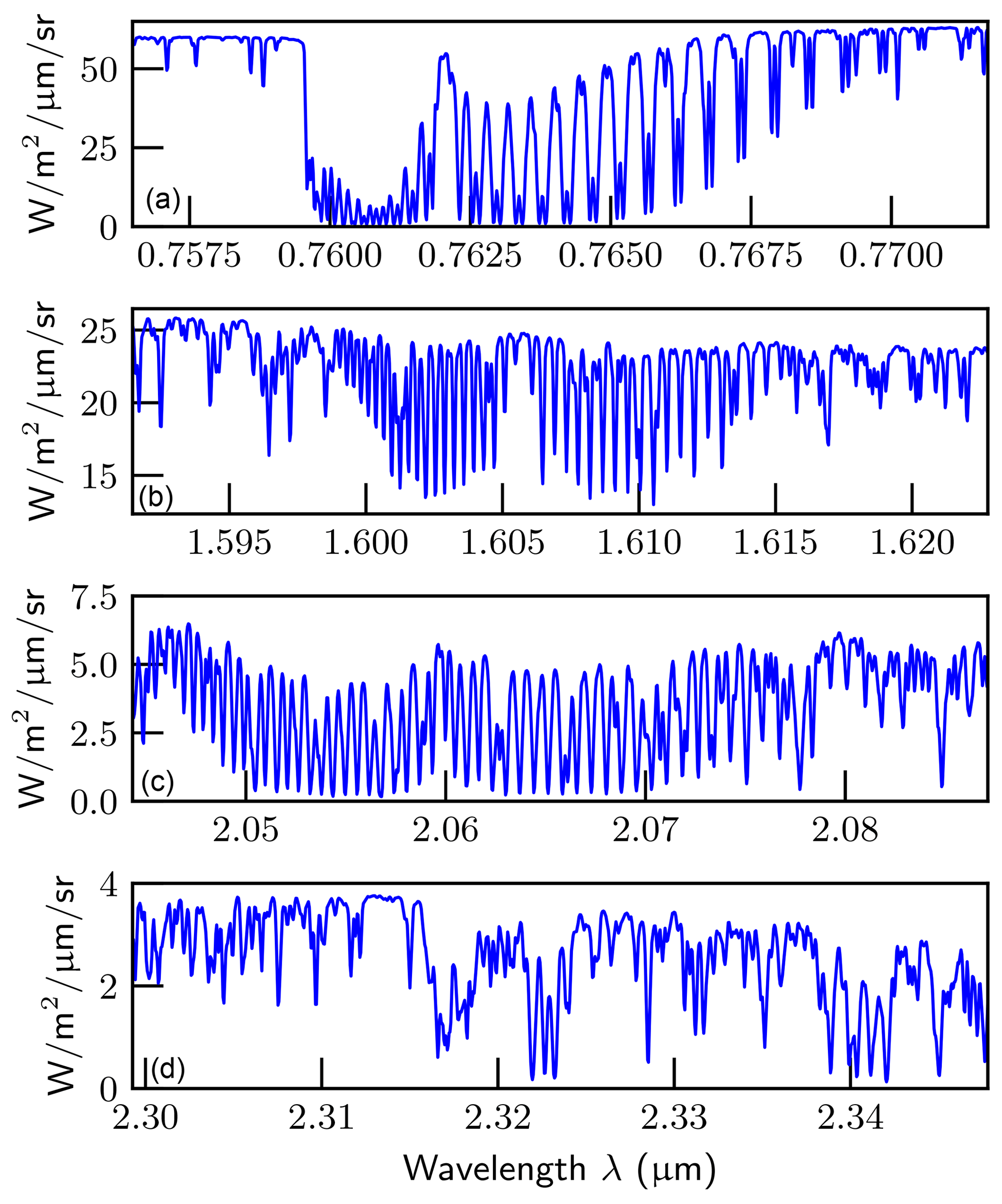
Figure 1 Sample spectra of observed radiance from a typical air mass scenario. Panels include, from (a) to (d), the O₂ A, weak CO₂, strong CO₂, and CH₄ bands, respectively.

The current set of satellite missions capable of measuring atmospheric greenhouse gas concentrations, including OCO-2, OCO-3, GOSAT-1, GOSAT-2, and TROPOMI, are all in polar orbits that cover most or all of the Earth's surface but only with a limited temporal sampling. GeoCarb was the first planned geostationary Earth observation mission for measuring greenhouse gases and SIF, distinguishing it from the current suite of polar orbiting GHG missions. In a geosynchronous orbit, with its configurable imaging/mapping capability, it will be able to measure $X_{{\mathrm{CO}}_{\mathrm{2}}}$, $X_{{\mathrm{CH}}_{\mathrm{4}}}$, and X_CO at the urban to continental scales and at the spatial and temporal resolutions that are sufficient enough to resolve emission sources and significantly improve land–atmosphere CO₂ and CH₄ flux calculations and reduce the uncertainty of these fluxes. Hence, GeoCarb is capable of acquiring multiple observations of the same location per day for most of the western Hemisphere. Since GeoCarb is not configured to make ocean glint observations regularly, retrievals over ocean will not be made operationally.

The GeoCarb scan strategy will include a set of scan blocks that cover most of the land surfaces of North, South, and Central America, up to three times a day. The scan strategy will minimize overlap between blocks and observations over ocean and will be optimized for signal-to-noise ratio (SNR) with respect to solar zenith angle and air mass factor. The scan blocks are configurable in location, size, and frequency. This allows GeoCarb to alter its scan strategy to intensively scan smaller regions of particular interest or uncertainty many times a day, for detailed emission estimates, for calibration and validation, or for transient events in a campaign mode. The scan strategy has yet to be formalized, although proposed strategies have been published in the literature (Nivitanont et al., 2019b; Somkuti et al., 2021).

GeoCarb is equipped with a four-band spectrometer with two arms. The shortwave (SW) arm covers the O₂ A-band (0.765 µm) and the weak CO₂ band (1.606 µm), and the longwave (LW) arm covers the strong CO₂ band (2.065 µm) and the CH₄/CO band (2.323 µm). Light is first incident on two orthogonally oriented scan mirrors used for pointing. This light is then transmitted to a three mirror anastigmat telescope with a 54 mm entrance aperture and a 4.3^∘ field of view (FOV), forming a well-corrected image on an 18 mm × 0.042 mm spectrometer entrance slit. Following the slit, a dichroic beamsplitter separates the SW and LW channels to the two arms of the spectrometer, each with a single echelle grating used in two orders. Additional dichroic beamsplitters direct the light to one of the focal plane assemblies (FPAs) specific to each band with a narrowband order sorter filter ahead of the FPAs. The FPAs are HgCdTe detectors with 1016 × 1016 active pixels, with the spatial direction along columns and the dispersion direction along rows.

The slit is projected on the Earth with the spatial dimension oriented north–south (N–S). The angular size of the slit is 4.3^∘ in the along-slit direction and 0.00833^∘ in the across-slit direction. At the SSP, this is 25^∘ in latitude or 2800 km N–S on the surface of the Earth. Given the 18 mm × 0.042 mm size of the slit and the 1016 samples of the FPA distributed along-slit, the angular resolution for a single footprint is approximately 123 µrad along-slit at nadir. At the geostationary altitude of 35 786 km, this results in a footprint size of approximately 2.7 km along-slit (at the slit center, increasing by 2.4 % toward the slit ends because of Earth curvature) and 5.4 km across-slit at nadir. The slit is pointed utilizing the two orthogonally oriented scan mirrors, a N–S scan mirror that can be rotated a total of ±3.55^∘ and an E–W scan mirror that can be rotated a total of ±5.00^∘. These mirrors are capable of pointing the slit over a range of 20^∘ in the N–S direction and 18.5^∘ in the E–W direction, respectively, which covers the Earth disc with a diameter of 17.4^∘ viewed from the geostationary orbit. For each scan block the E–W scan mirror will move in equiangular steps in a step-and-stare mode with 0.3825 s per step and 9.0 s per stare (integration time). The E–W scan rate is 2.7 km per 4.4625 s = 2178 km h⁻¹, so that continental width scans are completed in 1.5 to 3 h.

Due to GeoCarb's step-and-stare scanning method and high spectral resolution, the instrument is sensitive to across-slit scene inhomogeneity. In the context of greenhouse gas measurements, this has been discussed by several authors (Landgraf et al., 2016; Meister et al., 2017; Nivitanont et al., 2019a). In particular, the effective instrument ILS will vary across a FOV depending on the scene brightness inhomogeneity within the FOV. One method of mitigating this effect is by installing a slit homogenizer into the optical assembly effectively smearing out the inhomogeneity across the FOV. Due to schedule constraints during instrument assembly, the decision was made to remove the homogenizer and replace it with an air slit. Another mitigation method, and currently planned for GeoCarb, is to fit for an ILS scaling factor for each band in the L2 retrieval, effectively scaling the FWHM, which will either stretch or squash the ILS making it broader or narrower, therefore optimizing the ILS for each FOV.

There are several other instrument-related uncertainties that occur in the GeoCarb instrument that are under investigation to understand their effects and to develop rectification methods for those effects in either the measured radiances or in the retrievals. These include “smile”, the keystone effect, stray light, and detector persistence.

Calibrated, spectrally resolved radiances for each of the four bands will be distributed in level-1B (L1B) files which also contain the measurement's geolocation, solar and satellite geometry, instrument characteristics, and other parameters normally required to make use of the measurements. In addition, each L1B file will be distributed with a “Met” file that contains meteorological information required for the L2 retrievals.

3 Level-2 retrieval algorithm

The GeoCarb L2 retrieval algorithm code, also known as L2 full–physics (L2FP), is a fork of the L2FP code developed at the NASA Jet Propulsion Laboratory (JPL) since 2004 for OCO and then subsequently for GOSAT (2009), OCO-2 (2014), and OCO-3 (2019) (Connor et al., 2008; O'Dell et al., 2012; Crisp et al., 2012; O'Dell et al., 2018). Development of the GeoCarb fork maintains backward compatibility with the OCO-2/3 base, which means that not only can it be used for the same instruments as the JPL code base but also that improvements made to the JPL code are merged into the GeoCarb code base. In this section an overview of the retrieval algorithm is given, with a focus on changes made to the GeoCarb code base relative to the OCO-2/3 code base in detail.

3.1 Inversion

The inversion methodology used in the GeoCarb L2FP retrieval is based on the OE approach for atmospheric inverse problems described by Rodgers (2004) in which input parameters to a forward model are optimized to obtain the best match between real measurements and simulated measurements output from a forward model while being constrained by a priori knowledge of the input parameters. This relationship is given by

$$\begin{array}{}\text{(2)}& \mathit{y}=\mathbf{F}(\mathit{x},\mathit{b})+\mathit{ϵ},\end{array}$$

where F is the forward model, x is the n element input state vector containing the input parameters to be optimized, y is the m element measurement vector containing the calibrated radiance spectra for all four bands ($m=\mathrm{4}\times \mathrm{1016}$), b is the set of all other assumed model parameters not in the state vector x, and ϵ represents the measurement and forward model error. The inverse solution for the optimized state vector $\widehat{\mathit{x}}$ is obtained by minimizing a cost function which can be expressed as a χ² distribution given by

$$\begin{array}{}\text{(3)}& \begin{array}{rl}{\mathit{\chi }}^{\mathrm{2}}& ={\left[\mathit{y}-\mathbf{F}(\mathit{x},\mathit{b})\right]}^{\mathrm{T}}{\mathbf{S}}_{\mathit{ϵ}}^{-\mathrm{1}}\left[\mathit{y}-\mathbf{F}(\mathit{x},\mathit{b})\right]\\ & +(\mathit{x}-{\mathit{x}}_{\mathrm{a}}{)}^{\mathrm{T}}{\mathbf{S}}_{\mathrm{a}}^{-\mathrm{1}}(\mathit{x}-{\mathit{x}}_{\mathrm{a}}),\end{array}\end{array}$$

where S_ϵ is the measurement and forward model error covariance matrix, x_a is the a priori state vector, and S_a is the a priori error covariance matrix. x_a and S_a denote the best guess of the state before the measurement is made and the uncertainty of this guess, respectively.

The retrieval problem is ill-posed leading to non-existence, non-uniqueness (due to discretization of the problem), and/or ill-conditioning (due to amplification of errors in x due to errors in y). It is for this reason that an a priori constraint is required. The fact that the problem is nonlinear requires an iterative method. Finally, in order to perform the iteration efficiently, while maintaining a stable step size, a form of regularization is required. To satisfy these requirements the Levenberg–Marquardt (Levenberg, 1944; Marquardt, 1963) method is applied to Gauss–Newton iteration (Rodgers, 2004; Connor et al., 2008).

After successful convergence an estimate of the a posteriori covariance matrix $\widehat{\mathbf{S}}$ is computed. Several other information and diagnostic quantities are also produced and included in the L2FP product, including the averaging kernel matrix A and the number of degrees of freedom for signal d_s. See Connor et al. (2008) for a full description of the quantities.

3.2 Forward model

The forward model $\mathit{y}=\mathbf{F}(\mathit{x},\mathit{b})$ simulates the measurements in y and analytically computes the derivatives in the matrix K with respect to the state vector parameters. Most of the current forward model has been described in detail by O'Dell et al. (2012, 2018) in the context of the OCO-2 mission and is only described briefly in this section. However, there are some instrument model changes specific to GeoCarb which include noise, polarization, and the ILS.

The forward model can be broken down into several sub-models: an atmospheric model; a gas absorption model; an aerosol model; a surface model; a solar model; a radiative transfer (RT) model; and, finally, an instrument model. The atmospheric model discretizes the atmosphere into 20 layers using a sigma-pressure level system where the pressure levels scale with surface pressure and the topmost level is at 0.01 hPa. Parameters including temperature and humidity, trace gas concentrations, and aerosol/cloud concentrations are defined on each level by their various models from which the wavelength-dependent layer quantities required for the RT computations are computed along with a layer at the bottom for the atmosphere for surface reflectance. All but the instrument model are explained in detail in the references cited and will not be reiterated here. Here we will focus on the instrument model in the context of GeoCarb.

3.2.1 Instrument model

The instrument model consists of three components: (1) a polarimetric model, (2) an instrument line shape (ILS), and (3) a noise model which are described below. Note that the other instrument effects discussed in Sect. 2 are not accounted for in the instrument model presented and therefore are ignored in this study.

Polarimetric model

The polarimetric model predicts the intensity that is eventually incident on the detectors after being transmitted through the scan mirrors, telescope, beam splitter, and gratings. The polarization effects of each of the optical components can be linearly combined into a single-wavelength-dependent Mueller matrix, as shown in O2015. The intensity is computed with a simple matrix transformation on the Stokes vector $\mathit{S}\left(\mathit{\lambda }\right)=\left[I\right(\mathit{\lambda }),Q(\mathit{\lambda }),U(\mathit{\lambda }),V(\mathit{\lambda }\left)\right]$ incident on the scan mirrors by the 4×4 Mueller matrix M(λ) for which the wavelength dependence is linear across each band:

$$\begin{array}{}\text{(4)}& I_{b,i}={\mathbf{M}}_{b,\mathrm{0}}{\mathit{S}}_{b,i}+{\mathbf{M}}_{b,\mathrm{1}}{\mathit{S}}_{b,i}({\mathit{\lambda }}_i-{\mathit{\lambda }}_{\mathrm{0}}),\end{array}$$

where I_b,i is the radiance for band b, at the high resolution grid point i; M_b,j is the 1×4 Mueller matrix for band b and linear dependence order $j=\mathrm{0},\mathrm{1}$; and S_b,i is the Stokes vector. The four elements of the Mueller matrix, often called the Stokes coefficients, are $m_{\mathrm{00},b,j}$, $m_{\mathrm{01},b,j}$, $m_{\mathrm{02},b,j}$, and $m_{\mathrm{03},b,j}$ and are determined during pre-flight polarimetric calibration. It should be noted the last element of the Stokes vector is typically small as the surface and atmosphere generate very little circular polarization; therefore, to save processing time, the RT is computed using only the first three elements of the Stokes vector and a 1×3 Mueller matrix. Finally, we note that for GeoCarb, Eq. (4) can be written in a simplified form as

$$\begin{array}{}\text{(5)}& \begin{array}{rl}{I}_{b,i}& =I\left({\mathit{\lambda }}_i\right)+\left[c_{\mathrm{0}}+c_{\mathrm{1}}({\mathit{\lambda }}_i-{\mathit{\lambda }}_{\mathrm{0}})\right]\\ & \times \left(Q\left({\mathit{\lambda }}_i\right)\cos \mathrm{2}{\mathit{\varphi }}_{\mathrm{p}}-U\left({\mathit{\lambda }}_i\right)\sin \mathrm{2}{\mathit{\varphi }}_{\mathrm{p}}\right),\end{array}\end{array}$$

where c₀ and c₁ are primarily functions of the grating efficiency as a function of wavelength in each band, and ϕ_p represents the angle between the axis of vertical polarization (with respect to the grating) and the reference plane for polarization. Both Stokes components Q and U also depend upon the chosen reference plane for polarization. We follow the OCO-2/3 convention and choose the local meridian plane to be this reference plane for polarization, which is the plane containing the local normal unit vector and the vector pointing from the target FOV to the satellite. For further details, see O2015.

ILS convolution

The radiance measured in each of the 1016 spectral channels, of each of the four bands, for each of the 1016 footprints along the slit, is the result of the convolution of intensity computed on a high-spectral-resolution (0.01 µm) spectral grid with an instrument spectral response function:

$$\begin{array}{}\text{(6)}& I_{\mathrm{f},\mathrm{b},\mathrm{c}}=\underset{{\mathit{\lambda }}_{\mathrm{0}}}{\overset{\mathrm{\infty }}{\int }}{I}_{\mathrm{f},\mathrm{b},\mathrm{i}}{\mathrm{ILS}}_{\mathrm{f},\mathrm{b},\mathrm{c}}\left(\mathit{\lambda }\right)\mathrm{d}\mathit{\lambda },\end{array}$$

where $I_{\mathrm{f},\mathrm{b},\mathrm{c}}$ is the radiance for footprint “f”, band “b”, and channel “c”; $I_{\mathrm{f},\mathrm{b},\mathrm{i}}$ is the radiance for footprint “f”, band “b”, and high-resolution grid point “i”; and ${\mathrm{ILS}}_{\mathrm{f},\mathrm{b},\mathrm{c}}\left(\mathit{\lambda }\right)$ is the footprint-, band-, and channel-dependent ILS as a function of wavelength λ. In practice, the integration is performed over a limited range centered on each channel of 0.00082, 0.0022, 0.0028, and 0.0025 cm¹ for bands 1, 2, 3, and 4 respectively.

Radiometric noise model

The instrument noise model is used to build the measurement and forward model error covariance matrix S_ϵ. In addition, for the retrieval simulation experiments presented in Sect. 4, the noise model is used to add synthetic noise to the simulated measurements. The noise model will ultimately be based on laboratory measurements, although for this study the model (of the same form) is based on theory, but we expect that the outcome of the experiments presented will not change significantly with the final noise model based on measurements. The standard deviation of noise ${\mathit{\sigma }}_{I_{\mathrm{b},\mathrm{c}}}$ for band “b” and channel “c” is given by

$$\begin{array}{}\text{(7)}& {\mathit{\sigma }}_{I_{\mathrm{b},\mathrm{c}}}=\sqrt{n_{\mathrm{0},\mathrm{b},\mathrm{c}}^{\mathrm{2}}+n_{\mathrm{1},\mathrm{b},\mathrm{c}}{I}_{\mathrm{b},\mathrm{c}}},\end{array}$$

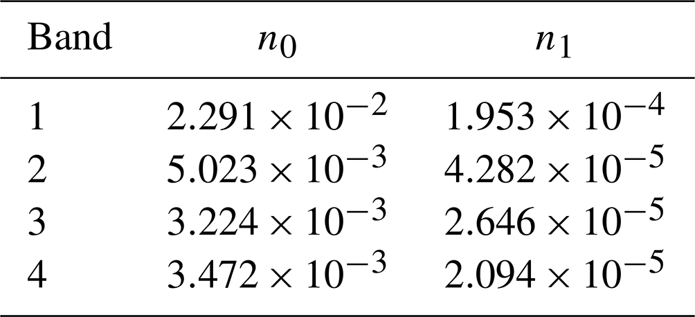
where $n_{\mathrm{0},\mathrm{b},\mathrm{c}}^{\mathrm{2}}$ is the background noise coefficient, $n_{\mathrm{1},\mathrm{b},\mathrm{c}}$ is the coefficient for noise proportional to the radiance (shot noise) I_b,c, and the radiance and the coefficients are in units of W m⁻² sr⁻¹ µm⁻¹. Unlike the ILS, the instrument noise is independent of the footprint “f” along the slit but does vary (roughly quadratically) with wavelength in each band. Table 3 gives the mean noise coefficients for each band used in this study. Like the other instrument parameters, noise coefficients will be determined during preflight calibration.

Table 3 GeoCarb noise coefficients used in this study, in units of W m⁻² sr⁻¹ µm⁻¹.

3.3 State vector and a priori

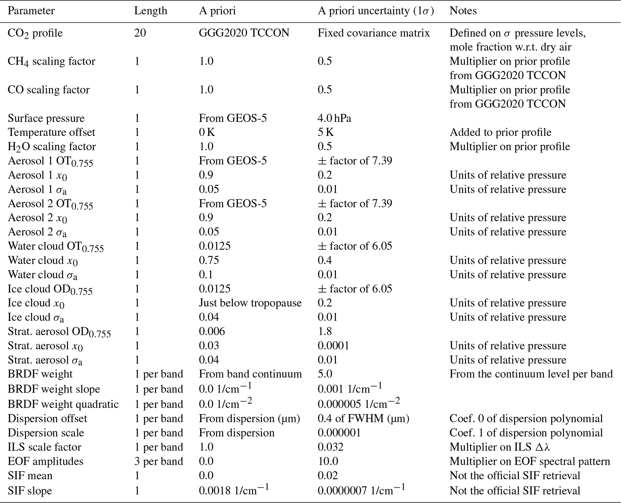
The state vector x contains the parameters that are optimized during the inversion process. The parameters include values that are used to compute the retrieval values of $X_{{\mathrm{CO}}_{\mathrm{2}}}$, $X_{{\mathrm{CH}}_{\mathrm{4}}}$, and X_CO, in addition to other parameters that are sensitive to the measurements but are not known perfectly, such as meteorological, aerosol/cloud, surface, and instrument-related parameters. Much of the state vector is described in detail by O'Dell et al. (2012, 2018). Here the state vector elements are discussed focusing in detail on elements added for GeoCarb. In total there are n=78 fitted parameters in the state vector. The prior values used for these parameters are also described, as are their associated error covariances. Table 4 presents the state vector, along with the priors and associated 1σ uncertainties.

CO₂ is represented in the state vector as a profile of dry-air mole fraction on the forward model's 20 sigma-pressure levels. CH₄ and CO profile retrievals are typically limited to ∼1 degree of freedom for signal d_s, so for GeoCarb a scaling retrieval is performed for these gases, where the prior profile is scaled by a single retrieved parameter with a prior value of unity. The prior CO₂, CH₄, and CO profiles are nearly identical to those used in the GGG2020 TCCON retrieval (Wunch et al., 2017) produced as described in Laughner et al. (2023). The CO₂ prior covariance matrix is constructed such that the total prior uncertainty of $X_{{\mathrm{CO}}_{\mathrm{2}}}$ is 12 ppm, a value somewhat larger than natural variability, that gives more weight to the measurements relative to the prior. The prior uncertainties for the CH₄ and CO scale factors are both set to 0.5.

Table 4 GeoCarb state vector and a prior (see Table 2 in O'Dell et al., 2018, for a full description of the parameters and comparison to the OCO-2/OCO-3 state vector).

Meteorological quantities included in the state vector are surface pressure, a temperature profile offset, and a water vapor profile multiplier. Surface pressure is included to account for path length modification effects and other systematic errors common to the absorption bands used in the retrieval. The temperature and water vapor profiles both affect trace gas absorption, while water vapor is in itself an important absorber across all four bands. The prior surface pressure and temperature and water vapor profiles are obtained from the Goddard Earth Observing System Data Assimilation System (GEOS-5) Forward Processing for Instrument Teams (FP-IT) forecast (Rienecker et al., 2008; Lucchesi, 2013). The prior uncertainties of surface pressure, the temperature profile offset, and the water vapor scale are set to 4 hPa, 5 K, and 0.5, respectively.

For particles, two tropospheric aerosol types, liquid water cloud and ice cloud, and a stratospheric aerosol are included in the state vector including their density x₀, the 1σ profile width σ_a, and the natural logarithm of the optical thickness (OT) at 0.755 µm ln(OT_0.755). For each sounding the two tropospheric aerosol types with the highest values of OT_0.755 based on the GEOS-5 FP-IT aerosol forecast are chosen.

The surface bidirectional reflectance distribution function (BRDF) amplitude weight, weight slope, and weight quadratic terms are included in the state vector for each band. The prior weight values are estimated directly from the level of the continuum in the observed spectrum of each band, assuming a clear-sky, absorption-free atmosphere, and prior slopes and quadratic parameters are set to zero. The corresponding prior uncertainties are set to sufficiently large values so that the amplitude parameters are essentially unconstrained.

The dispersion scale and offset coefficients are included in the state vector for each band. The prior values are simply set to zero and 1, respectively, of the dispersion polynomial for each band. The prior uncertainties for the offset are set to 0.4 times the FWHM for each band and for the scale are set to 10⁻⁶ for each band.

To mitigate the effects of the scene inhomogeneity on the ILS across the scene, an ILS scaling factor is fitted for each band effectively scaling the FWHM. The prior scaling is set to unity with a prior uncertainty of 0.032 for each band.

Spectral residuals, the difference between the measured radiance and the modeled radiance from the retrieved state vector, contain systematic structure due to unknown spectroscopic errors, solar model errors, and instrument characteristics. To account for these residuals, empirical orthogonal functions (EOFs) are created from a clear-sky training dataset to represent the spectral patterns, for which amplitude factors are included in the state vector and fitted for per band and per EOF. The prior amplitude factors for each band are set to zero, with prior uncertainties of 10.0 each.

To account for the effects of SIF emission from the vegetation on the surface two SIF parameters are fitted for: a mean and a slope across the O₂ A-band. It is important to note that the SIF parameters in the state vector are not the official GeoCarb SIF product which is produced by the Generic Algorithm for the Single Band Acquisition of Gases (GASBAG) briefly introduced in Sect. 3.5.2 and discussed in detail by Somkuti et al. (2021). The prior SIF mean is set to zero and the prior slope is set to 0.0018 1/cm⁻¹ while the associated uncertainties are set to 0.02 and 7⁻⁷ 1/cm⁻¹, respectively.

3.4 Measurement vector and error covariance

The measurement vector y contains the radiance measurements with length m=4 bands × 1016 channels. For the m×m measurement and forward model error covariance matrix S_ϵ, it is assumed that there is no error correlation between channels, so as a result it is diagonal, such that $S_{\mathit{ϵ},\mathrm{b},\mathrm{c},\mathrm{c}}={\mathit{\sigma }}_{{\mathrm{I}}_{\mathrm{b},\mathrm{c}}}^{\mathrm{2}}$, where ${\mathit{\sigma }}_{I_{\mathrm{b},\mathrm{c}}}$ is from the noise model given by Eq. (7). In the GeoCarb retrieval, as is common in many retrievals, the forward model error is not included due to the difficulty of characterizing this error, which is assumed to be significantly less than the measurement error.

3.5 Pre-screening

Soundings that are unlikely to produce reliable L2FP results are filtered out. This is important since, due to the large number of channels per sounding ($\mathrm{4}\times \mathrm{1016}=\mathrm{4096}$ total channels), the L2FP algorithm is rather computationally intensive. This, combined with the relatively large number of observations made on a daily basis, results in a significant computational burden. Therefore it is advantageous to avoid running it on soundings unnecessarily.

The first step in pre-screening is to of course skip soundings that are flagged as having radiances or supporting fields that are missing due to instrumental anomalies or L1B processing issues. Since the signal from soundings over ocean surfaces is too low to perform a successful retrieval and GeoCarb does not have a operational sun-glint mode, these scenes will not be processed. Ocean surfaces are identified using the land/water mask contained in the L1B file which is populated using the International Geosphere–Biosphere Programme (IGBP) land classification database (Townshend, 1992). Finally, soundings with aerosols and clouds that are too thick to produce a useful retrieval are filtered out. Aerosol and cloud filtering is performed using results from the A-band preprocessor (ABP) and the Generic Algorithm for the Single Band Acquisition of Gases (GASBAG), each discussed in the next two sections, respectively. The filtering is conservative, so that inevitably there will be scenes where the aerosol/cloud still might be too thick to yield a useful retrieval that will most likely be filtered out in the post-processing filtering discussed in Sect. 3.6.

Table 5 Scan blocks that are used in the retrieval simulation experiments. Fields include the scan block number, name, size in the x and y directions N_x and N_y, the total number of soundings, minimum and maximum latitude/longitude at the middle of the scan block in the $x/y$ directions, and the UTC times associated with the start and the end of the east–west scan of the north–south-oriented slit.

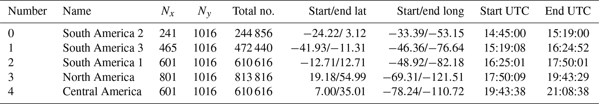
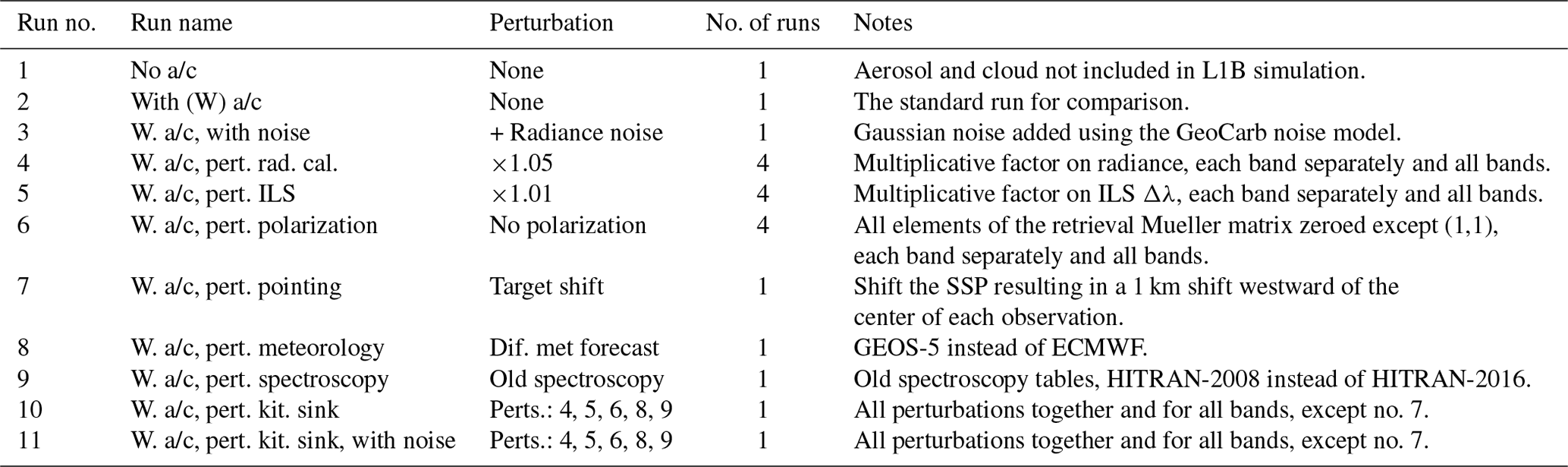
Table 6 The experimental runs with or without aerosol/cloud (a/c), with or without noise, and with the given perturbations (pert.) applied on the baseline run.

3.5.1 A-band preprocessor

The A-band preprocessor (Taylor et al., 2012) performs an O₂ A-band retrieval using a fast forward model and assuming no aerosol or cloud, only molecular scattering. The spectrum is fit to the clear-sky model with five free parameters: surface pressure P_s, an offset to the meteorological temperature profile, a spectral dispersion offset, and the surface albedo at the two band endpoints. Two quantities are then defined upon which to filter: ΔP_s,cld is the retrieved minus a priori surface pressure, and ${\mathit{\chi }}_R^{\mathrm{2}}$ is the ratio of the fit χ², relative to the minimum χ² value possible at that same SNR. Scenes with $\left|\mathrm{\Delta }{P}_{\mathrm{s},\mathrm{cld}}\right|>\mathrm{40}$ hPa or ${\mathit{\chi }}_R^{\mathrm{2}}>\mathrm{2.3}$ are flagged as cloudy. The thresholds are set to be loose to filter only scenes where the aerosol/cloud is obviously too thick.

3.5.2 Generic Algorithm for Single-Band Acquisition of Gases

The Generic Algorithm for Single-Band Acquisition of Gases (Somkuti et al., 2021) performs retrievals of SIF and is the main processor for the GeoCarb operational SIF product L2GSB. In addition, it produces the so-called ratio retrievals which are used for aerosol and cloud screening, where independent single-band retrievals of $X_{{\mathrm{CO}}_{\mathrm{2}}}$ and $X_{{\mathrm{H}}_{\mathrm{2}}\mathrm{O}}$, in both the weak CO₂ and strong CO₂ bands, are obtained by retrieving scaling coefficients of the prior gas profiles for both CO₂ and H₂O gases. Calculating the ratio of $X_{{\mathrm{CO}}_{\mathrm{2}}}$ and $X_{{\mathrm{H}}_{\mathrm{2}}\mathrm{O}}$ between the values retrieved in both bands yields a value for each gas. In a completely cloud- and aerosol-free atmosphere, the value will be close to unity. When aerosols and clouds are introduced, the photon path length can be different between the retrieval bands, as they are separated by roughly 0.4 µm. Since the retrieval approach is non-scattering, the only way for the forward model to adjust to the scattering-induced change in observed line depths is to scale the gas profiles, which ends up changing the ratio to be different from unity. Thus, the gas ratio provides an indicator for cloud and aerosol contamination in a measurement. The minimum and maximum ratio thresholds are currently set to 0.8 and 1.5, respectively, for both gases.

3.6 Post-processing

The pre-screening filters out soundings with aerosols and clouds that are too thick from which to yield a useful retrieval but is aerosol/cloud-conservative, so there will be some soundings that still contain a small amount of aerosol and cloud. Of the soundings that pass the pre-screening and are processed with L2FP, some fail to converge. This could be due to the presence of thinner aerosols and clouds, limitations in the forward model to model the observed radiances with sufficient accuracy, and/or the fact that the inversion problem is ill-posed and nonlinear by nature, making it difficult sometimes to optimally minimize χ². Subsequently, there will be retrievals with X_gas results that have errors larger than expected compared to the 1σ a posterior uncertainty from the retrieval due to scatter and/or systematic bias. A quality filtering procedure attempts to remove these problematic soundings. This is followed by a linear bias correction of systematic errors to remove spurious dependencies in some variables on the retrieval. Both the filtering and bias correction steps essentially follow the methods described in O'Dell et al. (2018).

3.6.1 Filtering

Building filters is accomplished by selecting a training dataset and finding the variables that have the largest influence on the dataset by evaluating

$$\begin{array}{}\text{(8)}& \mathrm{\Delta }{X}_{\mathrm{gas}}=X_{\mathrm{gas},\mathrm{ret}}-X_{\mathrm{gas},\mathrm{true}},\end{array}$$

where X_gas,ret is the retrieved X_gas, and X_gas,true is what is considered the true X_gas. For an operational instrument the truth is obtained from one or more truth proxies which can be ground-based observations, such as TCCON, or carbon flux inversion models. For a simulation study such as this one, the truth is computed from the measurement simulation inputs themselves, after applying the averaging kernel correction. The filtering is performed for $X_{{\mathrm{CO}}_{\mathrm{2}}}$, $X_{{\mathrm{CH}}_{\mathrm{4}}}$, and X_CO together, ensuring a consistent set of filtered soundings for each gas. Variables from L2FP, ABP, and GASBAG are all subject to being used in a filter threshold and include not only state vector variables but variables derived from the retrievals. It is important to note that the optimal filter is not static. Changes in L2FP inputs, such as radiances (due to calibration changes), spectroscopic updates, updates in the meteorological modeling, and changes to the L2FP algorithm itself, will most likely require the production of a new set of filters. This burden will subsequently be shown in this paper including the fact that this process can be a bit tedious but, as it turns out, that the process conveniently lends itself to machine learning techniques which are under investigation (Keely et al., 2021).

3.6.2 Bias correction

The bias correction contains two terms: a parametric bias correction and a global bias correction. The bias correction for a particular sounding i is given as

$$\begin{array}{}\text{(9)}& X_{i,\mathrm{gas},\mathrm{flt},\mathrm{bc}}=X_{i,\mathrm{gas},\mathrm{flt}}-C_{\mathrm{p}}-C_{\mathrm{g}},\end{array}$$

where $X_{i,\mathrm{gas},\mathrm{flt}}$ is the filtered X_gas for sounding i, C_p is the parametric correction term, and C_g is the global correction term. The parametric bias correction has the form of a multiple linear regression following Wunch et al. (2011b):

$$\begin{array}{}\text{(10)}& C_{\mathrm{p}}=\sum _j^n{c}_j(p_j-p_{i,\mathrm{ref}}),\end{array}$$

where c_j are the regression coefficients, p_j are the selected parameters, and p_i,ref are the parameter reference values. The parameters used are those that remove greater than 5 % of the variance relative to the global mean of the same truth proxies used to construct the filters. As with the filters, for this study the simulation inputs are used as the truth, after the averaging kernel correction is applied. The set of parameters identified may be different with X_gas. It is important to note that, just as with the filters, the optimal set of parameters used for the parametric bias correction is not static and changes with changes in the input data and the algorithm. The global bias correction is simply the median difference between a sample set of filtered X_gas results and a matching sample set of true X_gas values from the truth proxy:

$$\begin{array}{}\text{(11)}& C_{\mathrm{g}}=\mathrm{median}({\mathit{X}}_{\mathrm{gas},\mathrm{flt}}-{\mathit{X}}_{\mathrm{gas},\mathrm{true}}),\end{array}$$

where X_gas,flt and X_gas,true are vectors whose elements are the set of samples.

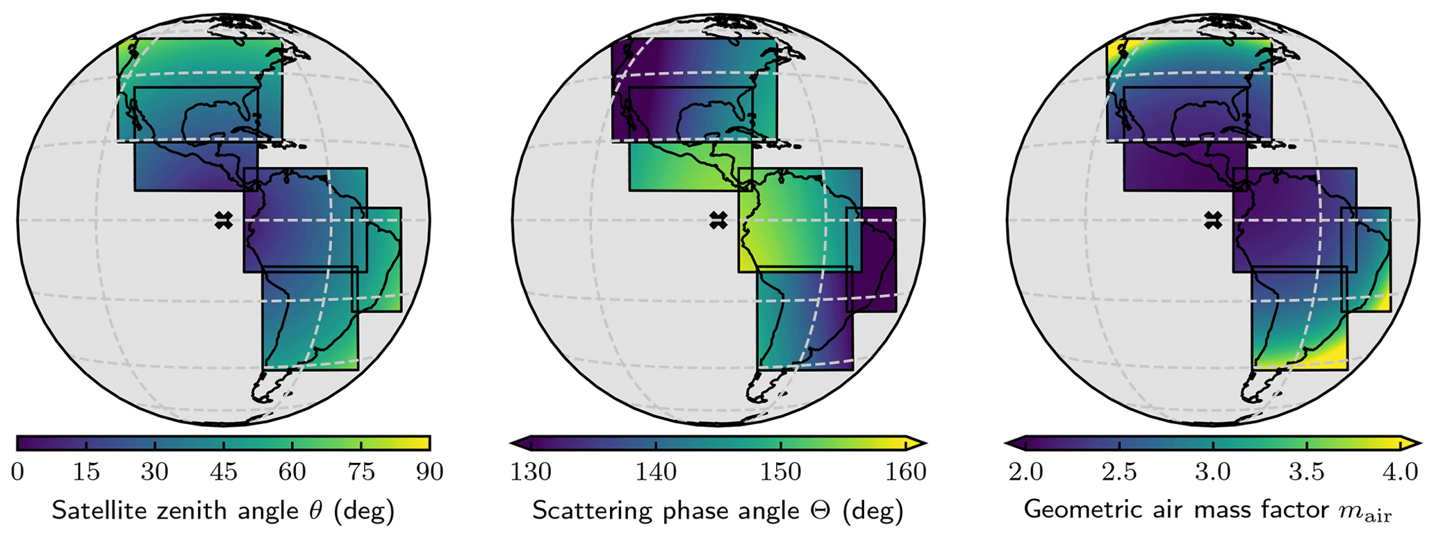
Figure 2 Maps of three key retrieval input variables for 21 June 2016 plotted in the five scan blocks used for the retrieval simulation experiments. The “X” at the center of the geostationary projection shows the GeoCarb sub-satellite point at 87^∘ west.

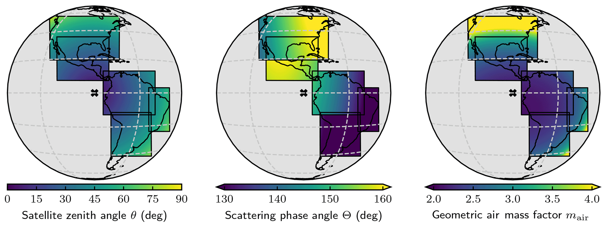
Figure 3 Same as Fig. 2 but for 21 December 2016.

4 Retrieval simulations and perturbation analysis

Up to this point, we have described the instrument, retrieval algorithm, pre- and post-filtering, and bias correction strategy of the retrieval approach. These are elements common to most other retrievals for GHGs and more generally remotely sensed variables. In this section, we apply it to GeoCarb more specifically, to investigate how imperfect knowledge of several important parameters affects the L2 retrievals. To this end, bottom-up retrieval simulations with perturbations on those parameters were performed. We start by describing our scan strategy in Sect. 4.1, which yields a set of scenes that covers most of the Americas at the peak of each season. We then describe the Colorado State University (CSU) simulator in Sect. 4.2, which produces the L1B and Met files used in our retrieval experiments. Finally, the setup for each L2 retrieval experiment is described in Sect. 4.3, including details that are common to each experiment and, for each individual experiment, the perturbations made on the retrieval system inputs and other relevant details specific to the experiment.

4.1 Simulation scan strategy

Since a formal GeoCarb scan strategy has yet to be determined, for these retrieval experiments a simple strategy was created that consists of five scan blocks that cover the land in the full disc that will most likely be covered by GeoCarb. The SSP is set to 87^∘ west longitude, which gives good coverage of both North and South America. In total, 4 d of five scan blocks is included, 21 March, 21 June, 21 September, and 21 December 2016, each corresponding approximately to a seasonal equinox or solstice, for a total of 20 scan blocks. They cover most of the Americas with a highest and lowest latitudes at approximately 60 and −42^∘, respectively. The scan blocks are listed in Table 5, in the order in which they are scanned, including their number, name, size in the x and y directions, the total number of soundings, minimum and maximum latitude/longitude at the middle of the scan block in the $x/y$ directions, and the UTC times associated with the start and the end of the east–west scan of the north–south-oriented slit. The scan start times were picked to minimize the overall mean solar zenith angle and air mass for all five blocks together.

The scan blocks are illustrated in Figs. 2 and 3 for the 21 June and 21 December 2016 cases, respectively. Three maps of the Earth disc visible by GeoCarb at an SSP of 87^∘ west (marked by the thick black “X”) are shown. From left to right, the first shows the satellite zenith angle θ. It is clear that the satellite zenith angle increases radially away from the SSP or towards the outside of the Earth disc, which is inherent in a geostationary orbital configuration and a distinguishing characteristic from nadir-looking instruments such as OCO-2/3. This is important because the plane parallel assumption used in the RT in the retrieval forward model breaks down as the satellite zenith angle increases. The satellite zenith angles for scenes over land used in this study range from 7.54 to 78.06^∘. It is expected that, depending on other scene characteristics, aerosol optical thickness, and air mass path, scenes with larger satellite zenith angles will more likely be candidates to be filtered.

Analogously, large solar zenith angles are also problematic in the RT calculations. The solar zenith angle for GeoCarb scenes will depend on a combination of location and time, with earlier or later local observation times having larger solar zenith angles. It is important that the finalized scan strategy is optimized by minimizing the mean solar zenith angle. In contrast, since OCO-2 is in a sun-synchronous orbit, the solar zenith angles for OCO-2 observations are usually relatively low and consistent.

The second map from the left shows the single-scattering phase angle Θ of single-scattered photons reaching the instrument, which, by the spherical law of cosines, is given by the following relation:

$$\begin{array}{}\text{(12)}& \cos \mathrm{\Theta }=-\left[\cos {\mathit{\theta }}_{\mathrm{0}}\cos \mathit{\theta }+\sin {\mathit{\theta }}_{\mathrm{0}}\sin \mathit{\theta }\cos (\mathit{\varphi }-{\mathit{\varphi }}_{\mathrm{0}})\right],\end{array}$$

where θ₀ and θ are the solar and satellite zenith angles, and ϕ₀ and ϕ are the solar and satellite azimuth angles, both clockwise from north. The single-scattering phase angle is the input to the single-scattering phase function P(Θ), which is the distribution of scattering from a molecule or particle such that Θ=0^∘ is forward scattering and Θ=180^∘ is backscattering. In the backscattering case, the instrument would be viewing the so-called “hotspot”, but for GeoCarb, with the SSP over ocean (both at the currently planned 103^∘ west longitude and the 87^∘ used for this study), hotspot geometry will not be encountered for soundings over land. The phase angles for scenes over land used in this study range from 106.6 to 176.8^∘ and depend not only on location due to the satellite zenith angle but also on the observation time due to the solar zenith angle, which is apparent in the variation in phase angle with scan blocks scanned at different times.

Finally, the third map from the left shows the air mass factor m_air in a plane-parallel atmosphere given by

$$\begin{array}{}\text{(13)}& m_{\mathrm{air}}={\displaystyle \frac{\mathrm{1}}{\cos {\mathit{\theta }}_{\mathrm{0}}}}+{\displaystyle \frac{\mathrm{1}}{\cos \mathit{\theta }}}.\end{array}$$

The air mass factor is the direct optical path length of solar radiation incident at the top of the atmosphere (TOA) that is scattered once in the atmosphere or at the surface into a direct path back to TOA and measured by an instrument sensor, relative to the optical path for vertically incident and vertically scattered radiation, i.e., when cos θ₀=0 and cos θ=0. The air mass factor is important from a RT perspective in that as it increases, the plane-parallel assumption starts to break down increasing error in the forward model, while also the amount of aerosols and clouds in the direct path will increase, which increases the contribution of light reflected from aerosol/cloud in the upper troposphere relative to light reflected from the ground. This makes it less likely that the inversion will produce a useful retrieval passing the post-processing filters. In fact, the air mass factor itself is used as a filter variable (see Fig. 8) with a maximum threshold of 4.2. The air mass factors for the land scenes used in this study range from 2.01 to 13.00, indicating that at least some retrievals will not meet the maximum air mass factor threshold.

Due to the number of retrieval experiments performed, the current GeoCarb spatial resolution of 2.7 km N–S and 5.4 km E–W would be computationally prohibitive, so the resolution was down-sampled by a factor of 20 N–S × 10 E–W, ∼0.5^∘. Our goal is to study the retrieval system over a wide range of conditions, and we are not concerned about spatial coherence between neighboring pixels. Since the geographic range of our dataset covers that which GeoCarb would have sampled, we believe that even with the downsampling, our dataset will cover an adequate range of conditions. After downsampling, the number of soundings per season is 13 812 for a total of 55 248 soundings for all four seasons, which can be compared to the original numbers before downsampling of 2 752 344 per season for a total of 11 009 376 soundings.

4.2 CSU simulator

As input, the CSU simulator takes meteorological, trace gas, cloud and aerosol, and surface parameters for each individual scene based on location and time, along with instrument parameters, and produces L1B files which include synthetic radiometric measurements along with their time, geolocation, solar/satellite geometry, instrument characteristics, and other parameters associated with the measurements. In addition, the simulator produces Met files associated with each scene, which contain meteorological prior parameters that are used in the L2 retrievals. The simulator was originally developed for OCO-1, while support for OCO-2/3 and GOSAT was subsequently added, followed by support for GeoCarb. The simulator is discussed in detail in various references such as O'Brien et al. (2009) or P2014 and will only be summarized here.

The simulation process can essentially be divided into three steps:

1. Produce the geolocation and solar/satellite geometry for each scene based on scan block definitions including the starting epoch, SSP, target (scan block center) latitude/longitude, number of north–south (currently fixed at 1016 footprints along slit) and east–west FOVs, and north–south/east–west sample increment.

2. For each scene, from various sources, collect and interpolate the trace gas, meteorological, aerosol/cloud, and surface parameters for input into step three, referred to as the scene input, to produce “truth” Met files.

3. Take the information produced in steps one and two along with scene-independent instrument characteristics such as the Stokes coefficients, the ILS table, and noise coefficients to run the forward model that produces synthetic radiance measurements.

The simulator is well documented in O'Brien et al. (2009) and P2014. Changes relative to those references include updates discussed in Sect. 1 including the instrument model details discussed in Sect. 3.2.1. We would like to refer the interested readers to these references for further details. It should be noted that the simulator does not account for the other instrument effects discussed in Sect. 2. In addition, the effects of scene inhomogeneity are also not taken into account, and therefore ILS variation across the scene is ignored. In the end these effects will be important to rectify, for which there is ongoing research.

4.3 Experimental setup

In this section perturbation analysis experiments are presented, where perturbations are made on several key inputs to the L2 retrieval system. These perturbations will affect the entire system, including pre-processing (ABP and GASBAG), L2FP, and post-processing, and allow us to construct an error budget for GeoCarb given the uncertainties investigated (unmodeled effects notwithstanding). The following is an outline of the steps involved in producing results for each experiment.

1. Produce baseline L1B input with the CSU simulator on the full set of scenes that result from the scan strategy described in Sect. 4.1. This occurs before pre-processing so it includes scenes over ocean and scenes that will have too much aerosol/cloud to produce a reliable L2FP retrieval.

2. For each experiment perform the following steps:

   • a.

     If required, perturb one or more variables in the L1B input as appropriate.

   • b.

     Run pre-processing including filtering out scenes over ocean and running ABP and GASBAG and subsequently screening for clouds. Note that ABP and GASBAG results will also be used for the post-process filtering.

   • c.

     Run the L2FP retrieval with the perturbed inputs. Depending on the experiment, the perturbed inputs may be the L1B input and/or the spectroscopy and/or meteorology inputs.

   • d.

     Tailor and apply the post-process filtering and bias correction to the L2FP X_gas results.

   • e.

     Apply the averaging kernel correction to the truth for comparison to each experiment's results. The truth comes from the scene input to the RT component of the simulator.

   • f.

     Analyze the differences in X_gas between the truth and that retrieved by L2FP.

Since GeoCarb was not meant to perform retrievals over ocean, all soundings over ocean are filtered out for the L2 retrievals as discussed in Sect. 3.5. This process results in a reduction of the number of soundings to simulate to 8278 for each season for a total of 33 111 soundings. Since all but one of our experiments are performed with an atmosphere containing aerosols and clouds, the aerosol and cloud screening discussed in Sect. 3.5 is performed on all simulated soundings over land. This results in a further reduction in the number of soundings to perform retrievals on for each season to 3104 for a total of 12 520 soundings. Note that after the retrieval is performed, there will be an additional reduction in the number of retrievals used in the analysis due to the post-filtering discussed in Sect. 3.6.

There are a few differences in the L2FP runs for the experiments compared to the planned mission configuration presented in Sect. 3. At the time of this writing, the GeoCarb instrument has yet to undergo a formal instrument characterization of polarization, the ILS, or noise characteristics, so for the experiments in this study the Mueller matrix, the ILS, and the noise coefficients are based on known characteristics of the optical components and optical model calculations of the instrument as a whole. These make them particularly different from the truth fields, and hence the retrieval is truly challenged in this regard. For aerosol, the same aerosol types are used but the aerosol optical thickness prior comes from the aerosol climatology of the Modern-Era Retrospective analysis for Research and Applications (MERRA) (Rienecker et al., 2011). For the surface BRDF, the quadratic term is not included. Since the L1B simulations only include a linear variation in wavelength, leaving the quadratic term out in the L2FP retrievals will not affect the outcome of the experimental results. Finally, it was judged not to include EOFs for these experiments since for the baseline both the L1B simulations and the L2FP retrievals use the same spectroscopic tables, solar model, and instrument characteristics, and the effects of the perturbations applied in the experiments would be easier to decipher without the effects of applying EOFs. Therefore, we expect our results to be conservative, in that EOFs should only serve to reduce systematic errors (O'Dell et al., 2018).

4.3.1 Baseline experiments

To establish a “baseline” for comparison, we ran the retrieval system with nothing perturbed, i.e., with perfect knowledge of the experimental inputs. In this case, both the L1B simulations and the ABP, GASBAG, and L2FP retrievals use the same set of input parameters of interest. Even though these input parameters are the same, there are still differences in the simulator and L2FP that will result in X_gas retrieval errors relative to the “truth” computed from the simulator inputs. The differences include different aerosol/cloud models; different surface BRDF models; different SIF models; differences between the prior and truth profiles of CO₂, CH₄, and CO; differences in the layer discretization of the atmosphere; and subtle differences in the forward model RT. Errors relative to truth also arise from the OE inversion including the choice of additional priors and algorithmic controls and the ability for the algorithm to minimize the differences between the measurements and the forward model since the inversion problem is ill-posed and nonlinear by nature.

In addition to the baseline test described above, we performed two other tests with modifications to the baseline. First, the L1B simulator is ran without aerosols and clouds included. Although unrealistic, this test shows the effects of aerosols and clouds on the baseline test and on post-process filtering. In addition, baseline L1B files with synthetic noise added are produced, for the case including aerosols and clouds. This does not require a separate simulator run as synthetic noise can simply be added to the radiances in the L1B files. Using the GeoCarb noise model and assuming a Gaussian noise distribution, the radiance with noise $I_{N,b,c}$ for band b and channel c can be written as

$$\begin{array}{}\text{(14)}& I_{N,b,c}=I_{b,c}+{\mathit{\sigma }}_{I_{b,c}}\times \mathrm{RN}(\mathit{\mu },\mathit{\sigma }),\end{array}$$

where I_b,c is the radiance without noise, ${\mathit{\sigma }}_{I_{b,c}}$ is the standard deviation of the noise given by Eq. (7), and RN(μ,σ) returns a random sample from a “standard normal” distribution with a mean μ=0 and standard deviation σ=1. For the rest of the experiments random noise is not included as including random noise simply widens the bias distribution by the width of the random uncertainty.

4.3.2 Perturbation experiments

We performed seven different experiments, each introducing imperfect knowledge relative to the baseline run of one or more parameters. The experiments include imperfect knowledge of radiometric calibration, ILS, polarization, pointing, spectroscopy, and meteorology and an imperfect knowledge of all the parameters. These tests along with the baseline runs described above are summarized in Table 6.

1. Radiometric calibration of the instrument, i.e., radiometric gain, is the factor applied to the measured voltages to convert them to absolute physical units. This is a per-channel scale and offset that should not be confused with random noise in the measurements. For GeoCarb, the absolute radiometric performance requirement of all spatial samples across the full FOV and across the full spectral range of the four channels is an uncertainty that is no larger than 5 % (GeoCarb MDRA, 2020) so that for the radiometric calibration experiment we introduced imperfect knowledge simply by scaling the radiances in the L1B files by a factor of 1.05. We performed this experiment for each band separately and for all bands together in an attempt to reveal differences in the sensitivity to radiometric calibration between bands.

2. We introduced imperfect knowledge of the ILS by modifying the ILS given in the L1B files. The ILS is provided for each footprint, band, and channel as a table of n points as a function of delta wavelength Δλ from the center of the ILS ranging from −Δλ to Δλ. By multiplying the Δλ vector by a scale factor, effectively scaling the FWHM, the ILS is either stretched or squashed making it broader or narrower, respectively. For this we used a scale factor of 1.002 which results in a perturbation that matches the current FWHM uncertainty requirement of 0.2 % (GeoCarb MDRA, 2020). We performed this experiment for each band separately and for all bands together. It should be noted that for this perturbation experiment, we took the per-band ILS scaling factor out of the retrieval state vector.

3. For polarization, we introduced imperfect knowledge of the polarization sensitivity of the instrument by having the L2 retrieval simply assume that there is no polarization, i.e., $\mathit{S}\left(\mathit{\lambda }\right)=[I,\mathrm{0},\mathrm{0},\mathrm{0}]$. Eliminating the polarization knowledge can be done by setting all but the (1,1) element of the Mueller matrix M in Eq. (4) to zero so therefore the Q, U, and V components of the Stokes vector S are ignored in the forward model RT calculations. We performed this experiment for each band separately and for all bands together. This test is actually a repeat of the same test performed in O2015 but using our updated simulation/retrieval framework and GeoCarb instrument model.

4. Instrument pointing errors, caused by errors in the knowledge of spacecraft attitude and/or the orientation of the optical scan mirrors, result in errors in the geolocation, solar/satellite geometry, and polarization rotation, associated with the measurements. Knowledge of the geolocation is important for determining atmospheric and surface priors that are a function of location including surface pressure which is subsequently dependent on a particular location's elevation. In addition, knowledge of the solar/satellite geometry and polarization rotation is used for the RT calculations in the forward model. The pointing perturbation was accomplished simply by shifting the SSP 0.009579 ^∘W in longitude (from 87 to 87.009579 ^∘W longitude), which has the effect of inducing a roughly 1 km westward shift of the center of each 2.7 × 5.4 km footprint.

5. For meteorology we introduced imperfect knowledge by using meteorology from a different forecast model. As a reminder, for the baseline simulations we used the ECMWF forecast described in Sect. 4.2. For this experiment we used meteorology from the GEOS-5 FP-IT forecast. This is the source for meteorology planned for the operational GeoCarb L2FP retrieval as described in Sect. 3.2. It is assumed that the variations between these two different models will represent a theoretical ensemble uncertainty in model results, whether from different models or different versions of those models.

6. We introduced imperfect knowledge of spectroscopy by using an older version of the spectroscopic reference tables than that used for the baseline L1B simulation and the baseline L2FP retrieval. The older O₂ and CO₂ spectroscopic data come from the same research for the OCO-2/3 projects as discussed in Sect. 3.2 but significantly pre-date those used for the current L2FP retrieval. The data for H₂O, CH₄, and CO are based on HITRAN-2008 (Rothman et al., 2009) rather than HITRAN-2016. We believe that this table replacement is sufficient to introduce imperfect knowledge due to spectroscopic parameters such as line strength, air broadening, temperature dependence, collision-induced absorption, H₂O broadening, pressure shift, line mixing, and speed dependence, since it is these parameters that continually get improved with on going spectroscopic research.

7. The “kitchen sink” includes all perturbations 1–6 above except for the single day of pointing perturbation.

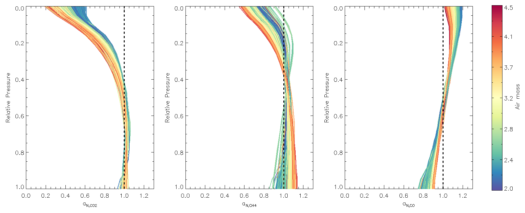
Figure 4 Normalized averaging kernel vectors a_N for $X_{{\mathrm{CO}}_{\mathrm{2}}}$, $X_{{\mathrm{CH}}_{\mathrm{4}}}$, and X_CO for all soundings passing our quality flag (Sect. 5.1), colored by air mass factor.

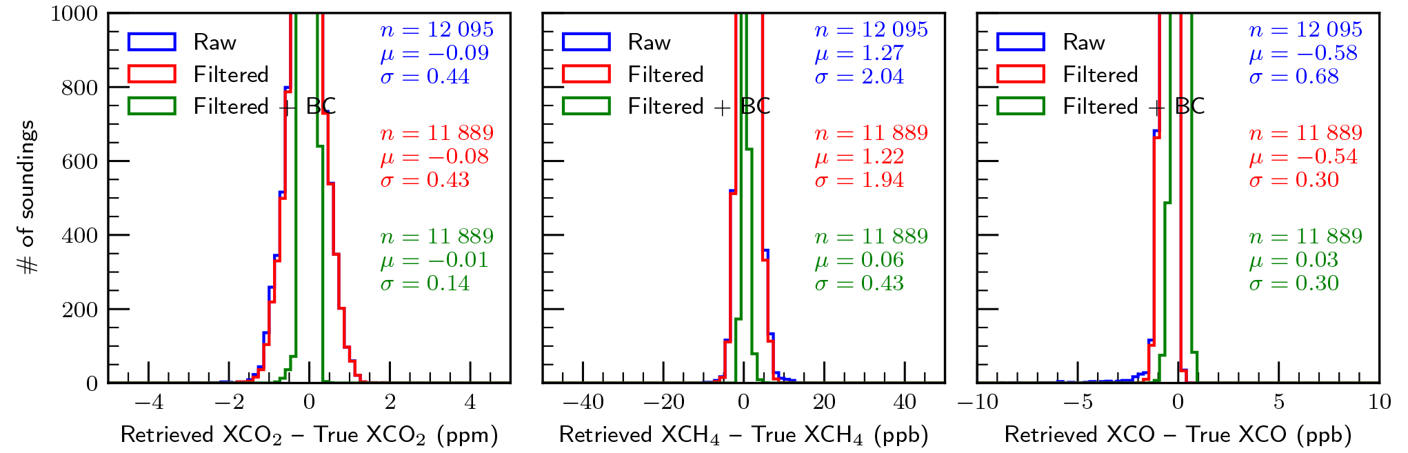
Figure 5 Baseline retrieval error results without clouds and aerosols (clear-sky) for three cases: unfiltered (raw), filtered, and filtered and bias corrected (BC). Statistics include the number of soundings n, the average error μ, and the standard deviation of the errors σ.

4.3.3 Averaging kernel correction

In order to properly compare the retrieved X_gas to the true value, the averaging kernel matrix from the retrieval is used to construct a gas profile u_gas,ak that is comparable to the retrieved profile in that it contains influence from both the true profile and the prior profile in the same proportions as the retrieved profile:

$$\begin{array}{}\text{(15)}& {\mathit{u}}_{\mathrm{gas},\mathrm{ak}}={\mathbf{A}}_{\mathrm{gas}}{\mathit{u}}_{\mathrm{gas},\mathrm{true}}+(\mathbf{I}-{\mathbf{A}}_{\mathrm{gas}}){\mathit{u}}_{\mathrm{gas},\mathrm{ap}},\end{array}$$

where A_gas is the averaging kernel matrix for a particular gas; u_gas,true is the true gas profile, which in this case is from the simulation scene input from step 2 in the simulation process; u_gas,ap is the prior gas profile; and I is the identity matrix. We then convert this to the column-integrated fraction as

$$\begin{array}{ll}\text{(16)}& {\displaystyle }{X}_{\mathrm{gas},\mathrm{ak}}& {\displaystyle }={\mathit{h}}^{\mathrm{T}}{\mathit{u}}_{\mathrm{gas},\mathrm{ak}}{\displaystyle }& {\displaystyle }=X_{\mathrm{gas},\mathrm{true}}+(\mathit{h}-{\mathit{a}}_{\mathrm{gas}}{)}^{\mathrm{T}}({\mathit{u}}_{\mathrm{gas},\mathrm{ap}}-{\mathit{u}}_{\mathrm{gas},\mathrm{true}}),\end{array}$$

where a_gas=h^TA_gas is the (un-normalized) averaging kernel vector for the gas in question, and the pressure weighting function h is defined by the pressure level intervals in the profile normalized by the surface pressure. The X_gas retrieval error is then given simply by

$$\begin{array}{}\text{(17)}& \mathrm{\Delta }{X}_{\mathrm{gas}}={\widehat{X}}_{\mathrm{gas}}-X_{\mathrm{gas},\mathrm{ak}},\end{array}$$

where ${\widehat{X}}_{\mathrm{gas}}$ is the retrieved gas-column-integrated fraction. The averaging kernel matrix A_gas, prior profile u_gas,ap, and pressure weighting function h are all obtained from the L2FP output at 20 levels and are then interpolated to the 72 levels of the true profile u_gas,true. Unless otherwise stated, this is how the errors are determined in the various retrieval experiments.

A brief discussion on this “AK correction” is warranted. The averaging kernel vector a_gas quantifies the response of the retrieved X_gas to changes in the true gas profile, which can be written as

$$\begin{array}{}\text{(18)}& {\mathit{a}}_{\mathrm{gas},j}={\displaystyle \frac{\partial X_{\mathrm{gas}}}{\partial {\mathit{u}}_{\mathrm{gas},\mathrm{true},j}}},j=\mathrm{1}\mathrm{\dots }n,\end{array}$$

where n is the number of vertical levels. This quantity is straightforward to derive from the full retrieval averaging kernel matrix A and several other quantities (see, e.g., Connor et al., 2008). It is common to normalize this quantity with respect to the pressure weighting function:

$$\begin{array}{}\text{(19)}& {\mathit{a}}_{N,\mathrm{gas},j}={\displaystyle \frac{{\mathit{a}}_{\mathrm{gas},j}}{{\mathit{h}}_j}}.\end{array}$$

This normalized averaging kernel vector can have values from below 0 to greater than 1. A value of unity means that a given change in the true gas profile causes a fully proportional change in the retrieved gas column fraction; i.e., there is no influence from the prior. For a perfect retrieval with perfect sensitivity, the values would all be unity.

Figure 4 shows the normalized averaging kernel vectors for $X_{{\mathrm{CO}}_{\mathrm{2}}}$, $X_{{\mathrm{CH}}_{\mathrm{4}}}$, and X_CO for our GeoCarb simulations, taken for all soundings that pass the post-retrieval quality flag in the baseline experiments (Sect. 5.1). From the figures it can be seen that the sensitivity to CO₂ and CH₄ is larger closer to the Earth's surface and is generally a function of air mass. This is as expected and optimal for the GeoCarb mission due sensitivity to sources and sinks at the surface. On the other hand, there is generally a slight increase in sensitivity to X_CO with altitude. These AKs are very similar to their up-looking counterparts from TCCON (e.g., Wunch et al., 2011a, Fig. 4)

Figure 6 Same as Fig. 5 but with clouds and aerosols (all-sky).

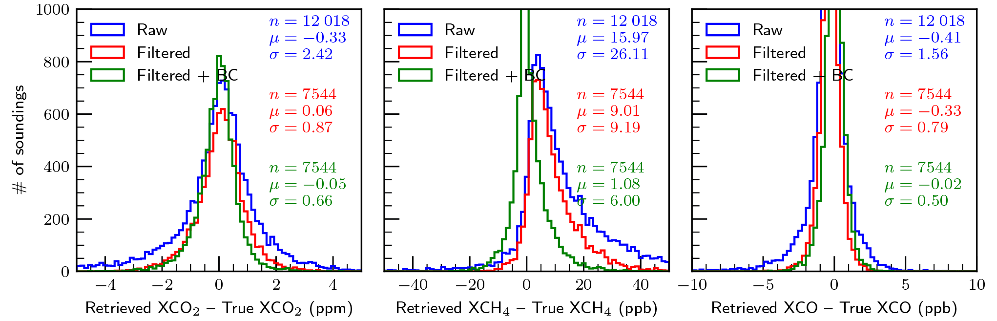
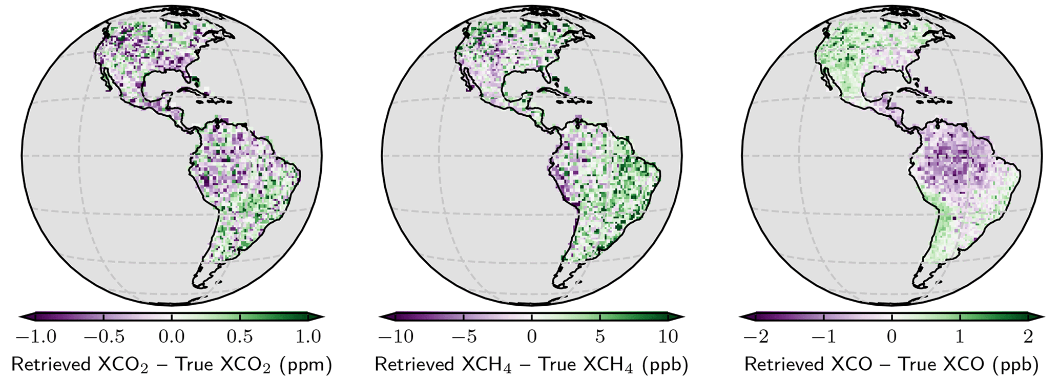
Figure 7 Maps of same results shown in Fig. 6 for the filtered and bias-corrected case.

5 Results

In this section, results are presented for each experiment in the order listed in Table 6. Though the GeoCarb mission requirements have no formal requirement on accuracy, we will take the multi-sounding precision requirements to similarly apply to accuracy. That is, we will typically evaluate the mean and standard deviation of the error for a given gas column fraction and require both to be less than the requirements given in Table 1.

There are two important details about the sounding selection process in the presentation:

• There will be a certain number of soundings that did not converge in the inversion process discussed in Sect. 3.1 which are not included in the analysis. These soundings did not converge, either due to too much aerosol and/or cloud and did not get filtered out in the pre-screening process or have other physical attributes that are not adequately represented in the forward model.

• The results presented are the intersection of the set of baseline results with the set of results of the particular experiment. This means that only soundings that converged in both cases are shown. As a result, the presentation of the baseline results will contain the highest number of soundings, and all other cases will contain as many as or fewer than the baseline results.

Results are shown for three cases: unfiltered (“Raw”), filtered (“Filtered”), and filtered and bias corrected (“Filtered + BC”). The statistics presented include the number of soundings n in the plot, the mean error μ, and the standard deviation of the errors σ.

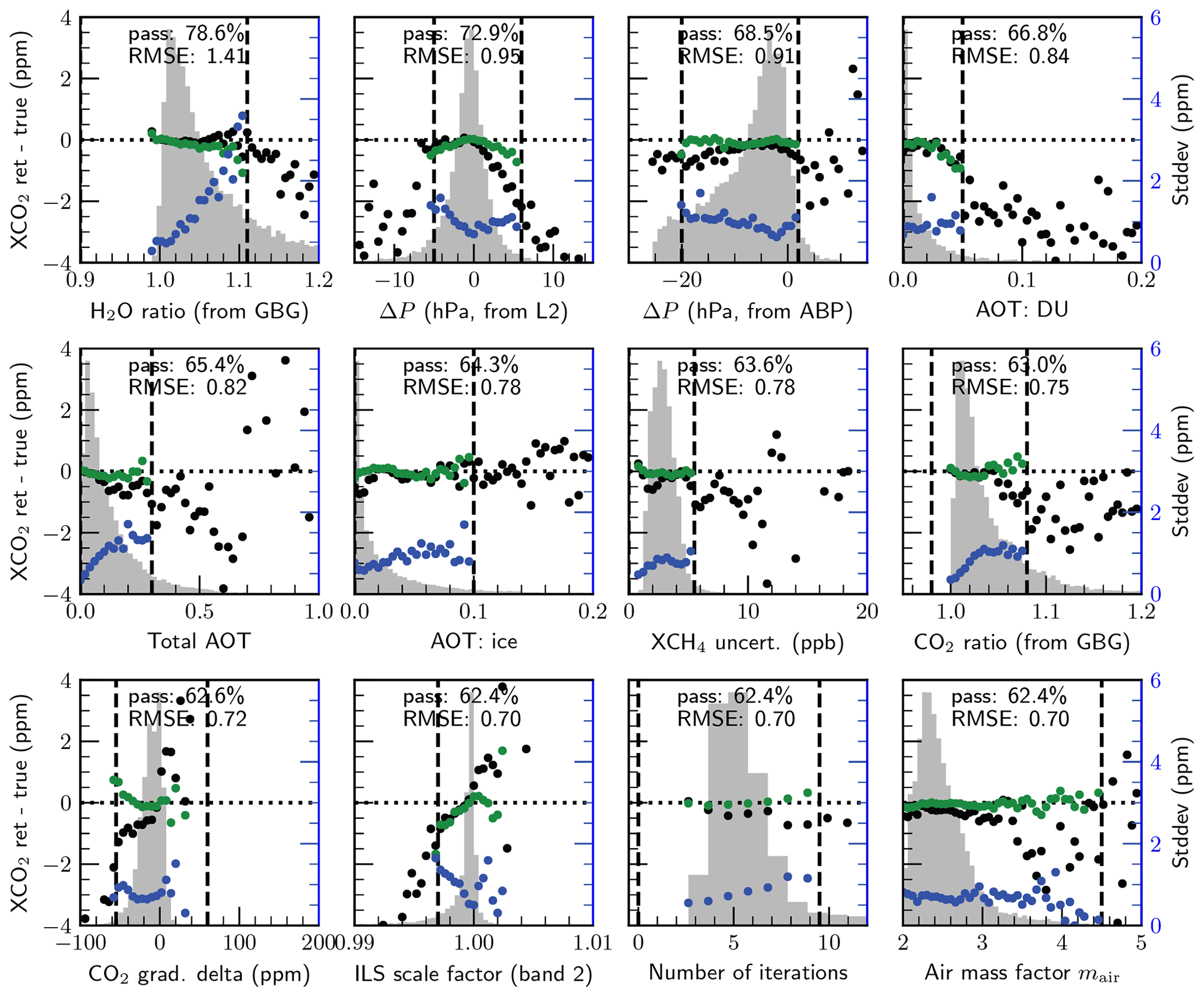
Figure 8 The top-12 most important filters in the post-processing filtering algorithm applied cumulatively and sorted by importance from left to right and then from top to bottom. Background histograms show the distribution of the filter variable values; the black dots show mean values of the difference between retrieved $X_{{\mathrm{CO}}_{\mathrm{2}}}$ and true $X_{{\mathrm{CO}}_{\mathrm{2}}}$ for each histogram bin (left axis), the blue dots show the standard deviation of the $X_{{\mathrm{CO}}_{\mathrm{2}}}$ differences for each histogram bin (right axis), and the green dots show the mean $X_{{\mathrm{CO}}_{\mathrm{2}}}$ differences for each bin after filtering and bias correction (left axis). The filter thresholds are shown as vertical dashed lines. The percentage of retrievals that pass the filter and RMSE of the results after the filter's application are also given for each variable.

5.1 Baseline

Figures 5 and 6 present histograms of retrieval errors for $X_{{\mathrm{CO}}_{\mathrm{2}}}$, $X_{{\mathrm{CH}}_{\mathrm{4}}}$, and X_CO for the baseline case, i.e., perfect knowledge of all variables investigated, for the special case with aerosols and clouds artificially removed (clear-sky) and for the case with aerosols and clouds included (all-sky), respectively. It is clear that the errors in the clear-sky case are significantly fewer compared to the all-sky case. This is as expected and is really a sanity check for the simulation system. The percentage of soundings making it through the filters in the clear-sky case (95.4 %) is significantly higher than in the all-sky case (68.1 %). This is consistent with what we have already discussed in Sect. 3.6 in that the filtering process is designed to remove retrievals that are not reliable due to the presence of aerosols and clouds.

Table 7 Baseline filters applied cumulatively along with the thresholds and the percentage of retrievals that pass the filter and, for each gas, the mean error, standard deviation of the error, and the RMSE of X_gas after the filter's application. (The units are ppm, ppb, and ppb for $X_{{\mathrm{CO}}_{\mathrm{2}}}$, $X_{{\mathrm{CH}}_{\mathrm{4}}}$, and X_CO.)

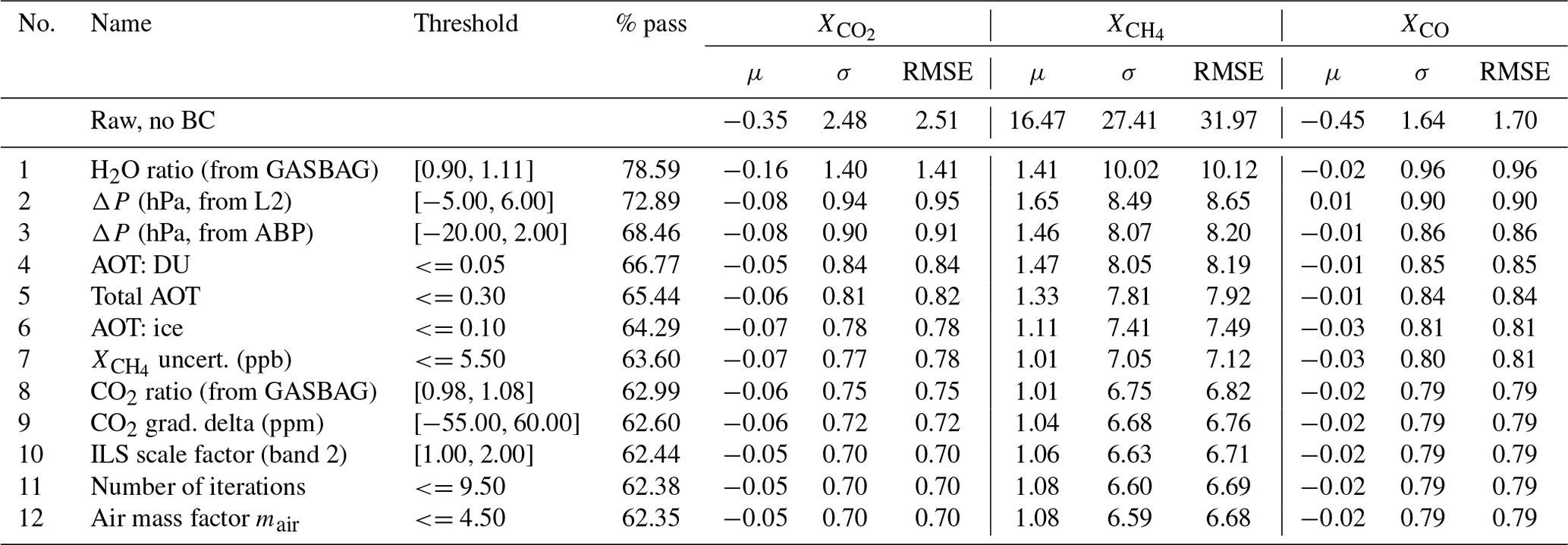
Table 8 Bias correction parameters. Aerosol types include the following: “wat”, liquid water particles; “ice”, ice crystals; “DU”, desert dust; “SS”, sea salt; “SU”, sulfate; and “OC”, organic carbon.

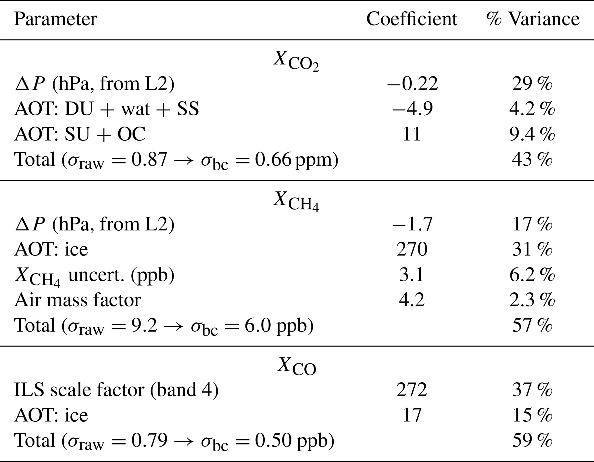
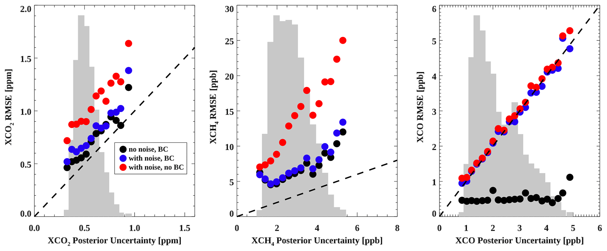
Figure 9 Baseline retrieval actual errors in target gas column fractions plotted vs. the posterior uncertainty. Shown are the noiseless errors with bias correction (black), with noise without bias correction (red), and with noise with bias correction (blue).

It is not surprising that the filtered and bias-corrected clear-sky retrievals meet the mission precision requirements listed in Table 1 (even the raw unfiltered results meet the requirements), but the all-sky filtered and bias-corrected results also meet the precision requirements with RMSEs of 0.66 ppm, 6.4 ppb, and 2.4 ppb for $X_{{\mathrm{CO}}_{\mathrm{2}}}$, $X_{{\mathrm{CH}}_{\mathrm{4}}}$, and X_CO, respectively. These are of course the results for the case of perfect knowledge of the variables investigated and with no random noise added. It is apparent from the plots that the retrievals of $X_{{\mathrm{CO}}_{\mathrm{2}}}$, and especially $X_{{\mathrm{CH}}_{\mathrm{4}}}$, are driven primarily by systematic errors, which is clearly not the case for X_CO. The large median bias in $X_{{\mathrm{CH}}_{\mathrm{4}}}$ of −6.59 ppb is curious and may be due to a significant bias in the $X_{{\mathrm{CH}}_{\mathrm{4}}}$ prior (mean bias ∼40 ppb). Any mean biases for these gas columns are largely removed by the bias correction.

Maps of the all-sky baseline results are shown in Fig. 7 for the filtered and bias-corrected case. Features include positive biases in $X_{{\mathrm{CO}}_{\mathrm{2}}}$ and X_CO at larger satellite zenith angles. Negative biases are apparent in $X_{{\mathrm{CH}}_{\mathrm{4}}}$ over high-altitude areas due to difficulty retrieving in these areas, although it is unclear why this is only apparent for methane. Finally, small negative biases in X_CO of order −1 ppb are prevalent over the Amazon, likely due to persistent cloud cover that either has not been pre-screened out or caught by the filtering.

Figure 10 Same as Fig. 6 but with synthetic Gaussian noise added.

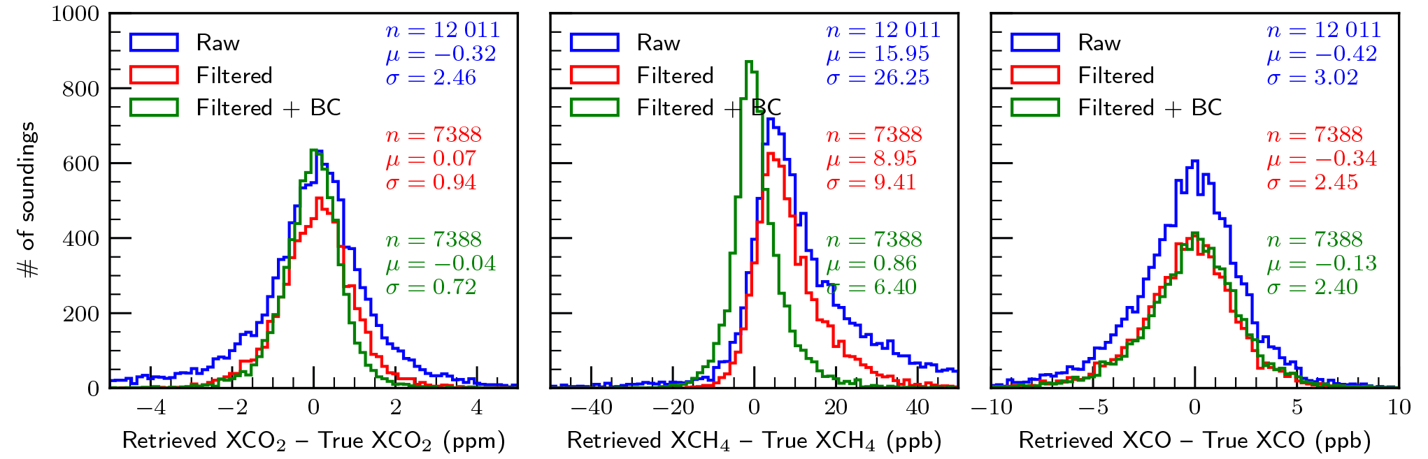
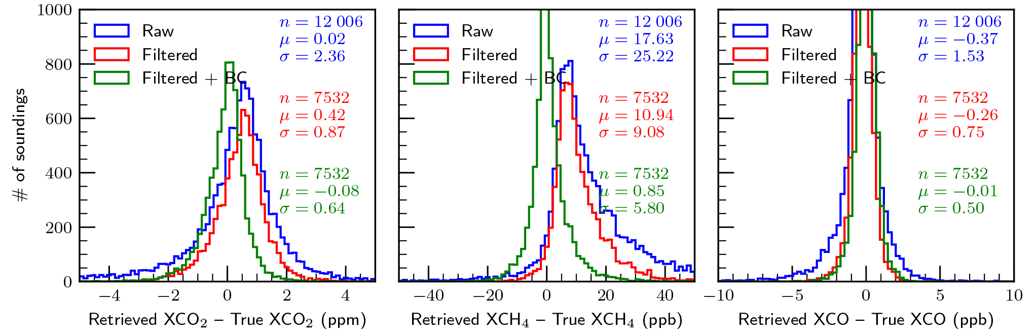
Figure 11 Same as Fig. 6 but for the case of imperfect knowledge of radiometric calibration for all bands.

Figure 12 Same as Fig. 6 but with imperfect knowledge of the ILS.

Figure 13 Same as Fig. 6 but with imperfect knowledge of polarization.

Figure 14 Same as Fig. 6 but with imperfect knowledge of the instrument pointing.

Figure 15 Same as Fig. 6 but with imperfect knowledge of meteorology.

Figure 16 Same as Fig. 6 but with imperfect knowledge of spectroscopy.

Figure 17 Same as Fig. 6 but for the kitchen sink experiment.

Figure 18 Same as Fig. 6 but for the kitchen sink with noise experiment.

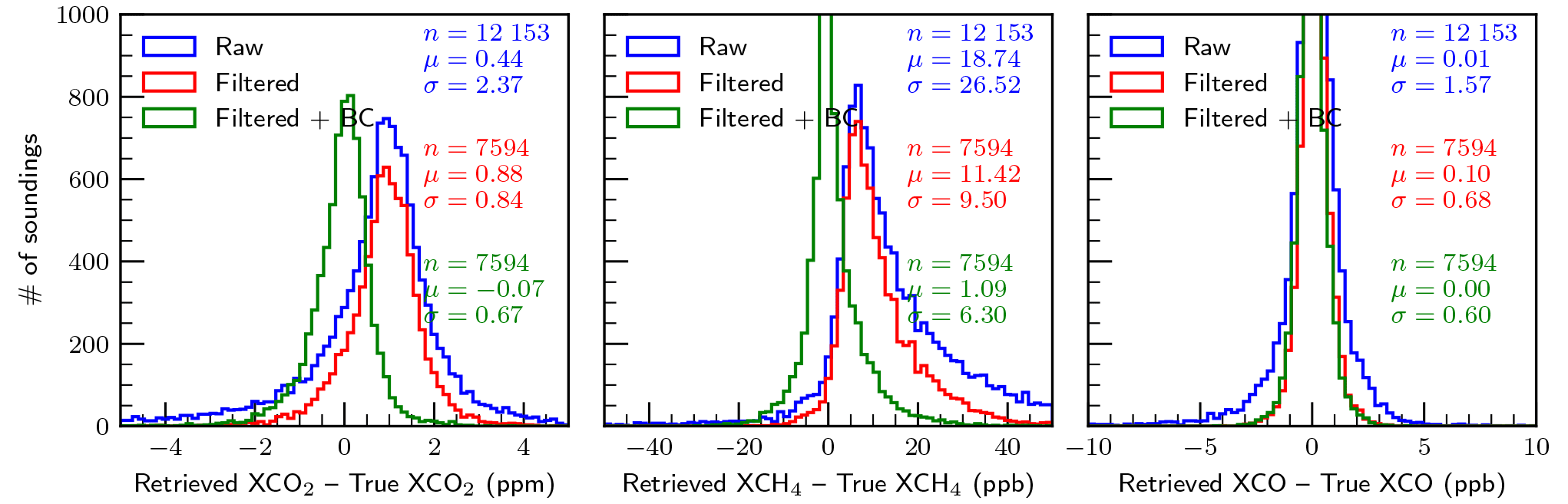
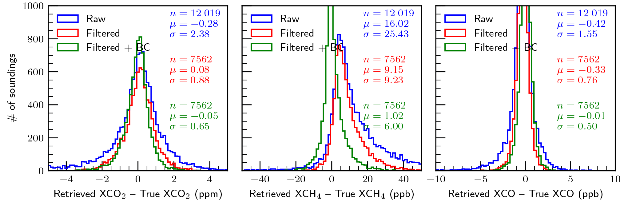
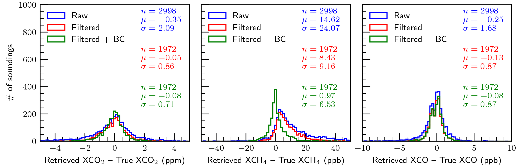
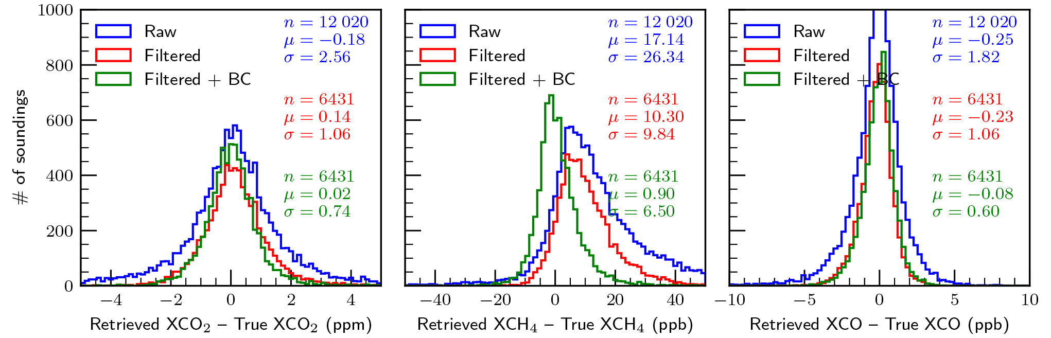
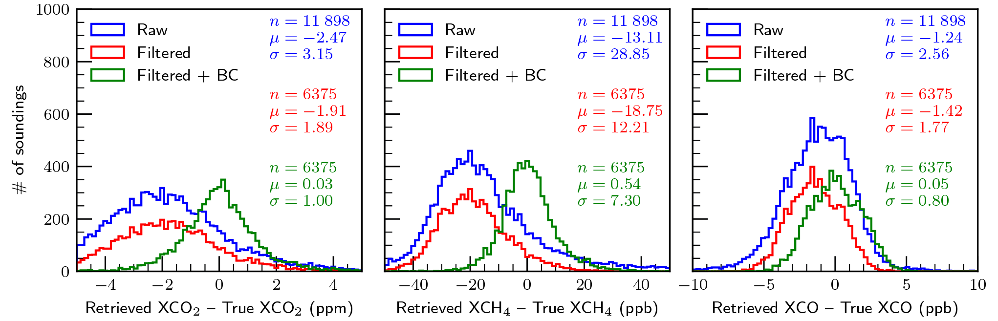
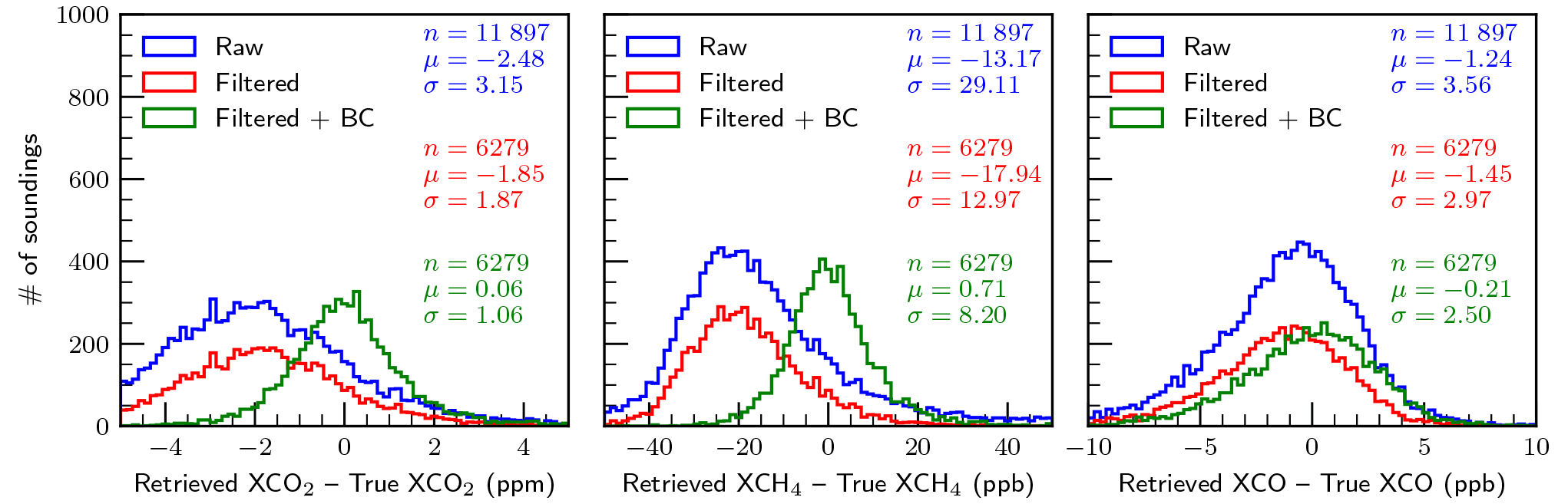
Table 9 Final error budget for each experiment, filtered and bias-corrected, including the total error and the component error (the error caused by the experiment's perturbation alone). N_proc is the number of soundings processed after pre-screening, N_conv is the number of soundings that converged, and N_good is the number of soundings that passed the filtering.

5.1.1 Quality filtering

The post-retrieval filtering approach is demonstrated in Fig. 8, which shows $X_{{\mathrm{CO}}_{\mathrm{2}}}$ vs. the filtering parameters with the simulation inputs as the truth proxy. The top-12 most important filters are shown sorted by importance from left to right and then from top to bottom. Table 7 summarizes the results for all three gases. It is apparent that just a few variables do the bulk of the filtering and that overall the filter variables are almost always associated with negative biases in $X_{{\mathrm{CO}}_{\mathrm{2}}}$ and positive biases in $X_{{\mathrm{CH}}_{\mathrm{4}}}$.

The variable with the largest filtering effect (∼21 % of the soundings filtered out) is the H₂O ratio from GASBAG which filters out scenes with too much cloud and aerosol contamination. The CO₂ ratio is also a filter variable that indicates cloud and aerosol contamination but has much less of an effect than the H₂O ratio. Another important filter variable is $\mathrm{\Delta }P=\widehat{P}-P_{\mathrm{true}}$, where $\widehat{P}$ is the retrieved surface pressure from either the L2FP retrieval or the ABP retrieval. The importance of this variable is most likely due to photon-path-length-related effects from aerosols and clouds and the retrieval adjusting ΔP to compensate. The retrieved aerosol optical thickness (AOT) is also an important filter variable, specifically for the larger aerosol types including dust (DU) and ice cloud (ice) and the total AOT for all aerosols and clouds. Large values of dust AOT are particularly associated with large negative biases in $X_{{\mathrm{CO}}_{\mathrm{2}}}$ due to the increased sensitivity to large particles in the CO₂ bands relative to that to smaller particles. In contrast, ice crystal particles become a more important filter for large $X_{{\mathrm{CH}}_{\mathrm{4}}}$ and X_CO biases (not shown) due to a larger sensitivity of the $X_{{\mathrm{CH}}_{\mathrm{4}}}$ band to ice crystals. The $X_{{\mathrm{CH}}_{\mathrm{4}}}$-retrieved uncertainty filters out retrievals with significant scatter, although any specific source of this scatter is unknown. The CO₂ vertical gradient delta is defined as the difference in retrieved $X_{{\mathrm{CO}}_{\mathrm{2}}}$ between the surface and the retrieval pressure level at 0.7 times the surface pressure minus the same quantity for the prior given by

$$\begin{array}{}\text{(20)}& \mathrm{co}\mathrm{2}\mathrm{\_}\mathrm{grad}\mathrm{\_}\mathrm{del}=\left[c\left(\mathrm{1}\right)-c\left(\mathrm{0.7}\right)\right]-\left[c_{\mathrm{a}}\left(\mathrm{1}\right)-c_{\mathrm{a}}\left(\mathrm{0.7}\right)\right],\end{array}$$

where c(x) and c_a(x) are the retrieved and a priori CO₂ dry air mole fraction, respectively, at relative pressure x. Sounding altitude is a filter variable which may normally be attributed to pointing errors, but since knowledge of the pointing in the baseline results is “perfect”, the altitude may be a proxy for difficulties in making retrievals at high altitudes, including errors in the prior surface pressure, broken clouds, and/or the presence of snow/ice. The band 2 ILS scaling filter most likely indicates the case where an effect is not accounted for in the forward model with the ILS scaling compensating for it. The filtering finishes off with the air mass factor m_air, which is influenced by both the solar and satellite zenith angles, where large angles result in an increase in scattering effects and associated larger RT errors.

It must be noted that new filters usually need to be rebuilt when changes are made to the retrieval system. These changes include changes made to the radiances (due to calibration changes), spectroscopy, prior inputs, and finally the forward model physics. In the past, for OCO-2/3, new filters have been produced with each release of the L2FP product (O'Dell et al., 2011, 2018), and it is planned that new filters will be rebuilt for each GeoCarb release. For the experiments in this paper, filters were built for the baseline, and it was determined that these filters were sufficient for the radiometric calibration, ILS, polarization, and pointing experiments, although it was determined that new filters were required for the baseline with noise, spectroscopy, meteorology, and kitchen sink experiments (a specific set of filters for each).

5.1.2 Bias correction

Table 8 shows the bias correction parameters for the three target gases for the baseline experiment. ΔP explains the most variability in $X_{{\mathrm{CO}}_{\mathrm{2}}}$, followed by the AOT from large aerosols (dust, liquid water cloud, and sea salt) as well as the fine-mode aerosol (sulfate + organic carbon). These variables are all important in the operational OCO-2 $X_{{\mathrm{CO}}_{\mathrm{2}}}$ bias correction (O'Dell et al., 2018), so their selection is not surprising. However, we see ΔP is also important for $X_{{\mathrm{CH}}_{\mathrm{4}}}$, but even more important is the retrieved ice cloud AOT, explaining 31 % of the variance in retrieved $X_{{\mathrm{CH}}_{\mathrm{4}}}$. And, even though X_CO is mostly dominated by random error, the bias correction still reduces the systematic error from 0.8 to 0.5 ppb.

5.1.3 Posterior uncertainty

The posterior estimate of uncertainty of X_gas for the baseline run (with aerosol/cloud and without noise added) is shown in Fig. 9. The posterior uncertainty for X_gas is given by

$$\begin{array}{}\text{(21)}& {\mathit{\sigma }}_{X_{\mathrm{gas}}}=\sqrt{{\mathit{h}}^{\mathrm{T}}{\widehat{\mathbf{S}}}_{\mathrm{gas}}\mathit{h}},\end{array}$$

where ${\widehat{\mathbf{S}}}_{\mathrm{gas}}$ is the portion of the posterior covariance matrix that is for either the CO₂, CH₄, or CO retrieved profiles. While these error estimates should generally be a combination of instrument noise and forward model errors, for simplicity our input error estimates only include instrument noise, smoothing error (related to the prior covariance), and interference errors with unrelated state vector elements. Our posterior error estimates do not include forward model errors (such as those due to spectroscopy, aerosol assumptions, surface characterization, and RT assumptions).

Figure 9 compares the RMSEs in the retrieved gas column fractions with the estimated posterior uncertainty described above. Shown are the baseline case including bias correction (black) and the baseline case with noise without (red) bias correction and with (blue) bias correction. The grey histograms indicate the distribution of the posterior uncertainties for each gas. The mean posterior (i.e., noise-driven) uncertainties are 0.53 ppm, 2.7 ppb, and 2.2 ppb for $X_{{\mathrm{CO}}_{\mathrm{2}}}$, $X_{{\mathrm{CH}}_{\mathrm{4}}}$, and X_CO, respectively. As expected, there is an underestimation of the error for both $X_{{\mathrm{CO}}_{\mathrm{2}}}$ and $X_{{\mathrm{CH}}_{\mathrm{4}}}$ due to the impact of systematic errors. This impact is largest for $X_{{\mathrm{CH}}_{\mathrm{4}}}$, indicating the importance of bias correction for that quantity. For X_CO (as well as SIF; see Somkuti et al., 2021), the uncertainties are more consistent with the actual errors, an indication that X_CO errors are driven less by systematic errors than $X_{{\mathrm{CO}}_{\mathrm{2}}}$ and $X_{{\mathrm{CH}}_{\mathrm{4}}}$, primarily due to less X_CO signal compared to the other gases. Relative to the noise-driven uncertainty, systematic errors in X_CO are almost negligible (less than 1 ppb).

5.2 Baseline with noise

The results when Gaussian noise is added to the baseline radiances are shown in Fig. 10. As already mentioned, a new filter was built specifically for this experiment. The results indicate that the precision requirements are met by the filtered and bias-corrected results with RMSEs of 0.72 ppm, 6.4 ppb, and 2.4 ppb for $X_{{\mathrm{CO}}_{\mathrm{2}}}$, $X_{{\mathrm{CH}}_{\mathrm{4}}}$, and X_CO, respectively. The filtering throughput of 7388 soundings (61 %) is, as expected, slightly less than that for the baseline (7544 soundings, 62 %). These relatively small impacts of the synthetic noise indicate that the retrievals of $X_{{\mathrm{CO}}_{\mathrm{2}}}$ and $X_{{\mathrm{CH}}_{\mathrm{4}}}$ are driven primarily by systematic errors, as we pointed out above. In contrast, the retrieval of X_CO is significantly affected by the addition of noise, supporting our previous observation that the X_CO retrieval is driven more by instrument noise. It is worth noting that in many applications the X_gas results will be averaged spatially and/or temporally, in which case it is expected that the random error will decrease proportionally to $\sqrt{n}$, where n is the number of soundings to be averaged.

5.3 Radiometric calibration

Results for the radiometric calibration perturbation experiment are shown in Fig. 11. In this experiment all channels were perturbed together by a scale factor of 1.05. From the figure it is apparent that even with the perturbation to the radiometric calibration, the filtered and bias-corrected X_gas results meet the precision requirements with RMSEs of 0.64 ppm, 5.8 ppb, and 0.5 ppb for $X_{{\mathrm{CO}}_{\mathrm{2}}}$, $X_{{\mathrm{CH}}_{\mathrm{4}}}$, and X_CO, respectively, and a filter throughput of 7532 soundings (62 %). These results are very similar to the baseline results, indicating that the retrieval is not particularly sensitive to an offset in the overall (multiplicative) radiometric calibration. As a test we performed this perturbation experiment with a 0.95 scale factor to make sure that the perturbation outcome is acceptably symmetric, which the results (not shown) indicate. The results for each band perturbed individually (not shown), a total of four additional tests, show only a small improvement when each is compared to the results, with all bands perturbed while compared to each other there is little noticeable differences between bands.

5.4 ILS

Results for the ILS perturbation experiment are shown in Fig. 12. The filtered and bias-corrected results all fall within the precision requirements with RMSEs of 0.67 ppm, 6.3 ppb, and 0.6 ppb for $X_{{\mathrm{CO}}_{\mathrm{2}}}$, $X_{{\mathrm{CH}}_{\mathrm{4}}}$, and X_CO, respectively, and a filter throughput of 7594 soundings (62 %). Again, perturbation symmetry was tested for this experiment with insignificant differences between perturbation directions. The results (with no bias correction) for each band perturbed individually (not shown) show a significantly larger bias in $X_{{\mathrm{CO}}_{\mathrm{2}}}$ results for bands 2 and 3 compared to bands 1 and 4. Clearly this is an indication of the sensitivity to CO₂ in these bands relative to the others. There are three state vector parameters that affect these results: to a small degree the dispersion scale and offset and, more importantly, the ILS scaling, all of which amount to a total of 12 parameters, three for each band. As mentioned before, we specifically removed the ILS scale factor from the state vector for this test and as it turns out (results not shown) including the ILS scale factor in the state vector fits for the perturbation error down to a negligible error for $X_{{\mathrm{CO}}_{\mathrm{2}}}$ and $X_{{\mathrm{CH}}_{\mathrm{4}}}$ and just to a small error compared to the baseline run for X_CO, most likely due to the smaller sensitivity to X_CO compared to the other gases. Regardless, it is still instructive to apply this perturbation without the ILS scaling in the state vector, to show that the bias correction can still largely correct for this error. It is worth noting that the simulations for these experiments do not include scene inhomogeneity, which can strongly perturb the ILS. This effect is described in Crowell et al. (2023).

5.5 Polarization

The results for the imperfect polarization experiment, wherein the retrievals assume the instrument is only sensitive to total intensity, when the simulations include a realistic polarization sensitivity, are shown in Fig. 13. The filtered and bias-corrected results all fall within the precision requirements with RMSEs of 0.65 ppm, 6.0 ppb, and 0.5 ppb for $X_{{\mathrm{CO}}_{\mathrm{2}}}$, $X_{{\mathrm{CH}}_{\mathrm{4}}}$, and X_CO, respectively, and a filter throughput of 7562 soundings (62 %). The per-band results (not shown) indicate the that there is no significant distinction per band. These findings are largely consistent with the earlier work in O2015 and indicate that a moderate knowledge of the instrument polarization response is sufficient to meet our requirements.

5.6 Pointing

The results for the experiment with a perturbation in pointing are shown in Fig. 14. In this case we were limited to the single day of 21 March 2016 without the 3 other days. We believe in this experiment that this reduced dataset will have little impact on the results. For this case, the filtered and bias-corrected results all fall within the precision requirements and are actually very close to the corresponding baseline results, with RMSEs of 0.67 ppm, 5.8 ppb, and 0.5 ppb for $X_{{\mathrm{CO}}_{\mathrm{2}}}$, $X_{{\mathrm{CH}}_{\mathrm{4}}}$, and X_CO, respectively. The throughput fraction of 65 % is marginally higher than that of the baseline (62 %), likely due to this particular day having slightly less cloud contamination.

5.7 Meteorology

The results for the meteorological perturbation experiment are shown in Fig. 15. The filtered and bias-corrected results meet the precision requirements with RMSEs of 0.74 ppm, 6.5 ppb, and 0.6 ppb for $X_{{\mathrm{CO}}_{\mathrm{2}}}$, $X_{{\mathrm{CH}}_{\mathrm{4}}}$, and X_CO, respectively. The errors are similar to the baseline, though with its own filter. This is at the cost of less filter throughput, with only 53 % soundings passing the quality filter versus 62 % for the baseline. Several parameters change significantly, in particular ΔP and co2_grad_del, which will affect the filtering. Finally, these filters were hand-tuned for simplicity, so some of the loss may simply be an imperfect filter.

5.8 Spectroscopy

The results for the spectroscopy perturbation experiment are shown in Fig. 16. The filtered and bias-corrected results all fall within the precision requirements, with RMSEs of 0.84 ppm, 7.5 ppb, and 0.6 ppb for $X_{{\mathrm{CO}}_{\mathrm{2}}}$, $X_{{\mathrm{CH}}_{\mathrm{4}}}$, and X_CO, respectively. As already mentioned, a new filter (not shown) was built for this experiment, but this was at the cost of significantly less filter throughput compared to the baseline with only 6290 soundings passing (52 %), similar to the meteorology perturbation experiment. Except for aerosols and clouds, error due to spectroscopy represents the largest single systematic error source we studied in this work. This is consistent with previous error analysis done for OCO-2 $X_{{\mathrm{CO}}_{\mathrm{2}}}$ retrievals (Connor et al., 2016; Hobbs et al., 2020).

5.9 Kitchen sink

The results for the kitchen sink experiment, which simultaneously includes all the individually discussed error sources above, are shown in Fig. 17. The errors for $X_{{\mathrm{CO}}_{\mathrm{2}}}$ meet the precision requirements for all three target gases, with RMSEs of 0.84 ppm, 7.5 ppb, and 0.6 ppb for $X_{{\mathrm{CO}}_{\mathrm{2}}}$, $X_{{\mathrm{CH}}_{\mathrm{4}}}$, and X_CO, respectively. In addition, the same experiment was done with Gaussian noise added to the radiances. All three target gas species still meet our mission requirements after filtering and bias correction. The results from $X_{{\mathrm{CO}}_{\mathrm{2}}}$ and $X_{{\mathrm{CH}}_{\mathrm{4}}}$ are similar to those from radiances without noise, while the largest effect of adding noise was for X_CO. The quadratic differences of these are another estimate of the pure-noise-driven error or precision of our measurements, which are roughly 0.3 ppm, 3.6 ppb, and 2.3 ppb for $X_{{\mathrm{CO}}_{\mathrm{2}}}$, $X_{{\mathrm{CH}}_{\mathrm{4}}}$, and X_CO, respectively. These values are roughly consistent with results from the baseline experiment with noise added. The fraction passing the quality filter, 53 % without noise and 52 % with noise, is significantly less than the baseline and is primarily driven by the spectroscopy and meteorological errors.

5.10 Error budget

Table 9 attempts to provide an approximate overall error budget for the target gases analyzed here. The errors are for filtered and bias-corrected results. The error for each experiment is listed including the total error for each X_gas (standard deviation σ given in the corresponding error histograms) and the component error, i.e., the error caused by the experiment's perturbation alone relative to the baseline. The component errors were calculated by assuming they are independent of the systematic errors in the baseline “with aerosols and clouds (a/c)” run, which thus add in quadrature. So, for component j,

$$\begin{array}{}\text{(22)}& X_{\mathrm{gas},j}=\sqrt{X_{\mathrm{gas},j}^{\mathrm{2}}-X_{\mathrm{a}/\mathrm{c}}^{\mathrm{2}}}.\end{array}$$

All experiments pass our precision and accuracy requirements given in Table 1. The component errors are estimates only and do not always add quadratically when combined. These errors are therefore only best guesses based upon the assumptions we have made. The dominant sources of systematic errors are, unsurprisingly, aerosols and clouds, meteorological errors, and spectroscopic errors. X_CO errors are dominated by random noise, while $X_{{\mathrm{CO}}_{\mathrm{2}}}$ and $X_{{\mathrm{CH}}_{\mathrm{4}}}$ are dominated by systematic errors. We can see that with perfect spectroscopy, typically 62 % of soundings pass the quality filters over land, but spectroscopic errors reduce this to ∼52 %. For $X_{{\mathrm{CO}}_{\mathrm{2}}}$, these results are surprisingly consistent with baseline errors and fractions seen by OCO-2 (O'Dell et al., 2018; Kiel et al., 2019).

6 Conclusions

The goal of this paper is to describe the GeoCarb L2FP algorithm and to present a study of the sensitivity of L2FP and the retrieved $X_{{\mathrm{CO}}_{\mathrm{2}}}$, $X_{{\mathrm{CH}}_{\mathrm{4}}}$, and X_CO to sources of uncertainty in several perturbation experiments using measurements simulated with the CSU L1B simulator. A description of the GeoCarb mission is given, and details of the L2FP algorithm are discussed. A description of the experimental dataset including the scan strategy is presented, the CSU simulator is described, and the individual experiments were described. The results were presented and discussed, and, finally, an error budget was presented in tabular form.

There are several key points that can be taken away from this study which are listed below:

• Retrievals errors of $X_{{\mathrm{CO}}_{\mathrm{2}}}$ and $X_{{\mathrm{CH}}_{\mathrm{4}}}$ are driven primarily by systematic errors.

• Retrievals errors of X_CO are primarily driven by random error, though these errors (∼ 2.5 ppb) are much smaller than the mission requirement of 12 ppb, suggesting GeoCarb will do better than expected with this important gas.

• The filtered and bias-corrected retrievals of $X_{{\mathrm{CO}}_{\mathrm{2}}}$, $X_{{\mathrm{CH}}_{\mathrm{4}}}$, and X_CO meet the mission precision requirements for all error sources, alone and in combination.

• Aerosols and spectroscopy form the majority of the systematic errors for all three gases.

• EOFs have not been included, and it is unclear what their effects will be, especially for the spectroscopy perturbation.

• The spectroscopic error experiments cause an additional ∼10 % of soundings to be filtered out. It is possible that by including EOFs in the retrieval, this effect could be mitigated.

• The calibration-related errors (radiometric gain, ILS, and polarization) do not account for a significant portion of the error in the results, but the calibration errors are not exhaustive. As mentioned before, this study does not account for other instrument effects such as smile, keystone, stray light, gain nonlinearity, and detector persistence. In addition, the effects of scene inhomogeneity are also not taken into account, and therefore ILS variation across the scene is ignored. These effects could end up being significant and will be treated in forthcoming papers.

• The filtering was trained for $X_{{\mathrm{CO}}_{\mathrm{2}}}$ for simplicity, although, given the larger errors for $X_{{\mathrm{CH}}_{\mathrm{4}}}$, it will most likely require more filtering and therefore its own filter. In contrast, X_CO will require less filtering. This will be addressed as the GeoCarb L2FP product is improved over time.

There are several next steps related to this study that are in progress or planned. As the instrument model develops, retrieval simulations will have to take into account the instrument effects, such as the effects of scene inhomogeneity and the other effects mentioned previously, that are ignored in this study. This will require modifications to the CSU simulator and the L2FP code. In addition, EOFs will be produced and their effects on the retrieval investigated. Finally, modifications to the filtering process to fine-tune the filtering for each gas separately are also planned. These next steps are ongoing or planned and will be addressed in subsequent papers.