Global evaluation of fast radiative transfer model coefficients for early meteorological satellite sensors

RTTOV (the Radiative Transfer for TOVS code, where TOVS is the TIROS Operational Vertical Sounder) coefficients are evaluated using a large, independent dataset of 25 000 atmospheric model profiles as a robust test of the diverse 83 training profiles typically used. The study is carried out for nine historical satellite instruments: the InfraRed Interferometer Spectrometer D (IRIS-D), Satellite Infrared Spectrometer B (SIRS-B), Medium Resolution Infrared Radiometer (MRIR) and High Resolution Infrared Radiometer (HRIR) for the infrared part of the spectrum, and the Microwave Sounding Unit (MSU), Special Sensor Microwave Imager (SSM/I), Special Sensor Microwave – Humidity (SSM/T-2), Scanning Multichannel Microwave Radiometer (SMMR) and Special Sensor Microwave Imager/Sounder (SSMI/S) for the microwave. Simulated channel brightness temperatures show similar statistics for both the independent and the 83-profile datasets, confirming that it is acceptable to validate the RTTOV coefficients with the same profiles used to generate the coefficients. Differences between the RTTOV and the line-by-line models are highest in water vapour channels, where mean values can reach up to 0.4 ± 0.2 K for the infrared and 0.04 ± 0.13 K for the microwave. Examination of the latitudinal dependence of the bias reveals different patterns of variability for similar channels on different instruments, such as the channel centred at 679 cm⁻¹ on both IRIS-D and SIRS-B, showing the importance of the specification of the instrumental spectral response functions (ISRFs). Maximum differences of up to several kelvin are associated with extremely non-typical profiles, such as those in polar or very hot regions.

1 Introduction

The fast radiative transfer model RTTOV (Radiative Transfer for TOVS, where TOVS is the TIROS Operational Vertical Sounder) (Saunders et al., 2018) is used as the observational operator that assimilates satellite measurements in multiple numerical weather prediction (NWP) models (i.e. Eyre et al., 2022), enables the retrieval of atmospheric or surface parameters (Merchant et al., 2019) or the simulation of satellite imagery from NWP models, and is also widely used across the world as a standalone model for scientific research applications (i.e. Chen and Bennartz, 2020). RTTOV is also being used more and more to train machine-learning-based approaches for simulating satellite observations (i.e. Scheck, 2021). The “fast” nature of RTTOV is attributed to the linear regression methods at its core, which combine pre-trained satellite gas absorption coefficients with various combinations of predictors for each atmospheric constituent in place of the full line-by-line atmospheric absorption calculation. The accuracy of the RTTOV transmittance parameterisation was first analysed by Saunders et al. (2007), who showed an overall agreement of within 0.05 K between different radiative transfer (RT) models and line-by-line (LBL) models, except for certain spectral regions. The evaluation was based on a subset of 49 atmospheric profiles selected from a large atmospheric profile dataset in the ECMWF ERA-40 database. This first study reported the spectral consistency of the LBL and RT models, but the low number of profiles used did not allow insights into the global distribution of the difference. The current validation of RTTOV coefficients of clear-sky simulations is based on the comparison between LBL simulations and the same results from RTTOV. The standard 83 training profiles used for coefficient generation are used in this validation.

The evaluation of RTTOV's performance presented in this study was carried out as one of the radiative transfer objectives for a project within the European Union's Copernicus Climate Change Service (https://www.copernicus.eu/en/copernicus-services/climate-change, last access: 7 February 2024) (C3S) entitled “C3S 311c: Support for climate reanalysis including satellite data rescue”. C3S is a program implemented by the European Centre for Medium-Range Weather Forecasts (ECMWF) that combines observations of the climate system with the latest science to develop authoritative, quality-assured information about the past, current and future states of the climate in Europe and worldwide. Recent advances in satellite data rescue for early satellite instruments are presented in Poli et al. (2017).

The first phase of the C3S 311c project comprised several concurrent data rescue studies that were carried out between 2019 and 2021, two of which were satellite based. The aims were to retrieve/rescue and reprocess historical infrared and microwave (MW) meteorological satellite observations from the 1970s and 1980s, primarily for inclusion in the ECMWF ERA6 reanalysis, the follow-on to ERA5 (Hersbach et al., 2020), which is due to enter production in 2024. In these reanalyses, RTTOV is employed to simulate all satellite radiance observations. An overview of all the objectives of RTTOV within the C3S 311c project is given in Vidot et al. (2021).

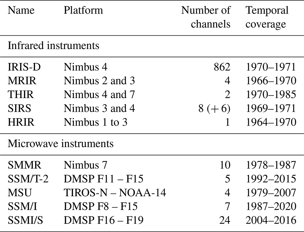
Different LBL models are used for infrared and microwave sensors. The validation of RTTOV coefficients is done for all instruments simulated by RTTOV, and the associated statistical data and figures can be found on the NWP Satellite Application Facility (NWPSAF) website (https://nwp-saf.eumetsat.int/site/software/rttov/download/coefficients/comparison-with-lbl-simulations/, last access: 7 February 2024). A further and more rigorous validation can be obtained by employing a larger independent profile dataset. The objective of this study is to provide further validation of the RTTOV coefficients by using a much larger independent dataset composed of 25 000 globally distributed profiles that were selected from 1 year of the IFS (Integrated Forecast System) NWP model and provided by NWPSAF. The validation is studied for the high-priority infrared instruments identified by the C3S 311c project, – the InfraRed Interferometer Spectrometer D (IRIS-D), Satellite Infrared Spectrometers A and B (SIRS-A and SIRS-B), Medium Resolution Infrared Radiometer (MRIR), and High Resolution Infrared Radiometer (HRIR) – and for the following microwave instruments: the Microwave Sounding Unit (MSU), Special Sensor Microwave Imager (SSM/I), Special Sensor Microwave – Humidity (SSM/T-2), Scanning Multichannel Microwave Radiometer (SMMR) and Special Sensor Microwave Imager/Sounder (SSMI/S); see Table 1.

Table 1 List of instruments studied in the C3S project and evaluated in the present study. Adapted from a GSICS newsletter (Vidot et al., 2021).

The 25 000 independent profiles and the 83 training profiles will be presented in Sect. 2. Section 3 presents a brief description of the high-priority infrared and microwave instruments identified by the project. Section 4 describes the LBL models used for the infrared and microwave instruments, which are the line-by-line radiative transfer model (LBLTRM) and the Advanced Microwave Sounding Unit Transmittance Model (AMSUTRAN), respectively, and the RTTOV versions used for the simulations. Validation results, in terms of the mean, standard deviation and maximum differences between the LBL and RTTOV simulations for both the 25 000 independent profiles and the training profiles will be presented in Sect. 5 for each satellite instrument. Analysis of the global position of each of the independent profiles and the spatial and latitudinal distributions of differences will also be shown for selected channels. The sixth section summarises the main results and draws conclusions from the previous sections.

2 Atmospheric profiles

The diverse profile training dataset contains 83 profiles for six molecules (water vapour (H₂O), ozone (O₃), carbon dioxide (CO₂), methane (CH₄), nitrous oxide (N₂O) and carbon oxide (CO)). One standard profile, mostly from the US76 standard atmosphere database (United States Committee on Extension to the Standard Atmosphere, 1976), is used for the other 22 molecules and chlorofluorocarbons (CFCs), though not every molecule is included for every instrument, depending on its spectral absorption coverage. The atmospheric profiles for the first six molecules were selected from a large database originally on 91 levels generated by the experimental suite (cycle 30R2) of the ECMWF forecasting system, as described in Chevallier et al. (2006). Profiles 81, 82 and 83 are the minimum, maximum and mean, respectively, of the initial database. We refer the reader to the RTTOV science and validation reports for a complete description of the training dataset, as listed in Saunders et al. (2017).

The larger independent set of atmospheric profiles used is described in Eresmaa and McNally (2014). Only values for water vapour, temperature and ozone profiles were used in the present evaluation. This dataset includes 25 000 profiles divided into five subsets, each with 5000 profiles. The profile is split into 137 levels from the surface to 0.01 hPa (training profiles present the same top of the model), which is the resolution currently used by the Integrated Forecasting System (IFS) developed at ECMWF. The dataset is selected from the short-range IFS (cycle 40r1) forecast over 1 year and is available from the NWPSAF website (https://www.nwpsaf.eu/site/software/atmospheric-profile-data/, last access: 7 February 2024). The five subsets of 5000 profiles represent the maximum variability of one of five different variables: temperature (t), specific humidity (q), ozone (O₃), cloud condensate (ccol) or precipitation (rcol).

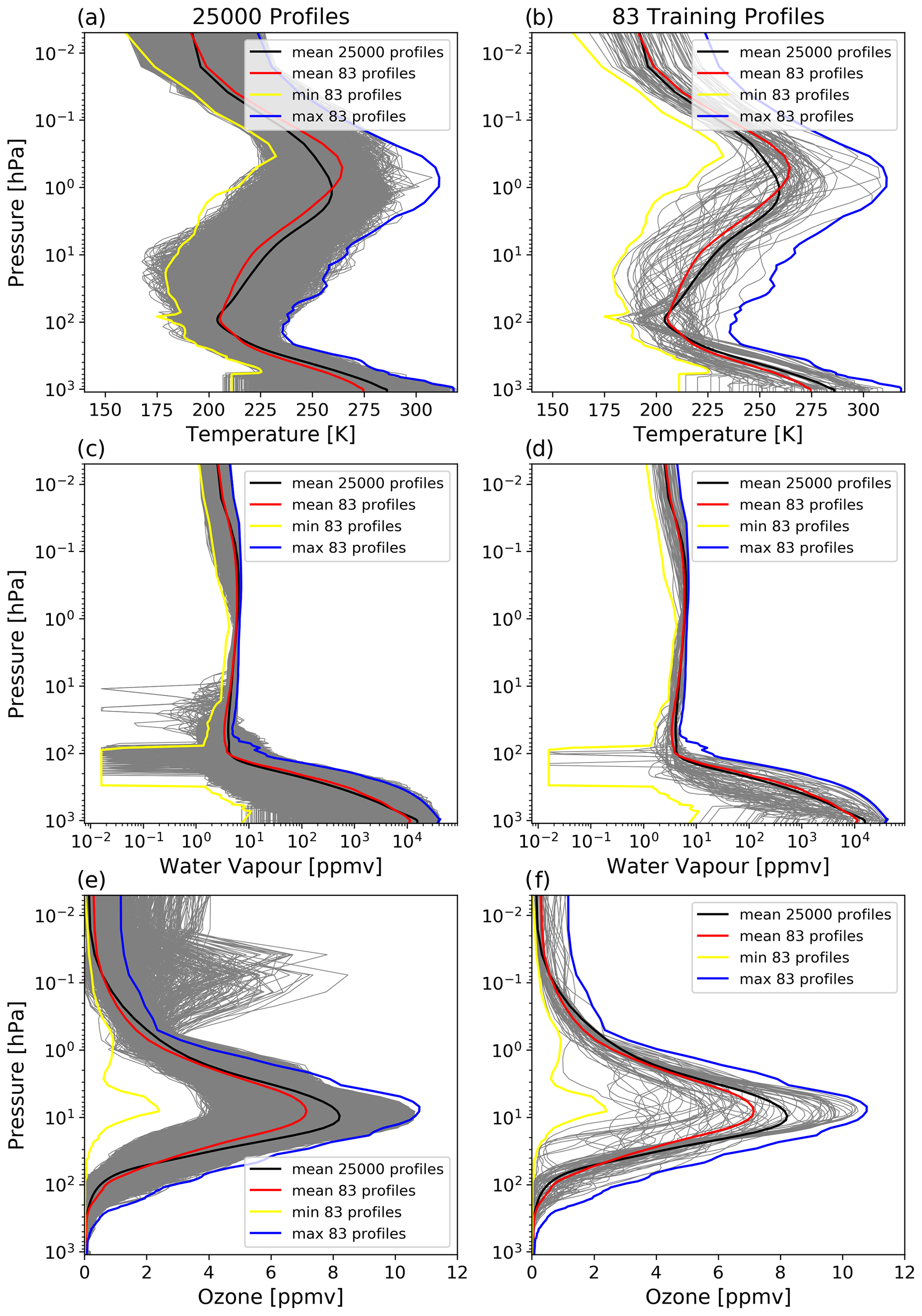
Figure 1 (a) 25 000 profiles of temperature (K) from the independent dataset, (b) 83 training profiles of temperature (K), (c) 25 0000 profiles of water vapour (ppmv) from the independent dataset, (d) water vapour profiles of 83 training profiles. (e, f) Ozone (ppmv) profiles from the independent dataset and training profiles, respectively. The mean profiles are shown for the 25 000 profiles (black lines) and the training profiles (red lines). The maximum (blue lines) and minimum (yellow lines) profiles for the 83 training profiles are also shown.

Figure 1 shows the temperature profiles (grey lines) for the 25 000 profiles and 83 training profiles (Fig. 1a and b, respectively). The mean profiles for the full 25 000 dataset (black lines) and for the 83 profiles (red lines) are also plotted on each panel. The vertical distributions of the maximum and minimum values are similar for the subsets and the training profiles; however, the mean stratopause height around 1 hPa is noticeably higher in the training set. This is probably due to the different vertical resolutions of the initial data from the ECMWF model, where the 137 levels of the larger dataset will better resolve the upper atmosphere than the 91 levels that comprise the training profiles. The maximum (minimum) temperature is 319.39 K (160.29 K) for the independent profiles and 318.25 K (159.61 K) for the training profiles.

Figure 1c and d also show the water vapour profiles of the 25 000 profile subsets and the training profiles, respectively. In the upper troposphere, the independent profiles generally have less water vapour than the training profiles do. The mean water vapour profiles (black and red lines) are similar. The minimum values of the two datasets are the same (0.016 ppmv), and the maximum value is 41 881 ppmv in the independent profiles and 42 868 ppmv in the training profiles.

The vertical distributions of ozone profiles are shown in Fig. 1e and f. The training profiles have less ozone in the stratosphere when compared to the independent dataset, which can be seen in the mean values. The mean ozone value around the peak level at 10 hPa is smaller in the training profiles relative to the independent profiles (7 ppmv versus 8 ppmv), and the ozone variability at this altitude is larger in the training profiles (Fig. 1f). The small values of ozone in the training profiles could be due to the presence of a profile located at the ozone hole. Ozone values vary between 0 and 10.65 ppmv in both datasets.

For all five subsets, the ozone distribution contains some profiles with a second peak of ozone above 1 hPa (only the ozone subset is shown in the Fig.  2), whereas this behaviour is not present in the training profiles. These profiles are located mainly in the polar regions. Figure 2a shows the spatial distribution of the profiles with a second peak taken from the ozone subset (the same behaviour is observed in the double-peak profiles from the other four subsets), and Fig. 2b shows their vertical distribution. The profiles were selected when the ozone content exceeded 3 ppmv above 0.9 hPa. In these profiles, the ozone concentrations are lower than average in the troposphere and mesosphere.

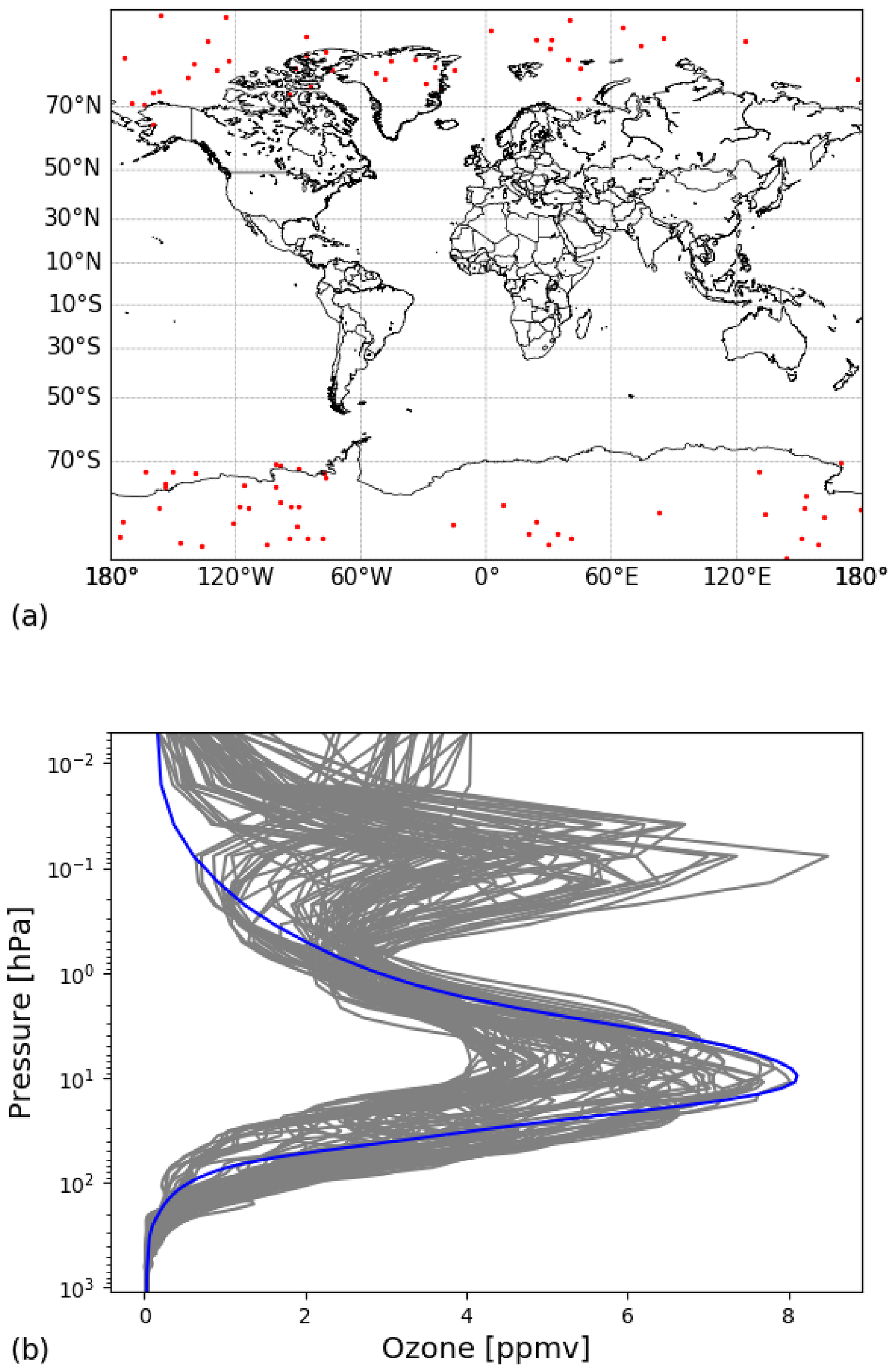
Figure 2 (a) Spatial and (b) vertical distributions of 87 ozone profiles from the ozone subset which present a double peak of ozone in the vertical distribution. These profiles have a second maximum of ozone quantity (higher than 3 ppmv) above 0.9 hPa. The mean ozone profile is represented by the blue line.

It is worth mentioning here that the RTTOV coefficients generated for the study were the ones with only water vapour and ozone as variable gases, which could be used for comparison with the dataset of 25 000 diverse atmospheric profiles.

3 Satellite instruments

3.1 Infrared instruments

3.1.1 IRIS-D

The InfraRed Interferometer Spectrometer (IRIS-D) was a hyperspectral IR sensor which had 862 channels (from 400.47 to 1597.71 cm⁻¹), spectral resolution 1.4 cm⁻¹, 94 km of spatial resolution at nadir and flew on Nimbus 4 (Hanel et al., 1971). This sensor presented channels in the CO₂ band (between 600 and 800 cm⁻¹), in the ozone band (near 1000 cm⁻¹), in the H₂O channels below 600 cm⁻¹ and above 1300 cm⁻¹, and it also had window channels.

3.1.2 SIRS-A and SIRS-B

The Satellite Infrared Spectrometer A (SIRS-A) was an infrared sensor which had eight channels (668.7 to 899 cm⁻¹) and flew on Nimbus 3 (Wark, 1970). Seven channels were in the CO₂ band (668.7 to 761 cm⁻¹) used for temperature sounding, and one window channel (899 cm⁻¹) was used for surface or cloud-top temperature retrieval. SIRS-B was an infrared sensor which had 14 channels (280 to 899 cm⁻¹), an increase of six relative to SIRS-A, and flew on Nimbus 4 (Hanel et al., 1972). SIRS-B's additional channels were in the H₂O rotational band (531 to 280 cm⁻¹), which was dedicated to water vapour profiling. The spatial resolution was 220 km at nadir for both sensors.

3.1.3 HRIR

The High Resolution Infrared Radiometer (HRIR), which had only one window channel (3.76 µm), essentially operated during nighttime only. It had a spatial resolution of 8 km and flew on Nimbus 1 and 2. The HRIR that few on Nimbus 3 was modified and had two channels: one visible channel (daytime) and one IR channel (nighttime).

3.1.4 MRIR

The other sensor is the Medium Resolution Infrared Radiometer (MRIR). This sensor had four channels (centred between 6.62 and 17.06 µm), flew on Nimbus 2 and 3, and presented spectral resolutions of 55 and 45 km. The channel centred at 17.06 µm had a very large bandwidth (between 5 and 30 µm).

3.2 Microwave instruments

3.2.1 MSU

The Microwave Sounding Unit (MSU) was a Dicke-type cross-track radiometer with a 110 km footprint (at nadir) that successfully flew on nine NOAA satellites between TIROS-N and NOAA-14 (not NOAA-13) (Spencer and Christy, 1990). It had four temperature-sounding double-passband channels in the 50–60 GHz oxygen region, each with a bandwidth of 200 MHz and a NEΔT (noise equivalent Δ temperature) of 0.3 K.

3.2.2 SSM/T-2

The Special Sensor Microwave – Humidity (SSM/T-2) was a total-power cross-track radiometer onboard four of the Defense Meteorological Satellite Program (DMSP) satellites between F11 to F15 (not F13) (Galin et al., 1993). It had five double-passband channels. The first two were centred at 91.6 and 150 GHz and were effectively window channels, and the remaining three sensed incrementally further away from and either side of the 183.31 GHz water vapour line. Footprint sizes ranged from 88 km for the 91.6 GHz channels to 48 km for all of the water vapour channels at nadir. All of them had an NEΔT of 0.6 K apart from the highest-peaking channel, channel 5 (183.31 ± 1.0 GHz), which had a value of 0.8 K.

3.2.3 SSM/I

The Special Sensor Microwave Imager (SSM/I) was a conical scanner that flew onboard seven of the DMSP satellites from F8–F15 (not F9) (Hollinger et al., 1990). It comprised seven double-passband channels with four frequencies, three of which had vertical and horizontal polarisation, and the remaining channel was vertically polarised and centred directly on the 22.235 GHz water vapour line. The other frequencies were in semi-window regions centred at 19.35, 37 and 85 GHz. Nadir footprint sizes varied between around 43 and 13 km depending on the channel. NEΔT values varied between 0.37 and 0.73 K.

3.2.4 SMMR

The Scanning Multichannel Microwave Radiometer (SMMR) was an early conical scanning instrument that flew on Nimbus 7 (Gloersen and Barath, 1977) and on a demonstrator mission on SeaSat, but the latter is not considered in this project. SMMR comprises 10 single-passband channels with five frequencies – one vertical polarisation channel and one horizontal polarisation channel for each frequency. The frequencies were all between 6.6 and 37 GHz and were primarily window channels, with some influence from the 22.235 GHz line. The footprint sizes varied from 148 km by 95 km at 6.6 GHz to 27 km by 18 km at 37 GHz. Values of NEΔT varied from 0.9 K for the lower-frequency channels to 1.5 K at the highest frequency measured.

3.2.5 SSMI/S

The Special Sensor Microwave Imager/Sounder (SSMI/S) is a 24-channel conical scanning instrument that has flown onboard all four DMSP satellites between F16 and F19 (Kunkee et al., 2008). With the most extensive coverage of the microwave instruments validated in this study (and the only one still flying at the time of writing), it is sensitive to a broad variety of atmospheric features and builds on the successes of the previous instruments as well as including new frequencies for high-level sounding. Five channels (12–16) are based on the lower-frequency surface-sensitive channels of SSM/I between 19.35–37 GHz, and five channels (9–11 and 17–18) are based on the higher-frequency channels of SSM/T-2 at 183.31 and 91.66 GHz, respectively. The first seven are temperature-sounding channels situated in the 50–60 GHz band. There are five very-high-resolution channels (19–23) centred at 60.79 GHz and another (channel 24) centred at 63.28 GHz which are sensitive to the upper levels of the atmosphere. Channel 8 at 150 GHz is a window channel. The footprint size varies from 74 km by 47 km for the 19 GHz channel to 15 km by 13 km for the 91 GHz channels. NEΔT varies from 0.2 K for the window channel to 1.23 K for channel 24. It should be noted that the Zeeman effect (the splitting of oxygen lines due to Earth's magnetic field), which may influence the high-peaking channels 19–22, is not modelled in the radiative transfer calculations.

4 Line-by-line models and RTTOV

4.1 Line-by-line radiative transfer model setup

4.1.1 Infrared instruments

The LBL simulation of the radiances at the top of the atmosphere (TOA) were performed with the Line-by-Line Radiative Transfer Model (LBLRTM) version 12.2 (Clough et al., 2005). LBLRTM v12.2 combines the Atmospheric and Environmental Research (AER) v3.2 molecular line database and the MT-CKD absorption continuum version 2.5.2. The AER v3.2 molecular database is based on the High-resolution Transmission molecular Absorption database (HITRAN) 2008 (Rothman et al., 2009), along with many improvements concerning the positions and intensities of some molecules and line-mixing effects (see a full description for each molecule at https://github.com/AER-RC/LBLRTM/wiki/What's-New, last access: 7 February 2024). The 101 (54) level profiles were used to simulate the hyperspectral (other) sensors. As previously mentioned, the independent profiles only contain temperature, water vapour and ozone information, profiles relating to the molecules CO₂, CH₄, N₂O and CO comprise the mean training profile set (profile 83), and there is one US76 standard profile for the other 22 molecules. The LBLRTM simulations were performed in one continuous band from 75 to 3325 cm⁻¹ with a spectral resolution of 0.001 cm⁻¹. The LBL simulations were then convolved by the instrument spectral response functions (ISRFs) of each sensor. To perform the convolution from radiances to instrument channels, the ISRFs used to generate the RTTOV coefficients were applied. The ISRFs are available at the NWPSAF website (https://www.nwpsaf.eu/site/software/rttov/download/coefficients/spectral-response-functions/, last access: 7 February 2024).

4.1.2 Microwave instruments

The line-by-line simulations for the microwave instruments were performed with AMSUTRAN (Turner et al., 2019), a line-by-line code dedicated to producing channel-averaged transmittances for microwave and sub-millimetre instruments which is maintained by the NWP SAF. The spectroscopy is based on Liebe (1989), with modifications made to key lines over time, such as the broadening parameters of the 22.235 and 183.31 GHz water vapour lines. Other major changes include updating all oxygen parameters with those provided by Tretyakov et al. (2005) and adding 35 of the strongest ozone lines below 300 GHz with parameters from HITRAN 2000 (Rothman et al., 2003).

The 25 000 profiles were interpolated to 54 levels before being ingested into the line-by-line code. The only gases included in the calculation are water vapour, oxygen, nitrogen (continuum only) and ozone, where the latter three are combined into a single mixed-gases transmittance profile. AMSUTRAN produces the instrument radiance by performing an “on-the-fly” calculation on a fine spectral grid over the bandwidth of each channel, the resolution of which is pre-determined based on the features of the spectrum, i.e. close proximity to a sharp oxygen line necessitates a higher resolution than a channel in a window region, for example. The channel resolutions for these five microwave instruments range between 0.005 and 50 MHz. The mean of the transmittance over the spectral grid gives one profile for each channel for both water vapour and the mixed gases. No spectral response function is applied, as it was found to be unavailable for these historical microwave instruments, so a top-hat/boxcar shape was assumed for each channel. This means that the choice of satellite for each series of instruments is immaterial, as they will all be the same.

The microwave simulations are less computationally intensive than the infrared ones, so it was possible to look at all six standard satellite zenith angles included in the RTTOV coefficients as well as the nominal nadir view. Of the five microwave instruments, only two, MSU and SSM/T-2, are cross-track scanners, so the full range of angles is presented for these two. The remaining three are conical scanners where the zenith angle is fixed; however, all six angles are still included in the coefficients. The microwave surface emissivity for all simulations is set to 1. Radiance and brightness temperature are calculated using a linear-in-tau approximation with the transmittance profile; see Berk et al. (1998). The same approximation was applied to the infrared.

4.2 RTTOV radiative transfer simulations

The RTTOV simulations were processed with the same profiles used for the LBL simulations, and they are all clear sky in line with the line-by-line models, which do not include any treatment of cloud or ice. Independent profiles were interpolated from the original 137 model levels to either 101 or 54 pressure levels, depending on the instrument. For hyperspectral instruments, 101 levels are required, as the full vertical stratification of the atmosphere is resolved, but 54 levels are sufficient for all other narrowband instruments (SIRS, MRIR, HRIR, MSU, SSM/I, SSM/T-2, SMMR, SSMI/S). For the infrared instruments, the version 7 predictor RTTOV coefficients (with 101 levels for IRIS-D and 54 levels for other instruments) were used because there is no variation in the carbon dioxide (CO₂) profile with these. Version 7 predictors were introduced at the release of RTTOV-7 and are a development of those used in RTIASI. There are 10 predictors specified for the mixed gases (e.g. O₂ and N₂), 15 for water vapour and 11 for ozone, and they are functions of satellite zenith angle, temperature, water vapour and ozone mixing ratio; see Saunders et al. (2002, Table 1) for full details and Saunders et al. (2018). As with the LBLRTM simulations, the CO₂ profile used in the RTTOV simulations was the mean training profile (profile number 83). The CO₂ value in profile 83 is around 400 ppmv, as described in Saunders et al. (2017). The infrared simulations were performed only at nadir viewing geometry. The RTTOV setup for the microwave instruments was the same as for the infrared instruments except for the satellite angle. For the microwave simulations, the standard six satellite zenith angles (SZAs) that vary between 0.0 to 63.6^∘ were used, which equates to secant values of 1.0, 1.25, 1.5, 1.75, 2.0 and 2.25. All microwave RTTOV simulations use version 7 predictors, and 54 (as opposed to 101) levels are sufficiently accurate for these instruments, as demonstrated by Saunders et al. (2013). The mean training profile for ozone is included in the mixed gases calculation, in the same manner as CO₂ in the infrared simulations, and hence ozone is not treated as a variable gas because its effects are very small in the microwave. All calculations are performed using an emissivity value of 1, which is limited by the line-by-line models that simulate strictly upwelling radiation and do not calculate the reflectance.

5 Independent profile dataset versus the training profile dataset

The evaluation was performed separately for each subset of 5000 profiles. However, the statistics were almost the same for each subset and for the ensemble of 25 000 profiles. For this reason, only the statistics for the 25 000 profiles (together) are shown. Note that the maximum difference can be either positive or negative, so we retain the sign of RTTOV-LBL rather than just reporting the absolute difference between them.

5.1 Statistical evaluation

5.1.1 IRIS-D

Figure 3​​​​​​​ shows the differences in the (a) average (AVG), (b) standard deviation (SD) and (c) maximum values (MAX) in the TOA brightness temperature (BT) simulations between RTTOV and LBLRTM for all IRIS-D channels. Overall, the mean differences between the independent profiles (blue lines) and the training profiles (red lines) are very similar and vary between −0.238 and 0.247 K. The differences between the two datasets are more evident in the CO₂ band (between 600 and 800 cm⁻¹) and in the ozone band (near 1000 cm⁻¹). Similar behaviour is found for the standard deviation of differences, which varies between 0.006 to 0.235 K. The highest standard deviation, and mean differences between datasets, is seen in the H₂O channels below 600 and above 1300 cm⁻¹. The variability of water vapour profiles in the independent profiles is greater than that in the training profiles, which could explain why they are higher. Conversely, the variability of the ozone profiles from the training profiles is higher in the ozone peak, which could explain the higher values of the standard deviation of mean differences in the ozone band. The statistics from the independent profiles have higher maximum values than the ones from the training profiles (up to 6 K in some channels, but mostly below 2 K, against 0.5 K in the training profiles), which is to be expected because they have more variability. The standard deviation of the differences presents a small value when compared against the instrument noise. The instrument noise is near 0.5 K between 600 and 1200 cm⁻¹, decreases from 4 to 0.5 K between 400 and 600 cm⁻¹, and increases from 0.5 up to 3.5 K above 1200 cm⁻¹.

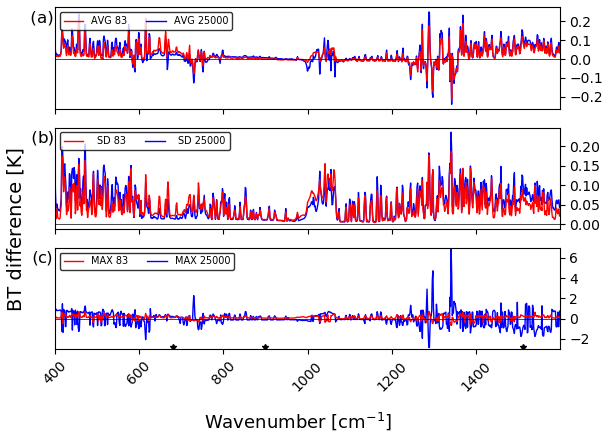
Figure 3 Difference between RTTOV and LBLRTM in brightness temperature (K) for IRIS-D in terms of (a) the mean differences, (b) the standard deviation of differences and (c) the maximum differences. Blue lines represent the independent profiles and red lines are the training profiles. The three stars represent the three IRIS-D channels analysed in the spatial evaluation.

5.1.2 SIRS-A and SIRS-B

Figure 4 shows the differences between RTTOV and LBLRTM in the (a) average (AVG), (b) standard deviation (SD) and (c) maximum (MAX) values in the TOA brightness temperature (BT) simulations for each channel for SIRS-B. For SIRS-B, statistics for the independent profiles and the training profiles have similar values. The mean differences for the training profiles (red bars) are only larger than those for the independent profiles (blue bars) in the channels centred at 14.95 and 22.91 µm; for all other channels, the reverse is found. The statistics for the training dataset are very good for channels below 15 µm as compared with the independent dataset, but, overall, the mean differences are between −0.05 and 0.2 K for all channels and for both datasets. The standard deviations are slightly larger in the independent profiles, but the two datasets have similar values and the standard deviation increases with wavelength for both datasets. As for the IRIS-D channels, the maximum values for SIRS-B are higher for the independent profiles, with values of up to 3.5 K against 0.5 K for the training dataset.

Figure 4 Same as Fig. 3 but for SIRS-B. The channels are represented by bars.

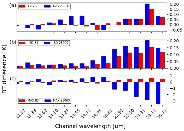
The first eight SIRS-B channels show statistics similar to the SIRS-A channels (figures not shown). For SIRS-A, the mean differences for the training profiles are only larger than those for the independent profiles in the channels centred at 14 and 14.95 µm; for all other channels, the reverse is found. For SIRS-A, the statistics for the training dataset are very good for channels below 14.94 µm as compared with the independent dataset, but, overall, the mean differences are between −0.05 and 0.1 K for all channels and for both datasets. For SIRS-A, the standard deviations are slightly larger in the independent profiles, but the two datasets have similar values and the standard deviation increases with wavelength for both datasets, although this is more evident in the independent profiles. As for the IRIS-D channels, the maximum values for SIRS-A are higher for the independent profiles, with values of up to 1 K against 0.2 K for the training dataset. These statistics of SIRS-A were also compared against the instrument noise. The 14 µm channel presents the highest value (0.7 K); in the other channels, the noise varies between 0.1 and 0.25 K, which are higher than the standard deviation of the differences (figure not shown).

5.1.3 HRIR and MRIR

Two other sensors were also analysed, HRIR and MRIR. The statistics of HRIR are very similar for both profile datasets (figure not shown). The statistics of MRIR are similar to those of SIRS and IRIS-D except in the channel centred at 17.06 µm, which presents the highest mean differences, standard deviation and maximum value (figure not shown). The main cause of this is probably the fact that this channel has a very large bandwidth (between 5 and 30 µm).

5.1.4 MSU

Temperature channels tend to perform well in RTTOV compared with the underlying line-by-line model, and this instrument is no exception (Fig. 5). In general, the differences between the two profile datasets are small, with slight decreases in the mean and standard deviation but an increase in the maximum value when using the larger dataset – all of which would be expected. The maximum difference in any channel is below 0.15 K.

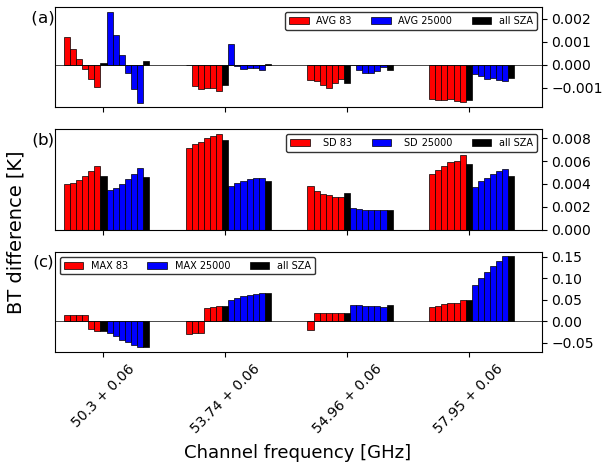
Figure 5 Differences in simulated brightness temperature (K) between RTTOV and AMSUTRAN for MSU channels in terms of (a) the mean (over all profiles), (b) the standard deviation, and, (c) the maximum difference. Blue bars represent the 25 000 profiles and red bars are the training profiles. Each statistic is split by SZA, with the nadir on the left and then the five subsequent SZA values up to 63^∘. The total statistics for all six SZAs are then shown in the following black bar for each of the two profile datasets.

The variation with satellite zenith angle varies depending on the channel, but the pattern of variation is similar for the two datasets. Channel 1, centred at 50.3 GHz, is more like a window channel than the other three and shows more of a dependency on SZA in general. Mean biases reduce and then become negative with increasing angle, giving an overall six-angle mean of near zero. Standard deviations increase slightly and so does the value of the maximum difference, with bigger values seen in the larger dataset, up to 0.5 K. The other three channels show relatively little angular dependence of the mean, a slight increase (or decrease in the case of channel 3) in the standard deviation, and little dependence of the maximum difference (apart from channel 4 in the larger dataset, where values increase with satellite zenith angle up to 0.15 K). Particularly in terms of the standard deviations, there is relatively little difference in statistics when using the nadir view only or all six satellite zenith angles.

5.1.5 SSM/T-2

For SSM/T-2, there is an approximate 10-fold increase in all difference statistics in comparison to MSU, which is to be expected, as water vapour is more difficult to predict than dry air due to its increased variability (Fig. 6). The pattern of mean statistics looks quite similar for both datasets. As with MSU, the maximum differences increase in the 25 000-profile set; however, the standard deviation increases instead of decreasing. As SSM/T-2 is a humidity-sensitive instrument, this is likely due to the broader range of water vapour profiles in a far larger dataset relative to the possible dry air profiles. Channel 3, which is the channel closest to the centre of the 183.31 GHz line, shows the largest increases in standard deviation and maximum difference, with the maximum changing from 0.2 to nearly −2 K.

Figure 6 Same as Fig. 5 but for SSM/T-2.

There is a similar variation of satellite zenith angle dependency in the mean bias of all channels; however, the standard deviation of the bias is relatively independent of angle. The nadir and the total angular mean are very close in value, indicating that one or the other could be used in bias correction schemes. Maximum differences become larger (in absolute value) with increasing zenith angle, almost doubling for most channels and profile sets.

5.1.6 SSM/I

There are similarities in the difference patterns to SSM/T-2 (not shown), as they are both window/water vapour sensing instruments and there are slightly larger difference statistics in the 25 000-profile dataset for all channels; however, the magnitudes for SSM/I are about 10-fold less than those for SSM/T-2, as they are at lower frequencies. Channel 3 at 22.235 GHz shows some similarities to the 183.31 GHz channels on SSM/T-2; however, the mean differences in the 25 000-profile dataset are larger in the 85.5 GHz channels. The maximum difference is −0.3 K in channel 3. When all six zenith angles are included, mean differences reduce quite significantly for both profile datasets; however, standard deviations increase. The maximum difference increases to −0.6 K in channel 3, though the other channels only reduce slightly.

5.1.7 SMMR

SMMR shares similarities with equivalent low-frequency channels on SSM/I, and the patterns are the same, with all of the statistics for the 25 000-profile dataset increased with respect to the training dataset (not shown). Channels 7 and 8 at 21 GHz show the largest differences as they are in close proximity with the 22.235 GHz water vapour line, with a maximum bias of −0.12 K but a mean value of just above 0.003 K. When all six satellite zenith angles are included, the mean differences significantly reduce, whereas standard deviations and maximum biases increase for both profile datasets, with a maximum bias of −0.27 K in channels 7 and 8. Brightness temperature differences are generally low as this is quite a flat part of the spectrum.

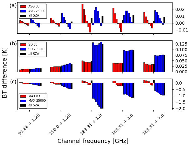
5.1.8 SSMI/S

SSMI/S has a conical viewing geometry with a fixed zenith angle of 53.1^∘, so the full range of SZAs calculated for the standard RTTOV coefficients will never be used. To test the accuracy of the validation statistics, which are an average of all six SZAs, Fig. 7 shows these values alongside just the fourth SZA, which is equal to a secant of 1.75 and an angle of about 55^∘, so it is very similar to SSMI/S. The biases are remarkably similar in most cases, indicating that the average of all SZA biases can be used to accurately represent the true viewing geometry biases if needed. As many of the channels are the same as or similar to channels in the previous instruments discussed, there are no big surprises in terms of behaviour. Water vapour channels 9–11 around 183.31 GHz show the biggest differences between RTTOV and AMSUTRAN and between the training profile set and the 25 000 profile set, as expected based on the corresponding channels on SSM/T-2. The higher-peaking channels 21–24 around 60 GHz show only slightly bigger differences than the lower temperature-sounding channels 1–7 between 50–60 GHz. These follow the same pattern as the MSU temperature-sounding channels but with lower standard deviations for the 25 000-profile dataset than the training profiles.

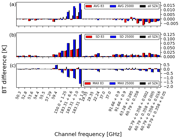
Figure 7 As Fig. 6 but for SSMI/S. Only the fourth SZA, secant = 1.75, is shown in the red/blue bars.

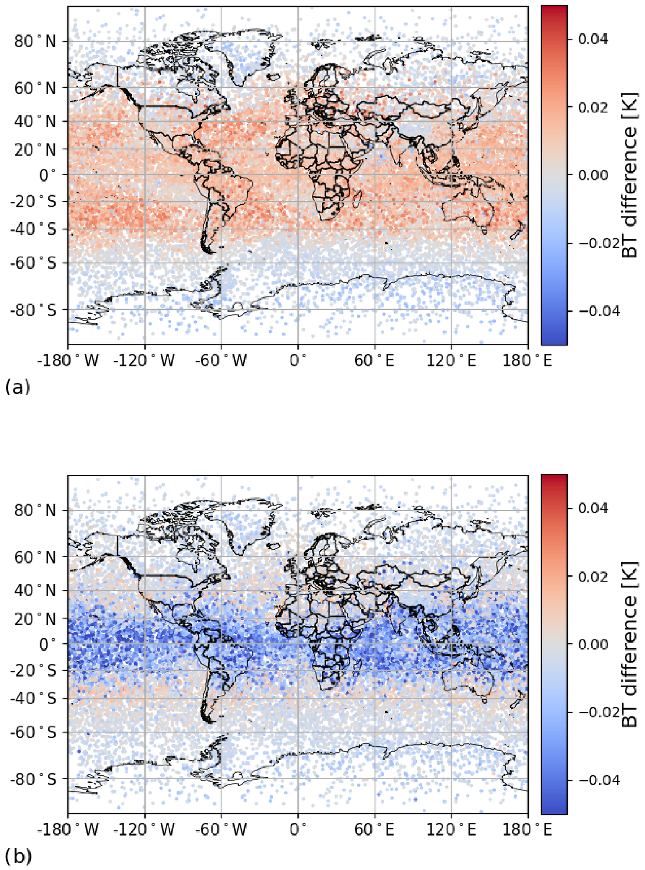
Figure 8 Spatial distribution of RTTOV minus LBLRTM for (a) channel 899.66 cm⁻¹ from IRIS-D and (b) channel 899.0 cm⁻¹ from SIRS-B. Each point represents one of the 25 000 profiles.

5.2 Spatial variation of bias from the independent dataset

When forming the statistics shown in the previous section, details are lost in the averaging process that are revealed with a spatial view of the biases over the entire globe, so the spatial variability for each profile in the independent dataset was also evaluated.

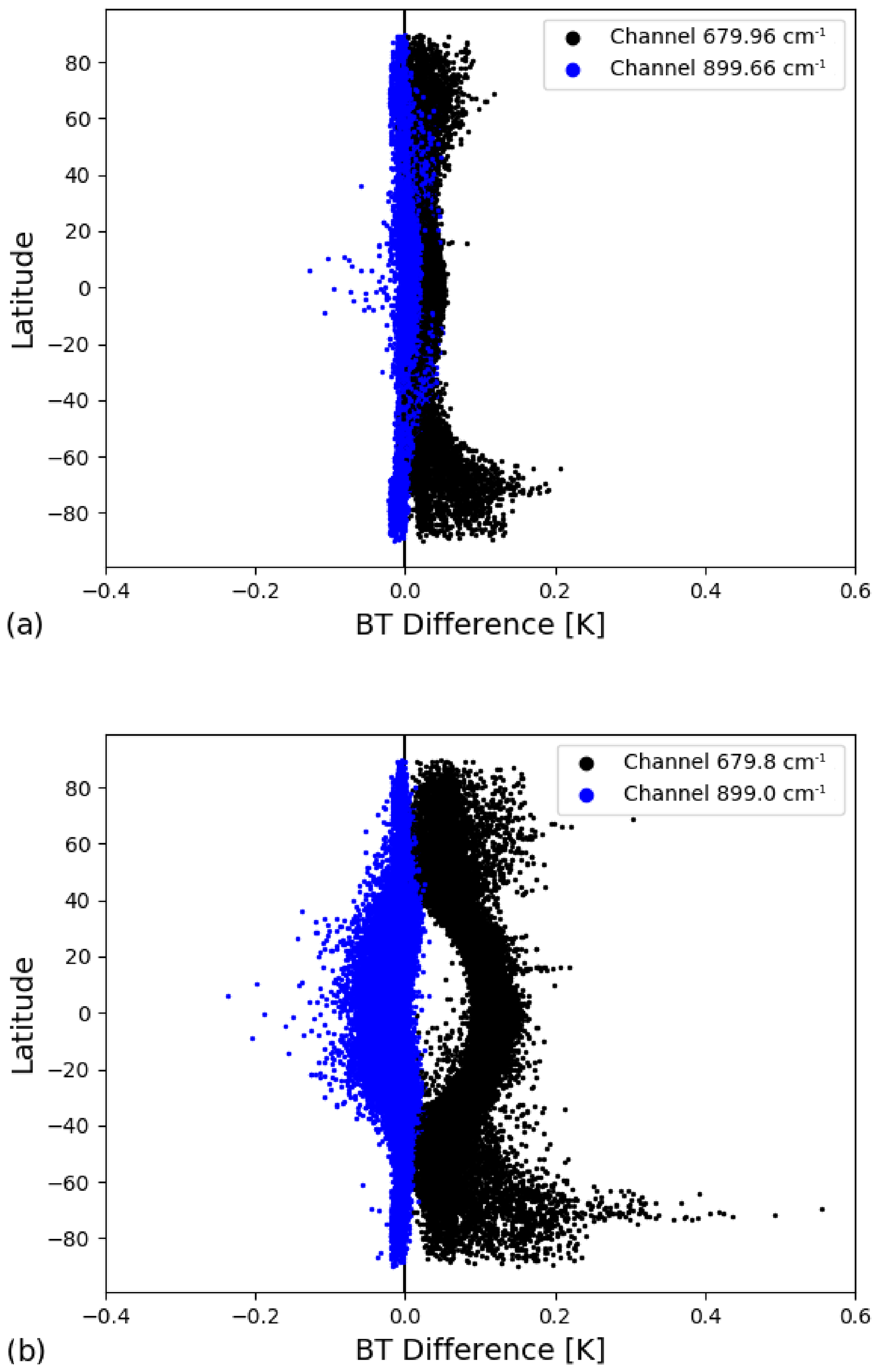
Figure 9 Latitudinal distribution of the difference between RTTOV and LBLRTM for each independent profile. (a) Channels centred at 679.96 cm⁻¹ (black circles) and centred at 899.66 cm⁻¹ (blue circles) from IRIS-D. (b) Channels centred at 679.8 cm⁻¹ (black circles) and centred at 899 cm⁻¹ (blue circles) from SIRS-B. Each point represents one of the 25 000 profiles.

For the infrared, three IRIS-D channels, two SIRS-B channels and one MRIR channel are shown. The three IRIS-D channels have corresponding channels on other instruments (two in SIRS-B and one in MRIR) which can be used to test the robustness of the results. These comprise one surface channel (centred at 899 cm⁻¹), one temperature (CO₂) channel (centred at 679 cm⁻¹) and one water vapour channel (centred at 1510 cm⁻¹). Figure 8 shows the spatial distribution of the difference between RTTOV and LBLRTM simulations for all independent profiles. Figure 8a and b represent the window channel centred at 899.66 cm⁻¹ from IRIS-D and SIRS-B, respectively. The IRIS-D spatial distribution presents a positive bias in the equatorial region and a negative bias in the polar regions. The maximum value reached is 0.05 K (Fig. 8a). For the corresponding window channel in the SIRS-B instrument at 899 cm⁻¹, a negative bias (around −0.04 K) is dominant in the equatorial regions but it is close to zero in the rest of the globe (Fig. 8b).

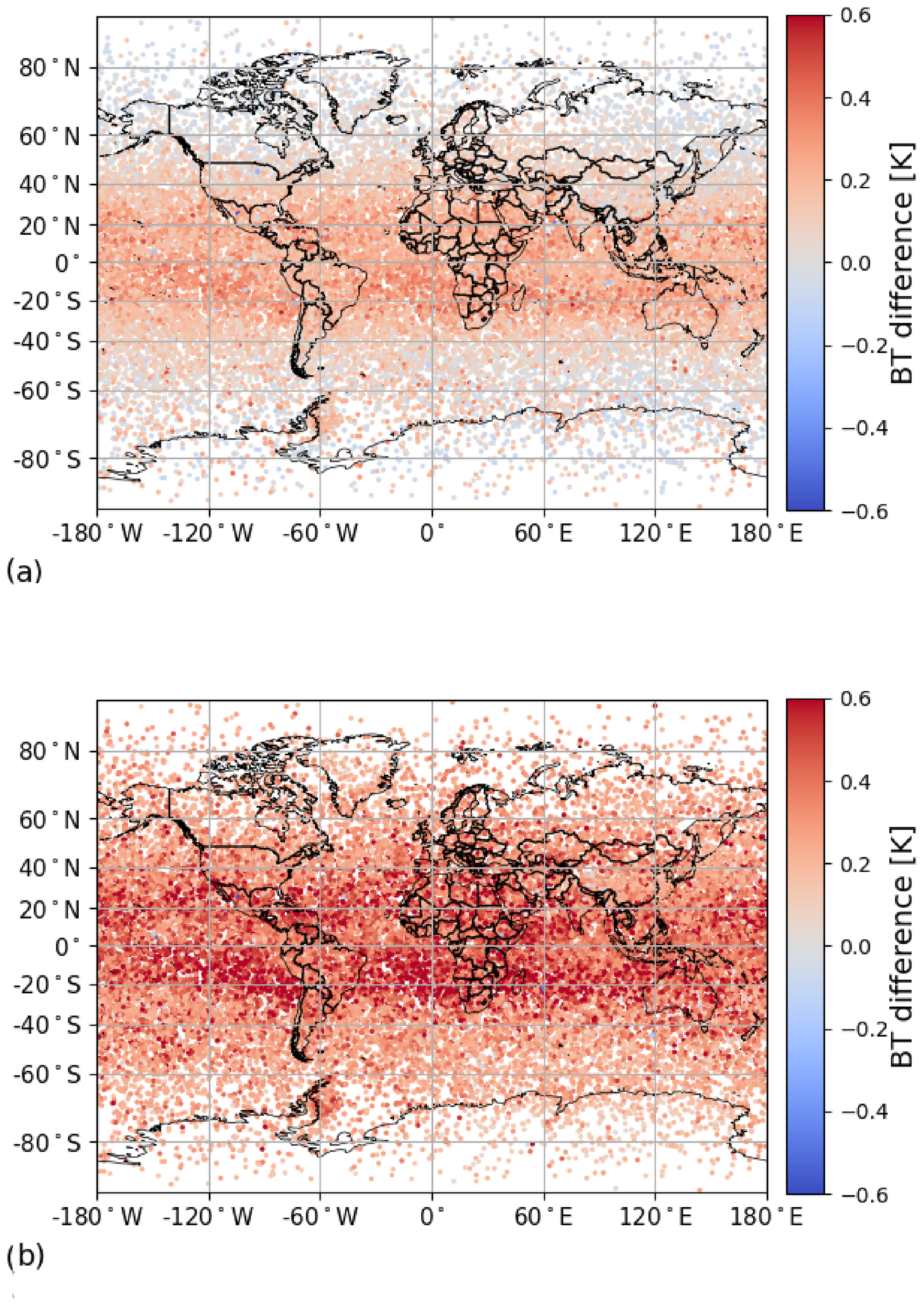
Figure 10 Spatial distribution of RTTOV minus LBLRTM for (a) the channel centred at 1510.11 cm⁻¹ from IRIS-D and (b) the channel centred at 1510.04 cm⁻¹ from MRIR. The profiles are from all five subsets.

Figure 9a shows the latitudinal distribution of the channels centred at 679 and 899 cm⁻¹ from IRIS-D, and Fig. 9b shows the same two channels from SIRS-B. The figure clearly shows that the bias has latitudinal behaviour. The channel centred at 899 cm⁻¹ tends to be negative in the equatorial region in the SIRS-B sensor (blue circles), whereas the corresponding channel in IRIS-D has a bias closer to zero, or slightly positive, in the equatorial region. To investigate this, we calculated the correlation between the mean bias and the integrated water vapour content (IWVC) that is provided for each of the 25 000 profiles. The correlation coefficient is moderate for both sensors; however, it is positive for the IRIS-D channel (0.48) and negative for SIRS-B (−0.47), mainly for the channel centred at 679 cm⁻¹ (black circles). The channel centred at 679 cm⁻¹ (black circles) presents a higher positive bias in all regions, the values are larger in the polar regions, and there is an increase in the differences from the extratropical regions to the equatorial region, which is more evident in SIRS-B. There is no correlation (0.017) between mean bias and the IWVC for the channel 679 cm⁻¹ of IRIS-D, and the correlation is 0.40 for the same channel of SIRS-B. The reason for these differences is not entirely clear, but as the only difference between simulations of the equivalent channels for both instruments is the bandwidth, with the SIRS-B channels being around a factor of 10 wider than those of IRIS-D, this is likely to be the cause. The spatial variability of the SIRS-A channels (figure not shown) is similar that of the SIRS-B channels.

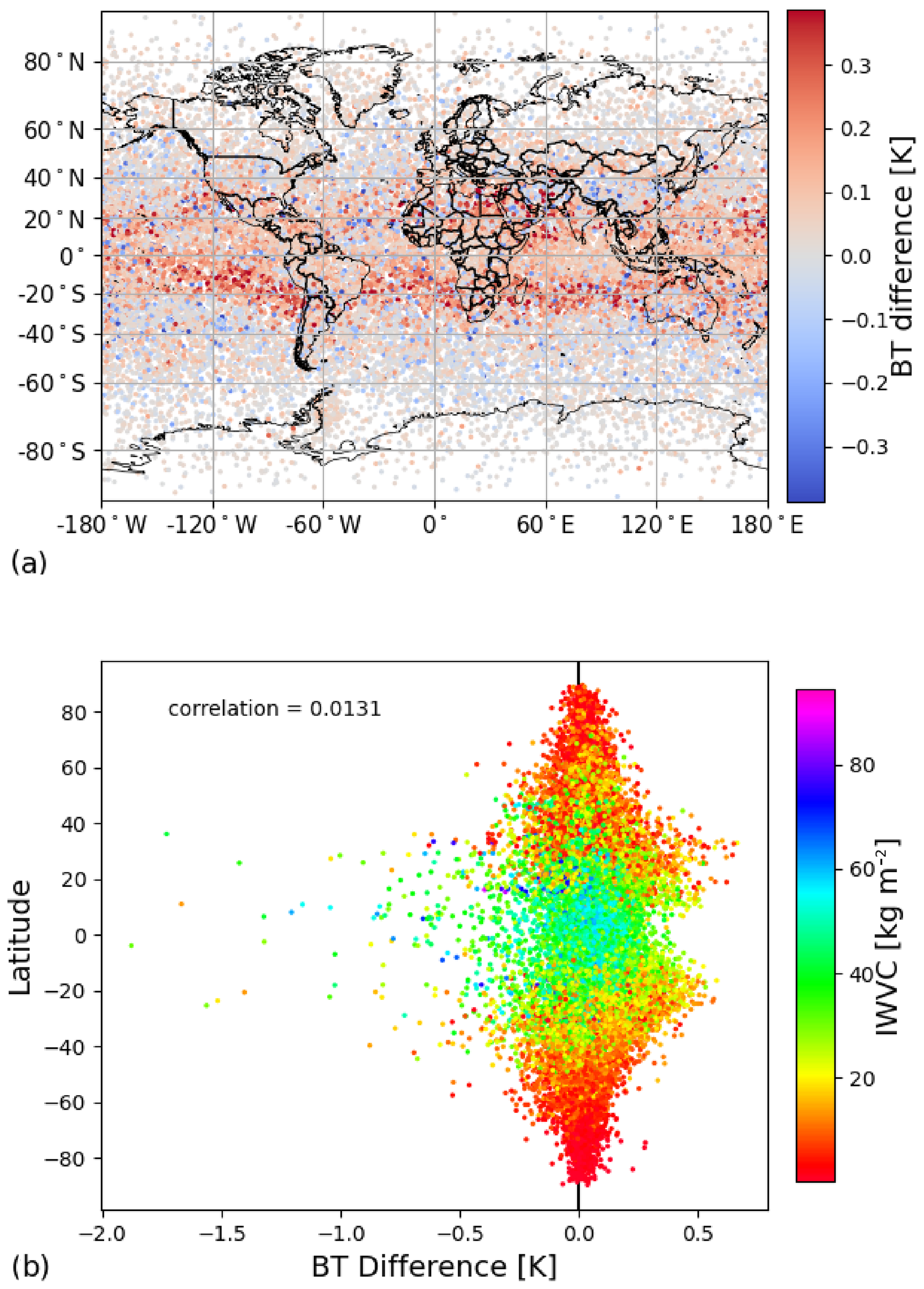
Figure 11 (a) Spatial distribution of RTTOV minus AMSUTRAN for channel 3 of SSM/T-2 at 183.31 + 1.0 GHz. (b) Latitudinal distribution of the difference between RTTOV and AMSUTRAN for each profile. The colour bar in (b) represents the integrated water vapour content (IWVC) from all five subsets.

A similar evaluation was made for one other channel from IRIS-D (centred at 1510.10 cm⁻¹) and one corresponding channel from MRIR (centred at 1510.03 cm⁻¹). Figure 10a and b show the spatial distribution of the water vapour channels centred at 1510 cm⁻¹ from IRIS-D and MRIR, respectively. Both channels present a positive bias in all regions, but there are a few points with negative bias (for example in the north of Mexico). The values are higher for MRIR, and it is possible to see a difference in intensity between the equatorial regions and the polar regions. IRIS-D presents positive values in the equatorial regions and a predominance of negative and close-to-zero values in the polar regions. In both cases, larger values are present in the equatorial region, which is possibly related to the content of water vapour in the atmosphere and its higher variability in these regions. There is no correlation (0.06) between mean bias and the IWVC for the channel at 1510 cm⁻¹ of IRIS-D, and the correlation is weak (0.23) for same channel of MRIR.

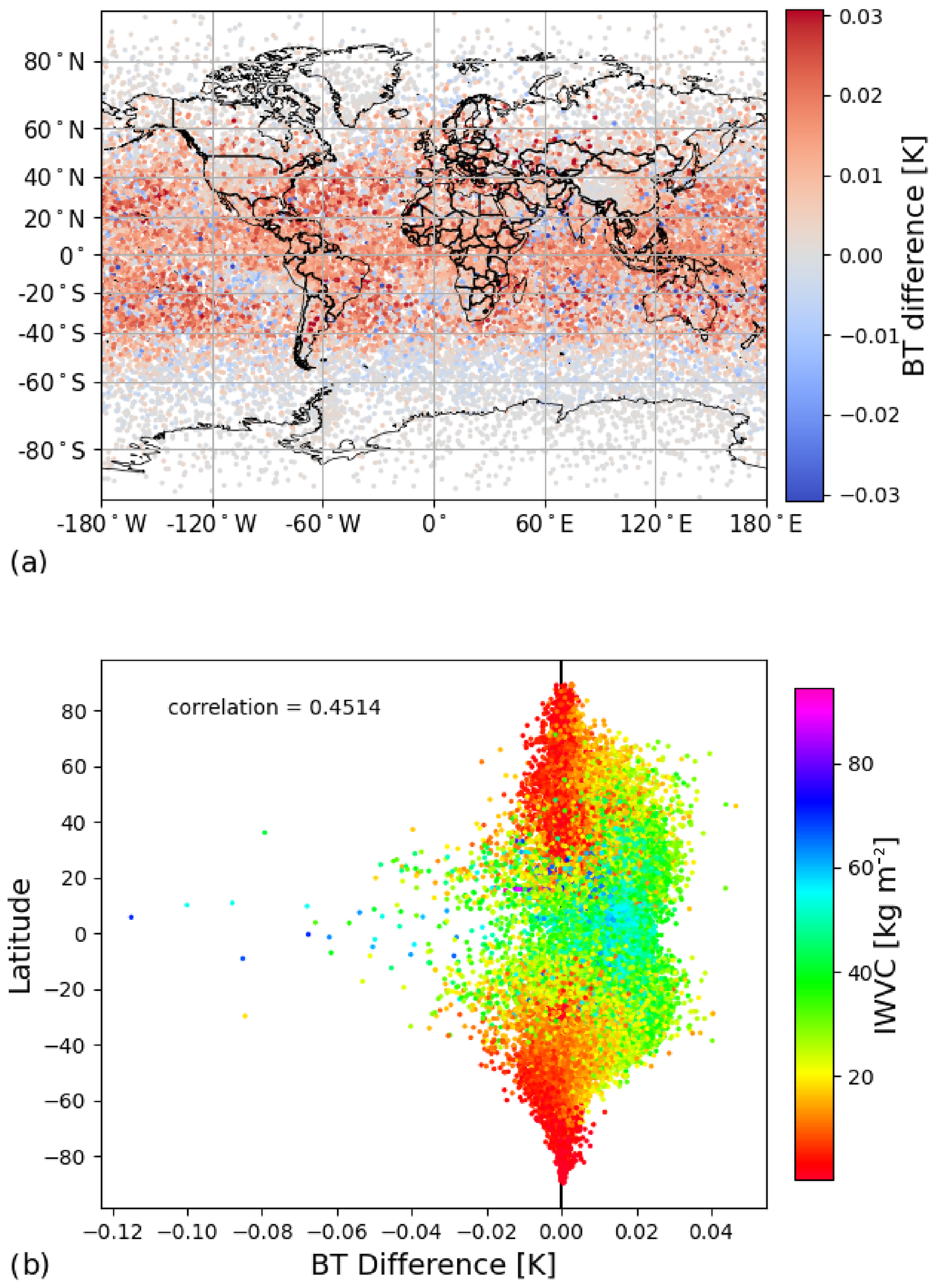
Figure 12 (a) Spatial distribution of RTTOV minus AMSUTRAN for channel 7 of SSM/I at 85.5 + 0.5 GHz. (b) Latitudinal distribution of the difference between RTTOV and AMSUTRAN for each profile. The colour bar in (b) represents the integrated water vapour content (IWVC) from all five subsets.

For the microwave, we examine the spatial distribution of the bias with channels sensitive to a range of features in the microwave spectrum: a water vapour channel centred at the 183.31 GHz line, a window channel at 85.5 GHz and a temperature channel centred at 60.79 GHz. The spatial bias distribution of the water vapour channel on SSM/T-2 with the closest proximity to the 183.31 GHz line (identical to channel 11 on SSMI/S) is shown in Fig. 11a, and the latitudinal distribution of the bias is shown in Fig. 11b. The bias appears to be strongest, up to about 0.5 K, in the subtropical belts (particularly the southern one) around 30^∘ N/^∘ S. The distribution of the bias around 0 K is reasonably symmetrical, but there are a few profiles with very negative biases around the equatorial regions, up to a maximum bias of nearly −2 K. This is possibly due to the unusual shape of the water vapour profile in the region of deep convective clouds, which could be challenging for the RTTOV predictors, but there is not a correlation between integrated water vapour content and bias (calculated value: 0.013), so this does not appear to relate to the vertically integrated amount of water vapour in total.

A similar story is seen for window channel 7 at 85.5 GHz on SSMI (Fig. 12), but with a far smaller magnitude. Apart from the surface, window channels will be affected only by the water vapour continuum (in the clear sky), whose contribution increases smoothly with frequency. The spatial pattern of positive bias is less concentrated in the subtropical belts and more broadly positive overall. In this channel, the very negatively biased equatorial profiles have slightly higher integrated water vapour contents than those with differences closer to zero. There is a slight to moderate correlation of 0.45. This pattern is detected in all microwave window channels with correlations of up to 0.49 at 37 GHz. Biases remain at 0.02 K or below for these channels in almost all cases.

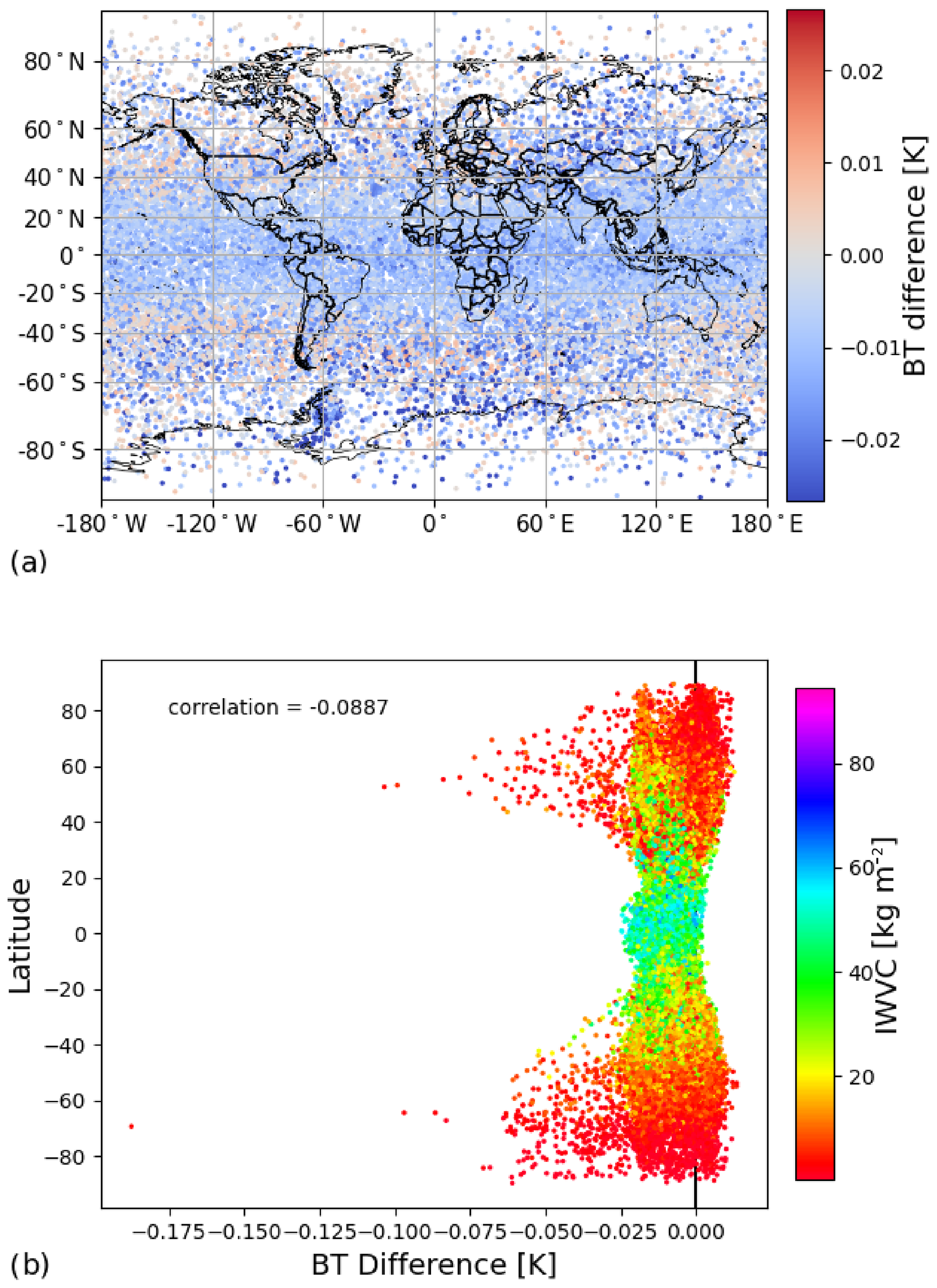
Figure 13 (a) Spatial distribution of RTTOV minus AMSUTRAN for channel 24 of SSMI/S at 60.79 + 0.36 + 0.05 GHz. (b) Latitudinal distribution of the difference between RTTOV and AMSUTRAN for each profile.

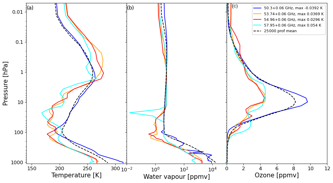
Figure 14 Atmospheric profiles of (a) temperature, (b) water vapour and (c) ozone for the profile identified as producing the maximum bias in each channel of MSU. The dashed black line is the mean of the 25 000 profiles. The legend shows the value of the maximum bias for each channel.

For the high-peaking temperature channels on SSMI/S, the pattern is quite different, see Fig. 13. The biases are mostly negative and less latitudinally variable apart from some stronger negative values around 60^∘ N/S. There is no correlation with IWVC, a feature that is seen with all microwave temperature-sounding channels that sense above the surface. The maximum difference is −0.18 K at 70^∘ S, but the value is anomalously low compared to the rest of the profiles. This feature is common among the channels: the maximum difference is far more extreme than for the vast majority of profiles. The profiles responsible for these extreme biases are examined in the following section.

5.3 Profiles associated with maximum bias

In order to examine the conditions under which the largest deviations between RTTOV and AMSUTRAN occur, the profiles associated with each channel's maximum bias are shown in Figs. 14–18 for each instrument in turn, and the locations of these profiles are shown in Fig. 19. As might be expected, some profiles are associated with multiple channels.

For MSU (Fig. 14), the profiles for the three higher-frequency channels 2–4 deviate significantly (lower) from the mean profile (dashed black line), whereas channel 1 at 50.3 ± 0.06 GHz is more similar. The profiles associated with channels 2–4 are located on the Antarctic Peninsula and the profile for channel 1 is over Australia; see Fig. 19. As these are all temperature-sounding channels, the unusually low values of temperature in the troposphere and stratosphere (Fig. 14a) are possibly outside of the range of the values the predictors are designed for, and the low stratospheric ozone values (Fig. 14c) likely contribute to this.

Figure 15 Same as Fig. 14 but for SSM/T-2.

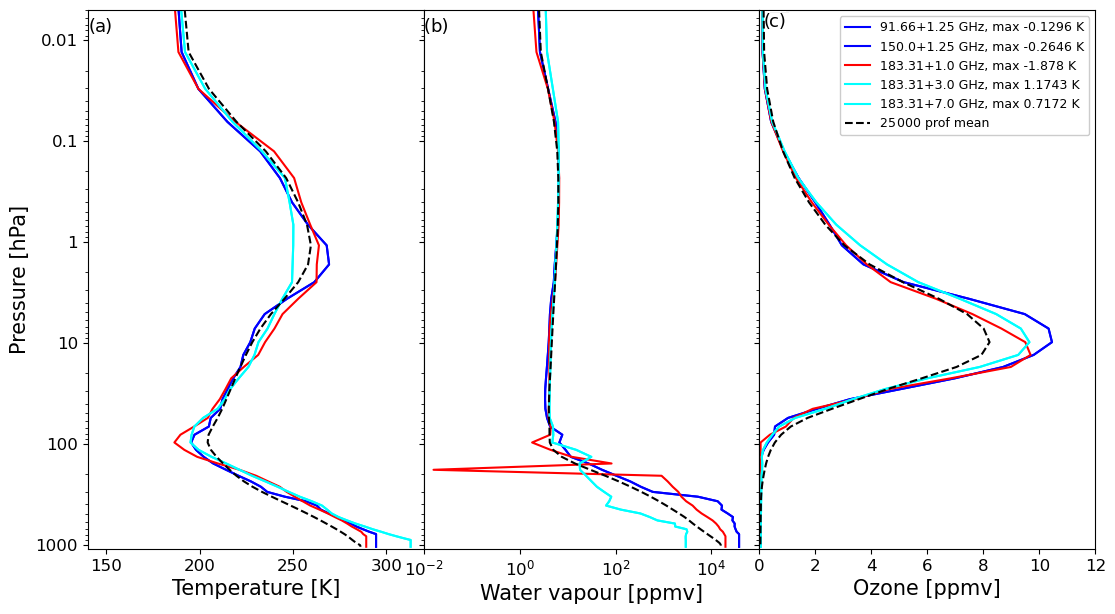
For SSM/T-2 (Fig. 15), the largest bias of −1.878 K comes from channel 3 at 183.31 ± 1 GHz, and the associated water vapour profile (Fig. 15b) shows a large anomalous spike from low water vapour in the upper troposphere around 200 hPa. The rest of the profile, however, is above the mean profile, particularly in the 200–300 hPa region, which may instead be the source of the bias. This profile is situated in the tropical Indonesian region. Two other profiles responsible for the biases in the four other channels are situated over Ethiopia and the Arabian Peninsula, the latter of which has a particularly dry profile.

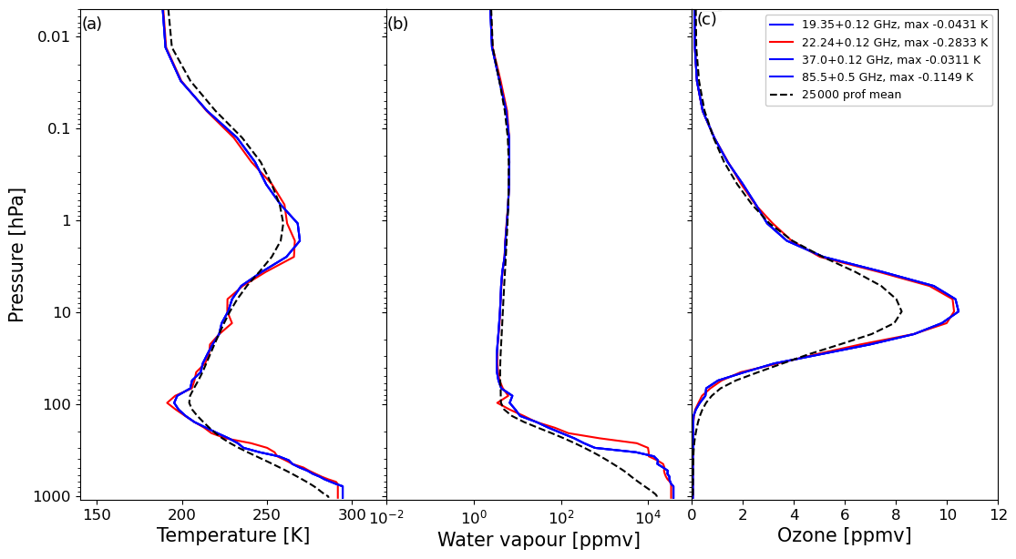
Figure 16 Same as Fig. 14 but for SSM/I. Only spectrally unique channels are shown as there is no difference between differently polarised channels with the simulation method used.

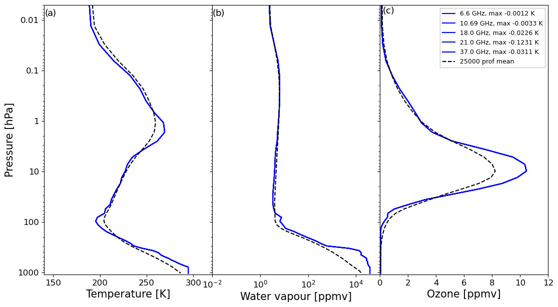
Figure 17 Same as Fig. 14 but for SMMR. Only spectrally unique channels are shown as there is no difference between differently polarised channels with the simulation method used.

The window channels on SSM/I (Fig. 16) are all similarly affected by the same high-humidity profile over Ethiopia, which also has high tropospheric temperatures and stratospheric ozone. Water vapour channel 3 (22.24 ± 0.12 GHz) has its highest bias associated with a profile that has higher water vapour at a slightly higher altitude and is situated 5^∘ north of the previous profile. All window/water vapour channels on SMMR (Fig. 17) are similarly most affected by the first Ethiopian profile. In total, half (25) of all the channels in the MW instruments considered are most affected by this profile.

Figure 18 Same as Fig. 14 but for SSMI/S channels 18–24 (high-peaking temperature channels).

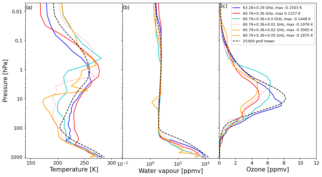
As the first 17 channels of SSMI/S are the same as channels on the other instruments, only the six unique high-peaking channels around 60 GHz are considered here. As can be seen in Fig. 18, the temperature profiles deviate strongly from the mean profile at upper levels between 400–0.01 hPa. The profiles associated with two of these channels have higher than average stratospheric temperatures and are situated over the Southern Ocean and Arctic, respectively. The remaining four channels have lower than average temperatures and are all situated over the Antarctic Peninsula.

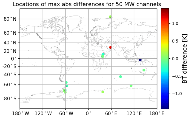
Figure 19 Global locations of the profiles responsible for each of the maximum biases for the 50 combined channels of the five MW instruments in this study. There are less than 50 points and some are associated with multiple channels.

6 Conclusions

The main objective of this study was to validate RTTOV coefficients using a large independent profile dataset for the historical infrared instruments IRIS-D, SIRS-B, MRIR and HRIR and the microwave instruments MSU, SSM/I, SSM/T2, SMMR and SSMI(S). The top-of-atmosphere (TOA) radiances are computed at high spectral resolution for a large profile dataset (the NWPSAF 137-level profile dataset interpolated to coefficient levels) using LBLRTM at nadir and AMSUTRAN at 6 standard satellite zenith angles. The LBLRTM TOA radiances convolved with the instrument ISRFs were compared against the RTTOV simulations for the infrared, whereas a top-hat/boxcar function was assumed for the passbands in the microwave region. The statistics of the comparison (mean, standard deviation and maximum) for the large profile dataset were then compared with the statistics of the profiles used to generate the RTTOV coefficients (dataset with 83 training profiles). The results for the infrared sensors showed that the statistics for the independent profile dataset (25 000 profiles) are similar to those found when using the 83 training profiles, indicating that the performance of RTTOV is robust for both datasets.

Differences between RTTOV and LBLRTM are higher in the water vapour channels, where the differences can reach 0.4 K (and up to 0.2 K for the standard deviation) in the independent profiles. In almost all the channels evaluated in this work, the training profiles show differences smaller than those for the 25 000 profiles. The maximum differences are also observed in these channels, and the values are higher in the independent profiles (up to 6 K). The latitudinal dependence of the bias is found in the channel centred at 679 cm⁻¹ from the SIRS-B instrument, and the range of the bias is higher for a multispectral instrument than for a hyperspectral instrument. Similar behaviour is observed in the MRIR channel centred at 1510 cm⁻¹. Those noticeable differences between channels on different instruments with similar central wavenumbers show the importance of the specification of the ISRF.

For the microwave sensors examined, the biggest differences between RTTOV and AMSUTRAN occur in water vapour channels, with means of up to 0.02 K (up to 0.1 K in standard deviation) in the training profile set; however, the validation with 25 000 profiles shows that this increases to 0.04 K (up to 0.13 K in standard deviation), which is still very low overall. Maximum differences in the training profile set reach −0.3 K in these channels, whereas a value of nearly −2 K was seen in the larger profile set; however, these very low values are extremely rare and are associated with profiles that significantly deviate from the profile mean and are located in regions with unique atmospheric conditions, such as deserts, the tropics or the polar regions. Even with these increased performance errors produced by the larger dataset in the water vapour channels, these values are still much smaller than the instrument errors that assimilation systems have to deal with. For example, the mean and standard deviation of the differences between observations and forecasted brightness temperatures are of the order of 0.5–1.5 K (https://nwp-saf.eumetsat.int/site/monitoring/nrt-monitoring/, last access: 7 February 2024) for SSMI/S channels 9–11, which are still in operation on NOAA-17.

Even though this study is restricted to historical sensors, the majority of which are no longer in operation, it confirms that the validation statistics for the 83-profile dataset are adequate to represent the overall biases for a range of different instruments. Equivalent statistics for all sensors supported by RTTOV can be found on the NWPSAF website (https://nwp-saf.eumetsat.int/site/software/rttov/download/coefficients/comparison-with-lbl-simulations/, last access: 7 February 2024) and can be used to provide an average bias correction. This study has further shown examples of the potential to exploit error predictors such as the satellite zenith angle, ice water content and spatial distribution of the differences, which may help with the development of the bias correction procedure applied to fast satellite simulations by identifying regions and scenes that challenge RTTOV during the reproduction of the line-by-line results. The next phase of the C3S project examines the covariances of these biases between channels.