Quantifying riming from airborne data during the HALO-(AC)³ campaign

Riming is a key precipitation formation process in mixed-phase clouds which efficiently converts cloud liquid to ice water. Here, we present two methods to quantify riming of ice particles from airborne observations with the normalized rime mass, which is the ratio of rime mass to the mass of a size-equivalent spherical graupel particle. We use data obtained during the HALO-(AC)³ aircraft campaign, where two aircraft collected radar and in situ measurements that were closely spatially and temporally collocated over the Fram Strait west of Svalbard in spring 2022. The first method is based on an inverse optimal estimation algorithm for the retrieval of the normalized rime mass from a closure between cloud radar and in situ measurements during these collocated flight segments (combined method). The second method relies on in situ observations only, relating the normalized rime mass to optical particle shape measurements (in situ method). We find good agreement between both methods during collocated flight segments with median normalized rime masses of 0.024 and 0.021 (mean values of 0.035 and 0.033) for the combined and in situ method, respectively. Assuming that particles with a normalized rime mass smaller than 0.01 are unrimed, we obtain average rimed fractions of 88 % and 87 % over all collocated flight segments. Although in situ measurement volumes are in the range of a few cubic centimeters and are therefore much smaller than the radar volume (about 45 m footprint diameter at an altitude of 500 m above ground, with a vertical resolution of 5 m), we assume they are representative of the radar volume. When this assumption is not met due to less homogeneous conditions, discrepancies between the two methods result. We show the performance of the methods in a case study of a collocated segment of cold-air outbreak conditions and compare normalized rime mass results with meteorological and cloud parameters. We find that higher normalized rime masses correlate with streaks of higher radar reflectivity. The methods presented improve our ability to quantify riming from aircraft observations.

1 Introduction

Mixed-phase clouds (MPCs) are a crucial part of the Arctic climate system. Observations have shown that MPCs occur about 40 % of the time (e.g., at Barrow, Alaska, or Ny-Ålesund, Svalbard; Shupe, 2011; Gierens et al., 2020), can persist up to several days (Zuidema et al., 2005), and can span hundreds of kilometers by forming organized cloud streets during cold-air outbreaks (Müller et al., 1999). MPCs play a critical role in the Arctic hydrological cycle and radiation budget, having, on average, a positive surface radiative forcing (Shupe and Intrieri, 2004; Kay and L'Ecuyer, 2013). However, the role of MPCs in a rapidly warming Arctic (Arctic amplification), where the mean near-surface air temperature has increased nearly 4 times more than the global mean over the last 4 decades (Rantanen et al., 2022), is not fully understood yet. It is unclear whether changes in MPC properties or frequency of occurrence will accelerate or decelerate Arctic amplification (Wendisch et al., 2023).

MPC properties are in part determined by microphysical processes. Supercooled liquid water (SLW) droplets can coexist with ice particles in MPCs between 0 and about −38 °C; at colder temperatures, homogeneous freezing occurs. Typically, MPCs are composed of a single stratiform layer or multiple stratiform layers of SLW near the cloud top and ice particles within and beneath the SLW layers (Shupe et al., 2006). While this composition is thermodynamically unstable, long MPC lifetimes are driven by a combination of various processes and feedback mechanisms that are poorly understood (Morrison et al., 2012). The representation of these processes poses a major source of uncertainty in numerical weather forecast and climate models (Morrison et al., 2020).

One important ice growth process, besides aggregation and depositional growth, common in MPCs is riming. Riming occurs when SLW comes into contact with ice particles, freezing onto them almost instantly. Typically, riming leads to denser, more spherical ice particles with increased mass, size, and fall velocity (Heymsfield, 1982; Erfani and Mitchell, 2017; Seifert et al., 2019). Due to its efficiency in converting SLW, riming is a key process for ice growth and subsequent precipitation formation. Moisseev et al. (2017) showed that, in Hyytiälä (Finland), riming was responsible for 5 % to 40 % of snowfall mass during winter 2014–2015, whereas Harimaya and Sato (1989) found riming proportions above 50 % for snowfall in a Japanese seaside area in 1987. Nonetheless, riming is often neglected in studies of Arctic MPCs (Avramov et al., 2011; Yang et al., 2013; Oue et al., 2016), especially in cases with low liquid water paths (LWPs). Fitch and Garrett (2022) showed in a recent study that riming is very common in Arctic low-level MPCs and also in cases of LWPs less than 50 g m⁻². Only 34 % of precipitating particles observed at Oliktok Point, Alaska, showed negligible amounts of riming. Fitch and Garrett (2022) proposed that riming enhancement can occur in regions with updrafts so that particles are exposed to SLW for a longer time span before falling out.

Riming has been studied in situ by airborne or ground-based measurements. Individual ice crystals or snowflakes that are observed manually (Harimaya and Sato, 1989; Mosimann et al., 1994) or by optical probes (Praz et al., 2017; Waitz et al., 2022) are often qualitatively classified. Mosimann (1995) was the first to quantify the degree of snow crystal riming using radar Doppler velocity measurements. They defined the riming degree on a scale from 0 to 5, where 0 means unrimed, 3 means heavily rimed, and 5 means graupel. Mason et al. (2018) retrieved a density factor as a proxy for riming from dual-frequency radar Doppler velocity measurements. Kneifel and Moisseev (2020) presented long-term statistics of the rime mass fraction (FR), the ratio of rime mass and snow particle mass, also obtained by Doppler velocity measurements, whereas Vogl et al. (2022) showed that FR can be predicted by an artificial neural network from radar reflectivity Z_e and skewness measurements. Previous studies have shown that collocating radar signals and in situ cloud data can be used to create, improve, and validate microphysical cloud retrievals (Tian et al., 2016; Trömel et al., 2021; Blanke et al., 2023).

In the Arctic, there are only a few observations of riming given the difficulty of (1) obtaining (quantitative) measurements of riming in general and (2) performing cloud measurements in remote regions. Airborne campaigns offer unique opportunities to measure in regions that are otherwise inaccessible. Waitz et al. (2022) showed observations of ice particles by optical probes collected during ACLOUD (Arctic CLoud Observations Using airborne measurements during polar Day, May–June 2017 – based in Svalbard, Wendisch et al., 2019). Images of ice particles are observed manually and qualitatively classified as unrimed, slightly rimed, moderately rimed, heavily rimed, and graupel. Nguyen et al. (2022) presented coincident triple-frequency radar and in situ observations obtained during the RadSnowExp (Radiation Snow Experiment, fall 2018 – based in Iqaluit, Canada; Wolde et al., 2019). They show close relationships between the triple-frequency signatures and in-situ-derived effective ice particle bulk density, which functions as a proxy for riming. Further, they compare to a machine learning ice particle habit classification that includes rimed categories. While both Waitz et al. (2022) and Nguyen et al. (2022) show the common occurrence of riming in Arctic MPCs and the high value of aircraft observations in studying riming, neither method can quantify the fraction riming contributes to particles' masses.

In this study, we present two methods to quantify riming from airborne measurements and apply them to data collected during the HALO-(AC)³ aircraft campaign (where “HALO” standards for High Altitude and Long Range Research Aircraft and “(AC)³” represents the “Arctic Amplification: Climate Relevant Atmospheric and Surface Processes, and Feedback Mechanisms” project; see https://halo-ac3.de, last access: 6 March 2024). HALO-(AC)³ took place in March–April 2022 with the main objective of studying Arctic air mass transformations and conducting collocated measurements with up to three aircraft. We focus on (collocated) remote sensing and in situ measurements obtained with the research aircraft Polar 5 and Polar 6, respectively. Both aircraft were based in Svalbard, and measurements were mainly collected over the open ocean and in the marginal sea ice zone (MIZ), the transition zone between open ocean and closed sea ice, west of Svalbard. We use the normalized rime mass M (Seifert et al., 2019), the ratio of rime mass to the mass of an equally large graupel particle, to quantify riming. The first method is based on an optimal estimation algorithm to obtain M from a closure between cloud radar and in situ measurements during collocated flight segments (combined method; see Sect. 3.1). We find M by matching measured radar reflectivities Z_e with simulated Z_e obtained from observed in situ particle number concentrations. The second method derives M from in-situ-measured particle shapes (in situ method; see Sect. 3.2). We compare results for M obtained with both methods for all collocated flight segments (Sect. 4.1). We then present a case study of a collocated flight segment from 1 April during cold-air outbreak conditions (Sect. 4.2) to show the performance of the two methods. Further, we investigate the relation of M to meteorological and cloud parameters such as temperature, liquid water content (LWC), total water content (TWC), LWP, and in-cloud location (Sect. 4.3). Lastly, we analyze all in situ data and evaluate how representative the collocated segments are for the whole campaign (Sect. 4.4).

2 Data

2.1 The HALO-(AC)³ airborne campaign

In this study, radar and in situ data from the HALO-(AC)³ campaign (Wendisch et al., 2024) are analyzed. During the campaign organized by the Transregional Collaborative Research Centre TR 172 (AC)³, three research aircraft were employed to study the Arctic atmosphere. The main objectives of the campaign included investigating warm-air intrusions into the Arctic and marine cold-air outbreaks (MCAOs) and collecting collocated measurements with up to three aircraft (Wendisch et al., 2024). The synoptic situation during the campaign is described in Walbröl et al. (2023). The instrumentation on board the Polar aircraft is similar to that used during the Airborne measurements of radiative and turbulent FLUXes of energy and momentum in the Arctic boundary layer (AFLUX) and the Multidisciplinary drifting Observatory for the Study of Arctic Climate – Airborne observations in the Central Arctic (MOSAiC-ACA) campaigns described in Mech et al. (2022a). During the majority of flights analyzed in this study, north and northeasterly wind transported cold-air masses from the central Arctic to the main measurement area in the Fram Strait.

We focus on data collected by Polar 5 and Polar 6, two Basler BT-67 aircraft operated by the Alfred Wegener Institute, Helmholtz Centre for Polar and Marine Research (AWI; Wesche et al., 2016). A total of 11 flights with Polar 5 and 13 with Polar 6 were conducted in March and April 2022 during HALO-(AC)³ in the vicinity of Svalbard. Closely collocated and nearly coincident measurements were obtained with the W-band cloud radar component of the Microwave Radar/radiometer for Arctic Clouds (MiRAC-A; Mech et al., 2019) on board Polar 5 and a variety of in situ cloud probes mounted under the wings of Polar 6 (Mech et al., 2022a). Figure 1a shows a conceptual sketch of how collocation was achieved: while Polar 6 was flying low and in-cloud, Polar 5 was following in close proximity on the same track above. The slight offset between the two planes was necessary so that dropsondes could be released safely from Polar 5.

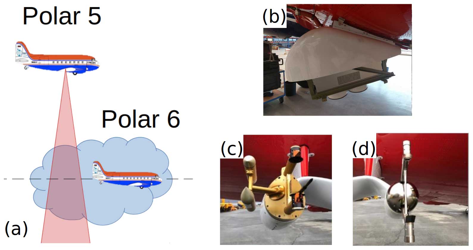
Figure 1 (a) Concept of collocation: while a radar on board Polar 5 is measuring the cloud from above, cloud probes on board Polar 6 simultaneously collect in situ samples at (almost) the same location inside the cloud. (b) MiRAC-A on Polar 5, located in its belly pot, and the wing-mounted cloud probes, namely the (c) Cloud Droplet Probe (CDP), Cloud Imaging Probe (CIP), and (d) Precipitation Imaging Probe (PIP), on Polar 6.

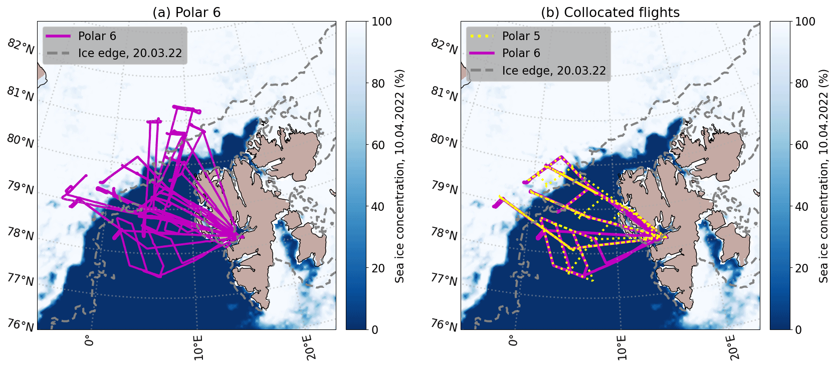
Figure 2 Flight tracks of (a) all Polar 6 flights (in situ) conducted during HALO-(AC)³ and (b) flights with collocated Polar 5 (remote sensing) and Polar 6 segments. The sea ice concentration (SIC) derived from the Advanced Microwave Scanning Radiometer 2 (AMSR2) on board the GCOM-W1 satellite on 10 April (at campaign end) is shaded in blue; the ice edge (15 % SIC) on 20 March (at campaign start) is shown in light gray.

Figure 2 shows (a) all flight tracks of Polar 6 and (b) flight tracks of both aircraft for flights with collocated segments. The overlapping lines show close spatial collocation. The sea ice concentrations (SICs) at the campaign beginning and end indicate the variable sea ice conditions. All 13 Polar 6 flights resulted in over 60 h of flight time and about 32 h of cloud particle measurements. A total of 31 % of the total flight time during the flights shown in Fig. 2b was conducted as collocated, which we define as both aircraft having a maximum horizontal distance of 5 km within a 5 min time window. From a total of about 11.8 h of collocated flight time, 4.6 h are collocated cloud measurements (this corresponds to a distance of approximately 1300 km assuming a typical speed of 80 m s⁻¹). The analyzed data cover a temperature range of −31 to −1 °C and an altitude range of in-cloud measurements from close to the ground to 1760 m.

2.2 In situ cloud probes

During HALO-(AC)³, a variety of in situ cloud data were collected. This study uses microphysical cloud data collected from three different cloud instruments, the Cloud Droplet Probe (CDP; Lance et al., 2010; Wendisch et al., 1996), the Cloud Imaging Probe (CIP; Baumgardner et al., 2011), and the Precipitation Imaging Probe (PIP; Baumgardner et al., 2011). All three probes were installed under the wings of Polar 6 (Fig. 1) and operated by the German Aerospace Center (DLR). The CDP is a forward-scattering optical spectrometer. The instrument measures cloud particles in the size range 2.8 to 50 µm by the intensity of forward-scattered laser light underlying Mie theory. Larger cloud particles are measured via optical array probes (OAPs). Here, two-dimensional shadow images of the cloud particles are recorded as the particles pass through the instrument's sampling area. The data collected by the CIP and PIP differ in pixel resolution. Both instruments consist of a 64-diode array, with the CIP covering a size range from 15 to 960 µm (15 µm resolution) and the PIP covering from 103 to 6.4 mm (103 µm resolution). By combining CDP, CIP, and PIP, a continuous particle size distribution is derived, including all hydrometeors from 2.8 to 6400 µm. We apply the same processing methods for the OAP data as those used for the AFLUX and MOSAiC-ACA campaigns (Moser and Voigt, 2022; Moser et al., 2022). The operating principles of the instruments, processing, uncertainties, and applied corrections are described in detail by Moser et al. (2023b) and Mech et al. (2022a).

Liquid water content (LWC) and total water content (TWC) were measured with a Nevzorov probe (Korolev et al., 1998). The probe was operated with a new sensor head, which featured an LWC sensor and two TWC cones with diameters of 8 and 12 mm (Lucke et al., 2022). The Nevzorov probe contains sensing elements which are regulated to provide a constant temperature (110 °C during the HALO-(AC)³ campaign). Droplets and ice particles momentarily cool the sensing elements when they impinge. In consequence, the sensors draw more power as they heat and evaporate impinging water in order to maintain their temperature, which can be used to estimate bulk LWC and bulk TWC. The measurement range of the Nevzorov probe extends from approximately 0.01 to 3.0 g m⁻³. Uncertainties of the Nevzorov depend very much on the atmospheric conditions that are present (Lucke et al., 2022). Nevzorov probe measurements made during HALO-(AC)³ are only available for flights in April due to technical difficulties in March. Air temperature was measured with a Pt100 mounted in a Rosemount housing at the noseboom of Polar 6. The measurements were corrected for adiabatic heating in the housing.

With the collected data, we are unable to distinguish between larger liquid droplets and small solid ice particles due to low-resolution images consisting of only a few pixels. We therefore assume all cloud particles with sizes larger than 50 µm to be ice crystals and all cloud particles with sizes smaller than 50 µm to be liquid droplets, similarly to Moser et al. (2023b). For the majority of low-level Arctic MPCs, this is appropriate to assume (McFarquhar et al., 2007; Korolev et al., 2017). This assumption is based on the good agreement between Nevzorov probe LWC and LWC calculated from the particle size distribution (PSD) assuming particles smaller than 50 µm to be liquid droplets where both measurements are available (R² = 0.83; Nevzorov and PSD LWC sum up to 973 and 983 g m⁻³, respectively, and lie within 1 % of each other). Additionally, we do not expect that this assumption will lead to significant biases due to radar reflectivities (that we simulate from in situ PSDs) being dominated by large particles.

2.3 Airborne remote sensing instruments

The Microwave Radar/radiometer for Arctic Clouds (MiRAC; Mech et al., 2019) was designed for operation on board the research aircraft Polar 5. During HALO-(AC)³ the active radar component (MiRAC-A) was operated on board Polar 5 in the same constellation as during MOSAiC-ACA. MiRAC-A is a 94 GHz frequency-modulated continuous-wave (FMCW) radar, which was mounted with an inclination angle of 25° backward in a belly pod under Polar 5. The radar measurements have been quality controlled and corrected for surface clutter, mounting of the instrument, and aircraft attitude (Mech et al., 2019). This results in georeferenced, regularly gridded data with a vertical resolution of 5 m (with reliable measurements starting 150 m above ground level due to ground clutter effects and 200 m distance from the aircraft for full overlap). Mech et al. (2019) estimate the accuracy of the radar reflectivity Z_e calibration to be 0.5 dBZ (neglecting attenuation). Because Doppler velocity measurements are biased by the aircraft motion, only Z_e measurements are used in this study.

The MiRAC-A radar is also equipped with a horizontally polarized 89 GHz passive channel using the same antenna as the radar. The brightness temperature (T_B) is also measured under a tilted angle of 25° backward to nadir. From this observation, the liquid water path (LWP) is estimated over open ocean only with a temporal resolution of 1 s, as described in Ruiz-Donoso et al. (2020). The retrieval takes profiles of nearby dropsondes to calculate T_B as a function of LWP measurements from simulations with the Passive and Active Microwave radiative TRAnsfer tool (PAMTRA; Mech et al., 2020). T_B (LWP) is approximated by a third-order regression. The regression is then applied in an inverse scheme to the 89 GHz T_B measurements to derive LWP. To eliminate biases in the observations, the differences between clear-sky and cloudy observations were used. Due to the variable microwave emissivity of sea ice, the LWP product is only available above open ocean.

Cloud top height (CTH) is obtained from the Airborne Mobile Aerosol Lidar for Arctic research (AMALi; Stachlewska et al., 2010), which was also operated on Polar 5. AMALi measures backscatter intensity profiles at 532 nm (polarized) and 355 nm (not polarized), from which the attenuated backscatter coefficient is calculated (Ehrlich et al., 2019). CTH is determined by searching for gradients in the backscatter coefficient.

For the present study, Z_e has been corrected for attenuation due to atmospheric gases and liquid hydrometeors. The two-way attenuation profile was calculated with PAMTRA. We used measurements from the closest dropsonde and the water vapor absorption model by Rosenkranz (1998) to calculate the attenuation due to water vapor for each time step. To estimate attenuation due to liquid water, we took LWC measurements from the Nevzorov probe operated on board Polar 6 during the temporally closest vertical cloud profile. To obtain information on the vertical structure of clouds, Polar 6 flew vertical profiles in so-called “saw-tooth patterns”. These patterns were flown in addition to straight legs at constant altitudes. Saw-tooth patterns are not well suited to making good-quality collocated measurements with Polar 5, where straight legs are preferred. Therefore, a limited number of vertical profiles are available for each flight with collocation. During each flight analyzed in this study, at least three such saw-tooth patterns were collected. Whenever Nevzorov probe measurements were not available, LWC was calculated by integrating the PSD of liquid particles (< 50 µm) measured with the cloud probes on board Polar 6. In both cases, LWC measurements were averaged to be on a regular vertical grid with a resolution of 10 m. Here, we neglect the distance traveled by Polar 6 during the profile, assuming LWC to be constant at each height bin. This assumption likely does not hold in reality; however, no measurements with more precise information on horizontal and vertical LWC distributions are available. Attenuation due to snowfall is assumed to be negligible compared to liquid droplets. During HALO-(AC)³, we obtain a mean two-way attenuation of 0.41 dB. By comparing integrated LWC measured with the Nevzorov probe and LWC calculated from PSD during cloud profiles (if both are available) to the temporally higher-resolved LWP from MiRAC-A, we estimate uncertainties of the attenuation correction to be 1 dB, leading to a total uncertainty of Z_e of 1.5 dB.

2.4 Collocation of radar and in situ measurements

In order to combine radar and in situ measurements, it is critical to have a temporally and spatially collocated data set. Following Chase et al. (2018) and Nguyen et al. (2022), the nearest radar data point to the in situ measurements is selected. We matched each 1 Hz Polar 5 data point with the spatially closest Polar 6 data point with a maximum horizontal distance of 5 km within a 5 min time window. Further, the radar range gate closest to the flight altitude of Polar 6 was chosen. Averaging radar reflectivity over certain height ranges close to Polar 6 did not lead to improvements. A rolling average of 30 s was applied to in situ data to obtain more robust statistics and to the radar data to make results comparable. Also, this is done to compensate for the different sampling volumes to a certain extent. While the radar footprint of a cloud in 2500 m distance is approximately 45.15 m in diameter, the cloud probes have measurement volumes in the range of a few cubic centimeters. We are aware that the assumption that the in situ measurement is representative of the entire matched radar volume is not always met and discuss possible implications of the assumption for our results in Sect. 5.

2.5 Simulated rimed aggregates

In addition to the observations, we use a data set of simulated rimed aggregates to relate particle properties and riming as discussed in Maherndl et al. (2023a). The aggregation and riming model described in Leinonen et al. (2013), Leinonen and Szyrmer (2015), and Leinonen and Moisseev (2015) is used in the setting “B” (aggregation followed by riming) to generate aggregates built from a predefined number of monomer crystals. The monomer crystal sizes are taken from an exponential size distribution, and the crystals themselves are composed of cubic-volume elements with an edge length of 20 µm. The aggregate sizes range from slightly below 100 µm to 12 mm. In this study, we only use dendrite monomer crystals, which is motivated by manual inspection of the in situ images for the collocated flight segments. After aggregation, the particles are exposed to a predefined amount of liquid water so that riming occurs. The frozen droplets that have rimed onto the ice particles are also represented by cubic-volume elements of 20 µm.

3 Methodology

Here, we describe how we obtain quantitative measures of riming in two different ways. To quantify riming, we use the normalized rime mass M (Seifert et al., 2019), which is defined as the rime mass m_rime divided by the mass of the size-equivalent spherical graupel particle m_g, where we assume a rime density of ρ_rime=700 kg m⁻³:

$$\begin{array}{}\text{(1)}& M={\displaystyle \frac{m_{\mathrm{rime}}}{m_{\mathrm{g}}}},\end{array}$$

where

$$\begin{array}{}\text{(2)}& m_{\mathrm{g}}={\displaystyle \frac{\mathit{\pi }}{\mathrm{6}}}{\mathit{\rho }}_{\mathrm{rime}}{D}_{\max }^{\mathrm{3}}.\end{array}$$

The definition of M implies M=0 for unrimed particles and M→1 for heavily rimed, spherical graupel particles. The maximum dimension D_max is defined as the diameter of the smallest circle encompassing the cloud particle (in m) and is used to parameterize particle sizes during the whole study (only for the in situ method, we convert D_max from physical units to pixel number).

First, we present an algorithm based on optimal estimation (Rodgers, 2000; Maahn et al., 2020) to retrieve average M of observed cloud particle populations for each time step from a closure of collocated remote sensing and in situ data (combined method; Sect. 3.1). Second, we describe the calculation of M based on in-situ-measured cloud particle shape. We use a data set of simulated rimed aggregates to relate particle shape to M and apply the method to in situ measurements of particle shape (in situ method; Sect. 3.2).

3.1 Combined method

We take advantage of collocated Polar 5 and Polar 6 flights and retrieve the average M of the observed cloud particle population value for each time step from the combination of radar and in situ measurements (Fig. 3).

Figure 3 Schematic of the retrieval framework.

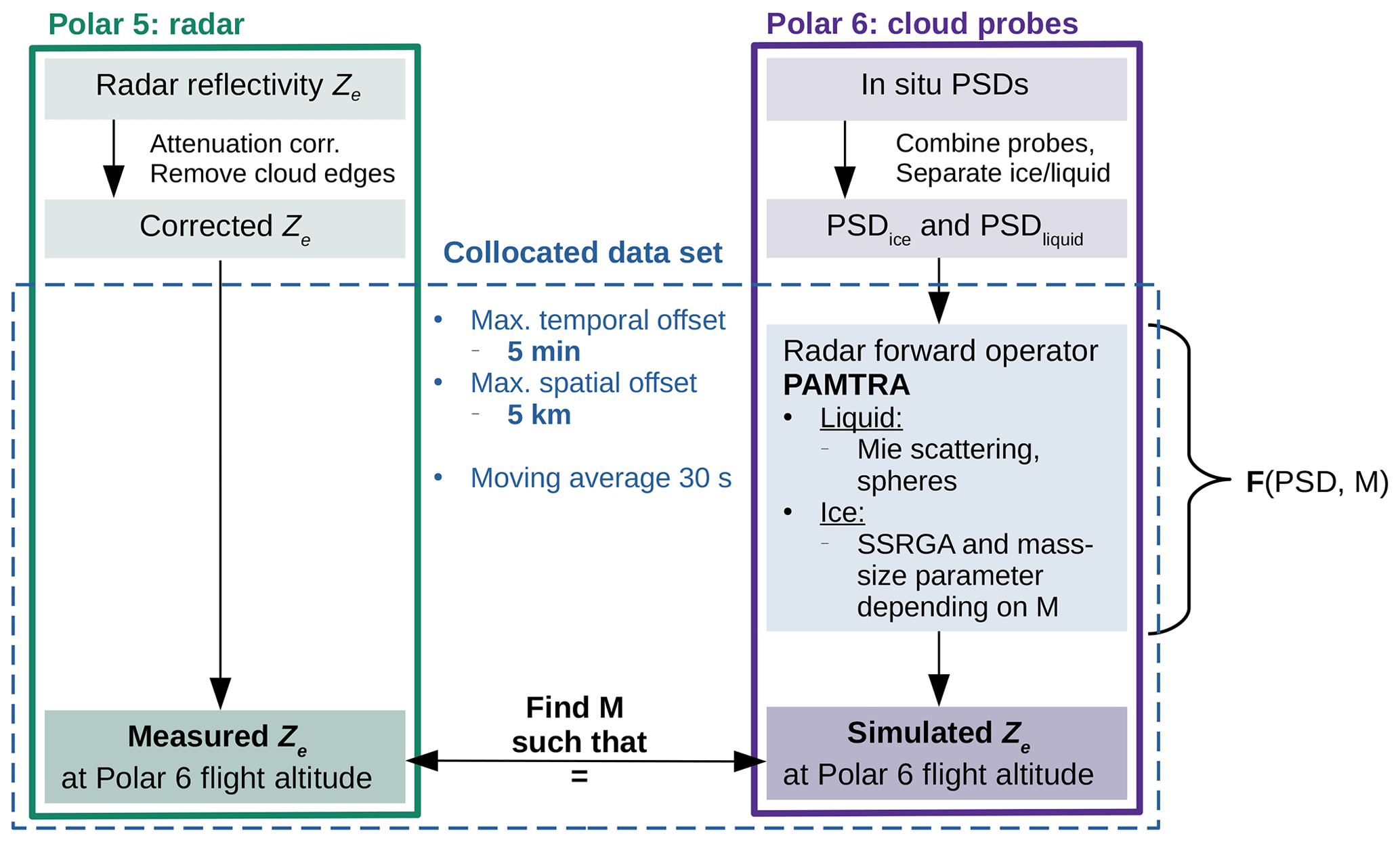
First, Z_e is corrected for attenuation (see Sect. 2.3), all cloud edges are removed to avoid non-uniform beam filling, and Polar 5 and Polar 6 data are combined (see Sect. 2.4). PAMTRA (Mech et al., 2020) is used to simulate Z_e from the in situ PSD and an initial guess for M. In principle, Z_e is a function of the mass, PSD, and scattering properties of the observed particle population. If the PSD is known and particle mass and backscattering are parameterized as a function of riming, M can be derived from a closure of Z_e and PSD. In the retrieval radar forward operator, we use Mie scattering (Mie, 1908) for liquid droplets. For ice particles, we use the self-similar Rayleigh–Gans approximation (SSRGA; Hogan and Westbrook, 2014; Hogan et al., 2017) and calculate the required SSRGA parameters from M with the empirical relations presented in Maherndl et al. (2023a). In addition, we consider the mass–size relation to follow a power law $\left(m=a_{\mathrm{m}}\cdot D_{\max }^{b_{\mathrm{m}}}\right)$, and we take the mass–size parameters a_m and b_m for dendrites from the same study. There, a_m and b_m are given for discrete M, so we interpolate a_m and b_m to obtain parameters for a continuous M. We discuss the assumption with regard to particle shape in Appendix A.

By parameterizing scattering, as well as mass–size relations, only by M and assuming that the measured PSDs are representative of radar measurements, we can tweak M until measured and forward-simulated radar reflectivities match within a given uncertainty range. This is done by optimal estimation (OE), a retrieval technique based on Bayes' theorem (Rodgers, 2000) implemented in pyOptimalEstimation (Maahn et al., 2020). OE uses a priori information x_a and a Gaussian statistical model to estimate the state vector x from the observation vector y in an iterative scheme. Starting with x_a as a first guess for x, the forward model F(x) (i.e., PAMTRA) is used to convert state to observation space. Then, the difference between y and F(x_a) is used to make a next guess for the state vector x₁, which requires inverting F(x) with the help of the Jacobian matrix $\mathbf{K}=\partial F\left(\mathit{x}\right)/\partial \mathit{x}$. This scheme is repeated until the a posteriori probability distribution $P\left(\mathit{x}\right|\mathit{y})=P(\mathit{y}\left|\mathit{x}\right)/P\left(\mathit{y}\right)$ reaches a maximum, resulting in the optimal x. This is achieved by minimizing the cost function J:

$$\begin{array}{}\text{(3)}& \begin{array}{rl}J& ={\left[\mathit{y}-F\left(\mathit{x}\right)\right]}^T{\mathbf{S}}_y^{-\mathrm{1}}\left[\mathit{y}-F\left(\mathit{x}\right)\right]\\ & +{\left(\mathit{x}-{\mathit{x}}_{\mathrm{a}}\right)}^T{\mathbf{S}}_{\mathrm{a}}^{-\mathrm{1}}\left(\mathit{x}-{\mathit{x}}_{\mathrm{a}}\right),\end{array}\end{array}$$

where S_y is the uncertainty of y (observation covariance matrix), and S_a is the a priori uncertainty (covariance matrix of x_a). Given that our problem is unambiguous (one measurement parameter y(Z_e) and one state parameter x(M)), using OE is not strictly necessary but has the advantage of providing uncertainties.

We choose x to represent M in common logarithmic scale (x=[log ₁₀(M)]) to avoid negative values. We use ${\mathit{x}}_{\mathrm{a}}=-\mathrm{1}$ (corresponding to M=0.1) as a priori information and S_a=1 as a priori uncertainty. We also evaluated different a priori guesses x_a and uncertainties S_a, but they lead to almost identical results and are therefore not shown; y refers to the attenuation-corrected Z_e measurements at Polar 6 flight altitude (in dBZ), and S_y represents the corresponding measurement uncertainty of 1.5 dB. Uncertainties due to non-exact collocation between Polar 5 and Polar 6 are neglected here. The average standard deviation of Z_e is 0.7 dB over distances of 555 m, which corresponds to the mean horizontal distance between the aircraft and is therefore smaller than the assumed uncertainty of 1.5 dB. In Sect. 4, we discuss implications of the non-exact collocation for the presented results. In Appendix B, we show that the OE output captures uncertainties of the combined method with synthetic data.

3.2 In situ method

The second method exploits the fact that riming impacts ice particle shape and typically leads to more spherical particles that can be derived from in situ image properties obtained by the CIP and PIP. This method can, in principle, be applied to all Polar 6 cloud particle measurements. From the captured images, hydrometeor properties described in the following were estimated. D_max, particle cross-sectional area A, and the perimeter area P are derived in the unit of pixel numbers. For the calculation of A and P, only particles that do not touch the edges of the OAP are used (Crosier et al., 2011). From A and P in the unit of pixel numbers, we calculate the complexity parameter χ, which we define as follows:

$$\begin{array}{}\text{(4)}& \mathit{\chi }={\displaystyle \frac{P}{\mathrm{2}\sqrt{\mathit{\pi }A}}},\end{array}$$

similarly to Gergely et al. (2017) so that χ of a sphere is 1. χ was originally proposed by Garrett and Yuter (2014), who included the inter-pixel variability (the variability in the brightness of one pixel compared to its neighbors) in their definition, which is not available for PIP measurements. Garrett and Yuter (2014) quantify riming based on χ, where rimed particles (graupel) are defined as χ≤1.35, moderately rimed particles are defined as $\mathrm{1.35}<\mathit{\chi }\le \mathrm{1.75}$, and aggregates with negligible riming are defined as χ>1.75.

A disadvantage of using χ to quantify riming is that it is a purely optical measure and not a physical quantity. Also, it should be taken into account that χ depends not only on a particle's shape (closely linked to its riming degree) but also on its size in a pixel. Depending on the resolution of the imager, as well as the exact definition of a perimeter pixel (continuous line vs. only touching outside), χ values of a circle with a diameter larger than 10 pixels can range from slightly below 0.9 to 1.3. Particle features finer than the resolution of the imager are not captured. This leads to smaller ratios of perimeter to area than for the same particle observed with a higher-resolution imager. For better visualization, the reader may imagine a fractal-shaped snowflake: the higher the resolution of the snowflake image, the larger the perimeter not only in pixel numbers but also when converting to a physical length. For any fractal shape, the length of the shape increases with increasing resolution, resulting in an infinitely large perimeter for an infinitely high resolution. In turn, larger particles have larger χ than smaller particles of the exact same shape captured by the same imager. Therefore, we take D_max, A, and P in the unit of pixel numbers to account for the different resolutions of CIP and PIP.

We use the same data set of simulated rimed aggregates from Maherndl et al. (2023a) to relate particle complexity χ and size to M. Only taking simulated aggregates of dendrites, we calculate χ from the average perimeter and area pixel counts over projections in the xy, yz, and zx planes, where one pixel corresponds to a square with 20 µm side lengths. We then derive an empirical relation with R² = 0.94 of χ depending on M and D_max in pixels, resulting in the following:

$$\begin{array}{}\text{(5)}& {\displaystyle }\begin{array}{rl}\mathit{\chi }& =\mathrm{1.33}-\mathrm{0.00243}\cdot {\log }_{\mathrm{10}}\left(M\right)\cdot D_{\max }+\mathrm{0.000171}\cdot D_{\max }\\ & -\mathrm{0.0854}\cdot {\log }_{\mathrm{10}}\left(M\right),\end{array}\text{(6)}& {\displaystyle }{\log }_{\mathrm{10}}\left(M\right)={\displaystyle \frac{\mathrm{1.33}-\mathit{\chi }+\mathrm{0.000171}\cdot D_{\max }}{\mathrm{0.00243}\cdot D_{\max }+\mathrm{0.0854}}}.\end{array}$$

χ is calculated from CIP- and PIP-measured P and A for each detected particle. M is then calculated from D_max and χ for each particle. To avoid unrealistic values, we set all log ₁₀(M)>0 to 0 and all ${\log }_{\mathrm{10}}\left(M\right)<-\mathrm{3.5}$ to −3.5. The latter threshold is chosen based on the minimum M of the results of the combined method.

By applying the relation derived for synthetic particles with a 20 µm resolution to CIP and PIP measurements with 15 µm and 103 µm resolution, respectively, we assume the ice particle shape to be fractal – i.e., χ only depends on D_max in pixels (and M) and not on D_max in a physical length unit. To check this assumption, we decreased the “resolution” of the synthetic ice particles to 60 µm by grouping together 3×3 pixels and applied Eq. (6). The resulting M bias is 27 % and is in the same range as using the original 20 µm particles (21 %).

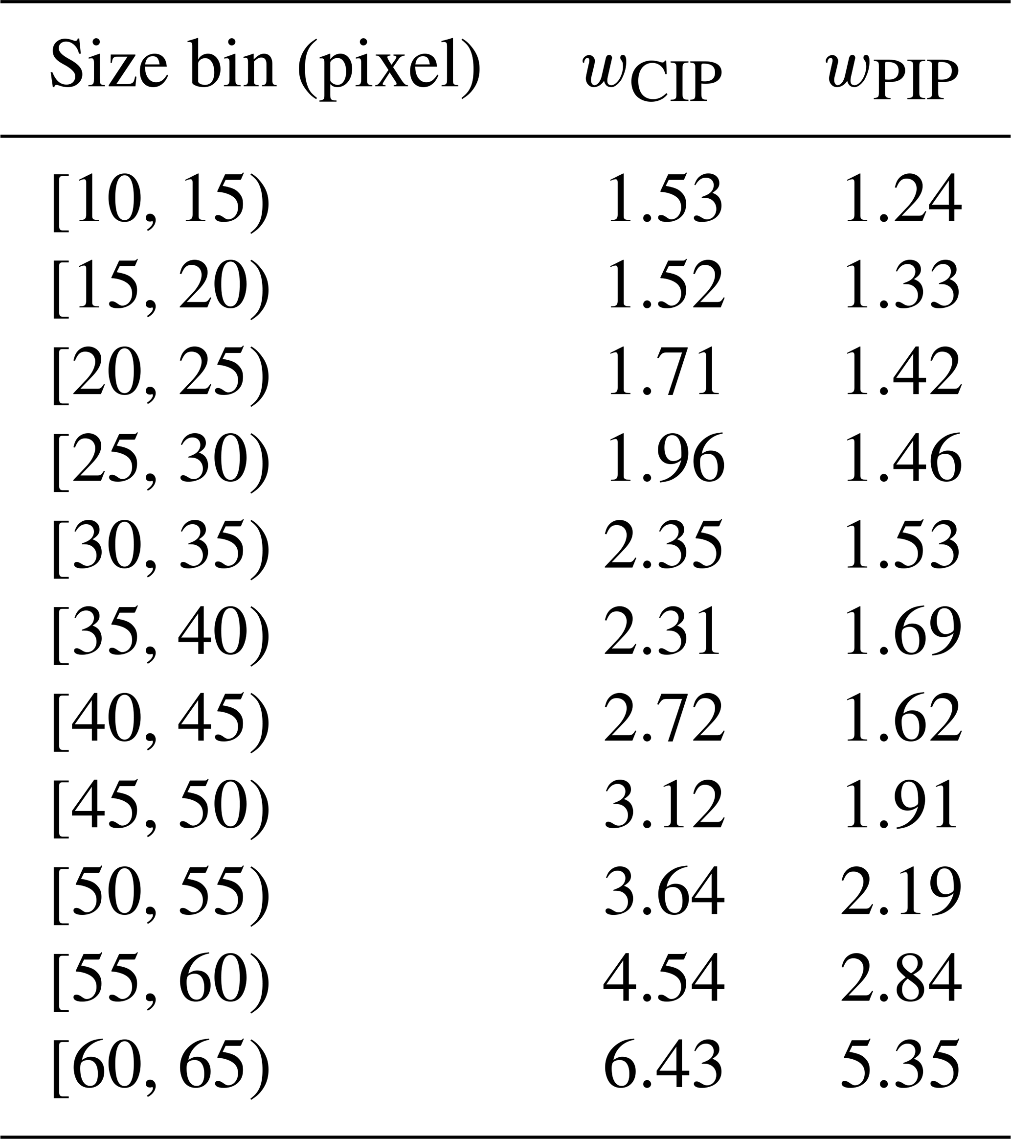
The detection efficiency of particles that do not touch the edges of the OAPs is size dependent: larger particles are more likely to touch the edge and are therefore less likely to be detected than smaller particles. To account for this, we derive weighting factors for CIP and PIP by comparing the count of total particles detected (including particles that touch edges) to the count of particles that do not touch edges. The weighing factors are derived for particle size bins from 10 to 65 pixels in five pixel bins (see Table C1 in Appendix C). From the calculated M, we obtain the weighted average for 1 s time steps. Then, a rolling average of 30 s (corresponding to 1.8–2.4 km for the typical Polar 6 flight speed of 60–80 m s⁻¹) is applied to make the results comparable with the M retrieval described in the previous section. We only consider particles with diameters larger than 14 pixels, which corresponds to 210 µm for the CIP and 1400 µm for the PIP. The threshold of 14 pixels was chosen such that 99 % of Polar 6 CIP- and PIP-measured particles with χ smaller than 1 lie below the threshold and are therefore sorted out for the analysis. χ values smaller than 1 are due to the low pixel resolution. This leaves us with a gap in the size range from about 1.0 to 1.4 mm. Evidently, only a subset of particles detected by CIP and PIP can be used to calculate M. Therefore, the in situ method can only be applied to a subset of the in situ data that are used for the combined method. This raises the question of how many particles per second is enough to achieve reasonable results assuming that high enough particle counts minimize the effects of the data gap. By comparison to the combined method, in addition to manual inspection of CIP and PIP images, we find that, in sum, at least seven particles per second need to be observed for reliably calculating M; thus, we discard data with lower counts.

We classify particles with M≥1.0 as heavily rimed (graupel; Fig. 4b). M values larger 1.0 are physically possible and indicate rime densities larger than assumed in the aggregation and riming model (ρ_rime=700 kg m⁻³). Particles with M<0.01 are classified as unrimed or having negligible riming due to their similar behavior to unrimed particles in Maherndl et al. (2023a). In between, we call particles with $\mathrm{0.01}\le M<\mathrm{0.1}$ lightly rimed and with $\mathrm{0.1}\le M<\mathrm{1.0}$ moderately rimed (Fig. 4b). In most cases, unrimed particles (Fig. 4a, left) have much more complex shapes and therefore larger χ than more heavily rimed ones (Fig. 4a, right), which are almost spherical (χ close to 1). Figure 4b shows the size dependency of χ. χ for the most heavily rimed particles, which reach M of about 0.87, is close to 1.33. Not shown are χ values of in-situ-measured cloud particles, which span values from about 0.7 to 5.0, with the majority of data (95 %) in the range of 1.0 to 3.0 for the CIP and 0.8 to 2.0 for the PIP.

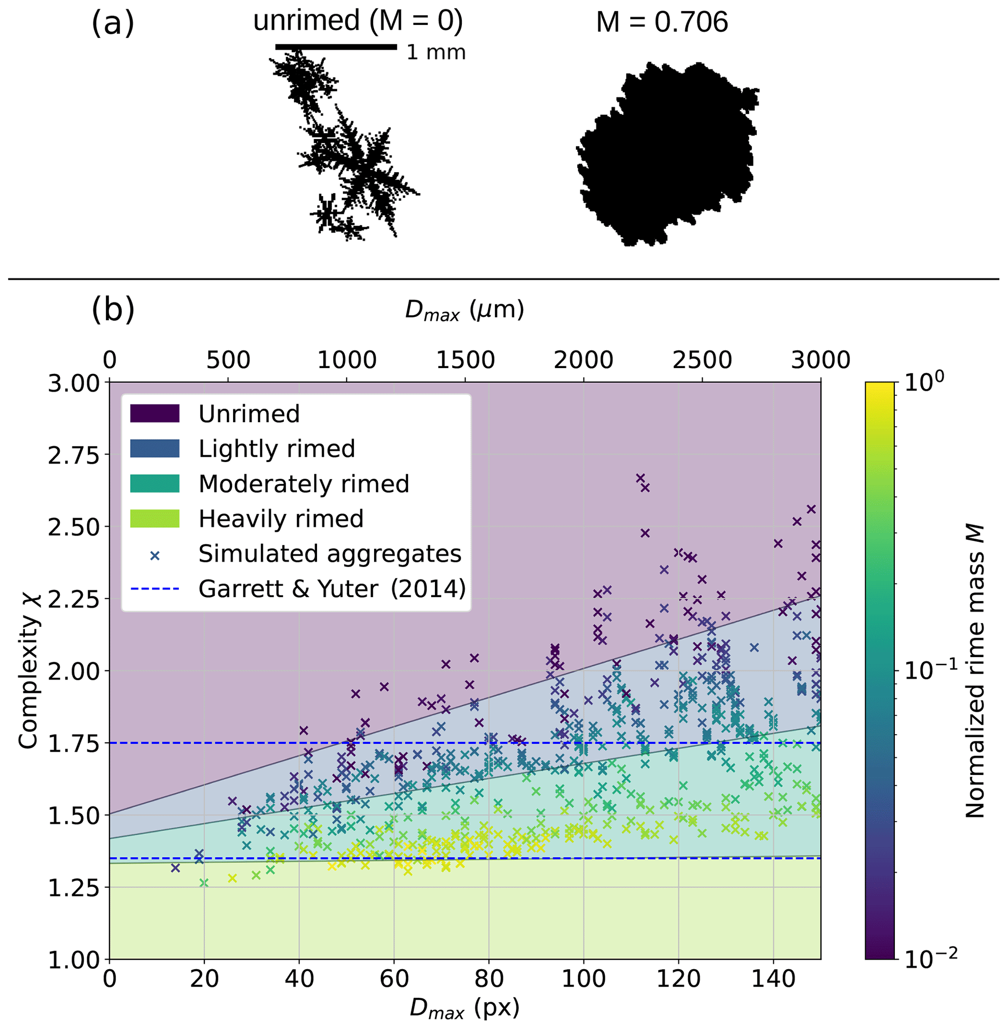
Figure 4 (a) Example simulated particles: unrimed dendrite aggregate (left) and moderately rimed dendrite aggregate (right). (b) Complexity χ of simulated dendrite aggregates with different amounts of riming versus their size D_max in pixels; 1 pixel corresponds to the resolution of the cubic elements (20 µm) that the simulated ice particles are composed of. Their normalized rime mass M is color coded. χ thresholds for graupel (1.35) and rimed particles (1.75) from Garrett and Yuter (2014) are included as dashed blue lines. Gray lines separating differently colored areas indicate isolines of M calculated with Eq. (6): M=0.01 between unrimed and lightly rimed, M=0.1 between lightly and moderately rimed, and M=1.0 between moderately and heavily rimed (graupel).

4 Results and discussion

To investigate the performance of both methods, we first compare M results for collocated flight segments showing agreement in a statistical sense (Sect. 4.1). Using a case study of a collocated flight segment, we discuss under which flight conditions agreement in a temporal sense can also be achieved (Sect. 4.2). Then, we relate M to meteorological and cloud micro- and macrophysical parameters (1) to further discuss possible biases of either method under certain conditions and (2) to study the occurrence of riming during collocated HALO-(AC)³ segments (Sect. 4.3). We then repeat the analysis for in situ method results derived for the complete Polar 6 data set (Sect. 4.4) to show that the subset of collocated flight segments is representative for the whole campaign, excluding low flight segments below 150 m.

4.1 Statistical comparison of both methods during collocated flight segments

Figure 5 shows a 2D histogram of combined and in situ method results of M for all collocated flight segments, as well as their respective M distributions. A high density of data points lies close to the 1 : 1 line, but data-point-per-data-point perfect agreement could not be achieved. However, the latter cannot be expected: although we match remote sensing and in situ data points as best as possible, there still remain offsets in time (less than 5 min) and space (less than 5 km). Additionally, radar and in situ probes have different measurements volumes.

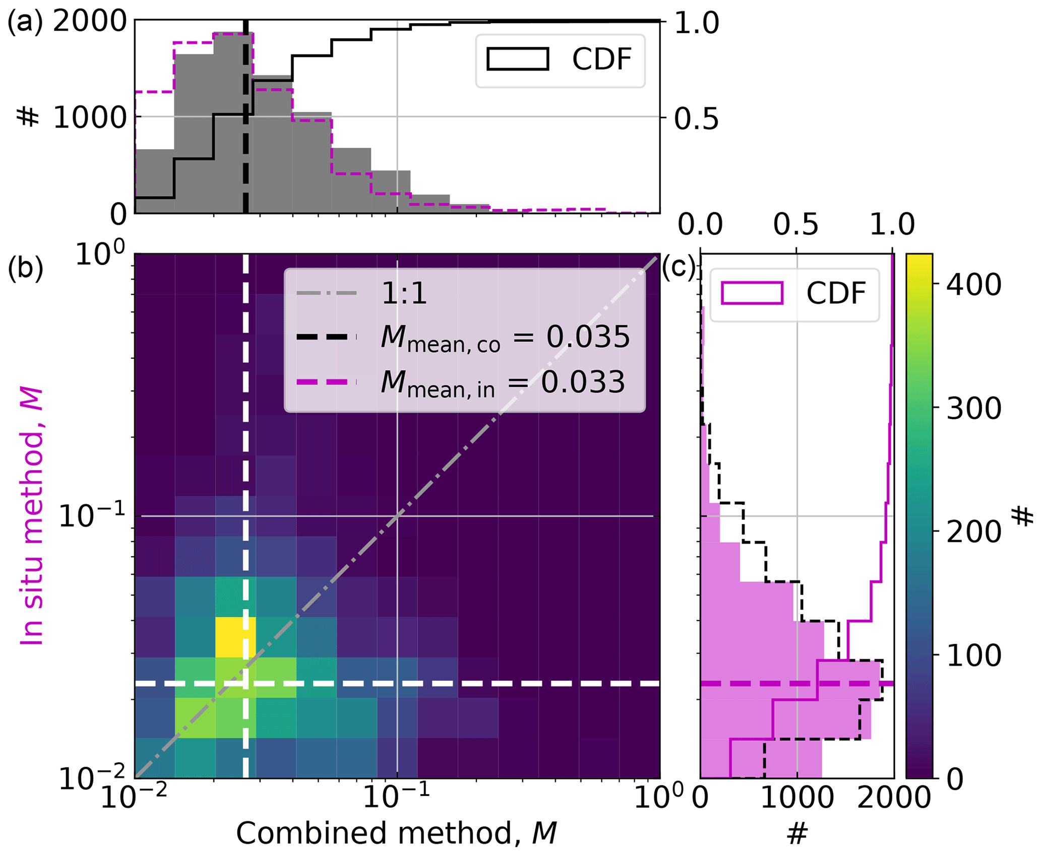
Figure 5 A 2D histogram of M derived with combined (x axis, black) and in situ (y axis, magenta) methods in logarithmic units during collocated flight segments. Individual histograms and cumulative distribution functions (CDFs) are included in black for the combined (a) and in magenta for the in situ method (c). Combined and in situ method histograms are also included as dashed lines in their respective color. Respective medians are plotted as dashed lines.

The respective distributions look very similar in shape, but combined method results are shifted to slightly larger values than with the in situ method. The mean of M is 0.035 and 0.033, the median is 0.021 and 0.024, and the 25 % to 75 % quantile ranges are 0.016 to 0.042 and 0.014 to 0.035 for the combined and in situ methods, respectively. The similarity, in addition to the close agreement of means, medians, and quantile ranges, gives us confidence that we achieve agreement with both methods and that both can be used to quantify riming. Mean error (ME) and root mean square error (RMSE) are 0.0026 and 0.031 for the point-by-point comparison. While we do not achieve good point-by-point agreement (large RMSE), both methods agree in a statistical sense (small ME).

Assuming particles with M<0.01 have negligible riming, we derive average rimed fractions of 88 % and 87 % over all collocated flight segments with the combined and the in situ methods, respectively. These numbers appear to be quite high. However, they depend heavily on the rimed vs. unrimed threshold that is chosen; if we assume M<0.05 to be unrimed instead of M<0.01, we get 11 % and 9 % rimed particles, respectively. We note that 12 % and 13 % of particles have M<0.01 for the combined and in situ method, respectively; 83 % and 83 % fall in the range $\mathrm{0.01}\le M<\mathrm{0.1}$; and only 5 % and 3 % have M≥0.1.

We see similar results when comparing the individual flights, except for 10 April (Fig. 6). Manual inspection of CIP and PIP images shows a high proportion of rimed particles during the collocated segment on 10 April (not shown), which is in agreement with the combined method. These particles appear to predominately have sizes around 1 mm – large enough to often touch edges in CIP images but too small to be able to calculate χ from PIP images. In all further analysis steps, we exclude the 10 April data, which correspond to 6 min of collocated data.

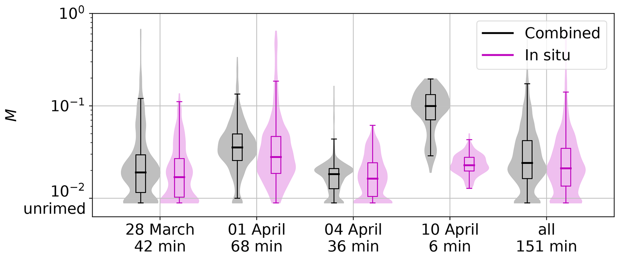
Figure 6 Box plots and superimposed violin plots showing distributions of M in logarithmic units derived with combined (black) and in situ methods (magenta) for collocated flight segments on the respective flight day and in total for all regarded collocations. Approximate collocated flight time in minutes is included.

4.2 Case study: collocated segment, 1 April

The good statistical agreement between both methods in combination with a rather large RMSE raises the question of why agreement in terms of temporal confluctuations could not be achieved for all flight segments. In the following, we use a case study to demonstrate under which conditions combined and in situ methods agree on a data-point-per-data-point basis and discuss possible biases of both methods.

A high-pressure system north of Greenland and a strong low-pressure complex north of Siberia lead to northerly and northeasterly winds almost parallel to the ice edge in the Fram Strait, where the measurements were performed. The movement of cold air from the colder sea ice north of the Fram Strait to the warmer ocean resulted in the formation of cloud streets, which can be seen in Fig. 7a. Walbröl et al. (2023) identified this cold-air advection as a strong marine cold-air outbreak (MCAO) that lasted from 1 to 2 April. On 1 April, Polar 5 and Polar 6 conducted collocated flights, crossing the Fram Strait perpendicular to the cloud streets from 7.6 to 1.5 ° E, traveling back and forth three times. Clouds were thicker, more pronounced, and extended higher over the open ocean on the eastern side of these segments than close to the MIZ and were absent over sea ice. Polar 5 stayed at a constant altitude of 3 km, while Polar 6 performed predominately staircase patterns, measuring in and above clouds. Here, we show a short segment where Polar 6 flew inside clouds from west to east on the eastern side of the measurement area close to 7.6 ° E, while Polar 5 flew above. Then, both aircraft turned and flew the same way back westward. Excluding the turn, the horizontal distance between both airplanes ranged from 48 m to 2.7 km and was, on average, 1.2 km.

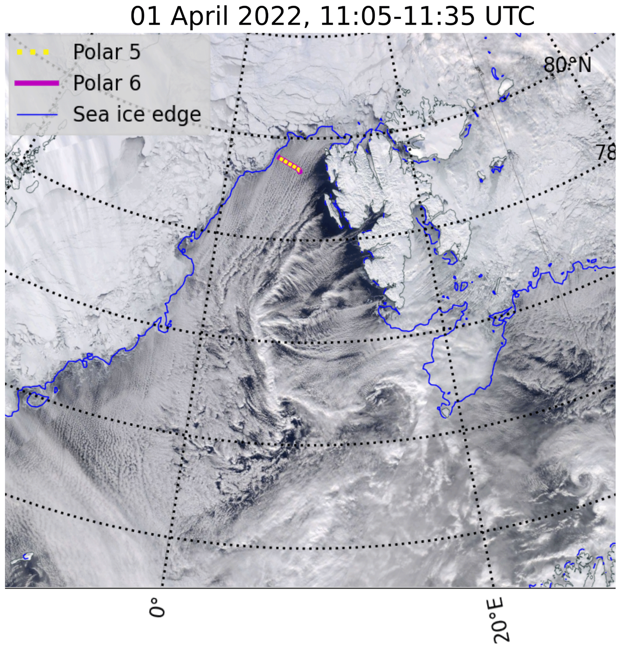
Figure 7 MODIS Terra reflectance images (NASA Worldview, 2024) from 1 April. The flight tracks of Polar 5 (yellow) and Polar 6 (magenta), as well as the sea ice edge (15 % SIC), of the same day are included.

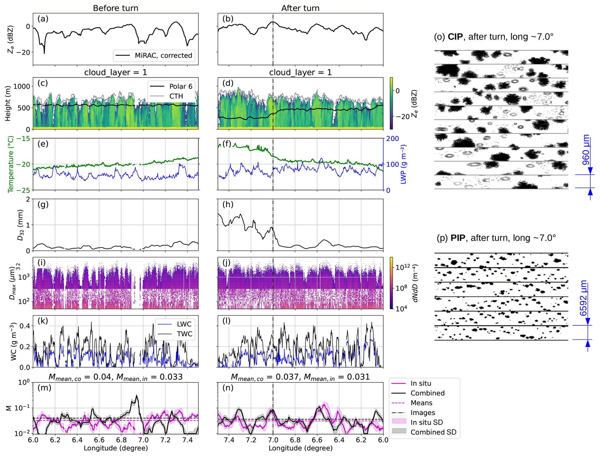
Figure 8 Collocated flight segments from 1 April 11:05–11:35 UTC before (first column) and after turn (second column). The longitude axis is reversed for the after-turn segment to visualize time passing on the x axis. (a–b) MiRAC-measured and MiRAC-corrected reflectivity Z_e in the flight altitude of Polar 6; (c–d) MiRAC-measured reflectivity Z_e, AMALi CTH, and Polar 6 flight altitude; (e–f) Polar 6 noseboom temperature (green) and MiRAC-A LWP (blue); (g–h) mass-weighted diameter D₃₂ derived from the 30 s running average combined and in situ PSD; (i–j) CIP- and PIP-measured combined PSD (not averaged); (k–l) Nevzorov probe LWC (blue) and TWC (black); (m–n) M from combined (black) and in situ methods (magenta) including uncertainty estimates (combined: OE standard deviation, in situ: 30 s running standard deviation); (o) example CIP; (p) PIP images from 7° E after the turn as indicated by the dash-dotted line in panels (b), (d), (f), (h), (j), (l), and (n).

A detailed view of collocated in situ and radar measurements during this segment is presented in Fig. 8. The first column shows measurements before the turn (aircraft flying from west to east, about 11:08 to 11:18 UTC), while the second column shows measurements after the turn (east to west, about 11:25 to 11:35 UTC). We cut out the turn due to unreliable measurements and/or collocation matching when the radar is tilted due to the aircraft roll. In-cloud temperatures decreased with height, ranging from −22 to −15 °C in the measured area (Fig. 8e and f). The cloud's roll structure is clearly visible in the radar measurements: Z_e shows periodic streaks of high and low values (Fig. 8c and d), which can also be seen in the averaged (moving over 30 s), corrected Z_e at the altitude of Polar 6 (Fig. 8a and b). D₃₂ is the proxy for the mean mass-weighted diameter (e.g., Maahn et al., 2015) and is defined as the ratio of the third to the second measured PSD moments $M_{\mathrm{3}}/M_{\mathrm{2}}$ assuming a typical value of 2 for the exponent b of the mass–size relation (e.g., Mitchell, 1996). D₃₂ calculated from the 30 s running average of the combined in situ PSD (Fig. 8g and h) and the PSD (Fig. 8i and j) shows gaps when Polar 6 was flying close to cloud top (before the turn), and streaks of high Z_e appear to correlate with increases in D₃₂. Nevzorov probe measurements (Fig. 8k and l) show that the sampled cloud was mixed-phase, with LWC being, in general, slightly higher close to the cloud top.

We see good agreement when looking at mean, median, and quantile ranges of M derived with combined and in situ methods before and after the turn. The combined method results in a median (mean) M of 0.031 (0.040) before and 0.032 (0.037) after the turn, while the in situ method gives a median (mean) M of 0.031 (0.033) before and 0.022 (0.031) after the turn. The 25 % to 75 % quantile ranges are 0.022 to 0.044 and 0.024 to 0.042 for the combined method before and after the turn, respectively. Quantiles range from 0.021 to 0.043 and 0.018 to 0.036 for the in situ method.

However, when comparing the time series of M, we see a much better agreement in terms of temporal confluctuations after the turn compared to before. We assume that the discrepancy before the turn is due to the Polar 6 measurements being close to the upper edge of the cloud. As discussed in Appendix D, agreement between both methods is worse close to the highest radar range gates with cloud signals. This is likely due to the higher spatial variability and larger spatial gradients of cloud properties. Even slight horizontal offsets of Polar 5 and Polar 6 in addition to the different measurement volumes of radar and cloud probes can result in disagreements between radar and in situ probes. Close to the upper edge of the cloud, this can result in the radar detecting a gap in clouds while the in situ probes measure a particle concentration larger than zero or vice versa. Apparently, the running averages of 30 s in both data sets cannot completely resolve this problem. In addition, median particle count increases from 17 before the turn to 22 after the turn, resulting in the in situ method being less reliable before the turn as well. Therefore, near the cloud top, both methods are less reliable in a spatio-temporal sense. They do, however, both produce reliable estimations of M in a statistical sense.

After the turn, combined and in situ results for M show better agreement as Polar 6 was flying deeper in-cloud under more homogeneous conditions. Both methods show an almost periodic increase and decrease in M, with (almost) matching maxima and minima in terms of extent and location. Compared to Z_e (Fig. 8b and d), high M values correlate with high Z_e, indicating that riming plays a dominant role in MPC variability, as observed by radar.

CIP and PIP images taken at 7.0 ° E after the turn are presented in Fig. 8o and p and show a mixture of small liquid drops, pristine plates, and a high proportion of rimed (aggregated) dendritic ice particles, explaining the peak in M for both methods.

4.3 Occurrence of riming during collocated flight segments

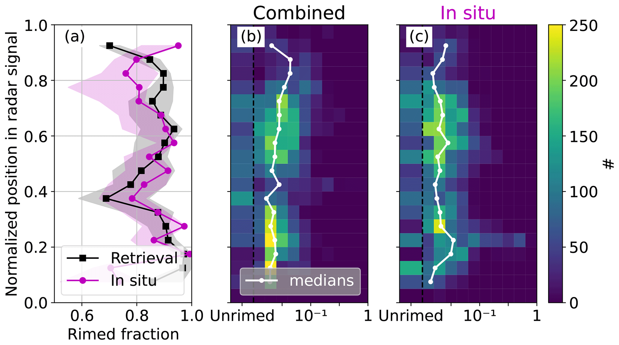
Figure 9 gives an overview of the occurrence of riming depending on (a–d) Polar 6 noseboom measurements of air temperature T; (e–h) Nevzorov probe LWC; (i–l) Nevzorov probe TWC; (m–p) MiRAC-A-retrieved LWP; and (q–t) the normalized position of Polar 6 in cloud, which we define as the fraction of Polar 6 flight altitude minus cloud bottom height (CBH) and CTH minus CBH (therefore, cloud bottom = 0 and cloud top = 1). CTH is determined from AMALi, while CBH is determined from radar measurements, where cloud bottom is the lowest Z_e measurement not affected by ground clutter. If there is a continuous signal from 150 m to the flight altitude of Polar 6 then cloud bottom is set to 150 m. Note that the liquid cloud base, which is commonly used when using ground-based remote sensing, is not available for airborne measurements. Our cloud definition includes precipitation falling out of the cloud liquid layer so that multi-layer clouds connected by precipitation would be treated as a single cloud. During the collocated flight segments used in this study, no separate cloud layers were observed by the radar above Polar 6. The average rimed fractions derived with both methods show a similar behavior for all parameters and lie, on average, within 6 percentage points of each other. Linear medians match within a factor of 0.3.

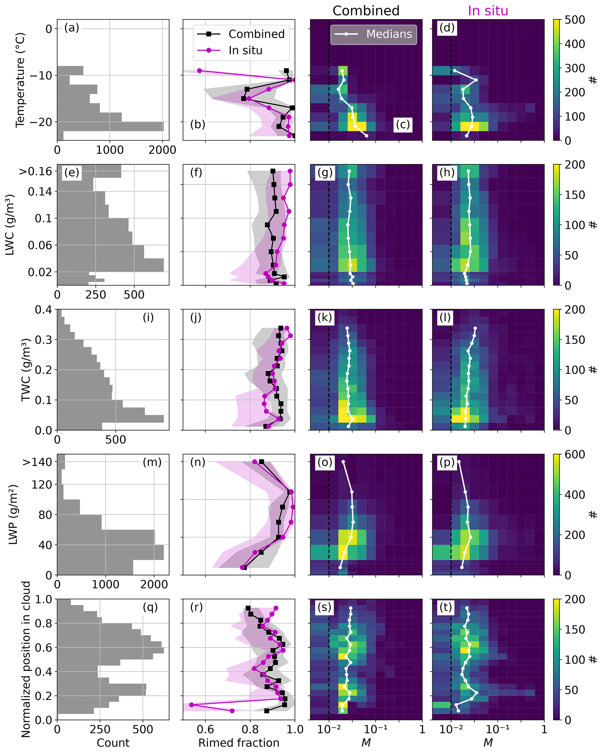
Figure 9 Occurrence of riming during collocated flight segments derived with combined (black) and in situ methods (magenta) depending on (a–d) Polar 6 noseboom temperature (in °C), (e–h) Nevzorov-probe-measured LWC (in g m⁻³), (i–l) Nevzorov-probe-measured TWC (in g m⁻³), (m–p) MiRAC-A-retrieved LWP (in g m⁻²), and (q–t) normalized position of Polar 6 in-cloud (0 meaning bottom of cloud, 1 meaning top of cloud). Bin sizes are 2 K, 0.02 g m⁻³ (0.005 g m⁻³ below 0.02 g m⁻³), 0.025 g m⁻³, 20 g m⁻², and 0.05, respectively. The first column shows the number of data per bin. The second column shows the rimed fraction, assuming M<0.01 to be unrimed, derived with combined (black squares) and in situ methods (magenta circles). Uncertainty estimates are shaded (combined: OE standard deviation, in situ: 30 s running standard deviation). The third and fourth columns show 2D histograms of M results for combined and in situ methods, respectively, including medians for each bin in white. The dashed black line shows M=0.01. All values with M<0.01 are grouped together in the lowest bin. Medians and average rimed fractions are only shown when there are more than 100 data points per bin. Nevzorov probe data are only available in April.

When analyzing the relation of riming to temperature, moderate riming also occurs at low temperatures below −15 °C. Between −10 and −15 °C, (local) minima of rimed fractions and M are evident with both methods. This coincides with the so-called dendritic growth zone, where aggregation is favored (Takahashi et al., 1991; Takahashi, 2014). Complex aggregated forms can appear to be round when viewed from certain angles and imaged with a limited resolution. This might lead to an overestimation of riming with the in situ method. Note that the temperature is available only at the point of observation, not where – at potentially colder temperatures – the riming process itself took place. The disagreement above −10 °C stems from a 10 min flight segment on 4 April, where M results from the in situ method go slightly below 0.01, while M results from the combined method stay slightly above 0.01. Median (25 %–75 % quantile range) M values are 0.019 (0.016–0.020) and 0.012 (0.006–0.016) for the combined and in situ methods, respectively.

There is no clear dependence of riming on LWC. The rimed particles could easily have undergone riming in an SLW layer above and fallen out to a place in the cloud with little to no SLW. Rimed fraction only increases slightly with TWC. This is likely because M results are low for the whole campaign, and large, unrimed aggregates can also result in large TWC.

For LWP, median M and rimed fractions increase with increasing LWP up until 50 g m⁻² and decrease in the two highest LWP bins. This decrease could be due to limited sampling as the bins contain less than 500 data points. Overall, the agreement between both methods is very good, with rimed fractions agreeing, on average, within 3 percentage points below and 11 percentage points above 100 g m⁻².

Rimed fractions agree within 2.7 percentage points for in-cloud positions above 0.2 (meaning Polar 6 is flying higher than the lowest 20 % of the cloud). Below 0.2, rimed fractions derived by the in situ method are, on average, 19.5 percentage points lower than those derived by the combined method. However, median M values agree within a factor 0.29 above and 0.17 below 0.2. Because our definition of a cloud includes precipitation below, low cloud positions might be below the liquid cloud base. If this is indeed the case, we expect the falling particles to be larger and heavier than the particles in the cloud above. The detection efficiency of cloud probes is worse for particles close to the upper end of their size range, even if we count particles that touch edges (as is done in the PSD calculation). Therefore the higher rimed fractions obtained by the combined method could be due to missing large particles in the PSD that the radar can see. The optimal estimation retrieval would then overcompensate by increasing M, resulting in a higher number of rimed particle populations for the combined method. Averaging the in situ data for longer time spans should ensure the capture of more large particles. Using running averages of 60 instead of 30 s shifts the rimed fractions below 0.2 only slightly closer together (agreement within 18.8 percent points; not shown). However, average particle sizes increase at small normalized positions in-cloud. Median values of D₃₂ increase by about 150 % from 1.52 mm at 0.15–0.2 to 3.71 mm at 0.05–0.1. Disagreement between both methods is higher when Polar 6 is flying near the top of the radar signal (Fig. D1) due to the higher variability of measurements, as we show in Appendix D.

4.4 In-situ-only flights

Here, we extend the analysis to periods only covered by the in situ aircraft to analyze how representative of the complete Polar 6 data the collocated measurements are. Even though a large, unique data set of collocated, airborne measurements was collected in the Arctic during HALO-(AC)³, the total amount of in situ cloud measurement time exceeds the collocated measurement time by a factor of 5. Figure 10 shows the dependence of M on temperature and LWC as in Fig. 9 but for the extended in situ data set. The position of Polar 6 in-cloud and MiRAC-A-retrieved LWP must be omitted due to the missing Polar 5 remote sensing information. TWC is not shown due to not adding further information, as discussed in Sect. 4.3. The average rimed fraction, assuming M<0.01 (M<0.05) to be unrimed, is 69 % (13 %), with a mean M=0.030, median M=0.016, and a 25 % to 75 % quantile range of 0.009 to 0.031. These values are slightly lower and indicate a slight shift towards more riming during the collocated segments.

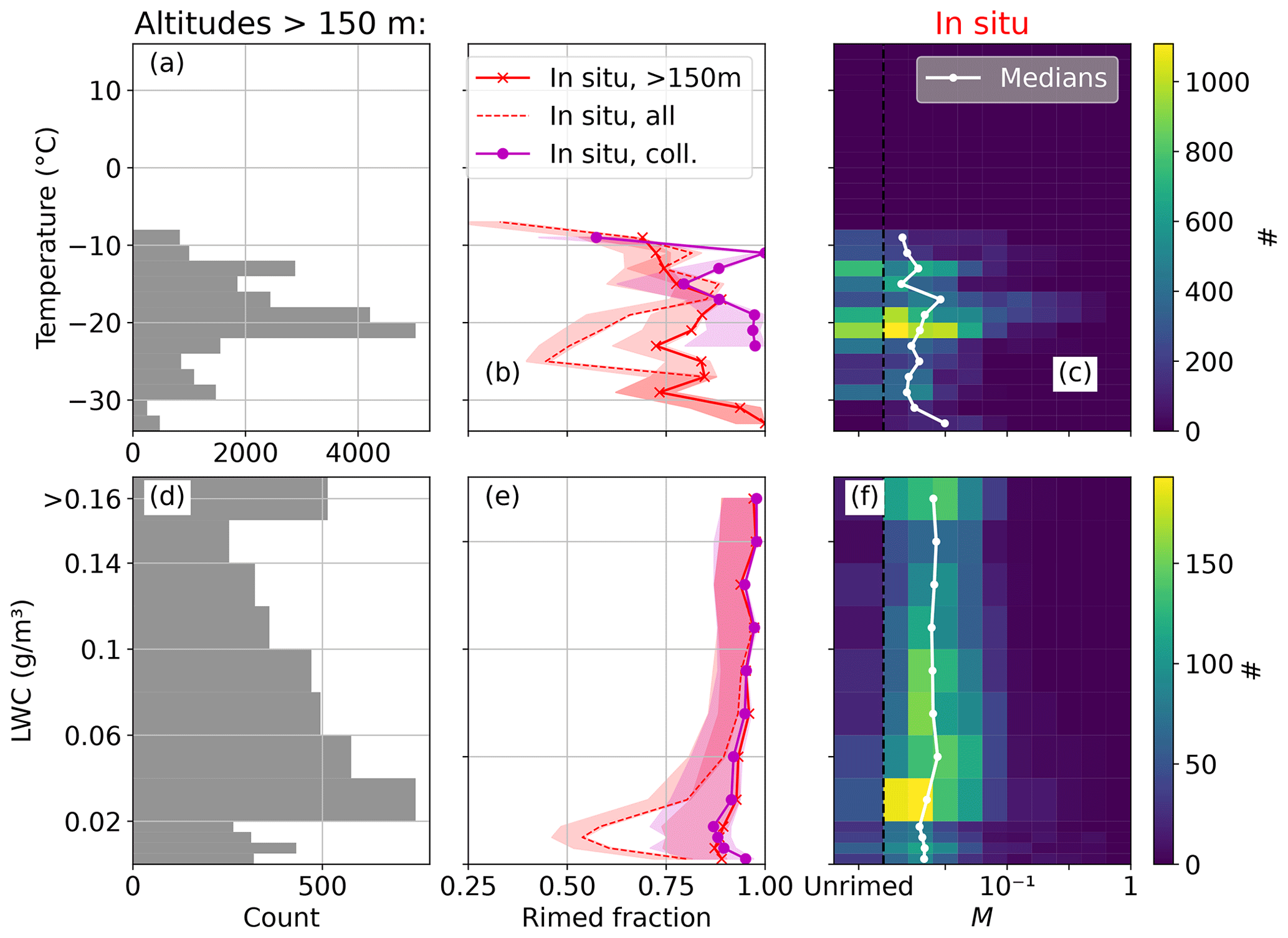
Figure 10 As in Fig. 9a–h but only for the in situ method for all Polar 6 flights with altitudes above 150 m. Rimed fractions for all flight segments are shown as red crosses, whereas results for collocated flights are repeated as magenta circles in (b) and (e). All data including flight altitudes below 150 m are shown as dashed red lines. Nevzorov probe data are only available in April.

When focusing on temperature bins with a sufficiently high number of observations, we observed decreasing riming with decreasing temperature from −10 and −16 °C (Fig. 10b). The rimed fraction for all in situ flights follows a similar shape to the collocated sub-sample in that temperature range, albeit with a lower local maximum at −11 °C (0.72 vs. 1.0). There is a slight local minimum of median M and rimed fraction at about −14 °C. Lower rimed fractions and median M result for lower temperatures when including all Polar 6 data. Similarly, rimed fraction and median M are lower for LWC below 0.05 g m⁻³.

Differences between the in situ method results for only collocated vs. for all segments are smaller when excluding Polar 6 data below 150 m, as can be seen in Fig. 10: the rimed fraction curve is shifted towards larger values. Also, both rimed fraction vs. LWC curves are very close, deviating by a maximum of 5.4 percentage points. The better agreement above 150 m could be simply due to the higher proportion of common data points because the collocated M of the in situ method is a subset of the M of the in situ method derived for all Polar 6 flight segments. Another explanation could be the influence of cloudless ice crystal precipitation (diamond dust). This phenomenon describes the formation of ice crystals under clear or nearly clear skies. Diamond dust typically occurs between November and mid-May at heights below 250 m over the Arctic Ocean (Intrieri and Shupe, 2004). This could shift the curve towards less riming for cold temperatures, resulting in a (near-) disappearance of the −15 °C local minimum.

We can conclude that the collocated flight segments are, in part, representative of all Polar 6 flight segments where Polar 6 flew above 150 m: they show similar behavior in terms of M dependence on LWC. However the collocated segments are biased towards higher amounts of rimed particles at low temperatures below −17 °C.

5 Conclusions

In this study, we present two methods to quantify riming with the normalized rime mass M using airborne in situ and remote sensing observations. We apply both methods to data collected during the HALO-(AC)³ field campaign performed in March–April 2022. One objective of HALO-(AC)³ was performing collocated flights with up to three aircraft. We focus on the research aircraft Polar 5 and Polar 6, which collected closely spatially collocated and almost simultaneous in situ and remote sensing observations west of Svalbard.

The first method takes advantage of these collocated flight segments to derive M. We developed an optimal estimation algorithm to retrieve M from a combination of radar and in situ measurements by matching measured with simulated radar reflectivities Z_e obtained from observed in situ particle number concentrations. As forward operator, we use the Passive and Active Microwave radiative TRAnsfer tool (PAMTRA), which includes empirical relationships of M and particle properties from Maherndl et al. (2023a) for estimating particle-scattering properties. The latter are obtained via aggregation and riming model calculations.

With the second method, M can be derived from in-situ-measured particle shape alone. We calculated the complexity χ of in-situ-measured particles, which relates particle perimeter to area. Further, we derived M from empirical relationships that were again obtained from synthetic particles. However, we find that this method is only reliable when sufficient numbers of particles large enough to calculate meaningful χ are detected with the in situ probes. A threshold of seven particles per second appears to result in a good performance.

We compare the obtained M derived by both methods: combined and in situ methods result in median (mean) M of 0.024 (0.035) and 0.021 (0.033) during collocated segments, and M distributions look remarkably similar. However, data-point-per-data-point agreement could not be achieved for all flight segments. Looking at each flight with collocation individually, we find similar results, except for 10 April, when the combined method shows higher M than the in situ method. By visual inspection of CIP and PIP images for the 6 min of collocated measurements, we find the higher M predicted by the combined method to be closer to the truth. Likely, the in situ method performs worse because a significant number of rimed particles fall into the size range that cannot be used; i.e., particles are too large for the CIP but too small to derive χ from PIP.

Using a case study, we show that we achieve good agreement in terms of temporal confluctuations as long as measurements are homogeneous, which is more often the case when Polar 6 is flying deeper in-cloud. Under inhomogeneous conditions, both methods agree in a statistical sense. M appears to increase and decrease periodically in correspondence with Z_e, indicating that riming plays an important role in the Z_e variability, which is commonly observed in Arctic MPCs.

In addition, we analyzed the dependence of M on air temperature, LWC, LWP, and the position of Polar 6 in the cloud. Rimed fractions (assuming M<0.01 to be unrimed) agree, on average, within 7 percentage points. With either method, we do not find a clear relation between LWC and riming during the collocated segments. LWP shows a positive correlation with riming below 130 g m⁻². We confirm findings from Fitch and Garrett (2022), which show that riming also occurs in Arctic clouds with low LWP. Both methods show a decrease in riming at about −15 °C, which corresponds to the dendritic growth zone (Takahashi et al., 1991; Takahashi, 2014). When extending the in situ method to all Polar 6 flights, these findings hold as long as low flight segments are excluded. Close to the upper edge of the radar signal (cloud top as seen by the radar reflectivity measurements), the methods disagree, especially when comparing data point per data point. The combined method shows higher rimed fractions and M than the in situ method (Fig. D1). We think that this is likely due to the higher variability of cloud properties at cloud top resulting in less tolerance of the results compared to the collocation of Polar 5 and Polar 6. Disagreement is also larger close to cloud bottom, which includes precipitation below the cloud, due to detection of the liquid cloud base being unavailable from the aircraft measurements. We think that large particles that are missed by the cloud probes due to detection efficiency but seen by the radar might be the reason for higher riming fractions from the combined method. Median values of D₃₂ over all collocated segments increase by about 150 % from 1.52 mm at a normalized position in-cloud of 0.15–0.2 to 3.71 mm at 0.05–0.1.

With both methods, we derive average M over the particle population observed at a given time step. However, we often observed mixtures of pristine and rimed particles of different sizes during the campaign. While we correct the in situ method M, accounting for the size-dependent detection efficiency of CIP and PIP, we are still left with a size gap between probes. M results obtained with the in situ method are therefore biased towards particles smaller than 1 mm and particles larger than 1.4 mm. Because Z_e is more sensitive to large particles, M derived by the combined method is likely skewed towards the right tail of the PSD. In future studies, the in situ method can be adapted to derive size distributions of M (given the particle count per bin is sufficiently large) to compensate for this. Additionally, implementing a particle type identification algorithm will likely improve the uncertainties of both methods and should be investigated in future studies.

The presented methods provide tools to better quantify riming in MPCs from airborne observations. This allows us to study external drivers and the variability of riming.

Appendix A: Assumption on particle shape

For both the combined and in situ methods, we assume the particle shape to be dendrites. Here we show results assuming plates or columns and discuss implications for our results. We chose to show M plots in linear scale due to the larger uncertainties at high M values.

Figure A1 shows M results for the combined method using the mass size parameter for plates and columns from Maherndl et al. (2023a). We do not show rosettes or needles because the temperature range observed during HALO-(AC)³ does not favor these ice particle shapes (needles commonly occur at −5 °C and warmer, and rosettes occur at −40 °C and colder). While M results for columns are lower than for dendrites (Fig. A1a), plates and dendrites result in the same M within the uncertainty estimates (Fig. A1b). Although we expect the majority of data to be collected in a plate-like growth regime (92 % of collocated and 81 % of total in situ cloud data were collected in a temperature range of −10 to −30 °C (excluding 10 April)), the lower M results for columns could explain the discrepancy between both methods at temperatures warmer than −10 °C (Fig. 9b).

Similarly, Fig. A2 shows M results of the in situ method using plates and columns to derive fit coefficients. Within uncertainty estimates, which are derived from the standard deviations over the 30 s averaging window, M results for columns and plates agree with those for dendrites. Still, we want to note that there is a positive bias for M derived for dendrites compared to plates and a negative bias compared to columns. This could further explain the discrepancy between combined and in situ methods at temperatures above −10 °C.

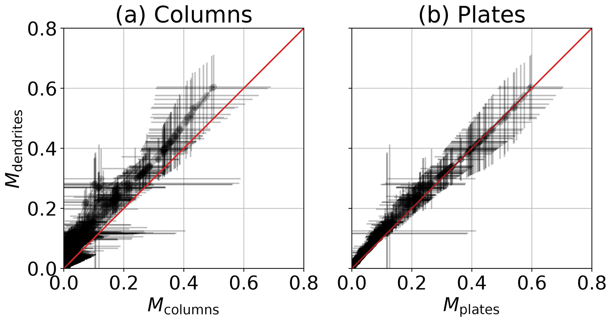
Figure A1 OE retrieval (combined method) results assuming mass size parameters for (a) columns M_columns and (b) plates M_plates. The 1 : 1 line is shown in red.

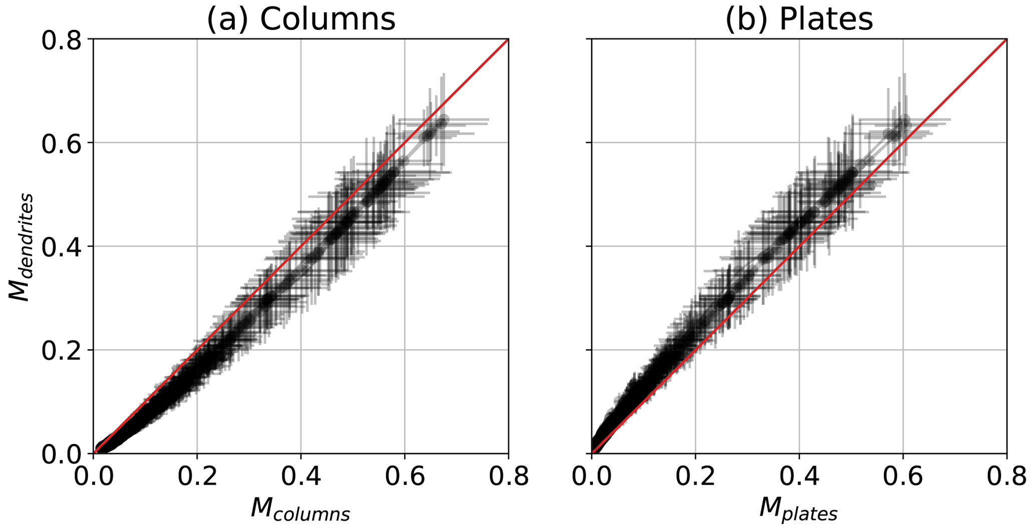
Figure A2 In situ method results assuming (a) columns M_columns and (b) plates M_plates. The 1 : 1 line is shown in red.

As described in Sect. 3.2, we use simulated rimed aggregates from Maherndl et al. (2023a) to derive empirical relations. For columns and plates, the following functions result (with R² = 0.92 and 0.93, respectively; D_max is again in pixels):

$$\begin{array}{}\text{(A1)}& {\displaystyle }{\log }_{\mathrm{10}}\left(M_{\mathrm{columns}}\right)={\displaystyle \frac{\mathrm{1.33}-\mathit{\chi }+\mathrm{0.0000903}\cdot D_{\max }}{\mathrm{0.00291}\cdot D_{\max }+\mathrm{0.115}}},\text{(A2)}& {\displaystyle }{\log }_{\mathrm{10}}\left(M_{\mathrm{plates}}\right)={\displaystyle \frac{\mathrm{1.33}-\mathit{\chi }+\mathrm{0.000223}\cdot D_{\max }}{\mathrm{0.00291}\cdot D_{\max }+\mathrm{0.0370}}}.\end{array}$$

Appendix B: Validation of the combined method with synthetic data

To approximate errors of the combined method M retrieval, we present results obtained for synthetic data. We use the simulated rimed dendrite aggregates from Maherndl et al. (2023a) binned into 10 logarithmic M bins from 10⁻² to 10⁰ (“true” M) and linear D_max bins from 0 to 10 mm with bin widths of 200 µm. We apply exponential PSDs $N\left(D\right)=N_{\mathrm{0}}\exp (-\mathrm{\Lambda }D)$ to each M bin, where N is the number concentration (in m⁻⁴) of particles of size D (in m), the intercept parameter N₀ (in m⁻⁴) describes the overall scaling, and the slope parameter Λ controls the shape. Similarly to Maherndl et al. (2023a), we derive N₀ with the empirical function from Field et al. (2006) for temperatures T from −25 to −1 °C in 1 K steps. We calculate Λ from the total number of particles N_tot with $\mathrm{\Lambda }=N_{\mathrm{0}}/N_{\mathrm{tot}}$ m⁻¹ and vary N_tot from 500 to 4500 m⁻³ in 500 m⁻³ steps. This results in a total of 2250 PSDs. We use PAMTRA to calculate Z_e from the PSDs with the same setup as for the observations (see Sect. 3.1). We use the exact particle masses from the aggregation and riming model results and the SSRGA parameter calculated with snowScatt (Ori et al., 2021) that was used as a reference in Maherndl et al. (2023a). The resulting Z_e values are assumed to be the truth and are referred to as Z_e,true.

We then apply the retrieval framework of the combined method using the generated PSD in the forward operator F and Z_e,true as y. To be consistent, we assume ${\mathit{x}}_{\mathrm{a}}=-\mathrm{1}$ (corresponding to M=0.1) to be a priori information, S_a=1 to be a priori uncertainty, and S_y to correspond to a measurement uncertainty of 1.5 dB. Mass–size and scattering are parameterized with the riming-dependent parameterization (Maherndl et al., 2023a). We therefore treat the synthetic data analogously to the in situ observations and pretend that the mass of the particles is unknown.

Figure B1 shows (a) the resulting Z_e derived with the OE framework plotted against Z_e,true and (b) the retrieved M plotted against the true M. OE Z_e has a mean bias of −0.05 dB and an absolute mean bias of 0.09 dB compared to Z_e,true; both are well within the assumed measurement uncertainties. M is overestimated slightly for low M_true. This stems from the slight positive bias of less than 1 dB of the riming-dependent parameterization for lightly rimed particles when applying exponential sizes (see Fig. 10b of Maherndl et al., 2023a). In logarithmic space, the M results have a mean bias of 7.7 %, which corresponds to 20 % in linear space. The uncertainty output from the OE estimation scheme results in a state space variance S_x, corresponding to an M uncertainty of 7.8 % (in the logarithmic framework).

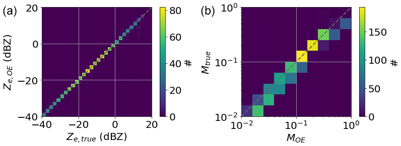
Figure B1 OE retrieval (combined method) results with synthetic data: (a) reflectivity Z_e,OE vs. reflectivity Z_e,true calculated with exact particle masses and snowScatt-derived SSRGA parameters; (b) retrieved M_OE vs. true M_true.

Appendix C: In situ method weighting factors

Table C1 shows the weighing factors that were derived for CIP and PIP by comparing counts of all particles to particles that do not touch the edges of the OAPs.

Table C1 Weighting factors w_CIP and w_PIP that were derived to account for the size-dependent detection efficiency of the probes.

Appendix D: Limitations close to radar signal cloud top

Near the top edge of the measured radar signal, disagreement between the in situ and combined methods is higher (Fig. D1), which could be due to higher variability of cloud properties there: while the radar on board Polar 5 might see a gap in clouds, Polar 6 might fly a few hundred meters away in a cloudy region. Alternatively, the radar could see signatures of clouds due to its larger footprint, while the cloud probes on Polar 6 measured no particles in close proximity. Both cases do not (or rarely) occur when Polar 6 is further in the cloud, where cloud properties are more homogeneous. The in situ method could also be less reliable at cloud top due to lower sample sizes. Given the available data, a concluding explanation cannot be given.

Figure D1 As in Fig. 9r–t but for the position of Polar 6 in the radar signal, with 0 meaning cloud bottom as seen by radar (minimum 150 m due to surface clutter) and 1 meaning cloud top as seen by radar.