Lidar depolarization characterization using a reference system

In this study, we present a new approach for the determination of polarization parameters of the Nicosia Cimel CE376 lidar system, using the Polly^XT in Limassol as a reference instrument. The method is applied retrospectively to the measurements obtained during the 2021 Cyprus Fall Campaign. Lidar depolarization measurements represent valuable information for aerosol typing and for the quantification of some specific aerosol types such as dust and volcanic ash. An accurate characterization is required for quality measurements and to remove instrumental artifacts. In this article, we use the Polly^XT, a widely used depolarization lidar, as our reference to evaluate the CE376 system's gain ratio and channel cross-talk. We use observations of transported dust from desert regions for this approach, with layers in the free troposphere. Above the boundary layer and the highest terrain elevation of the region, we can expect that, for long-range transport of aerosols, local effects should not affect the aerosol mixture enough for us to expect similar depolarization properties at the two stations (separated by ∼ 60 km). Algebraic equations are used to derive polarization parameters from the comparison of the volume depolarization ratio measured by the two systems. The applied methodology offers a promising opportunity to evaluate the polarization parameters of a lidar system, in cases where a priori knowledge of the cross-talk parameters is not available, or to transfer the polarization parameters from one system to the other.

1 Introduction

Understanding the aerosol vertical stratification can help in reducing the uncertainties related to aerosol radiative forcings which remain large (IPCC, 2021). For more accurate estimations, it is essential to improve the knowledge of the aerosol characteristics: shape, size, and optical properties. The diversity of combinations of aerosol sources and transport mechanisms leads to the high variability of the distribution of aerosols with different characteristics, which makes their classification a complicated task (Di Iorio et al., 2003).

Lidar has become a widely used tool for studying highly resolved information on the spatial and temporal distribution of aerosols. On this, several key campaigns, such as SAMUM–1, SAMUM–2 (Groß et al., 2011; Tesche et al., 2011), and the ASKOS experiment (Marinou et al., 2023), were performed, and they successfully demonstrate the capabilities of lidar systems. These were not the first to demonstrate aerosol lidars: earlier works include those of Reagan et al. (1977), Brogniez et al. (1992), and Krueger (1993). In contrast to traditional setups with in situ or airborne sensors, like optical particle counters (OPCs) or particle sizers (Di Girolamo et al., 2022), lidars (ground- or satellite-based) can provide information on the temporal variability and on the vertical structure up to the stratosphere. In addition, they provide insights on aerosol size and optical properties.

Cyprus, situated between large deserts, is actively involved in advancing atmospheric science and aerosol research. The region's unique location has made it an invaluable site for diverse studies on dust, among other aerosol types (e.g., detection of Canadian wildfire smoke over Cyprus; Baars et al., 2019). For example, Mamouri and Nisantzi's work (Mamouri et al., 2013; Mamouri and Ansmann, 2014; Mamouri et al., 2016; Mamouri and Ansmann, 2016; Nisantzi et al., 2014, 2015) introduced novel methodologies for dust profiling using polarization lidar, analyzing dust outbreaks over Cyprus. Nisantzi et al. (2014, 2015) explored lofted fire smoke plumes' mineral dust content and compared extinction ratios for desert dust in Cyprus. Mamouri et al. (2016) comprehensively detailed extreme dust storms in the Cyprus region, showcasing EARLINET observations. Additionally, studies by Kezoudi et al. (2021) and Mamali et al. (2018) compared UAV-based OPC observations with lidar, enriching knowledge on Saharan dust over Cyprus. Moreover, the key campaigns CyCARE and A-LIFE had strong contributions by depolarization lidar and aimed to investigate properties of complex aerosol mixtures often observed over the island of Cyprus (Ansmann et al., 2019; Floutsi et al., 2023). These collective efforts highlight Cyprus's significant contributions to the understanding of aerosol properties.

The contribution of lidar to greater science is undoubtedly important as it is a fundamental tool for monitoring anthropogenic and natural aerosols. Sand and dust storms, or volcanic ash transport in the case of volcanic eruptions, can impact human health and everyday life. The WMO's Sand and Dust Storm Warning Advisory and Assessment System (SDS-WAS) benefits from available lidar networks (e.g., EARLINET; Schneider et al., 2000) for the monitoring of vertical profiles of winds and aerosols (Basart et al., 2019). Similarly, lidars installed across different locations aim to improve detection and aid forecasting of volcanic ash in the event of future eruptions by providing observations to local Volcanic Ash Advisory Centers (VAACs) (Sassen et al., 2007; Osborne et al., 2022).

The addition of a depolarization channel on a lidar system offers the capability to discriminate between different types of atmospheric particles, for example, low-depolarizing urban aerosols and high-depolarizing dust aerosols or liquid and ice clouds. Discriminating between liquid and ice water can provide a better understanding of the aerosol–cloud interactions (e.g., Seifert et al., 2010). Aerosols can change the properties of clouds, therefore affecting indirectly their radiative forcing (Senior and Mitchell, 1993; Fowler and Randall, 2002). Aerosol typing can be quite complex when the observed atmospheric layers consist of multiple aerosol types.

Lidar depolarization measurements represent an excellent method to detect and quantify some specific aerosol types such as dust and volcanic ash (Cairo et al., 1999; Tesche et al., 2009; Freudenthaler et al., 2009). Using this information, several studies aim to describe the properties and temporal evolution of each of the aerosol layers types (Hoffmann et al., 2010; Ansmann et al., 2011; Marenco and Hogan, 2011). They also permit the distinction between ice crystals and water droplets (Ansmann et al., 2005) and the discrimination of types of polar stratospheric clouds (Toon et al., 2000). The depolarization lidar technique is simple and reliable and is not as limited by daylight background as in the case of acquiring Raman signals.

Spherical particles in the atmosphere have no depolarization for 180° backscattering (Van de Hulst, 1957); hence, a depolarization signal is an indication of non-sphericity such as in ice crystals or irregularly shaped aerosols. Most lidar systems use linearly polarized lasers (linear depolarization measurements), and such systems are used also in this paper. Some circular polarization lidar systems exist, such as the Enhancement and Validation of ESA products (eVe), which provide useful information for layers with oriented particles and where multiple scattering cannot be neglected (Paschou et al., 2022).

The volume linear depolarization ratio (VLDR), or simply volume depolarization ratio (VDR), is usually defined as the ratio between the atmospheric cross sections for cross-polarized and co-polarized backscattering and is a measure of the overall properties of the atmospheric volume, comprising a mixture of molecules and particles. This is typically measured by means of a polarizing beamsplitter (PBS) in the receiving system and by taking the ratio of signals in the two channels. In reality, the measurement is more complex than this, and it requires accounting for the gain ratio of the channels and for the cross-talk between them: this is what we refer to here as the determination of the lidar polarization parameters. If this step is not achieved correctly, systematic errors appear with a significant impact.

Addressing instrumental effects on depolarization channels is pivotal, as numerous optical components within lidar systems can introduce substantial systematic errors in atmospheric depolarization values. Freudenthaler (2016) introduced analytical equations to assess the dependence of lidar signals on polarization parameters and different calibration setups. Both Bravo-Aranda et al. (2016) and Belegante et al. (2018) emphasize that systematic errors can be significant if the lidar system is not well characterized and aligned, underscoring the need for careful consideration of optical components. Well-characterized VDR measurements permit, on the one hand, reconstruction of the total lidar signal by the recombination of the two channels: this is needed for the retrieval of the particle backscattering and extinction coefficients. On the other hand, they permit the computation of the particle linear depolarization ratio (PLDR), or simply particle depolarization ratio (PDR), which abstracts from the influence of air molecules and is hence an intrinsic property of the particles (Freudenthaler et al., 2009). In a well-characterized lidar system for depolarization, the channel gain ratio and all the elements contributing to an imperfect separation of the depolarization channels in the hardware are well known. The latter includes the polarizing beamsplitter transmittances and reflectances for the co-polar and cross-polar beams, as well as the laser polarization purity and its rotation angle compared to the frame of reference of the receiver (Freudenthaler et al., 2009; Freudenthaler, 2016). In particular, the laser rotation angle ϕ is not easily known, and an additional experimental apparatus has been used in a few papers in order to quantify it (Alvarez et al., 2006; Belegante et al., 2018; Osborne, 2022). The additional apparatus consists of a rotatable half-wave plate (HWP) added in front of the receiver optical path, and a calibration sequence has to be performed where atmospheric measurements are acquired by artificially varying the system’s cross-talk through the rotation of the half-wave plate.

At the Cyprus Institute (CYI), we have recently acquired a new compact Cimel CE376 lidar system, which we have operated continuously in Nicosia, Cyprus, since September 2021. This is a low-power and compact two-wavelength lidar system, ideal for campaigns and mobile observations, able to operate in all weather conditions, and able to detect the molecular signal up to 10 km in the daytime and 18 km in the nighttime with a good signal-to-noise (SNR) ratio. We have, however, found an issue in the initial depolarization calibration related to the observed VDR of purely molecular layers, which is too high compared to the expected value computed according to Behrendt and Nakamura (2002). Whereas a technological solution is planned with Cimel in the near future, this paper is about a method for correcting past data by correlating the lidar measurements to a reference-calibrated lidar system, also located on the island, which for this paper we consider to be our reference system. This will be called the atmospheric characterization approach to the lidar polarization parameters.

In Sect. 2, we present the depolarization lidar equations to be used for the depolarization characterization. Then, in Sect. 3, we describe the systems used in this study, focusing on the technical characteristics and locations. Section 4 presents the lidar depolarization characterization methodology, providing demonstration examples from past observations. Finally, Sect. 5 summarizes and concludes the main findings of the application of the discussed method.

2 Theoretical concept

In an ideal depolarization lidar, the range-corrected signal in the co-polar and cross-polar channels, P^∥ and P^⟂, can be expressed as follows, in the function of the atmospheric-volume cross sections β^∥ and β^⟂ for non-depolarizing and depolarizing backscattering, respectively:

$$\begin{array}{}\text{(1)}& {\displaystyle }{P}^{\parallel }\left(R\right)=K^{\parallel }T\left(R\right){\mathit{\beta }}^{\parallel }\left(R\right)\text{(2)}& {\displaystyle }{P}^{⟂}\left(R\right)=K^{⟂}T\left(R\right){\mathit{\beta }}^{⟂}\left(R\right),\end{array}$$

where R is the range, T(R) is the two-way atmospheric transmittance between ranges 0 and R, and K^∥ and K^⟂ are the lidar constants for both channels.

The VDR is defined as the ratio $\mathit{\delta }={\mathit{\beta }}^{⟂}/{\mathit{\beta }}^{\parallel }$. Note that cross-polarizing backscatter β^⟂ is unphysical and that other definitions of the VDR exist in the literature (see Gimmestad, 2008; Freudenthaler, 2016). However, the one used here has been commonly used in the legacy lidar literature (e.g., Freudenthaler et al., 2009). In the ideal case, the VDR is computed as

$$\begin{array}{}\text{(3)}& \mathit{\delta }={\displaystyle \frac{{\mathit{\delta }}^{\ast }}{K^{\ast }}},\end{array}$$

where ${\mathit{\delta }}^{\ast }=P^{⟂}/P^{\parallel }$ is the ratio of the two lidar signals (a sort of uncalibrated depolarization ratio) and $K^{\ast }=K^{⟂}/K^{\parallel }$ is the gain ratio between the two channels. For an ideal lidar, determining K^∗ is all that is needed to calibrate depolarization. Once this is done, the lidar range-corrected total signal, P, can be reconstructed as a signal proportional to ${\mathit{\beta }}^{\parallel }+{\mathit{\beta }}^{⟂}$. Hence,

$$\begin{array}{}\text{(4)}& P=P^{\parallel }+{\displaystyle \frac{P^{⟂}}{K^{\ast }}}.\end{array}$$

P(R) is what will be used in aerosol inversion schemes such as Fernald–Klett (Klett, 1985; Fernald, 1984) or Raman inversion (Ansmann et al., 1990, 1992a, b; Ferrare et al., 1998).

For a real depolarization lidar system, the equations need to account for the cross-talk between the two channels through the cross-talk constants, denoted as g and e in this paper, expressing, respectively, how much co-polar signal enters the cross-polar channel and vice versa, leading to the following expressions:

$$\begin{array}{}\text{(5)}& {\displaystyle }{P}^{\parallel }=K^{\parallel }T\left({\mathit{\beta }}^{\parallel }+e{\mathit{\beta }}^{⟂}\right)\text{(6)}& {\displaystyle }{P}^{⟂}=K^{⟂}T\left({\mathit{\beta }}^{⟂}+g{\mathit{\beta }}^{\parallel }\right).\end{array}$$

By dividing Eqs. (6) and (5) we derive δ^∗,

$$\begin{array}{}\text{(7)}& {\mathit{\delta }}^{\ast }=K^{\ast }{\displaystyle \frac{\mathit{\delta }+g}{\mathrm{1}+e\mathit{\delta }}},\end{array}$$

which can be resolved as follows:

$$\begin{array}{}\text{(8)}& \mathit{\delta }={\displaystyle \frac{{\mathit{\delta }}^{\ast }-K^{\ast }g}{K^{\ast }-e{\mathit{\delta }}^{\ast }}},\end{array}$$

and the total signal can be then calculated by

$$\begin{array}{}\text{(9)}& P=(\mathrm{1}-g)P^{\parallel }+(\mathrm{1}-e){\displaystyle \frac{P^{⟂}}{K^{\ast }}}.\end{array}$$

These full equations are going to be applied for the determination of the polarization parameters. In Freudenthaler et al. (2009) and Freudenthaler (2016), the approach is that they know their system well enough, including the various parameters contributing to errors in depolarization calibration, for calibration to only involve determining K^∗. In our case, we assume we do not know our system to this point, and we will retrieve these parameters from observations and a reference system (we call this the three-parameter depolarization characterization, since K^∗, g, and e are to be retrieved).

The effect of g will usually dominate in low-depolarization layers (e.g., particle-free or spherical-particle layers), so that we can attempt to simplify Eq. (8) by neglecting e:

$$\begin{array}{}\text{(10)}& \mathit{\delta }={\displaystyle \frac{{\mathit{\delta }}^{\ast }}{K^{\ast }}}-g,\end{array}$$

which can be summarized in a phrase by saying that, in addition to knowing the gain ratio K^∗, we must also know the “depolarization of the lidar system”, g (more precisely diattenuation), or alternatively that the depolarization equation involves a multiplicative and an additive parameter. Whereas it may not be the most correct way to neglect e for all lidar systems, this simplified equation has been used in the past for some systems: for example, it was used in Marenco and Hogan (2011, Eq. 5) and in Chazette et al. (2012, Eq. 6). We call the approach using this simplified equation the two-parameter depolarization characterization (given that only K^∗ and g can be determined). It must be noted that in high-depolarizing layers, the contribution of e is larger; therefore it should not be neglected (unless e≪1 for a particular system).

The following sections investigate these approaches and will highlight their advantages and drawbacks and compare their outcomes.

3 Instruments

3.1 Cimel lidar system

As was briefly introduced before, Cimel CE376 is a compact elastic backscatter lidar developed by Cimel in France (seen in Fig. 1a). It is a dual-wavelength polarization lidar equipped with a laser diode and frequency-doubled Nd:YAG laser, operating in the near-infrared (808 nm) and green (532 nm) with a repetition rate of 4.7 kHz. It has a small beam divergence (50 µrad) and field of view (120 µrad), making it suitable for aerosol profiling. It measures backscatter signals in three reception channels: one for the infrared and two for the green co-polar and cross-polar channels. The lidar uses photon-counting acquisition through avalanche photodiode detectors (SPCM-AQRH modules from Excelitas) for all the reception channels (schematic in Appendix E). The system has day and night operation with a typical detection altitude of around 10 km for the day and 18 km for the night. The signal is recorded in 2048 successive bins spaced by 15 m in the vertical direction from 100 m up to a range of 30 km. The integration time is 1 s. Before the raw Cimel lidar data can be used for the depolarization characterization method, they must be pre-processed to correct detection errors and remove ambient background signals on all three channels. The pre-processing that we apply consists of dead time, dark count, and background correction of the raw Cimel data. Furthermore, data are filtered for quality assurance based on applied thresholds on housekeeping parameters (relative humidity and temperature).

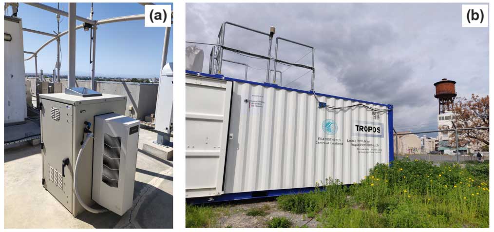
Figure 1 CE376 lidar with thermal enclosure on the roof of the premises of The Cyprus Institute in Nicosia (a) and Polly^XT container housing at CUT premises in Limassol (b).

The Cimel lidar was installed in September 2021 at the premises of The Cyprus Institute in Nicosia, Cyprus (35°8^′29.23^′′ N, 33°22^′51.49^′′ E) at 181 m above sea level (a.s.l.) and has been running continuously since. It was installed with a mechanical orientation directly to the vertical, ensuring vertical beam propagation with a precision of 1–2 µrad.

Nicosia is located in the center of the island between the largest mountain ranges of Cyprus: the Troodos Mountains, stretching across a third of the island and peaking at 1952 m, and the Kyrenia mountain range that runs along the northern coast of the island, peaking at 1024 m (see Fig. 2). The aerosol mixture above Nicosia is often a mixture of dust particles and anthropogenic haze.

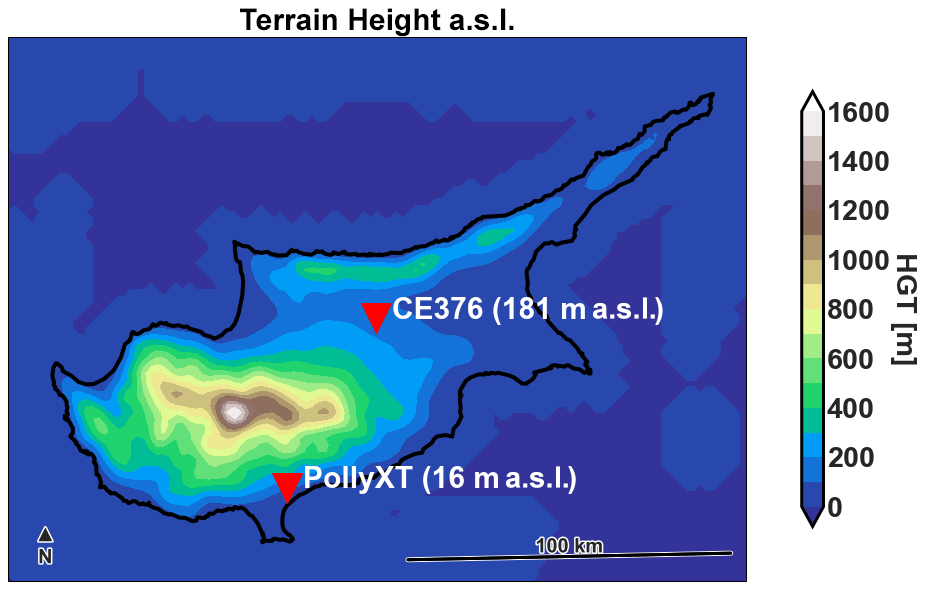
Figure 2 Cyprus topographic map. The red pins indicate the locations of Cimel CE376 in Nicosia and Polly^XT in Limassol.

The depolarization calibration suggested by the manufacturer follows the Δ(±45°) method described in Freudenthaler et al. (2009), later renamed to Δ(90°) (Freudenthaler, 2016). To rotate the plane of polarization a half-wave plate (HWP) is used in front of the polarizing beamsplitter cube. Note that a priori knowledge of the cross-talk parameters is required for this method; therefore, we use transmittances (T_p, T_s) provided by the polarizing beamsplitter (PBS) manufacturer (shown in Table 1) for the calibration constant (V^∗ in Freudenthaler et al., 2009, Eq. 10) calculations.

Table 1 Characteristic Δ(90°) PBS calibration coefficients (V^∗) and transmittances for the parallel and perpendicular polarizations (T_p and T_s).

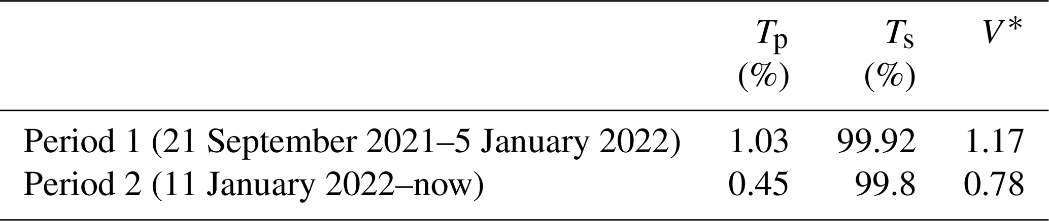
A depolarization calibration was performed during the installation of the lidar in order to derive the calibration coefficient V^∗ for the depolarization channel at 532 nm (found to be $V^{\ast }=\mathrm{1.17}$. $V^{\ast }\simeq K^{\ast }$; see Appendix A to understand the exact relationship between V^∗ and K^∗). However, the molecular depolarization at 5–5.5 km was measured to be ∼ 40 times larger than the computed molecular depolarization for the lidar characteristics. According to Behrendt and Nakamura (2002), for a narrow filter of 0.2 nm, which corresponds to the narrow filter of Cimel CE376, the computed molecular VDR is δ_m=0.0036. As this issue seemed to originate from the instrument and not the calibration, in January 2022, Cimel intervened on site to replace the PBS with a new one and repeated the calibration (giving a new $V^{\ast }=\mathrm{0.78}$). The PBS replacement did not suffice in improving the polarization measurements issue, which could be due to optical components inside the receiver and/or residual polarization from the laser. The intervention marks the conclusion of our first defined period and serves as the beginning of the second period, defined as periods 1 and 2 (dates seen in Table 1). Figure 3 summarizes these findings by comparing the computed molecular depolarization (δ_m) to two observed profiles on aerosol-free days from periods 1 and 2.

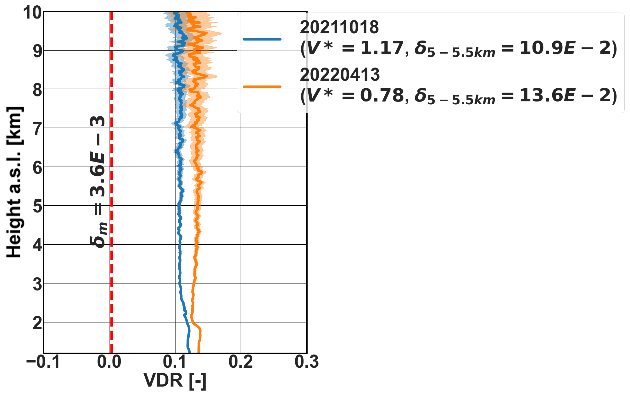
Figure 3 Measured volume depolarization with Cimel following Δ(90°) calibration for two cases dominated by molecular scattering above 3 km, with the case from period 1 in blue and the case from period 2 in orange. The dashed red line shows the computed depolarization ratio at molecular layers based on Behrendt and Nakamura (2002).

There are technical solutions that can be followed in order to improve the characterization of the system. Adding a motorized half-wave plate can reduce the human-induced uncertainty during the calibration procedure, but this would not resolve the cross-talk issue. Moreover, wire grid polarizers can be added to the PBS to reduce the cross-talk. The latter is planned for the near future but would not help to correct the depolarization measurements that were acquired so far. Such valuable measurements were obtained for more than 1 year in Nicosia, including the Fall Campaign that was performed in Cyprus in 2021. This research campaign was performed by the Cyprus Atmospheric Observatory (CAO; https://cao.cyi.ac.cy/, last access: December 2023) and the Unmanned Systems Research Laboratory (USRL; Kezoudi et al., 2021) of The Cyprus Institute (CYI), in collaboration with the Cyprus Atmospheric Remote Sensing Observatory (CARO) of the ERATOSTHENES Centre of Excellence (ECoE), with the aim of characterizing dust properties above the island (Kezoudi et al., 2022). During this campaign, measurements were obtained by remote sensing (lidars, ceilometers, and sun photometers) and UAV-based instrumentation (optical particle counters, backscatter sondes, and impactors able to collect dust samples). It is essential to have a method to characterize the depolarization for past data in order to make use of the Cimel lidar in synergy with the rest of the instrumentation, hence the motivation for this paper.

3.2 Polly^XT system

Polly^XT is a widely used instrument for aerosol observations which follows calibration and data quality assurance procedures according to EARLINET; hence it serves as our reference system in this paper. It was set up in October 2020 for continuous operation in Limassol, Cyprus (34°40^′36.01^′′ N, 33°2^′39.01^′′ E), at 11 m a.s.l. (location seen in Fig. 2), pointing at 5° off zenith to avoid specular reflections, and is part of PollyNET, a network of permanent or campaign-based Polly lidar stations (Baars et al., 2016). Polly^XT is a transportable aerosol multiwavelength Raman and polarization lidar that enables the determination of the particle backscatter coefficients at 355, 532, and 1064 nm and extinction coefficients at 355 and 532 nm. In addition, two depolarization channels at 532 and 355 nm are set up to differentiate between spherical and non-spherical aerosol particles from measurements of the PDR. Unlike the Cimel lidar, Polly^XT detects the total scatter light (all polarization planes) and the cross-polarized light. To characterize the depolarization, Polly^XT performs an automated Δ(90°) calibration twice per day (at 02:30 and 16:50 UTC). The calibration is automatically analyzed within the PollyNET processing chain (Baars et al., 2016; Yin and Baars, 2016). This type of lidar was previously introduced by Althausen et al. (2009) and Engelmann et al. (2016), whilst other publications presented the potential of these systems for monitoring aerosols in central Asia (Hofer et al., 2017, 2020a, b) and the southernmost region of South America (Jimenez et al., 2020).

Limassol is located on the other side of the Troodos mountain range with respect to Nicosia. Due to the topography, complex aerosol mixtures are observed over Limassol consisting of desert dust arriving from the Sahara or the Arabian desert; marine particles; urban pollution; and even smoke plumes, as shown in Mamouri and Nisantzi's work (Mamouri et al., 2013; Mamouri and Ansmann, 2014; Mamouri et al., 2016; Mamouri and Ansmann, 2016; Nisantzi et al., 2014, 2015).

In this paper, the systematic errors related to the volume linear depolarization ratio of the Polly^XT are taken from the study done by Bravo-Aranda et al. (2016), where the author provides some indications of the systematic errors based on the lidar model of Freudenthaler (2016). Based on that model, the systematic errors are Δδ(0.45)=0.0156 for dust layers and Δδ(0.004)=0.0057 for molecular range. The considered Polly^XT profiles of this paper are presented together with the aforementioned systematic error.

4 Lidar depolarization characterization

In this section, we describe the methodology on how to determine polarization parameters for the Cimel lidar using the Polly^XT as our reference system for selected cases during dust events for both periods 1 and 2, as seen in Table 1. For the atmospheric depolarization characterization, we selected cases with dust layers that were part of the long-distance advection of dust from nearby deserts. Dust over the island is considered to be fairly homogeneous in the free troposphere, and the distance between the Polly^XT and Cimel lidar is much smaller than the distance traveled from source regions. Ideally, an intercomparison should be done with both systems side by side to sample the same air mass. If this is not possible, for example, when already-existing data need to be corrected, someone has to select the cases carefully. For this paper, data were already available from the Cyprus Fall Campaign 2021, during which the two stations were separated by ∼ 60 km. Due to this spatial distance between the two lidars and the mountains in the area, the VDR could change because of atmospheric changes, e.g., temperature and relative humidity. In addition, it is recognized that pollution originating from northern African states might impact long-transported dust plumes. Studies, such as Groß et al. (2013), have demonstrated how this pollution can alter the lidar observations, mainly by reducing the depolarization ratio.

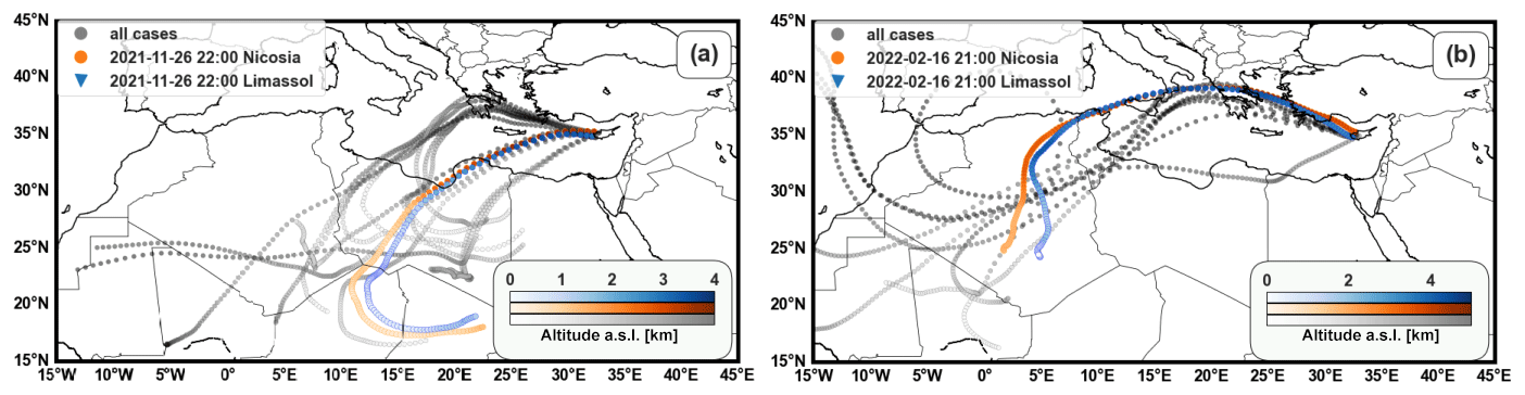
Figure 4 HYSPLIT back trajectories (https://www.ready.noaa.gov/, last access: December 2023) ending in Nicosia for all the selected cases for the first (a) and second (b) periods (the two periods are separated for illustration purposes). The two demonstration cases are highlighted for endpoints in Nicosia (orange) and Limassol (blue). Color scaling indicates the elevation of the layer, with lines getting darker as altitude increases. The arrival heights for 26 November 2021, 22:00 UTC, correspond to 3.3 km (Nicosia) and 3.1 km (Limassol), and for 16 February 2022, 21:00 UTC, the arrival heights are 4.1 km (Nicosia) and 3.9 km (Limassol). The arrival heights are chosen to be at the peak VDR of the dust layer.

Hence, it is important to carefully select the cases for which both lidars measure similar VDR profiles based on the following criteria: (i) dates with dust layers detected above 3 km, exceeding the topographic obstacle of the Troodos mountain range in the center of the island; (ii) molecular signal above the dust layer; (iii) selection of only nighttime profiles, to improve SNR; (iv) cloud-free scenes or high-level clouds only; and (v) general assessment of the meteorology to confirm the origin of air masses as being due to long-range transport. For all the cases used for the determination of polarization parameters, we have performed HYSPLIT (Stein et al., 2015) back trajectories (Fig. 4) to demonstrate that the air masses at arrival heights corresponding to the peak VDR values are produced over long distances and therefore are not affected by local effects. We believe that it is reasonable to neglect local differences for well-selected cases of free tropospheric layers having been transported from the same source region for more than 3000 km, given the short distance (60 km) between the two stations.

The method is based on some important assumptions. Firstly, we assume that the dust layer VDR is identical above 3 km in the profiles measured by the two systems. The second assumption is that there is no time shift between the two measurements. Only depolarization at 532 nm will be considered from the Polly^XT, which is the wavelength of the Cimel lidar depolarization measurements that we wish to characterize.

Before comparing the profiles from the two instruments, we apply time integration and smoothing on the CE376 and Polly^XT measurements to a common temporal and vertical range resolution (1 h and 82.5 m, respectively). The timestamps provided in this paper align with the starting moments of each 1 h interval. As a last step, we correct for the vertical shift observed in the profiles of the two lidars. This correction aims to remove the altitude difference between the two locations in the case of a sloping layer (more on this correction in Appendix C).

We demonstrate the proposed depolarization characterization approach using profiles from two nights that follow the criteria described before. As the dataset was limited (due to the selection criteria, i.e., dust layer above 3 km), the selected cases are taken from days with uniform dust layers over the island and for which the profiles of the two systems do not seem to be influenced by any local phenomena. The first profile corresponds to 26 November 2021, 22:00 UTC, and it is taken from a 5 d long dust event arriving from the Sahara (confirmed with HYSPLIT back trajectories; Fig. 4a), resulting in daily average AOD_500 nm values of 0.14 and 0.08 over Nicosia and Limassol, respectively (AERONET, https://aeronet.gsfc.nasa.gov, last access: December 2023). During this event, one uniform dust layer was observed from 2 to 4 km. The second profile corresponds to 16 February 2022, 21:00 UTC, and it is extracted from a relatively shorter event (2 d long) during which dust was also advected from the Sahara to Cyprus (Fig. 4b), but this time it was not as uniform in the vertical direction, with some distinct layers seen around 4 km. A cirrus cloud layer was also identified from 6 to 10 km. For the second event, the daily AOD_500 nm average over Nicosia was 0.20, whilst no data were available from Limassol's sun photometer. The VDR profile time series of the days from which we extracted the timestamps are seen in Fig. 5. From this figure we see how similar the VDR is at the high-depolarizing layers.

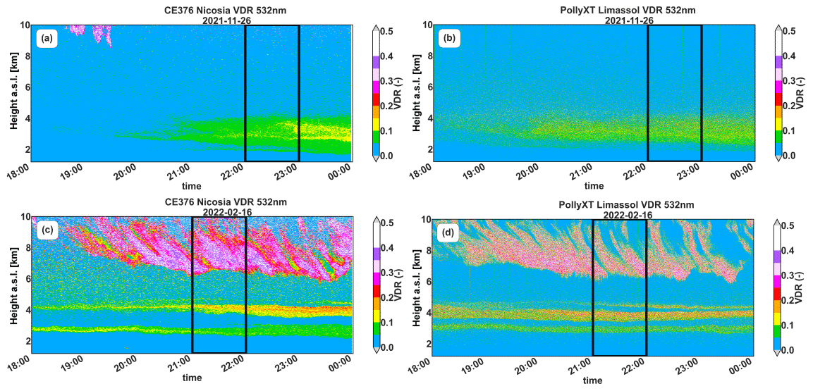
Figure 5 VDR observations by CE376 lidar in Nicosia and by Polly^XT in Limassol for 26 November 2021 (a, b) and 16 February 2022 (c, d) in 1 min time resolution. Panels (a) and (c) present the VDR from CE376 after the characterization of the polarization parameters using the two-parameter approach. Black lines indicate the 1 h average interval of the demonstrated cases.

4.1 Two-parameter depolarization characterization

In order to find the gain ratio K^∗ and cross-talk g, we create a system of equations following Eq. (10) using our reference measurements of the average volume depolarization ${\mathit{\delta }}_{\mathrm{d}}^{\mathrm{ref}}$ of a dust layer and the computed molecular depolarization, δ_m=0.0036, for the Cimel lidar, as mentioned also in Sect. 3.1. The calculation of the polarization parameters does not utilize signals from the reference lidar in the Rayleigh-scattering layers, as the VDR at these layers is instrument-dependent (depends on the receiver's bandwidth). Instead, we rely on the model of the molecular linear depolarization ratio by Behrendt and Nakamura (2002). For every examined profile, we select ${\mathit{\delta }}_{\mathrm{d}}^{\mathrm{ref}}$ from the reference instrument, and we select the channel signal ratio of dust (${\mathit{\delta }}_{\mathrm{d}}^{\ast }$) and of the molecular layer (${\mathit{\delta }}_{\mathrm{m}}^{\ast }$) from the Cimel instrument in the corresponding ranges. By applying Eq. (10) to these layers,

$$\begin{array}{}\text{(11)}& {\displaystyle }{\mathit{\delta }}_{\mathrm{ref}}^{\mathrm{d}}={\displaystyle \frac{{\mathit{\delta }}_{\mathrm{d}}^{\ast }}{K^{\ast }}}-g,\text{(12)}& {\displaystyle }{\mathit{\delta }}_{\mathrm{m}}={\displaystyle \frac{{\mathit{\delta }}_{\mathrm{m}}^{\ast }}{K^{\ast }}}-g,\end{array}$$

with two unknowns and two equations, we can solve for K^∗ and g:

$$\begin{array}{}\text{(13)}& {\displaystyle }{K}^{\ast }={\displaystyle \frac{{\mathit{\delta }}_{\mathrm{d}}^{\ast }-{\mathit{\delta }}_{\mathrm{m}}^{\ast }}{{\mathit{\delta }}_{\mathrm{ref}}^{\mathrm{d}}-{\mathit{\delta }}_{\mathrm{m}}}}\text{(14)}& {\displaystyle }g={\displaystyle \frac{{\mathit{\delta }}_{\mathrm{m}}^{\ast }{\mathit{\delta }}_{\mathrm{ref}}^{\mathrm{d}}-{\mathit{\delta }}_{\mathrm{d}}^{\ast }{\mathit{\delta }}_{\mathrm{m}}}{{\mathit{\delta }}_{\mathrm{d}}^{\ast }-{\mathit{\delta }}_{\mathrm{m}}^{\ast }}}.\end{array}$$

Figure 6 shows the application of the method described above for the cases considered in periods 1 and 2. In this figure, the resulting VDR profile (δ₂) is compared to the reference Polly^XT VDR profile (δ_ref) and the Cimel VDR profile (δ₁) calculated based on the Δ(90°) method described in Sect. 3.1. For the first case (26 November 2021, 22:00 UTC), ${\mathit{\delta }}_{\mathrm{ref}}^{\mathrm{d}}$ and ${\mathit{\delta }}_{\mathrm{d}}^{\ast }$ are selected in the range $h_{{\mathit{\delta }}_d}=\mathrm{3.1}$–3.4 km. The molecular range ${\mathit{\delta }}_{\mathrm{m}}^{\ast }$ for this case is chosen between $h_{{\mathit{\delta }}_{\mathrm{m}}^{\ast }}$ = 6–6.5 km. The VDR value at the molecular range after the correction is reduced from 0.158 ± 0.011 to 0.0033 ± 0.0067. In the dust layer, δ₂ = 0.0829± 0.0012 and δ_ref = 0.08319 ± 0.00087 compared to δ₁= 0.2840± 0.0019. The offset seen in the molecular VDR profile from the reference system is expected due to the unique interference filters of each instrument (the molecular VDR is strongly influenced by the instrument specification).

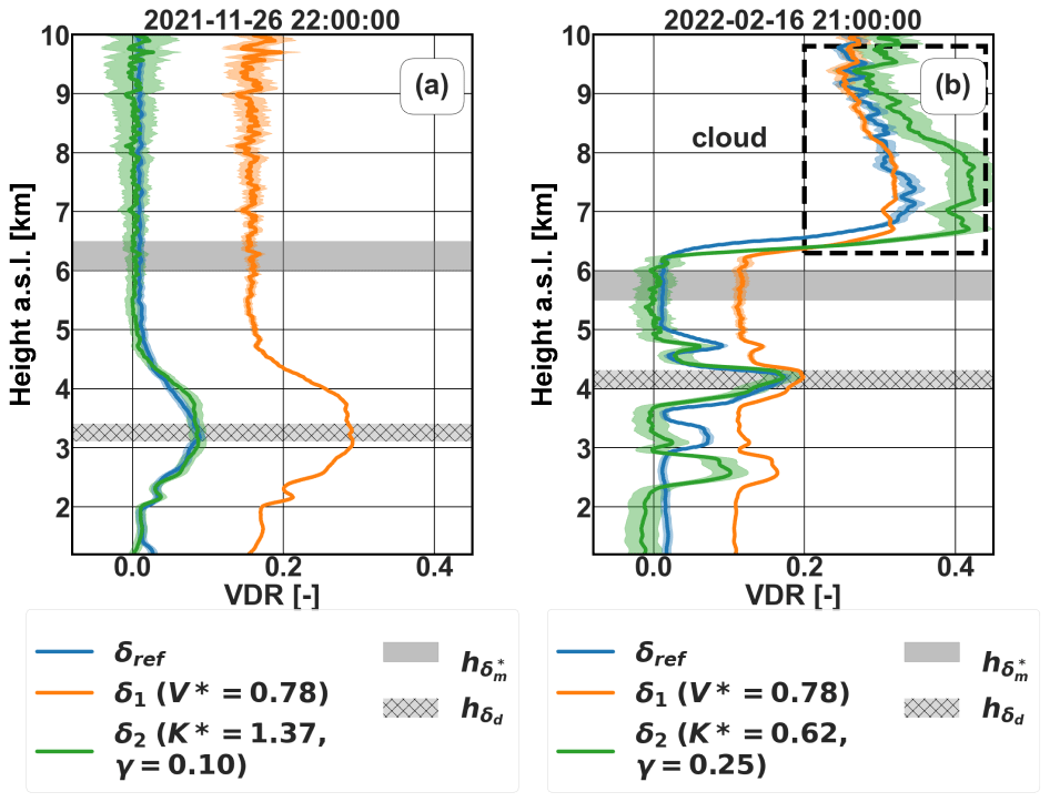
Figure 6 VDR profiles calculated using the two-parameter approach for (a) 26 November 2021, 22:00 UTC, corresponding to period 1, and (b) 16 February 2022, 21:00 UTC, corresponding to period 2, using the two-parameter approach. The non-corrected Cimel lidar VDR profile using the Δ(90°) calibration factors (δ₁) and the corrected profile (δ₂) using the two-parameter approach are compared to the reference Polly^XT lidar profile (δ_ref). The shaded regions indicate the reference ranges used for dust and molecular layers. Systematic errors of the reference instrument are shown in blue, and the statistical uncertainty of the Cimel profiles is shown in orange (non-corrected δ₁) and green (corrected δ₂).

For the second case (16 February 2022, 21:00 UTC), ${\mathit{\delta }}_{\mathrm{ref}}^{\mathrm{d}}$ and ${\mathit{\delta }}_{\mathrm{d}}^{\ast }$ are selected in the range $h_{{\mathit{\delta }}_d}$ =  4–4.3 km, whilst the molecular range ${\mathit{\delta }}_{\mathrm{m}}^{\ast }$ is selected between $h_{{\mathit{\delta }}_{\mathrm{m}}^{\ast }}$ = 5.5–6 km. In this range, the molecular VDR reduced from 0.1151 ±  0.0056 to 0.0013 ± 0.0116 after applying the two-parameter method, which is not far from the computed δ_m. At the reference dust layer, δ₂ = 0.161 ± 0.011 and δ_ref = 0.160 ± 0.013, where before the correction was δ₁ = 0.1930 ± 0.0051. VDR values in the lowest ranges (< 1.6 km) of 16 February 2022, 21:00 UTC, appear to be slightly negative. These unphysical negative values are indicative of a slightly overestimated g. When the uncertainty on g is accounted for (see error bars calculated according to Appendix D), the results are compatible with a VDR larger than or equal to zero within 1 standard deviation of the derived VDR. Hence, these negative values are indicative of the uncertainty on g but are acceptable in this case within the error bars. The determined polarization parameters correct the depolarization values (δ₂) both at high- and low-depolarizing layers, which is confirmed by the presented cases where the VDR at the molecular layers approaches the computed with only small deviations.

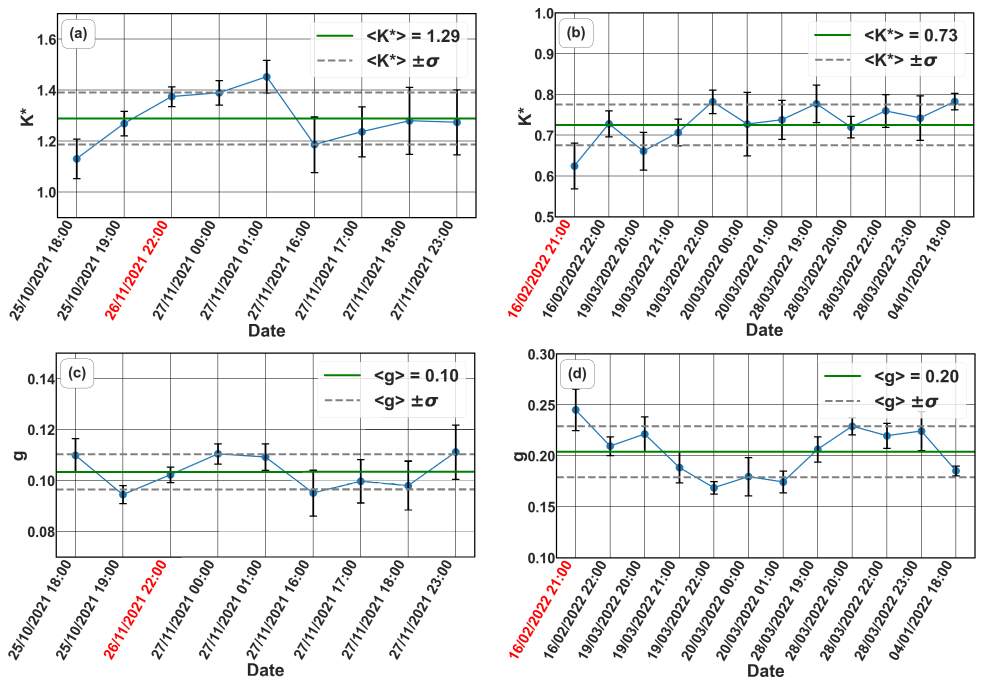
Figure 7 Polarization parameters derived with the two-parameter approach vs. time for the period 1 (a, c) and period 2 (b, d). The error bars represent the derived parameter's variation within the selected comparison ranges $h_{{\mathit{\delta }}_{\mathrm{m}}^{\ast }}$ and $h_{{\mathit{\delta }}_d}$. The average polarization parameter value and its standard deviation in the whole period is given with green and dashed gray lines, respectively. The timestamps of the cases shown in Fig. 6 are highlighted in red.

Table 2 Average polarization parameters for each examined period given with the standard deviation. All values are rounded to two significant figures for the standard deviation.

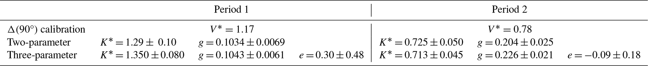
Polarization parameters were calculated for all the chosen profiles during the two specified periods. The resulting polarization parameters are seen in Fig. 7 with error bars representing their variation within the selected comparison ranges $h_{{\mathit{\delta }}_{\mathrm{m}}^{\ast }}$ and $h_{{\mathit{\delta }}_d}$. As depicted in Fig. 7, the parameter time series indicate consistent values with slight fluctuations around their mean. This stability allows us to employ average polarization parameters, as seen in Table 2, for the specified periods. By comparing the average value of g from the table to the values in Fig. 6b, it is evident that the calculated g value for 16 February 2022, 21:00 UTC, was overestimated (g=0.25 compared to g=0.20). This is reflected in the slightly negative values in the lowest ranges of the graph in Fig. 6b. Figure 8 shows the VDR profiles using the average polarization parameters for the two individual cases shown previously in Fig. 6. There is no important effect on the profiles from the application of the average parameters, with low- and high-depolarizing layers being represented well. Any observed variations remain within the uncertainty of the method. The shaded area around the average-parameter corrected profile (brown) shown in Fig. 8 represents the errors associated with the variability of the K^∗ and g parameters during the selected periods and was calculated as described in Appendix D.

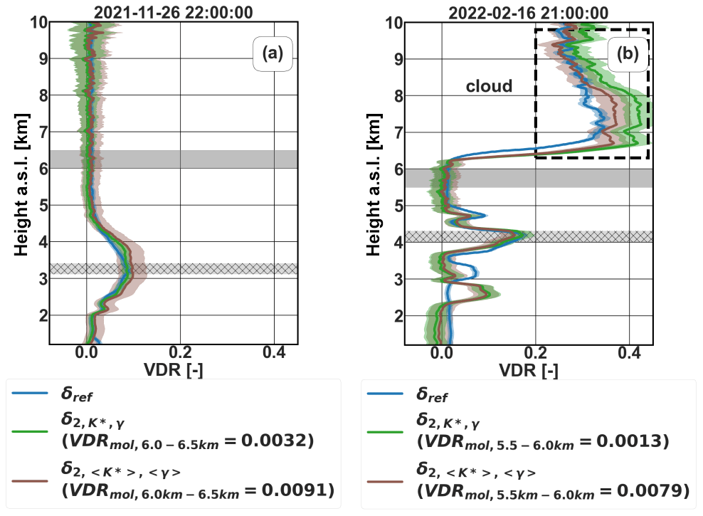
Figure 8 VDR profiles calculated using the two-parameter approach for (a) 26 November 2021, 22:00 UTC, and (b) 16 February 2022, 21:00 UTC, using the profile-specific (blue) and the average (orange) polarization parameters for the two periods. Systematic errors of the reference instrument are shown in blue, and the statistical uncertainty of the corrected profile δ₂ using the average polarization parameters is shown in brown.

4.2 Three-parameter depolarization characterization

In the previous simplified approach, we neglected the e cross-talk constant. In principle, this approximation can introduce errors at the dust and cloud layers (large δ), and we expect the three-parameter approach to fill this gap. The exception to this is for lidar systems, where e is close to 0.

In the three-parameter depolarization characterization, we retrieve all the constants, namely g, e, and K^∗. As there are now three unknowns (Eq. 8), determining the cross-talk constant e requires additional input from the measured aerosol column. In addition to the dust and molecular layers used in the two-parameter approach (${\mathit{\delta }}_{{\mathrm{d}}_{\mathrm{1}}}$ and δ_m), we can use a second dust layer or/and a high-level ice cloud (${\mathit{\delta }}_{{\mathrm{d}}_{\mathrm{2}}}$). Using ice cloud data requires caution due to potential differences in ice crystal orientation measured between systems and due to the distance between the two lidars which may capture different parts of the cloud. Furthermore, the way the lidar is pointed, especially when dealing with oriented ice crystals, and the possibility of multiple scattering effects highlight the importance of carefully interpreting the results when using ice clouds. We apply this here for illustrative purposes in one case only, but we advocate using two aerosol layers whenever possible. The resulting three-parameter equations are

$$\begin{array}{}\text{(15)}& {\displaystyle }{\mathit{\delta }}_{{\mathrm{ref}}_i}={\displaystyle \frac{{\mathit{\delta }}_{{\mathrm{d}}_i}^{\ast }-K^{\ast }g}{K^{\ast }-e{\mathit{\delta }}_{{\mathrm{d}}_i}^{\ast }}}(i=\mathrm{1},\mathrm{2})\text{(16)}& {\displaystyle }{\mathit{\delta }}_{\mathrm{m}}={\displaystyle \frac{{\mathit{\delta }}_{\mathrm{m}}^{\ast }-K^{\ast }g}{K^{\ast }-e{\mathit{\delta }}_{\mathrm{m}}^{\ast }}}.\end{array}$$

This approach introduces an additional constraint to the determination of the parameters. The main reason is that identifying cases with two layers with different depolarization properties measured by both instruments can be rare. As a result of this, reducing the number of selected cases increases the uncertainty of the derived polarization parameters. Moreover, the two independent layers can be advected in a different way; therefore it is not necessarily possible to use the same vertical shift correction for both.

During period 1, it was really difficult to identify profiles with two layers above 3 km, mainly because the dust events remained at lower altitudes. However, with only a few cases, we derived the polarization parameters seen in Table 2.

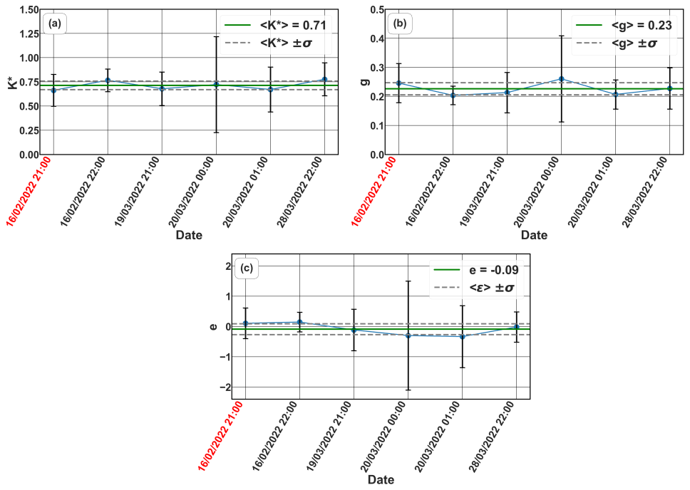
Figure 9 Polarization parameters vs. time for period 2 for the three-parameter approach. The error bars represent the derived parameter's variation within the selected comparison ranges $h_{{\mathit{\delta }}_{\mathrm{m}}^{\ast }}$ and $h_{{\mathit{\delta }}_{\mathrm{d}\mathrm{1},\mathrm{2}}}$.

For period 2, more cases passed the selection criteria mentioned at the beginning of Sect. 4. Figure 9 shows the time dependence of the resulting parameters for period 2 with error bars representing their variance within the comparison ranges $h_{{\mathit{\delta }}_{\mathrm{m}}^{\ast }}$ and $h_{{\mathit{\delta }}_{\mathrm{d}\mathrm{1},\mathrm{2}}}$.

Comparing the polarization parameters from the two approaches (two-parameter vs. three-parameter) in Table 2, g and K^∗ remained almost unchanged, which satisfies our expectations that the effect of g dominates the low-depolarization layers. This is also confirmed by the values of e which are compatible with zero when considering their associated uncertainties. In Fig. 10, the VDR profiles from the two approaches are compared to give a full picture of the vertical deviations. The three-parameter approach tends to yield a smaller VDR across the entire profile range and negative values outside the dust and cloud layers. Additionally, the polarization parameters derived using the three-parameter approach exhibit increased variability compared to the two-parameter approach, as indicated by the error bars in Fig. 10. The shaded error bar region in Fig. 10, representing the uncertainty associated with the three-parameter method (explained in Appendix D), highlights that the discrepancies observed between the two methods, and also the occurrence of negative values, can be explained by the uncertainty on g and e (1 standard deviation). Following these results, we prefer to keep things simple with the two-parameter approach and neglect the effect of e for this instrument.

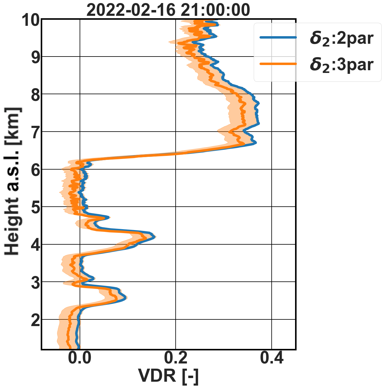
Figure 10 VDR profiles for 16 February 2022, 21:00 UTC, calculated using the two-parameter (blue) and the three-parameter (orange) polarization parameters. The shaded error bar area corresponds to the three-parameter method uncertainty.

4.3 Effective angle of rotation between receiver and emitter

In Freudenthaler et al. (2009), the characterization of depolarization is achieved through knowledge of the channel gain ratio, the beamsplitter transmittances and reflectances, and the angle of rotation ϕ between the polarization of the emitter with respect to the frame of reference of the receiver. With the method presented here, instead, the characterization is achieved through the determination of the parameters K^∗, g, and e. These two representations can be made mathematically equivalent, as shown in Appendix A, and this opens an opportunity to evaluate the angle ϕ from Eq. (A3), using the derived value of g and assuming that the beamsplitter parameters $R_{\mathrm{p}}=\mathrm{1}-T_{\mathrm{p}}$ and $R_{\mathrm{s}}=\mathrm{1}-T_{\mathrm{s}}$ provided by the manufacturer and given in Table 1 are correct. When doing this exercise, we evaluate that $\mathit{\varphi }=(\mathrm{71}\pm \mathrm{1})\mathit{°}$ and $\mathit{\varphi }=(\mathrm{66}\pm \mathrm{1})\mathit{°}$ for periods 1 and 2, respectively. It is to be noted that the derived angle is not the true angle of rotation, given that in our instrument the angle of rotation is minimized and made to be close to 0° by rotation of an HWP in the optical path to maximize the co-polar signal for molecular layers (see Sect. 3.1). We will therefore call ϕ the effective angle of rotation, being a useful parameter to characterize the residual cross-talk in the system. We recall, moreover, that different beamsplitters were used for both periods, and yet the evaluated ϕ of 66–71° does not undergo a huge variation: this may suggest that the issue more likely resides in the emitter (laser depolarization purity), in an incorrect characterization of the PBS, or in additional diattenuation due to other optical components. Note that the calculations in this paper are based on the mathematical model described in Sect. 2, which does not account for the characteristics of the components of the lidar system. The fact that we find such a large effective angle of rotation shows that some unknown error sources in the Cimel lidar are causing the large cross-talk that we observe.

5 Conclusions

We have presented and demonstrated a method for determining the polarization parameters using observations from a reference instrument at a nearby location. Our approach accounts for the cross-talk between the co-polar and cross-polar channels by employing a set of equations that contain three parameters, K^∗, g, and e, using observations from a reference lidar. We examined the ability of this method to characterize VDR observations from a lidar, for which the standard calibration procedures could not fully account for the cross-talk, by utilizing VDR measurements from a reference lidar and a previously calibrated lidar. The aim is to obtain the correct depolarization of dust layers and approach the calculations based on Behrendt and Nakamura (2002) for the molecular layers.

Results are shown for both a simplified version of this method, the two-parameter approach, where the cross-polar interference into the co-polar channel (e) is neglected, and the three-parameter approach, where all parameters are to be retrieved. As a whole, the depolarization characterization approach of this paper corrects the depolarization values of both high- (i.e., dust) and low-depolarizing (i.e., molecular) layers and permits the estimation of the cross-talk parameters. The reliability of the atmospheric depolarization characterization method is supported by observing reduced discrepancies in the VDR when compared to expected VDR values at molecular layers. The relative difference in VDR to the reference observations at dust layers is less than 1 % after the application of the two-parameter approach.

The application of the three-parameter approach was more challenging, mainly due to there being few cases which satisfy the criterion of having two independent aerosol layers above 3 km in one profile. Based on these cases the recalculated parameters K^∗ and g did not change more than 5 %. We found from the results of the three-parameter approach that e was compatible with 0 considering its uncertainty and could therefore be neglected, thus justifying the two-parameter approach.

The calculated polarization parameters from different cases (9 and 12 timestamps for the periods 1 and 2, respectively) vary little over the examined periods, allowing us to apply average parameters calculated for the specific system for calculating the VDR over longer periods, as was shown in this study. The application of the average instead of the profile-specific polarization parameters leads to negligible differences at the high- and low-depolarized layers, which is acceptable as it remains within the uncertainty of the method. Nevertheless, the system's degradation could affect the polarization parameters; therefore, it is suggested that these are re-evaluated on a seasonal basis and at every system upgrade. The applied polarization parameters are found to reduce significantly the VDR discrepancies between the tested and the reference lidar in cases where distinct and similar dust layers are observed, thus justifying their retrospective application to be able to use existing valuable data acquired during campaigns.

The EARLINET campaign 2009 (EARLI09) suggests a detailed methodology on the intercomparison approach, requiring all systems to be placed side by side for several days before being deployed at their measuring locations, in order to be able to combine observations from different instruments and techniques (Wandinger et al., 2016). We need to emphasize that this was not possible in our case, as we are attempting a retrospective characterization of Cyprus 2021 Fall Campaign observations. However, these guidelines should be followed whenever possible, and, for the future, we plan an upgrade of the system to have a reliable calibration upfront.

This depolarization characterization method, demonstrated here for the first time, provides a good alternative for systems for which the user does not know the values of g and e a priori; therefore, it can be applied where traditional calibration procedure fails to correct the cross-talk in the depolarization channels. According to Bravo-Aranda et al. (2013), lidar systems which are not well characterized and well aligned can lead to large systematic errors in the depolarization values. Reducing the errors related to the depolarization observations will therefore reduce the total uncertainty of aerosol typing studies (e.g., Mamouri and Ansmann, 2014) or mass concentration retrievals (e.g., Mamali et al., 2018), for which the particle linear depolarization ratio is a key parameter.

It is noteworthy to highlight that, in the work of Freudenthaler (2016), a comprehensive theoretical framework for depolarization calibration was introduced, significantly expanding the scope of influencing quantities and parameters. A different approach for atmospheric calibration would be to apply an intercomparison that takes into account these parameters and includes a more comprehensive error calculation.

Using the presented method, valuable data obtained during the Fall Campaign 2021 in Cyprus (Kezoudi et al., 2022) can be corrected and used for further research on aerosol characteristics and stratification.

Appendix A: How the present treatment of depolarization relates to Freudenthaler et al. (2009)

Freudenthaler et al. (2009) treated lidar depolarization extensively and introduced the Δ(90°) method for calibration, which is nowadays of widespread use and a de facto standard. We relate here their equations to the ones developed in Sect. 2. Whereas in Sect. 2 we do not make any assumptions on the technology employed, the treatment in that paper assumes that the two polarization components are separated in the receiver by means of a polarizing beamsplitter cube (PBS) of known characteristics and that the emitted beam polarization plane may be rotated with respect to the PBS reference system. We rewrite here their Eq. (9) for convenience:

$$\begin{array}{}\text{(A1)}& {\mathit{\delta }}_F^{\ast }=V^{\ast }{\displaystyle \frac{R_{\mathrm{p}}\left(\mathrm{1}+\mathit{\delta }{\tan }^{\mathrm{2}}\mathit{\varphi }\right)+R_{\mathrm{s}}\left({\tan }^{\mathrm{2}}\mathit{\varphi }+\mathit{\delta }\right)}{T_{\mathrm{p}}\left(\mathrm{1}+\mathit{\delta }{\tan }^{\mathrm{2}}\mathit{\varphi }\right)+T_{\mathrm{s}}\left({\tan }^{\mathrm{2}}\mathit{\varphi }+\mathit{\delta }\right)}},\end{array}$$

where ${\mathit{\delta }}_F^{\ast }$ is the ratio of the two lidar signals, V^∗ is the channel gain ratio, and ϕ is the angle between the plane of polarization of the laser and the incidence plane of the PBS. R_p, R_s, T_p, and T_s indicate the reflectivities and transmittances of the PBS for linearly polarized light parallel (p) and perpendicular (s) to the incidence plane, with $R_{\mathrm{p}}\simeq \mathrm{1}-T_{\mathrm{p}}$ and $T_{\mathrm{s}}\simeq \mathrm{1}-R_{\mathrm{s}}$. The reason why we use the symbols ${\mathit{\delta }}_F^{\ast }$ instead of δ^∗ and V^∗ instead of K^∗ will be apparent in the following.

This equation has to be compared to our Eq. (7). The lidar PBS can basically be installed in two logical configurations: with ϕ close to 0° or with ϕ close to 90°. In the first case, ${\mathit{\delta }}_F^{\ast }={\mathit{\delta }}^{\ast }$, by comparing Eqs. (A1) and (7), one finds that

$$\begin{array}{}\text{(A2)}& K^{\ast }=V^{\ast }{\displaystyle \frac{R_{\mathrm{p}}{\tan }^{\mathrm{2}}\mathit{\varphi }+R_{\mathrm{s}}}{T_{\mathrm{p}}+T_{\mathrm{s}}{\tan }^{\mathrm{2}}\mathit{\varphi }}}.\end{array}$$

Note that in cases where $R_{\mathrm{s}},T_{\mathrm{p}}\ll \mathrm{1}$ (like in the case of CE376) or $R_{\mathrm{p}},T_{\mathrm{s}}\ll \mathrm{1}$ (like in the cases of other lidars in the literature), Eq. (A2) can be reduced to $K^{\ast }\simeq V^{\ast }$.

$$\begin{array}{}\text{(A3)}& {\displaystyle }g={\displaystyle \frac{R_{\mathrm{p}}+R_{\mathrm{s}}{\tan }^{\mathrm{2}}\mathit{\varphi }}{R_{\mathrm{p}}{\tan }^{\mathrm{2}}\mathit{\varphi }+R_{\mathrm{s}}}}\text{(A4)}& {\displaystyle }e={\displaystyle \frac{T_{\mathrm{p}}{\tan }^{\mathrm{2}}\mathit{\varphi }+T_{\mathrm{s}}}{T_{\mathrm{p}}+T_{\mathrm{s}}{\tan }^{\mathrm{2}}\mathit{\varphi }}}\end{array}$$

In cases where the system has ϕ=90° and then ${\mathit{\delta }}_F^{\ast }=\mathrm{1}/{\mathit{\delta }}^{\ast }$, equations equivalent to the above can be derived with a simple derivation (omitted for brevity), and $V^{\ast }\simeq \mathrm{1}/K^{\ast }$.

Appendix B: How the present treatment of depolarization relates to Freudenthaler et al. (2016)

Freudenthaler (2016) provided general formulations for calculating the linear volume depolarization ratio for different lidar setups considering various error sources stemming from different components from the laser to the detector. The errors can stem from rotational misalignments and cross-talks. The general formula for volume depolarization ratio is given in Eq. (62) of Freudenthaler (2016) and is

$$\begin{array}{}\text{(B1)}& \mathit{\delta }={\displaystyle \frac{{\mathit{\delta }}^{\ast }(G_T+H_T)-(G_R+H_R)}{(G_R-H_R)-{\mathit{\delta }}^{\ast }(G_T-H_T)}},\end{array}$$

where G_T, G_R, H_T, and H_R describe the polarization cross-talk terms of the lidar setup in the reflected (R) and transmitted paths (T).

By comparing this equation to Eq. (10) of this paper, one finds that

$$\begin{array}{}\text{(B2)}& {\displaystyle }{K}^{\ast }={\displaystyle \frac{G_R-H_R}{G_T+H_T}}\text{(B3)}& {\displaystyle }g={\displaystyle \frac{G_R+H_R}{G_R-H_R}}\text{(B4)}& {\displaystyle }e={\displaystyle \frac{G_T-H_T}{G_T+H_T}}.\end{array}$$

Therefore, the calculation of K^∗, g, and e can lead to G_T, G_R, H_T, and H_R and vice versa. This means that g and e parameters obtained through lidar comparison with a reference instrument can be linked to the cross-talk terms computed from the instrument's internal components (if known).

Appendix C: Vertical shift correction due to spatial separation

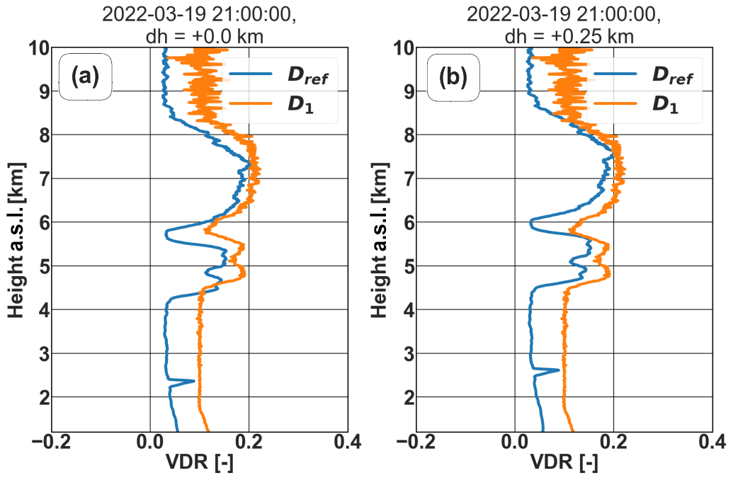
A vertical shift appears in the comparison of the profiles of the two instruments mainly due to sloping atmospheric layers between Limassol and Nicosia. This shift can be observed when comparing the most important common dust or cloud layers. A vertical correction is applied on one of the lidar profiles in order to bring the interesting layers to the same altitudes as the second lidar. An example of this correction is seen in Fig. C1, where we consider a vertical correction of dh=0.25 km for the selected timestamp.

Figure C1 VDR profiles without (a) and with (b) vertical correction.

Appendix D: Uncertainty analysis

The corrected values of δ are subject to the propagation of uncertainty. The uncertainty of the presented two-parameter approach can be calculated according to BIPM et al. (2009) as follows:

$$\begin{array}{}\text{(D1)}& \begin{array}{rl}{\left(\mathrm{\Delta }\mathit{\delta }\right)}^{\mathrm{2}}=& f\left(\mathrm{\Delta }{K}^{{\ast }^{\mathrm{2}}},\mathrm{\Delta }{g}^{\mathrm{2}},\mathrm{\Delta }{\mathit{\delta }}^{{\ast }^{\mathrm{2}}}\right)\\ =& \left[{\left({\displaystyle \frac{\mathrm{\Delta }{\mathit{\delta }}^{\ast }}{{\mathit{\delta }}^{\ast }}}\right)}^{\mathrm{2}}+{\left({\displaystyle \frac{\mathrm{\Delta }{K}^{\ast }}{K^{\ast }}}\right)}^{\mathrm{2}}\right]{\left({\displaystyle \frac{{\mathit{\delta }}^{\ast }}{K^{\ast }}}\right)}^{\mathrm{2}}+{\left(\mathrm{\Delta }g\right)}^{\mathrm{2}}\\ =& \left[{\left({\displaystyle \frac{\mathrm{\Delta }{P}^{\perp }}{P^{\perp }}}\right)}^{\mathrm{2}}+{\left({\displaystyle \frac{\mathrm{\Delta }{P}^{\parallel }}{P^{\parallel }}}\right)}^{\mathrm{2}}+{\left({\displaystyle \frac{\mathrm{\Delta }{K}^{\ast }}{K^{\ast }}}\right)}^{\mathrm{2}}\right]\\ & {\left({\displaystyle \frac{P^{\perp }}{P^{\parallel }{K}^{\ast }}}\right)}^{\mathrm{2}}+{\left(\mathrm{\Delta }g\right)}^{\mathrm{2}}.\end{array}\end{array}$$

In the above equation, ΔK^∗ and Δg are the statistical uncertainties of the parameters within the chosen interval (e.g., the standard deviation presented in Table 2). The measurement uncertainties ΔP^⊥ and ΔP^∥ for each polarization channel consist of the uncertainty of the raw counts signal (P₀) and the background correction (B). As the signal is received by a photon-counting detector, the distribution of the counts follows Poisson statistics; therefore the standard deviation is given by the square root of the number of counts in the measured interval (N).

$$\begin{array}{}\text{(D2)}& \mathrm{\Delta }{P}^{\perp ,\parallel }=\sqrt{\left(\mathrm{\Delta }{P_{\mathrm{0}}}^{\mathrm{2}}\right)+\left(\mathrm{\Delta }{B}^{\mathrm{2}}\right)}=\sqrt{N+{\displaystyle \frac{\mathit{\sigma }(B{)}^{\mathrm{2}}}{n}}},\end{array}$$

where σ(B) is the standard deviation of the background correction calculated over n=67 ranges, which corresponds to 1 km.

These calculations are used for deriving the error bars of the two-parameter correction profiles seen in Figs. 6 and 8.

The uncertainty of δ in the three-parameter approach is also dependent on Δe; therefore $(\mathrm{\Delta }\mathit{\delta }{)}^{\mathrm{2}}=f(\mathrm{\Delta }{K^{\ast }}^{\mathrm{2}},\mathrm{\Delta }{g}^{\mathrm{2}},\mathrm{\Delta }{e}^{\mathrm{2}},\mathrm{\Delta }{{\mathit{\delta }}^{\ast }}^{\mathrm{2}})$. We omit the equations here for brevity.

Appendix E: CE376 optomechanical setup

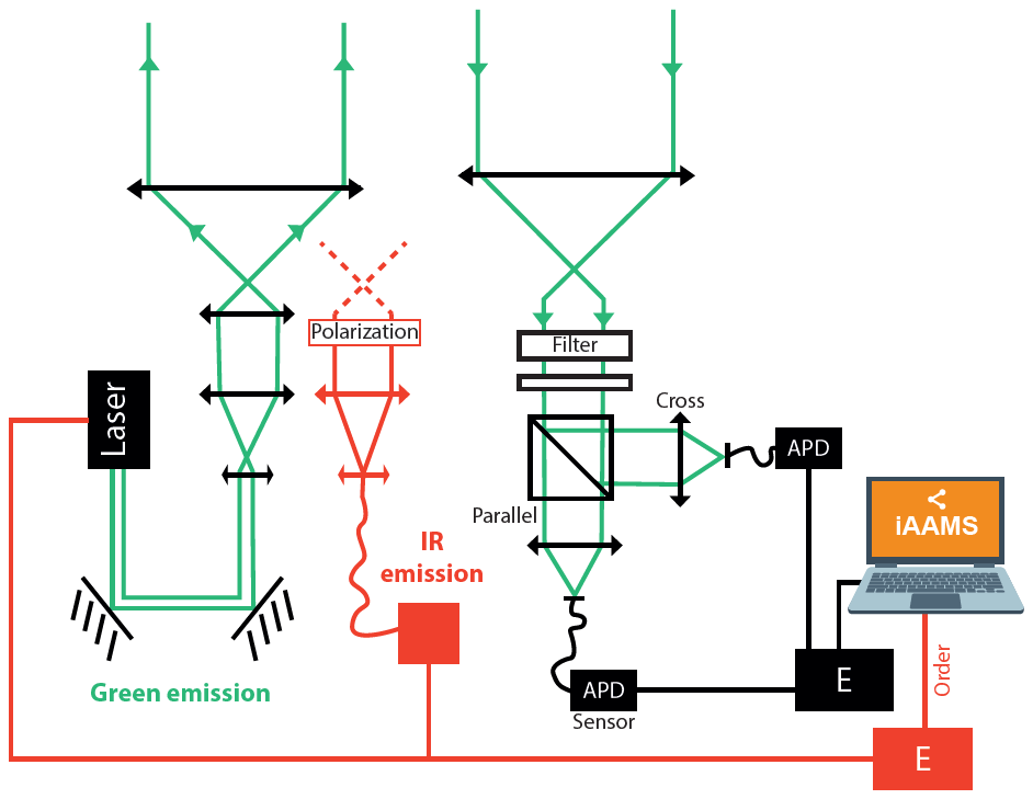
The CE376 consists of two lasers: a double-frequency Nd:YAG emitting at 532 nm and a pulsed laser diode for near-infrared (NIR). The backscattered radiation is collected by a Galilean telescope with a diameter of 100 mm both in emission and reception. In the detection branch after the telescopes, the following can be found: a narrow filter for reducing the background light, a half-wave plate to rotate the plane of polarization, and a beamsplitter cube to separate the parallel and cross-polarized signals received in the 532 nm channel. The signals are recorded by avalanche photodiodes (APDs by SPCM-AQRH modules from Excelitas) at the three reception channels. The APDs are capable of detecting single-photon events.

Figure E1 Schematic of the CE376 optomechanical setup.