Application of fuzzy c-means clustering for analysis of chemical ionization mass spectra: insights into the gas phase chemistry of NO₃-initiated oxidation of isoprene

Oxidation of volatile organic compounds (VOCs) can lead to the formation of secondary organic aerosol (SOA), a significant component of atmospheric fine particles, which can affect air quality, human health, and climate change. However, the current understanding of the formation mechanism of SOA is still incomplete, which is not only due to the complexity of the chemistry but also relates to analytical challenges in SOA precursor detection and quantification. Recent instrumental advances, especially the development of high-resolution time-of-flight chemical ionization mass spectrometry (CIMS), greatly improved both the detection and quantification of low- and extremely low-volatility organic molecules (LVOCs/ELVOCs), which largely facilitated the investigation of SOA formation pathways. However, analyzing and interpreting complex mass spectrometric data remain a challenging task. This necessitates the use of dimension reduction techniques to simplify mass spectrometric data with the purpose of extracting chemical and kinetic information of the investigated system. Here we present an approach to apply fuzzy c-means clustering (FCM) to analyze CIMS data from a chamber experiment, aiming to investigate the gas phase chemistry of the nitrate-radical-initiated oxidation of isoprene.

The performance of FCM was evaluated and validated. By applying FCM to measurements, various oxidation products were classified into different groups, based on their chemical and kinetic properties, and the common patterns of their time series were identified, which provided insight into the chemistry of the investigated system. The chemical properties of the clusters are described by elemental ratios and the average carbon oxidation state, and the kinetic behaviors are parameterized with a generation number and effective rate coefficient (describing the average reactivity of a species) using the gamma kinetic parameterization model. In addition, the fuzziness of FCM algorithm provides a possibility for the separation of isomers or different chemical processes that species are involved in, which could be useful for mechanism development. Overall, FCM is a technique that can be applied well to simplify complex mass spectrometric data, and the chemical and kinetic properties derived from clustering can be utilized to understand the reaction system of interest.

1 Introduction

Volatile organic compounds (VOCs) in the atmosphere are oxidized by reactions with hydroxyl radicals (OH), ozone (O₃), nitrate radicals (NO₃), or Cl atoms, leading to the formation of condensable vapors such as low- and extremely low-volatility organic compounds (LVOCs/ELVOCs) that subsequently condense onto existing particles or even form new particles and thereby form secondary organic aerosol (SOA) (Donahue et al., 2012; Hallquist et al., 2009; Ziemann and Atkinson, 2012). SOA comprises a major fraction of the atmospheric submicron particulate matter and can have an adverse impact on air quality, human health, and climate (Hallquist et al., 2009; Jimenez et al., 2009; Pöschl, 2005; Spracklen et al., 2011; Zhang et al., 2007). Despite extensive studies on characterization of the products and mechanisms involved in VOC oxidation and SOA formation, how VOCs contribute to SOA formation is not yet fully understood. This is not only hampered by the complexity of the chemistry itself but also by the remaining analytical challenges in the detection of organic precursors with low volatility (Bianchi et al., 2019; Shrivastava et al., 2017).

Recent instrumental developments, especially the availability of high-resolution time-of-flight chemical ionization mass spectrometry (CIMS) in atmospheric research, made the direct detection of low-volatility vapors possible (Ehn et al., 2012, 2014; Jokinen et al., 2015). Benefitting from this, it has been discovered that the highly oxygenated organic molecules (HOMs), which are formed through a rapid gas phase process called autooxidation and generally have very low volatilities, significantly contribute to SOA and even new particle formation (Crounse et al., 2013; Ehn et al., 2012, 2014; Kirkby et al., 2016; Praske et al., 2018).

While advanced mass spectrometers greatly enhance our capability to detect and quantify HOMs and facilitate the investigation of the HOM formation mechanism, the highly complex mass spectrometric data, which consist of hundreds to thousands of variables (i.e., detected ions) over thousands of points in time, make the data processing and interpretation challenging. In addition, the mass spectrometers are unable to detect structures of molecules, despite modern instruments with high resolution (e.g., over 10 000 $m/\mathrm{\Delta }m$​​​​​​​) (Breitenlechner et al., 2017; Krechmer et al., 2018), which significantly hinders the understanding of the chemical processes involved. Furthermore, it is difficult to refine and extract kinetic and mechanistic information directly from the mass spectrometric data.

To reduce the complexity of data analysis, dimension reduction techniques are necessary, which compress various variables in a dataset into a few to a dozen of factors/clusters based on the underlying correlation/similarity of different variables, e.g., in terms of their sources or physicochemical properties, while retaining the major chemical and kinetic information of investigated systems and thus making the data analysis easier and more effective (Äijälä et al., 2017; Buchholz et al., 2020; Koss et al., 2020; Yan et al., 2016; Zhang et al., 2019).

Factorization is one of the major dimension reduction techniques within which positive matrix factorization (PMF) (Paatero, 1997; Paatero and Tapper, 1994) is the most commonly used approach in atmospheric science, especially for ambient measurements of particulate matter by aerosol mass spectrometry (Canonaco et al., 2013; Lanz et al., 2007, 2008; Zhang et al., 2005, 2011), as well as for VOC measurements in both field and laboratory studies (Brown et al., 2007; Lanz et al., 2009; Li et al., 2021; Rosati et al., 2019; Vlasenko et al., 2009; Yuan et al., 2012). Principal component analysis (PCA) (Wold et al., 1987) is also a frequently used multivariate factor analysis technique for the deconvolution and interpretation of gas and particle phase composition data (Sofowote et al., 2008; Wyche et al., 2015; Zhang et al., 2005). Additionally, non-negative matrix factorization (NMF), which is very similar to the PMF approach, has been widely used in interdisciplinary fields (Devarajan, 2008; Fu et al., 2019; Lee and Seung, 1999), as well as in atmospheric science (Chen et al., 2013; Karl et al., 2018; Malley et al., 2014; Song et al., 2021). Despite the similarities in mathematical formulation and constraints to PMF, the NMF algorithm does not need an error matrix as input. This eliminates the potential impact of error estimation on outcomes and makes it more user-friendly.

In addition to factorization methods, an increasing number of recent studies have applied clustering techniques to mass spectra data (Äijälä et al., 2017; Koss et al., 2020; Li et al., 2020; Priestley et al., 2021). For example, Äijälä et al. (2017) combined a clustering algorithm, k-means $++$, with PMF to classify and characterize the organic component of air pollution plumes detected by aerosol mass spectrometry (AMS). Li et al. (2020) developed a clustering algorithm named noise-sorted scanning clustering, based on the traditional density-based special clustering of applications combined with a noise algorithm and thereafter applied this method to distinguish different types of thermal properties of various biogenic SOA. Koss et al. (2020) compared the performance of hierarchical clustering analysis (HCA) with PMF and gamma kinetics parameterization for the analysis of complex mass spectrometric data. Their results demonstrate the feasibility of using HCA to identify major types of ions and patterns of time behavior and to draw out bulk chemical properties of the system that can be useful for modeling. In addition, in a recent work by Priestley et al. (2021), HCA was applied to infer the CHON functionality of products formed from benzene oxidation.

In this work, we choose the fuzzy c-means clustering algorithm (FCM) as the major technique to analyze CIMS data collected from a chamber experiment, aiming to investigate the gas phase chemistry of the isoprene–NO₃ oxidation system. Isoprene is the most abundant biogenic volatile organic compound (BVOC) on Earth and is highly reactive in the atmosphere, which is an important precursor of O₃ and SOA, and thus imposes detrimental effects on climate and health (Carlton et al., 2009; Surratt et al., 2019). The reaction of isoprene with NO₃ is an important source of SOA, but its gas phase reaction mechanism, especially the multi-generation chemistry and the contribution of the corresponding oxidation products to SOA formation remain ambiguous at present (Carlton et al., 2009; Fry et al., 2018; Ng et al., 2008; Rollins et al., 2009; Wu et al., 2021). Fuzzy c-means clustering is the most widely used fuzzy clustering algorithm and is adopted in this study considering the following three aspects. First, FCM allows variables to be affiliated with multiple clusters, similar to factorization methods like PMF, NMF, and PCA. Conversely, hard clustering methods, such as the most popular k-means clustering, assign each variable exclusively into one cluster. In atmospheric chemistry, one compound can originate from several different sources, or a detected species may consist of isomers produced from different chemical processes. Therefore, from this perspective, assigning a variable to multiple clusters with a quantified membership degree is more rational than assigning variables to mutually exclusive clusters. Second, FCM is more user-friendly, since only the data matrix is needed as input, whereas additional information is required for factor analysis methods, such as the error matrix needed in PMF. Furthermore, receptor models like PMF assume that the factor profiles remain constant over time and that the chemical species do not react with each other during the sampling period (Chen et al., 2011; Reff et al., 2007; Xie et al., 2022), which is not the case for chamber measurements.

Using FCM, variables with similar time behaviors will be grouped into the same cluster, and the centroid of the cluster (cluster center) can be used as a surrogate for these variables. Therefore, the numerous species detected in a chemical system can be compressed to a much smaller number of clusters, each of which represents a typical chemical process/source with unique time behavior. By analyzing these cluster centers instead of the whole dataset, one can obtain the chemical and kinetic properties of the investigated system in a much easier way. The significant reduction in the complexity of data analysis and the chemical and kinetic information derived from this method can help with a better understanding of the chemical system of interest (Koss et al., 2020). In addition, to evaluate its performance, we applied FCM to a synthetic dataset derived from a box model with an explicit mechanism. By exemplifying the functionality of such a clustering method in analyzing CIMS data, we propose that FCM is a useful method that offers a new approach to analyzing mass spectrometric data and to deriving useful information on chemical and kinetic properties of products that can help decipher the underlying reaction mechanism.

2 Methods

2.1 Data collection and processing

The experimental data used in this work were collected in the atmospheric simulation chamber SAPHIR (Simulation of Atmospheric PHotochemistry In a large Reaction Chamber) at the Forschungszentrum Jülich, Germany, during the ISOPNO₃ campaign in 2018. The SAPHIR chamber is a double-walled Teflon (PEP) cylinder, with an approximate volume of 270 m³ (5 m in diameter; 20 m in length). It is fixed by an aluminum frame with movable shutters that can be opened or closed to simulate daytime or nighttime chemistry. Trace gases in the chamber can be well mixed within 2 min with the help of two continuously operated fans. During an experiment, the chamber is filled with synthetic air and kept slightly overpressured (∼ 35 Pa) to prevent permeation of outside air into the chamber. Due to small leakages and instrument sampling consumption, there is a replenishing flow into the chamber, which leads to a dilution rate of 4 % h⁻¹–7 % h⁻¹. More details about the chamber setup and its performance can be found elsewhere (Rohrer et al., 2005).

The experiment selected here was conducted to characterize the gas phase chemistry of the NO₃-initiated oxidation of isoprene. O₃ and NO₂ were added in sequence to produce NO₃, followed by the addition of ∼ 10 ppbv of isoprene to initiate the reaction. The injections were repeated four times (only NO₂ and O₃ were added in the last injection) to build up products and to facilitate later-generation oxidation. The mixing ratios of O₃ and NO₂ in the chamber were approximately 100 and 25 ppbv, respectively, after the first injection, as shown in Fig. S1 in the Supplement. A detailed description of the experimental procedure can be found elsewhere (Wu et al., 2021).

During the campaign, a comprehensive set of instruments was deployed to measure radicals and closed-shell products in both gas and particle phase, as described by Wu et al. (2021). In this work, however, we focus on the measurements acquired by a high-resolution time-of-flight chemical ionization mass spectrometer (Aerodyne Research Inc.), using Br⁻ as reagent ion, which detected the HO₂ radical and the gas phase products generated by the reaction of isoprene and NO₃. The mass spectrometer was operated in V mode with a mass resolution of 3000–4000 ($m/\mathrm{\Delta }m$​​​​​​​). A customized inlet was designed to connect the CIMS directly to the chamber to reduce losses of the HO₂ radical and HOM in the sampling line (Albrecht et al., 2019). More information about settings and performance of the instrument can be found in our previous study (Wu et al., 2021).

The raw mass spectrometric data were processed using the Tofware toolkit (v. 2.5.11, Tofwerk AG and Aerodyne Research Inc.) in Igor Pro (v.7.0.8, WaveMetrics), following the routines described by Stark et al. (2015). High-resolution peak fitting was conducted in the mass range of $m/z$ 60–600 to identify the chemical composition of detected ions. For the high-resolution peak assignment, we fitted the observed peaks using predefined instrument functions (including peak shape, peak width as a function of $m/z$, and baseline). If necessary, contributions of more than one component were considered for the fit in order to reduce the residuals of the fitting. Once the peak numbers and peak positions were fixed, the chemical formula (consisting of C, H, O, and N atoms) of each peak was assigned manually by selecting from a formula list generated by the software. During the peak fitting, isotopes were constrained, and only plausible formulas with relative $m/z$ deviations smaller than 10 ppm were considered. In addition, only molecule formulas with a time behavior commensurable with expectations for the specific chemical system were assigned (Pullinen et al., 2020). For example, it is illogical if large amounts of organonitrates are observed under low-NO_x conditions.

Overall, around 160 ions were identified by the Br⁻ CIMS. The background signal of each ion was determined from measurements prior to precursor injection and was subtracted from the signal measured in the chamber. These ions consist of species related to real isoprene oxidation products, as well as other signals related to the ion source, internal standard, and interferences from chamber and tubing. The product ions are those produced by isoprene oxidation, and they should have visible changes (either increase or decrease) when the chemistry is initiated or modified. A simple way to sort the product ions from other chemically irrelevant signals is to examine the time evolution of each ion. By comparing the signals before and after each injection, we can easily distinguish the product ions from others. Among all the identified ions, a total of 91 ions were recognized as product signals. Since we intend to investigate the underlying chemical relationships of different products through their time behavior and not the absolute concentration, normalized (to the sum of total ion counts) signals were used for further analysis. Calibration procedures are described in more detail elsewhere (Wu et al., 2021).

In addition to abovementioned chamber data, we use a synthetic dataset from a box model with the default gas phase reaction schemes of isoprene–NO₃ taken from the Master Chemical Mechanism (MCM) version 3.3.1 (Jenkin et al., 2015). For the modeling, temperature, relative humidity, and dilution rate were constrained using measured data. The initial concentrations of O₃, NO₂, and isoprene were added into the model according to the experiment schedule. Overall, the modeled concentrations of O₃, NO₂, NO₃, and isoprene match the measurements well (Fig. S2). The synthetic data were used to learn about the principal behaviors of the time series (of products) in a complex chemical system with an established complex mechanism. A detailed description of the isoprene–NO₃ chemistry and evaluation of the model performance are outside the scope of this work. An updated mechanism for isoprene oxidation by NO₃ has been published recently by Carlsson et al. (2023).

2.2 Fuzzy c-means clustering (FCM)

Clustering is one of the major dimension reduction techniques besides factorization, which groups a set of objects into a certain number of clusters according to their (dis)similarities, which are generally measured by a distance metric, such that objects within each cluster are much closer to each other than to those pertaining to other clusters (Hastie et al., 2009). The notion of a fuzzy set, first proposed by Zadeh (1965), gives an idea how to deal with data with indistinct boundaries of clusters. Based on this concept, Bezdek et al. (1984) developed the fuzzy c-means clustering algorithm. In contrast to the hard clustering counterparts like k-means and k-medoids clustering, FCM allows each object to belong to multiple clusters with the membership degree measured by a value varying from 0 to 1 (Bezdek et al., 1984). Consequently, fuzzy clustering can deal with non-discrete data better and thus is adopted here to analyze CIMS data obtained from isoprene–NO₃ oxidation.

Fuzzy c-means clustering is one of the best-known fuzzy clustering algorithms by virtue of its simplicity, quick convergence, and wide applicability (Ghosh and Dubey, 2013; Ren et al., 2016; Yang, 1993). It is a distance-based cluster assignment method, and its working principle is very similar to that of the k-means algorithm. FCM is conducted through an iterative process which attempts to group all objects within a dataset into a predefined number of clusters (c) with a degree of membership and simultaneously minimize the sum of squared distance between the member objects and the cluster centroids, as defined in Eq. (1):

$$\begin{array}{}\text{(1)}& J_m\left(\mathbf{V},\mathbf{U}\right)=\sum _{i=\mathrm{1}}^c\sum _{j=\mathrm{1}}^n{u}_{ij}^m{d}_{ij}^{\mathrm{2}},\end{array}$$

where x_j is the object j in the dataset; u_ij is the membership degree of x_j to the ith cluster, which is enforced to satisfy $u_{ij}\in [\mathrm{0},\mathrm{1}]$ and $\sum _{i=\mathrm{1}}^c{u}_{ij}=\mathrm{1}$; d_ij denotes the distance between object x_j and the ith cluster center v_i; and m is the fuzzifier ($m\in [\mathrm{1},\mathrm{\infty })$) that controls the fuzziness level of the clustering.

Starting with an initial fuzzy partition matrix (U⁰), either provided or randomly produced, the cluster centers (V) are calculated by

$$\begin{array}{}\text{(2)}& v_i={\displaystyle \frac{\sum _{j=\mathrm{1}}^n{u}_{ij}^m\cdot x_j}{\sum _{j=\mathrm{1}}^n{u}_{ij}^m}}\end{array}$$

for all i ($\mathrm{1}\le i\le c$), and afterwards, the membership degrees of each object are updated by

$$\begin{array}{}\text{(3)}& u_{ij}={\left\{{\sum }_{k=\mathrm{1}}^c{\left({\displaystyle \frac{d_{ij}}{d_{kj}}}\right)}^{\frac{\mathrm{2}}{(m-\mathrm{1})}}\right\}}^{-\mathrm{1}}.\end{array}$$

The algorithm proceeds by repeating the above process, and every iteration generates two new sets of V and U. The iteration ends when the algorithm converges (no significant change with further iteration, namely $\Vert U^{(t+\mathrm{1})}-U^{\left(t\right)}\Vert ={max}_{i,j}\mathit{\left\{}\right|u_{ij}^{(t+\mathrm{1})}-u_{ij}^t\left|\mathit{\right\}}<\mathit{\epsilon }$) or the predefined maximum number of iterations is reached. In this study, the FCM algorithm was implemented using the open-source scikit-fuzzy (v 0.4.2) package (https://pypi.org/project/scikit-fuzzy/, last access: 30 December, 2023) in Python.

2.3 Clustering parameters

As noted in Sect. 2.2, several parameters need to be specified ahead of executing FCM, including the number of clusters, the distance metric to measure the (dis)similarity of objects, the value of the fuzzifier, the initial fuzzy partition matrix, the maximum number of iterations, and the stopping criterion. All these parameters can affect the partition outcomes, and among them, the most important ones are the cluster number, the distance metric, and the fuzziness index. A brief introduction to these parameters and the methods to determine their optimal values are given in the following sections.

2.3.1 Number of clusters (c)

Figuring out the optimal number of clusters (c) is one of the challenges in cluster analysis. The optimal number of clusters is related to the structure of the investigated dataset, and it has a critical impact on clustering outcomes. To our knowledge, none of the existing methods are feasible for the determination of the optimal cluster number in all possible cases and applications.

The frequently used method to address this problem is to set the search range of c, conducting clustering to generate solutions according to the predefined number of clusters, and then choosing one or several clustering validity indices (CVIs) to evaluate the outcomes. By comparing the values of the CVI(s) of alternative clustering solutions obtained with different numbers of clusters, the appropriate c could be determined accordingly.

In this case, a validity index is used as a fitness function to evaluate the quality of the clustering results in terms of the intra-cluster compactness and inter-cluster separation. In addition, CVIs play an extremely important role in automatically determining the appropriate number of clusters. Plenty of CVIs have been proposed in the past. Generally, these CVIs can be divided into three categories. The first type of CVI only considers the property of the membership degree in the calculation, such as the partition coefficient (Bezdek and Pal, 1998) and partition entropy (Simovici and Jaroszewicz, 2002), which are also the earliest validity indices for fuzzy clustering. The main disadvantage of such CVIs is that they lack a direct connection to the geometry structure of the data. Considering this, another type of CVI, such as the Fukuyama–Sugeno index (Fukuyama and Sugeno, 1989), Xie–Beni index (Xie and Beni, 1991), Kwon index (Kwon, 1998) and Bouguessa–Wang–Sun index (Bouguessa et al., 2006), was proposed, which takes both membership degree and the geometry structure of dataset into consideration. Given their advantages over those in the first category, we only chose CVIs belonging to the second category in this study. Different from the first two types of CVIs, the third type of CVI makes use of the concept of hypervolume and density for evaluation. The fuzzy hypervolume and the average partition density (Gath and Geva, 1989) are the most popular two indices in this category. In this study, the second type of CVI was chosen for the analysis, considering its applicability to our dataset.

Although there are various types of CVIs, no CVI can always outperform others due to their own limitations and the complexity of different datasets (Kryszczuk and Hurley, 2010; Wang et al., 2021). Generally, each CVI only attaches importance to a specific aspect or limited aspects of a clustering solution, while other aspects can be inadequately represented or even overlooked (Kryszczuk and Hurley, 2010). In order to overcome or at least diminish the impact from this result, we adopt multiple CVIs for the evaluation in this study. Among all the alternatives, the following six CVIs were chosen, including the sum of within-cluster variance (V_SWCV; elbow method), Fukuyama–Sugeno index (V_FS), Xie–Beni index (V_XB), Kwon index (V_Kwon), Bouguessa–Wang–Sun index (V_BWS), and fuzzy silhouette (FS; Campello and Hruschka, 2006). They are the most frequently used CVIs in the literature and are reported to perform well (Bouguessa and Wang, 2004; Campello and Hruschka, 2006; Rawashdeh and Ralescu, 2012; Zhou et al., 2014). More information about these CVIs can be found in Sect. S1 in the Supplement.

With respect to the search range of c, a rule of thumb suggests that the maximum c should not exceed $\sqrt{n}$ (n here is the number of elements in a dataset) (Ren et al., 2016; Yu and Cheng, 2002). Therefore, the search range of c could be set to $[\mathrm{2},\sqrt{n}+\mathrm{1}]$ in general. To obtain a concrete result, for each c in this range, the FCM algorithm is performed 50 times with the default settings (m = 2; metric = Euclidean distance; $\mathit{\epsilon }=\mathrm{1}\times {\mathrm{10}}^{-\mathrm{5}}$). The selected CVIs are calculated for each repetition, and the averages of results from 50 repetitions are used for further analysis. By evaluating the variations in CVIs with different c values, the expected optimal number of clusters is determined.

2.3.2 Distance metric

The selection of an appropriate distance or (dis)similarity metric for clustering is also challenging, since it not only relates to the inherent structure of the investigated dataset but also depends on the analysis purpose. Various distance metrics have been proposed for measuring the (dis)similarity between each pair of objects, among which the Euclidean distance is the most frequently used metric. As defined by Eq. (4), the Euclidean distance corresponds to the true geometrical distance between two objects. Most of the previous studies adopted this metric by default for FCM (Haqiqi and Kurniawan, 2015; Nishom, 2019; Singh et al., 2013). However, Euclidean distance may not always be appropriate. The Euclidean distance assumes that each object is equally important during clustering, namely that the data are spherically distributed, so it is sensitive to outliers (Arora et al., 2019; Dik et al., 2014). If the investigated data are not spherically distributed, then using Euclidean distance metric for clustering could potentially lead to unsatisfactory outcomes (Arora et al., 2019; Gueorguieva et al., 2017; Vélez-Falconí et al., 2020).

$$\begin{array}{}\text{(4)}& d\left(\mathit{x},\mathit{y}\right)=\sqrt{\sum _{i=\mathrm{1}}^n{\left(x_i-y_i\right)}^{\mathrm{2}}},\end{array}$$

where x and y are n-dimensional objects, with x_i and y_i denoting the ith dimension of x and y, and $\stackrel{\mathrm{‾}}{x}$ and $\stackrel{\mathrm{‾}}{y}$ are the means of x and y in all dimensions, respectively.

In addition to Euclidean distance, other distance metrics, such as the Manhattan distance, the Eisen cosine distance, and the Pearson correlation distance, are used to measure (dis)similarities (Äijälä et al., 2017; Koss et al., 2020). The Manhattan distance is also named the city block distance or taxicab distance. It computes the sum of the absolute differences between all sets of coordinates of pairwise objects, following Eq. (5), which is reported to be less sensitive to noise (Dik et al., 2014). Another disadvantage of Manhattan distance is that the results would be different if the coordinate system were rotated (Vélez-Falconí et al., 2020). However, if the attributes are discrete or binary, then the Manhattan distance is more effective than other metrics.

$$\begin{array}{}\text{(5)}& d\left(\mathit{x},\mathit{y}\right)=\sum _{i=\mathrm{1}}^n\left|x_i-y_i\right|,\end{array}$$

where x and y are n-dimensional objects, with x_i and y_i denoting the ith dimension of x and y, and $\stackrel{\mathrm{‾}}{x}$ and $\stackrel{\mathrm{‾}}{y}$ are the means of x and y in all dimensions, respectively.

The Eisen cosine and the Pearson correlation distance are both correlation-based distance metrics. The Pearson correlation distance measures the linear dependence of two objects, while the cosine distance uses the cosine angle of two objects to measure their (dis)similarity. They are calculated by subtracting the correlation coefficient from 1, as defined by Eqs. (6) and (7), and therefore, they are invariant to the magnitudes of variables. Two objects are considered similar if they are highly correlated in terms of correlation-based distances, even though they may be far away from each other in the Euclidean space. This is particularly beneficial when dealing with mass spectrometric data (mass profiles). The cosine distance is commonly used to measure the (dis)similarity of aerosol source profiles (Äijälä et al., 2017; Bozzetti et al., 2017; Heikkinen et al., 2021; Ulbrich et al., 2009). It should be noted that even though correlation-based metrics are called “distance”, strictly speaking, they are (dis)similarity metrics rather than distance metrics because they no longer satisfy the triangle inequality (Kaufman and Rousseeuw, 2009).

$$\begin{array}{}\text{(6)}& d\left(\mathit{x},\mathit{y}\right)=\mathrm{1}-{\displaystyle \frac{\left|\sum _{i=\mathrm{1}}^n{x}_i{y}_i\right|}{\sqrt{\sum _{i=\mathrm{1}}^n{x}_i^{\mathrm{2}}\sum _{i=\mathrm{1}}^n{y}_i^{\mathrm{2}}}}}\end{array}$$

$$\begin{array}{}\text{(7)}& d\left(\mathit{x},\mathit{y}\right)=\mathrm{1}-{\displaystyle \frac{\sum _{i=\mathrm{1}}^n\left(x_i-\stackrel{\mathrm{‾}}{x}\right)\left(y_i-\stackrel{\mathrm{‾}}{y}\right)}{\sqrt{\left(\sum _{i=\mathrm{1}}^n{\left(x_i-\stackrel{\mathrm{‾}}{x}\right)}^{\mathrm{2}}\right)}\sqrt{\left(\sum _{i=\mathrm{1}}^n{\left(y_i-\stackrel{\mathrm{‾}}{y}\right)}^{\mathrm{2}}\right)}}},\end{array}$$

where x and y are n-dimensional objects, with x_i and y_i denoting the ith dimension of x and y, and $\stackrel{\mathrm{‾}}{x}$ and $\stackrel{\mathrm{‾}}{y}$ are the means of x and y in all dimensions, respectively.

Since the Euclidean distance can be severely affected by the scale of objects, which means that the (dis)similarity between objects measured by Euclidean distance might become skewed if input variables are in different scales or units. Therefore, it is highly recommended to normalize the data before clustering if Euclidean distance is chosen as a metric of (dis)similarity. In this study, we intend to compare the time behaviors of different variables directly, regardless of their differences in absolute intensity or detection sensitivity. Therefore, we normalize the time series data using the Euclidean norm before clustering to eliminate the effects of different branching ratios and sensitivity of species and to facilitate the comparison of different time patterns.

Since it is difficult to know the inherent structure of high-dimensional data, we also make use of CVIs to figure out the suitable distance metric for the FCM applied to our dataset. By running the FCM with the four different distance metrics mentioned above and then calculating the six CVIs accordingly while retaining all other parameters, we get four parallel results for each CVI. The “optimal” distance metric is determined by comparing these outcomes. Again, for each distance metric under scrutiny, the FCM algorithm was repeated 50 times to ensure reliable outcomes. The averages of results from these runs are then utilized for subsequent analysis.

2.3.3 Value of fuzzifier

The fuzzifier (m, $m\in [\mathrm{1},\mathrm{\infty })$) defines the fuzziness degree of the clustering. A proper value of m can suppress the noise and smooth the membership function (Huang et al., 2012). When m=1, FCM is equivalent to the k-means algorithm. The closer m is to 1, the crisper the resulting solution becomes. On the contrary, as m becomes larger, the clustering outcomes become fuzzier. When m approaches infinity, different cluster centers and the centroid of all objects will coincide, and thereby, all objects have the identical membership degree to each cluster, namely $u_{ij}=\mathrm{1}/c$. Theoretically, the larger the m, the fuzzier the clustering outcomes will be (Hammah and Curran, 1998). Therefore, m should be selected to fulfill the request of maximum recognition of a partition with a fuzziness as small as possible.

According to previous studies, the optimal value of m varies in the range of 1 to 5 (Hathaway and Bezdek, 2001; Huang et al., 2012; Ozkan and Turksen, 2007; Pal and Bezdek, 1995; Wu, 2012), and it is often set to be 2, which is a default value recommended by Pal and Bezdek (1995). However, it is reported that in many cases the true value of m deviates from this recommended value, which is believed to be biased by the data structure of interest (Huang et al., 2012; Hwang and Rhee, 2007; Schwämmle and Jensen, 2010; Yu et al., 2004; Zhou et al., 2014). A few methods have been proposed to determine the optimal value or range of the fuzzifier (Gao et al., 2000; Huang et al., 2012; Ozkan and Turksen, 2007; Schwämmle and Jensen, 2010). However, they are either empirical or only applicable for limited cases. It is still a problem to determine the appropriate fuzzifier value in FCM.

In this study, we adopted the method proposed by Gao et al. (2000) to determine the optimal fuzzifier value m^∗. Based on their method, a fuzzy objective function (μ_G) and a fuzzy constraint function (μ_C) have been defined, and the intersection of μ_G and μ_C is supposed to be the value of m^∗, as defined by Eq. (8):

$$\begin{array}{}\text{(8)}& m^{\ast }=\left\{max\left\{min\left\{{\mathit{\mu }}_{\mathrm{G}}\left(m\right),{\mathit{\mu }}_{\mathrm{C}}\left(m\right)\right\}\right\}\right\},\end{array}$$

where μ_G is a fuzzy objective function, as calculated by Eq. (9),

$$\begin{array}{}\text{(9)}& {\mathit{\mu }}_{\mathrm{G}}\left(m\right)=\exp \left\{-\mathit{\alpha }\times {\displaystyle \frac{J_m\left(U,V\right)}{\left(J_m\left(U,V\right)\right)}}\right\},\end{array}$$

where α is a constant larger than 1 and generally set to be 1.5 in practice, and J_m(U,V) is the objective function of fuzzy clustering as shown in Eq. (1).

And μ_C is a fuzzy constraint function as defined by

$$\begin{array}{}\text{(10)}& {\mathit{\mu }}_{\mathrm{C}}\left(m\right)={\left\{\mathrm{1}+\mathit{\beta }\times \left({\displaystyle \frac{H_m\left(U,c\right)}{\left(H_m\left(U,c\right)\right)}}\right)\right\}}^{-\mathrm{1}},\end{array}$$

where β is a constant that is usually set to be 10 in practice, and H_m(U,c) is the fuzzy partition entropy calculated by

$$\begin{array}{}\text{(11)}& H_m\left(U,c\right)=-{\displaystyle \frac{\mathrm{1}}{n}}\sum _{i=\mathrm{1}}^c\sum _{j=\mathrm{1}}^n{u}_{ij}\cdot {\log }_a\left(u_{ij}\right),\end{array}$$

where u_ij is the membership degree of object j to the ith cluster, and a is a constant $\in (\mathrm{1},\mathrm{\infty })$, which is usually set to the mathematical constant.

Based on the fuzzy decision-making method, we search for m^∗ in the range of [1.1,9] with an increment of 0.1. The number of clusters varies between 2 and 10, and the initial fuzzy partition matrix (U⁰) is randomly created. Other parameters are fixed. For each setting, the algorithm is run 50 times for dependable results. By evaluating the variations in m^∗ with c and the initial values of the membership degree, the optimal value of m is determined.

2.3.4 Other parameters and constraints

We find that when using a small number of iterations, the FCM does not always return the same result for each run and sometimes does not even return a valid solution. This is probably because the limit of iterations is reached before the algorithm converges. To avoid this, the maximum number of iterations was set to be 10 000 in this study. In our case, however, hundreds of iterations can already ensure a valid solution and reproducible results.

The initial fuzzy partition matrix was randomly created by the algorithm, and 50 repetitions were used to evaluate the influence of U⁰ on clustering outcomes. As for the stop criterion, the algorithm can offer reproducible results when this value is set to 1 × 10⁻³ or smaller. For the calculation of results selected for analysis in this study, the stop criterion was set to 1 × 10⁻⁵.

The clustering results of FCM are not as clear as that of k-means clustering, in which each object is forced to one cluster exclusively. Consequently, it is important to distinguish an invalid cluster and thereby to identify an invalid solution. According to the definition of the fuzzy clustering algorithm $\left(\sum _{i=\mathrm{1}}^c{u}_{ij}=\mathrm{1}\right)$, each object can only belong to one cluster with a membership degree larger than 0.5. Therefore, we define a cluster with at least one object having the membership degree larger than 0.5 as a valid cluster and a solution without any invalid clusters as a valid solution. In this work, only valid solutions were considered for further analysis.

2.4 Gamma kinetics parameterization (GKP)

The mass spectrometric data from chamber oxidation experiments not only contain chemical composition information of the products but also a great deal of kinetic clues. The kinetic information, mainly the reaction rate constant and the generation number (the oxidation steps needed to produce the target compound) underlying in the time series of each species, is useful for mechanism development. However, it is challenging to extract kinetic information from time series data, and there is only a limited number of studies which include the determination of kinetic parameters based on gas phase measurements (Koss et al., 2020; Zaytsev et al., 2019). In this study, we try to determine the kinetic parameters based on time series data using the gamma kinetics parameterization (GKP). The GKP model describes the multistep reaction system as a linear system with first-order reactions, and it was originally used in biological and chemical fields (Zhou and Zhuang, 2007). The model returns the so-called effective rate constant (overall rate of reactions in the pathway) and the generation number that are implied by the time behaviors of individual species (Koss et al., 2020; Zhou and Zhuang, 2007). The GKP model was introduced for atmospheric chemistry studies by Koss et al. (2020) and has been successfully applied to parameterize the kinetics of gas phase products formed from toluene and 1,2,4-trimethylbenzene oxidation in chamber studies (Koss et al., 2020; Zaytsev et al., 2019).

According to the GKP method, the NO₃-initiated isoprene oxidation system can be described by Eq. (12):

$$\begin{array}{}\text{(12)}& \begin{array}{rl}{\mathrm{C}}_{\mathrm{5}}{\mathrm{H}}_{\mathrm{8}}& \stackrel{k_{\mathrm{0}}\cdot \left[{\mathrm{NO}}_{\mathrm{3}}\right]}{⟶}{P}_{\mathrm{1}}\stackrel{k_{\mathrm{1}}\cdot \left[{\mathrm{NO}}_{\mathrm{3}}\right]}{⟶}{P}_{\mathrm{2}}\stackrel{k_{\mathrm{2}}\cdot \left[{\mathrm{NO}}_{\mathrm{3}}\right]}{⟶}\mathrm{\cdots }{P}_m\stackrel{k_m\cdot \left[{\mathrm{NO}}_{\mathrm{3}}\right]}{⟶}\\ & P_{m+\mathrm{1}}\stackrel{k_{m+\mathrm{1}}\cdot \left[{\mathrm{NO}}_{\mathrm{3}}\right]}{⟶}\mathrm{\cdots },\end{array}\end{array}$$

where k_m is the rate constant of product P_m reacting with the NO₃ radical, and the subscript m denotes the number of oxidation steps (by NO₃) needed to form product P_m.

Typically, the rate constants for different reaction steps are disparate, and there is no simple analytical solution for the differential equations that describe Eq. (12). However, if assuming a single rate coefficient for all steps in a sequence, the differential equations in Eq. (12) become mathematically solvable. Additionally, the bimolecular reactions between P_m and NO₃ must be reduced to pseudo-first-order reactions by replacing the reaction time t with the integrated NO₃ exposure ${\int }_{\mathrm{0}}^t\left[{\mathrm{NO}}_{\mathrm{3}}\right]\mathrm{d}t$. The time series of P_m can then be described by Eq. (13) (Koss et al., 2020):

$$\begin{array}{}\text{(13)}& \left[X_m\right]\left(t\right)=a{\left(k\left[{\mathrm{NO}}_{\mathrm{3}}\right]\mathrm{\Delta }t\right)}^{m_{\mathrm{G}}}{e}^{-k\left[{\mathrm{NO}}_{\mathrm{3}}\right]\mathrm{\Delta }t},\end{array}$$

where a is a scaling factor that relates to the product yield, as well as to the instrument sensitivity (Koss et al., 2020); k is a second-order rate constant (cm³ molec.⁻¹ s⁻¹); and m_G is the generation number.

3 Results and discussion

3.1 Evaluation of clustering parameters

As mentioned earlier, one of the major hurdles in using FCM is the necessity for several predefined parameters. Inadequate selection of these parameters can result in unreasonable clustering outcomes. The number of clusters, the distance metric, and the fuzziness value are the most important parameters that affect the partition. Therefore, in this section we will have a close look at these three parameters and evaluate their effects on the quality of clustering based on the methods introduced in Sect. 2.3. The optimal values of these parameters are then determined for the analysis of our data.

3.1.1 Number of clusters (c)

To explore the effect of cluster number on partition results, we applied the FCM algorithm to the chamber data with c varying from 2 to 10. For each c value in this range, the algorithm was run 50 times, and the selected CVIs were calculated accordingly for each repetition. Despite some variations in specific CVIs among different repetitions, the trends of CVIs with changing cluster numbers and the optimal number of clusters indicated by each CVI are generally the same for each repetition.

Figure 1 depicts different CVIs as a function of number of clusters, based on FCM results from 50 repetitions. For the sum of within-cluster variance (V_SWCV), the inflection point of the curve (so-called elbow point) indicates the best value of c, which is, in our case, five (Fig. 1a). The Fukuyama–Sugeno index (V_FS) uses the discrepancy between the compactness and separation of clusters to measure the quality of a clustering solution (as defined by Eq. S2), and thus a smaller value of V_FS indicates a better partition (Fukuyama, 1989). In our case, the eight-cluster solution is the best option in terms of V_FS (Fig. 1b). The Xie–Beni index (V_XB) is defined as the ratio of compactness and separation (Eq. S6), where the within-cluster compactness is measured by the sum of the within-cluster variance, while the between-cluster separation is measured by the minimum squared distance between cluster centers. Generally, the smaller V_XB, the better a clustering solution can be, since, under such conditions, objects within one cluster are much closer to each other but further away from those in other clusters (Xie and Beni, 1991). According to Fig. 1c, c=2 is the best option in terms of V_XB. However, when c=2, the V_SWCV value is relatively large (Fig. 1a), which is not expected for a good clustering solution. When c=5, the V_XB reaches a local minimum, and the V_SWCV curve also gets the maximum curvature at this point, indicating that the optimal cluster number might indeed be five. The Kwon index (V_Kwon) is a modification of V_XB, which additionally introduces a penalty function to measure the cluster compactness together with the sum of within-cluster variance. As defined by Eq. (S8), the penalty function measures the average squared distance between cluster centers and the overall mean of the dataset. By introducing this factor, V_Kwon eliminates the monotonous decreasing tendency when c approaches the number of objects in the dataset (Kwon et al., 2021). Like V_XB, a smaller V_Kwon indicates a better partition, and the results in Fig. 2d show that the local optimal value of c is five as well.

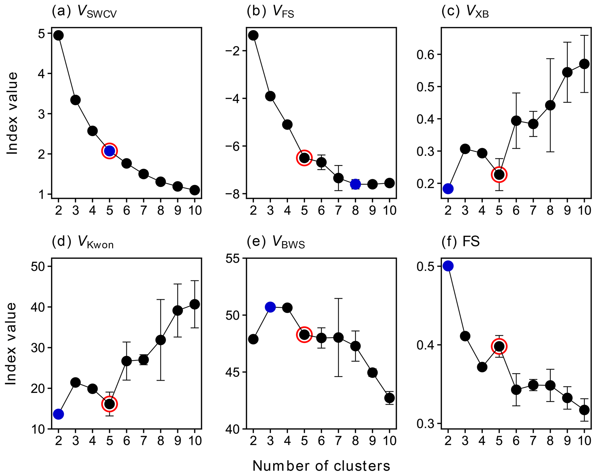
Figure 1 Values of selected clustering validity indices V_SWCV (a), V_FS (b), V_XB (c), V_Kwon (d), V_BWS (e), and FS (f) as a function of the number of clusters from 2 to 10. The averages of the results from 50 repetitions are shown in the plot, and the error bars show the standard deviations. Blue points denote the optimal values of c, according to each CVI, and the solution selected for further analysis is marked by red circles.

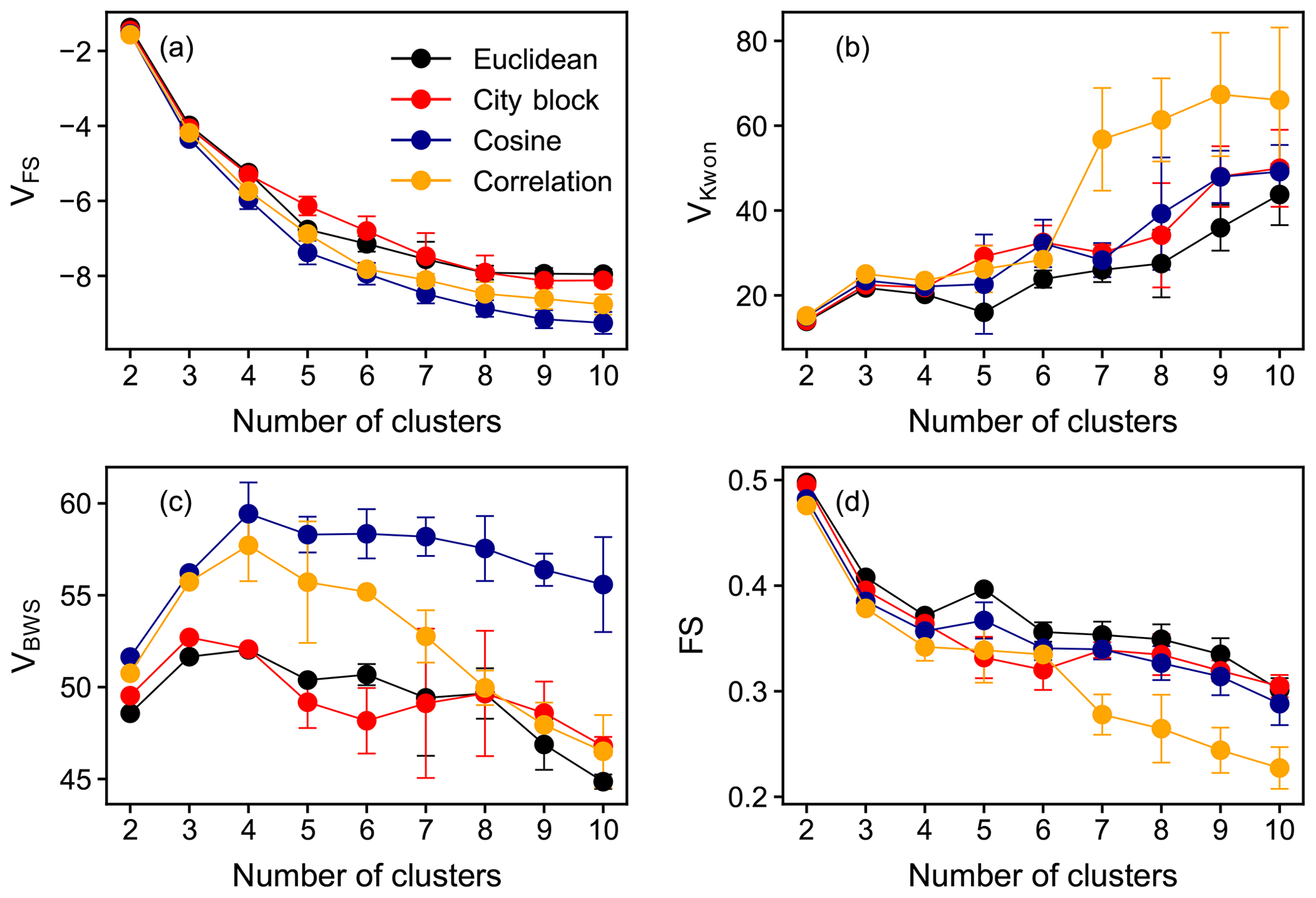
Figure 2 Values of selected clustering validity indices V_FS (a), V_Kwon (b), V_BWS (c), and FS (d) as a function of the number of clusters. Points in different colors are the results obtained with different distance or similarity metrics. The averages of results from 50 repetitions are shown in the plot, and the error bars denote the standard deviations. Euclidean distance was used in the calculation of CVIs.

In addition, the Bouguessa–Wang–Sun index (V_BWS) and the fuzzy silhouette values (FS​​​​​​​) were calculated for each FCM run. These two indices use slightly different definitions of compactness and separation to measure the quality of clustering. The V_BWS uses the fuzzy covariance matrix as a measure of compactness, and thus V_BWS takes the cluster shape, density, and orientation into account and has been proven to work well for largely overlapping clusters (Bouguessa et al., 2006; Bouguessa and Wang, 2004). In general, the larger the V_BWS, the better a fuzzy partition will be, and hence, the optimal number of clusters for our data is three (and four) based on V_BWS (Fig. 1e). Meanwhile, as depicted in Fig. 1e, V_BWS shows that there is a local optimum at c=7, though it has a higher uncertainty at this point. FS is an extension of the concept of the crisp silhouette (CS) that was originally developed to assess non-fuzzy clustering (Rousseeuw, 1987). It is more appealing than CS for fuzzy clustering, since it makes explicit use of the fuzzy partition matrix. In FS, objects in the near-vicinity of cluster centers are given more importance than those located in the boundary region (overlap). Consequently, it performs better than CS for highly overlapping data (Campello and Hruschka, 2006). In principle, a larger overall FS suggests a better partition. Therefore, the best number of clusters determined by FS is two (Fig. 1f). Nevertheless, when c=2, the sum of the within-cluster variance for this solution is still quite high (Fig. 1a), which is not expected for a good partition. It seems more sensible to set the number of clusters to five, as this is where FS reaches its local maximum and V_SWCV is significantly reduced and has the maximum curvature. It is worth noting that the silhouette score can not only be used to assess the overall quality of partition but also to evaluate the quality of individual clusters and objects. The silhouette score of an object ranges from −1 to +1, and a value close to +1 indicates that the object is correctly assigned. On the contrary, a silhouette value of −1 implies that the object is misclustered and should be assigned to a neighboring cluster. A silhouette value approaching zero suggests that the object is in the overlapping region of clusters, and thus the algorithm is unable to assign it to one cluster (Campello and Hruschka, 2006; Rawashdeh and Ralescu, 2012; Subbalakshmi et al., 2015).

In summary, different CVIs sometimes suggest a different optimal cluster number. However, by making use of information from multiple CVIs, the appropriate number of clusters in this study is determined to be five. It should be noted that the main topic of this study is to offer a proof of concept for the application of FCM in deconvolution of mass spectrometric data. Therefore, the depth of the discussion about the determination of the correct cluster number in this section must suffice for our purposes. The solution of c=5 is selected here as one example for the chemical characterization and kinetic parameterization in the following sections. In addition, It is worth mentioning that the multiple CVI method presented in this section provides a way to automatically determine the optimal number of clusters for FCM.

3.1.2 Distance metric

Figure 2 shows four selected CVIs as a function of c with different distance metrics. As mentioned before, smaller V_FS and V_Kwon indicate better partitioning, whereas for V_BWS and FS, the opposite applies. In terms of V_FS, it indicates that the cosine distance is more suitable for FCM in our case, although the impacts of different distance metrics on the clustering outcomes are minimal (Fig. 2a). The V_BWS values also suggest that the cosine distance is more appropriate for FCM regarding the data used in this study. As for V_Kwon and FS, there are no significant differences in the quality of partitioning when the number of clusters is small (e.g., c=2, 3, 4), despite different distance metrics, as shown in Fig. 2b and d. However, the discrepancies become more pronounced with increasing c. In general, the Euclidean distance is more appealing for our data in terms of V_Kwon and FS. To conclude, among all the examined distance metrics, the Euclidean and cosine distance provided a better performance in fuzzy clustering regarding the data used in this study, and the Euclidean distance was employed as the (dis)similarity metric in FCM for further analysis in this study. Additionally, the Euclidean distance was used in the calculation of various CVIs.

3.1.3 Fuzzifier value

Based on the fuzzy decision-making method introduced in Sect. 2.3.3, we searched m^∗ in the range of [1.1,9] with an increment of 0.1. The intersection of the fuzzy objective function, μ_G, and the fuzzy constraint, μ_C, as shown in Fig. 3a, indicates the optimal value of the fuzzifier for each run. To investigate whether m^∗ depends on c and U⁰, the number of clusters was set to vary from 2 to 10. For each c in this range, FCM was performed 50 times with a randomly created initial fuzzy partition matrix.

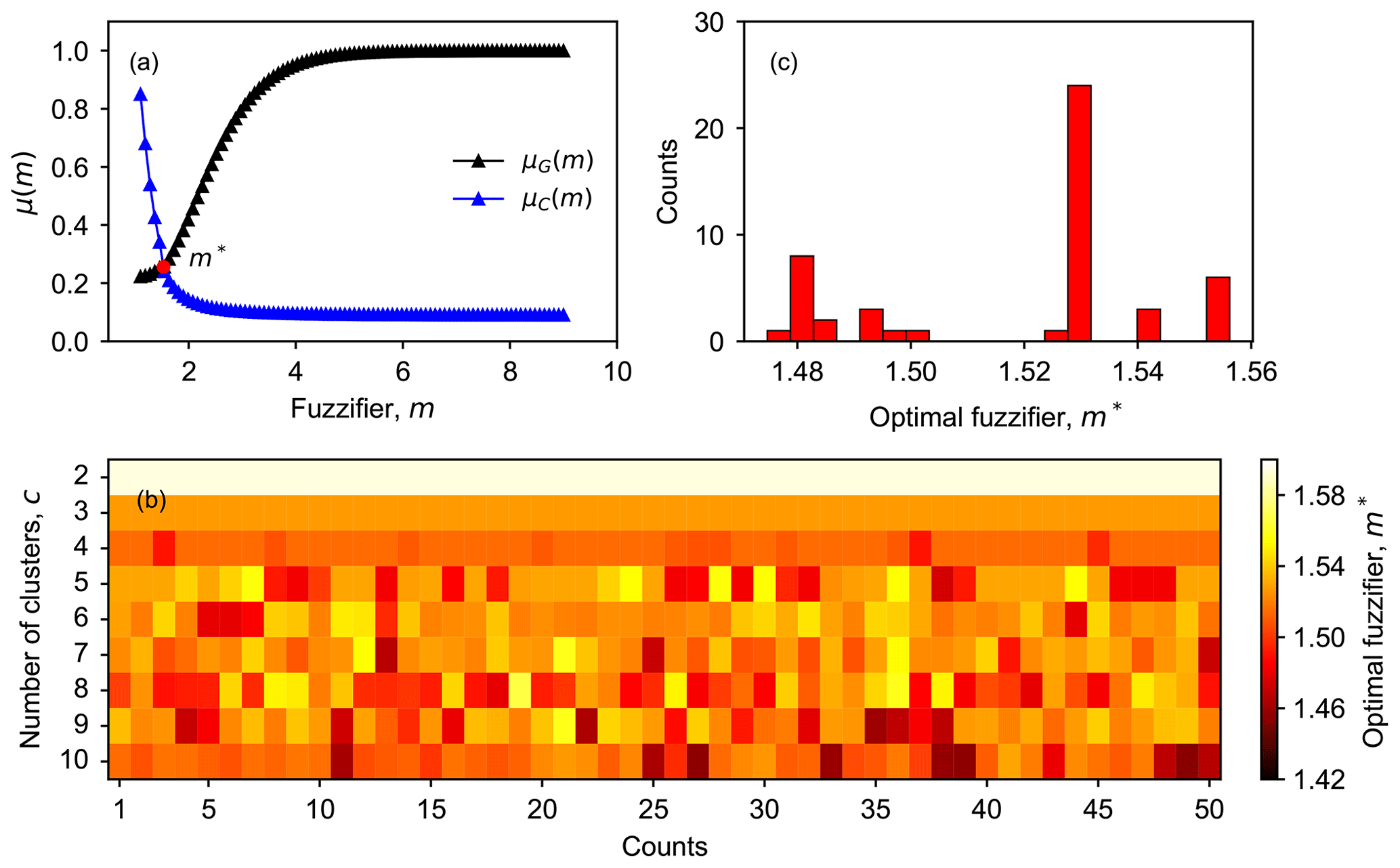
Figure 3 Determining the optimal value of the fuzzifier (m^∗) in FCM. In panel (a), the intersection (red point) of the fuzzy objective function (μ_G) and constraint (μ_C) is determined as m^∗. Panel (b) depicts the relationship between m^∗, the number of clusters (c), and the initial fuzzy partition matrix (U⁰). Panel (c) shows the frequency distribution of m^∗ for 50 repetitions with c=5 (determined as the optimal number of clusters in this study).

As shown in Fig. 3b, we do observe a relationship between m^∗ and $c/{\mathbf{U}}^{\mathrm{0}}$. For smaller cluster numbers, e.g., c=2 or 3, the determined optimal values of m are slightly larger than those obtained with larger c (c≥4). In addition, the results obtained with a smaller c are more robust. Different repetitions always return identical m^∗ values, suggesting that the initial fuzzy partition matrix does not affect m^∗ when the number of clusters is smaller than four. However, when c increases to four or even larger, then there is a variation in m^∗ among different repetitions, indicating that U⁰ starts to affect the determined value of m^∗, even though the variation in the value of m^∗ is small (between 1.42 and 1.52). One plausible explanation for the dependency of m^∗ on $c/{\mathbf{U}}^{\mathrm{0}}$ is shown as follows. When c is small, there are more overlaps between clusters, and thus m^∗ can be relatively large. When c becomes larger, the assignment becomes stricter, and the overlaps between clusters are reduced. Therefore, m^∗ gets smaller, and the clustering outcomes become more specific, which are likely to be more sensitive to local minima. Since the local minima largely depend on U⁰, consequently, the results become more sensitive to U⁰.

Figure 3c displays the distribution of m^∗ obtained from 50 repetitions with c=5. The histograms of the optimal value of m with other numbers of clusters are provided in the Supplement (Fig. S3). For c=5, the results suggest that the optimal value of m is 1.53 in most cases. Therefore, a value of m=1.53 is used for the FCM in this study.

Overall, the number of clusters and the initial membership degree matrix do affect the optimal value of the fuzzifier that was determined based on the fuzzy decision-making method in this study, but the influence is not very strong. The values of m^∗ determined for our dataset vary around 1.5, despite different c and U⁰, indicating that the FCM results in this study are relatively crisp.

3.2 FCM clustering results

3.2.1 FCM of chamber data

Using the appropriate clustering parameters determined in Sect. 2.3, we performed the transition from FCM to chamber data with the number of clusters varying from 2 to 10. For each c, the algorithm was run 50 times. According to the results of these 50 repetitions, two- and three-cluster solutions seem very robust. The repetitions always give identical outcomes, despite different initial partition matrices. This is also true for the five-cluster case. However, the influence of the initial position of the cluster centers on the partition increases when the number of clusters is further increased, but in all cases, more than half of the repetitions return the same results; thus, we select the most frequent outcomes as the final solutions for each case. Here we will not describe all solutions in detail but, instead, try to formulate a synthesis of the results and present the common features shared by solutions with different numbers of clusters.

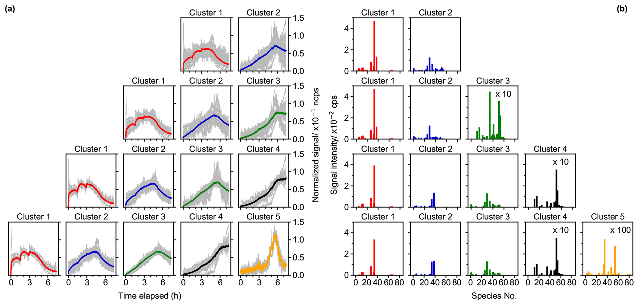
Figure 4 Results of fuzzy c-means clustering for chamber data with cluster numbers between two and five. Time series (a) and mass profiles (b) of clusters for each solution (in row). The time series of cluster centers are shown as thick colored solid lines, and the time series of species with the membership degree larger than 0.5 to the cluster are illustrated as thin gray lines. The species number in panel (b) corresponds to species listed in Fig. S7 (in order of molecular mass).

Figure 4 shows the FCM results with two to five clusters for the chamber data obtained during the isoprene–NO₃ experiment. Additional solutions with 6–10 clusters are shown in the Supplement (Fig. S4). Two distinct clusters emerge from the data in the two-cluster solution. According to their relative formation rates, cluster 1 is regarded as first-generation cluster, since species belonging to this cluster show a pronounced signal increase after the addition of the reactants, while cluster 2 behaves more like a second- or later-generation product, with its overall formation rate being much smaller than that of cluster 1. In addition to the time patterns, the mass profiles of cluster 1 and cluster 2 are clearly different (Fig. 4b).

When the cluster number is increased to three for both the time pattern and the mass profile of cluster 1, it almost remains unchanged compared to those in the two-cluster case. It seems that mainly the former cluster 2 is separated into two new clusters (clusters 2 and 3) with different formation rates for each. Cluster 2 is regarded as a representative of the second-generation processes, and cluster 3 represents third- or later-generation product, since it exhibits a smaller formation rate compared to cluster 2. However, there are fewer high-affiliation members (with a membership degree over 0.5) in cluster 1 in the three-cluster solution, indicating that at least some of the former contributors of this cluster have been moved, most likely to the new cluster 2. The mass profiles of cluster 2 and cluster 3 display quite distinct features, as shown in Fig. 4b, but the mass profiles of cluster 2 in both the two- and the three-cluster solution match to a large extent, even though their time patterns are somewhat different.

As shown in Fig. 4b, part of the species from cluster 1 in the three-cluster solution is separated out to a new cluster (cluster 2 in four-cluster solution) when increasing the number of clusters from 3 to 4. The newly formed cluster shares the same fingerprint molecules, i.e., C₅H₉NO₅ and C₅H₉NO₆ (corresponding to species nos. 34 and 38 in Fig. 4b), in the mass profile with cluster 1 in three-cluster case. This migrates the former cluster 2 into cluster 3 and cluster 3 into cluster 4, with some slight alterations in their time patterns and mass profiles. The time series of the new cluster 2 resembles that of cluster 1 but with smaller formation rates. In general, the member traces of different clusters seem to converge towards the time traces of the cluster centers, indicating that the system approaches the correct number of clusters.

When increasing the number of clusters from four to five, a new, distinct cluster (cluster 5) emerges, which has very small production in the early reaction stage, and its time trace shows that members in this cluster were destroyed significantly when there was abundant NO₃ in the system (step IV in Fig. S1). This specific character in time seems to already evolve in cluster 4 in the four-cluster solution. The mass profiles of the first four clusters of the five-cluster solution are very similar to those of the four-cluster case, but the mass profile of cluster 5 shows distinct differences from that of the others. It is important to mention that these five clusters now also effectively capture the loss rates over a timescale larger than 13 h and that most members in these clusters are well represented by their respective cluster centers.

When the number of clusters is further increased, more detailed and complicated clustering outcomes emerge, which is impelled by different formation and/or destruction pathways of species (Fig. S4). However, the differences between the new and existing clusters become smaller. Since the major objective of this study is to demonstrate the applicability of FCM in analyzing mass spectrometric data, we will not discuss the detailed interpretation of these solutions here.

To better understand the chemical composition of clusters, the bulk chemical properties like the hydrogen-to-carbon ratio (H : C), oxygen-to-carbon ratio (O : C), and average carbon oxidation state ($\stackrel{\mathrm{‾}}{{\mathrm{OS}}_{\mathrm{C}}}$) of different clusters were calculated and compared. The $\stackrel{\mathrm{‾}}{{\mathrm{OS}}_{\mathrm{C}}}$ of each cluster was calculated following the method proposed by Kroll et al. (2011), in which all the N atoms of N-containing compounds were assumed to be present in nitrate groups (and thus ${\mathrm{OS}}_{\mathrm{N}}=+\mathrm{5}$), as described in our previous study (Wu et al., 2021). Figure 5 shows the distribution of clusters in the $\stackrel{\mathrm{‾}}{{\mathrm{OS}}_{\mathrm{C}}}$ vs. n_C space for solutions with two to five clusters. Additional results for solutions with 6 to 10 clusters can be found in the Supplement (Fig. S5). The contribution of an individual species to a cluster is weighted by its nominal mass and signal intensity in the cluster profile. Regardless of the number of clusters, different solutions cover similar chemical composition ranges in terms of average $\stackrel{\mathrm{‾}}{{\mathrm{OS}}_{\mathrm{C}}}$ and n_C. However, there are discrepancies in detail. For example, the $\stackrel{\mathrm{‾}}{{\mathrm{OS}}_{\mathrm{C}}}$ of cluster 5 in the five-cluster solution slightly deviates from the trend that the other four clusters follow. A similar behavior is observed for cluster 1 in the six-cluster solution. This indicates that increasing the number of clusters could help to find new groups of species with distinct chemical compositions. However, further increasing the number of clusters to seven or more clusters does not yield new clusters with significantly different chemical composition, implying that c=5 or c=6 is the appropriate number of clusters in terms of separation by chemical composition. It is also shown in Fig. 5 that different clusters are well separated in the $\stackrel{\mathrm{‾}}{{\mathrm{OS}}_{\mathrm{C}}}$ vs. n_C space, despite some overlaps, indicating that they have distinct chemical compositions. For instance, the two early-generation clusters, cluster 1 and cluster 2 in the four-cluster solution, are differentiated from each other by their chemical properties.

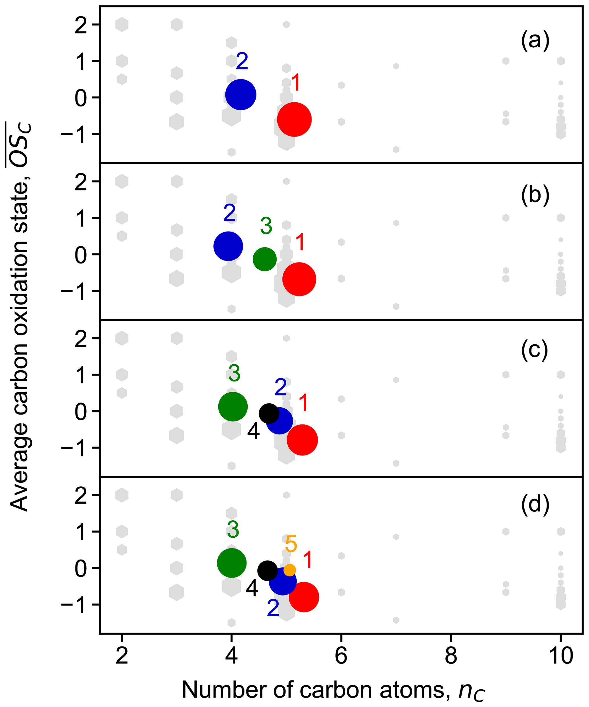
Figure 5 Average carbon oxidation state ($\stackrel{\mathrm{‾}}{{\mathrm{OS}}_{\mathrm{C}}}$) of the obtained FCM clusters from chamber data as a function of number of carbon atoms (n_C). Panels (a) to (d) show results for solutions with two to five clusters, respectively. Cluster centers are depicted by circles in different colors. The color scheme follows that in Fig. 4. The marker area of clusters is proportional to the sum of average signal intensity of all species in the cluster weighted by their membership degrees. Closed-shell products detected by Br⁻ CIMS are shown as gray hexagons, and the marker area is proportional to the average intensity of species over the whole experiment.

In general, the early-generation clusters with a lower oxidation degree fall in the corner of the plot with smaller $\stackrel{\mathrm{‾}}{{\mathrm{OS}}_{\mathrm{C}}}$ but larger n_C, while the later-generation clusters with a higher oxidation degree move towards the corner with larger $\stackrel{\mathrm{‾}}{{\mathrm{OS}}_{\mathrm{C}}}$ but smaller n_C. This indicates that the later-generation products detected in the gas phase in this study were formed through further oxidation of early-generation species and that they underwent more fragmentation during oxidation. Of course, it is very likely that there are later-generation products with larger n_C. However, as they become highly functionalized through multiple oxidation steps, they would have a very or extremely low volatility and thus mostly exist in the particle phase and be undetectable in the gas phase.

3.2.2 FCM of model data

As mentioned earlier, we also applied FCM to data obtained from a box model, with the default gas phase reaction schemes for isoprene–NO₃ taken from MCM v3.3.1 (Jenkin et al., 2015). For consistency, only closed-shell products from isoprene oxidation in MCM were taken for the clustering. Since the reaction scheme of isoprene with NO₃ in the MCM mechanism is semi-explicit, the clustering results of modeled data provide a way to evaluate the applicability of fuzzy clustering in analyzing time series data. In turn, by comparing the cluster centers derived from model data with those derived from mass spectrometric data, one can check if the model can reproduce the measurements well and thus investigate the representativeness of oxidation mechanism coupled in the model.

Figure 6 shows the results of FCM applied to model data, again with the number of clusters varying from two to five. It is clearly shown that different species are sorted according to their patterns of time behaviors and that different clusters represent multi-generation products. Taking the two-cluster solution as an example, the signals of most species in cluster 1 evidently increase as soon as the reaction is initiated, while those in cluster 2 grow considerably slow, indicating that cluster 1 is a surrogate of early-generation products, whereas cluster 2 corresponds to later-generation products. This is very similar to what we observe from the real measurements, even though the time behavior derived from those two cases is not the same. However, the fast-forming pathways play a more important role in the measured data than in the model data. In addition, more later-generation clusters are selected out from the model data with an increasing number of clusters, while the changes in early-generation clusters are indistinct. However, in terms of clusters 3–5 in the five-cluster solution, it is evident that certain chemical loss processes are missing from the MCM mechanism, which are observed from the chamber data. For instance, autoxidation and related processes for the isoprene–NO₃ system are underrepresented in the MCM, as well as the formation of accretion products.

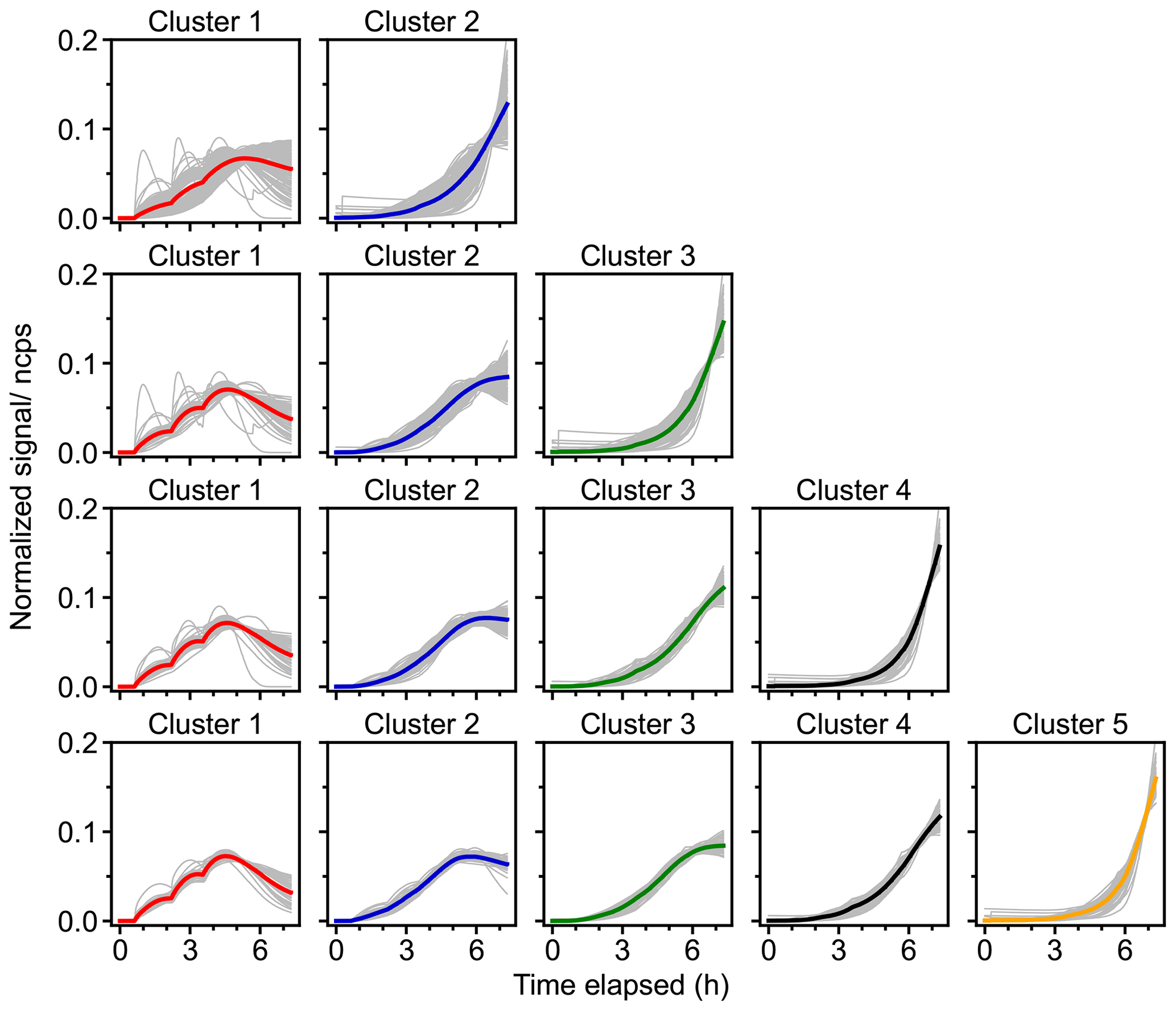
Figure 6 Results of FCM for model data with the number of clusters varying from two to five. Each row represents one solution, with the time series of cluster centers shown in solid thick colored lines, and the species with the membership degree larger than 0.5 to the cluster illustrated as solid thin gray lines.

As for the chemical properties, different clusters are discrete in the $\stackrel{\mathrm{‾}}{{\mathrm{OS}}_{\mathrm{C}}}$ vs. n_C space (Fig. S6), and thus it can be inferred that product species would also be grouped in a reasonable way when applying FCM to experimental data. Moreover, clusters in different solutions cover a similar chemical composition range of $\stackrel{\mathrm{‾}}{{\mathrm{OS}}_{\mathrm{C}}}$ and n_C despite increasing the number of clusters (except for the two-cluster solution), which is consistent with what we observed for the chamber data. However, the increase in the $\stackrel{\mathrm{‾}}{{\mathrm{OS}}_{\mathrm{C}}}$ of clusters for model data is less pronounced during the oxidation processes, probably due to the absence of autooxidation steps in the MCM. Moreover, the MCM lacks accretion products (mostly assigned to early-generation clusters with more carbon atoms in bulk) but tends to have more small species (with low n_C), which is not observed in the mass spectra data. This can be due to the detection limits of the Br⁻ CIMS for smaller compounds. Regarding the two-cluster solution, the chemical range of clusters is much narrower, and they are overlapping in the chemical space to some extent, suggesting that the number of clusters is not enough.

According to the outcomes from the application of FCM to both the measured and model data, we conclude that FCM can give interpretable and chemically meaningful results when it is applied to mass spectrometric data in a time series analysis.

3.3 Insights from clustering results

3.3.1 Chemical properties of different clusters

In this section, we utilize the five-cluster solution, identified as the optimal cluster number for our dataset (Sect. 2.3), to illustrate how to extract chemical and kinetic information from the mass spectrometric data based on the FCM analysis. This does not necessarily mean that the five-cluster solution is superior over others. However, as demonstrated in previous sections, the FCM results exhibit consistent features regardless of the number of clusters predefined. Therefore, findings derived from the five-cluster solution could potentially apply to other cases.

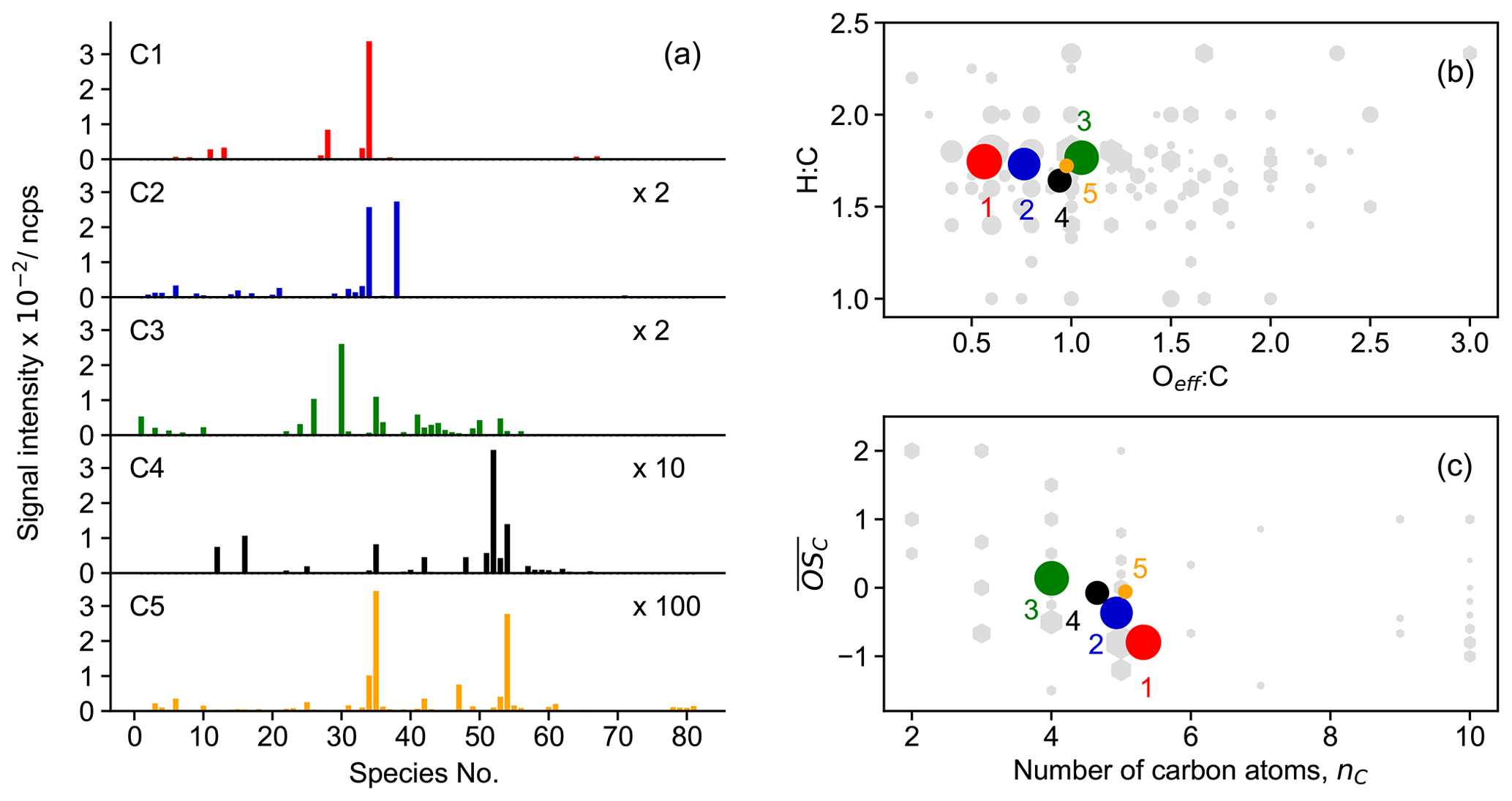
Figure 7 Chemical properties of clusters from the five-cluster solution. The subplots show mass profile of each cluster (a), van Krevelen plot (b), and average carbon oxidation state of clusters (c), respectively. Different clusters are distinguished by color, and the color scheme follows the one in Fig. 4. The marker area of the clusters is proportional to the sum of average signal intensity of all species in the cluster weighted by their membership degrees. The species number in panel (a) corresponds to species listed in Fig. S7 (in order of molecular mass). Gray hexagons in panels (b) and (c) denote species identified by Br⁻ CIMS, and the marker area is proportional to the average intensity of species over the whole experiment.

It is clearly shown in Fig. 7a that different clusters have significantly different compositions. For example, cluster 1, which represents the early-generation products, is dominated by a single species (with the chemical formula C₅H₉NO₅), and its intensity is much higher than those of the other four clusters. Another characteristic of cluster 1 is that more than 80 % of the detected 2N dimers (except one species with the formula C₁₀H₁₆N₂O₁₁) are assigned to this cluster (Fig. S7). These compounds are obviously first-generation products probably formed through RO₂ + RO₂ reactions (Wu et al., 2021). Therefore, it is reasonable to sort them into cluster 1, which is representative of the early-generation products. Cluster 2 also behaves like the early-generation products but differs from cluster 1 in terms of reactivity, i.e., formation and destruction rates. The differences in the cluster 1 and cluster 2 in chemical composition are even more perceptible. As shown in Fig. 7a, besides C₅H₉NO₅, there is another 1N monomer (C₅H₉NO₆) present in cluster 2 with a relatively high intensity. In addition, most of the detected small molecules (C_≤3) are assigned to this cluster (Fig. S7). Note that the formation rate of cluster 2 (from FCM analysis of the chamber data) resembles that of cluster 1 (in the five-cluster solution) from the FCM analysis of the model data. In addition, the fractions of some 3N dimers (e.g., C₁₀H₁₇N₃O_12–14) in cluster 2 are relatively high (Fig. S7). The 3N dimers are expected to be second- or even later-generation products that are produced from the cross-reaction of a first-generation nitrooxy peroxy radical and a secondary dinitrooxy peroxy radical or from further oxidation of the corresponding 2N dimers (Wu et al., 2021). This indicates that cluster 2 is very likely a mixture of the first- and second-generation products, which have not been resolved by the FCM in the five-cluster solution. Increasing the number of clusters might help to separate the typical behavior of a minority of components. When the cluster number is increased to six, it is indeed mainly the former cluster 2 in the five-cluster solution which is further split into new clusters (cluster 2 and cluster 3) in which the first-generation behavior of the new cluster 2 is more pronounced. From this point of view, the six-cluster solution seems better than the five-cluster solution.

Regarding later-generation clusters, namely cluster 3, cluster 4, and cluster 5, the second- or later-generation products, such as C₄ species and 2N and 3N monomers, are predominant in their composition. Nevertheless, the mass profiles of cluster 3, cluster 4, and cluster 5 are quite distinct. For example, cluster 3 is dominated mainly by a C₄ species (C₄H₇NO₅), while the major fingerprint of cluster 4 is constituted by two 2N monomers (C₅H₈N₂O₈ and C₅H₈N₂O₉), a C₄ species (C₄H₇NO₆), and a C₂ species (C₂H₃NO₅). In addition, 3N monomers are almost completely present in cluster 4 (Fig. S7). Cluster 5 has a much lower intensity compared to other clusters, and a distinctive characteristic of this cluster is a high contribution of two 3N dimers (C₁₀H₁₇N₃O₁₅ and C₁₀H₁₇N₃O₁₆) (Fig. S7).

Figure 7b and c show the chemical properties of each cluster center in terms of the bulk elemental molar ratios (in the van Krevelen space) and the average carbon oxidation state. The van Krevelen plot visualizes the chemical composition of organics by the hydrogen-to-carbon (H : C) vs. oxygen-to-carbon (O : C) ratio, and it is widely used to trace the origin and evolution of organic compounds (Chhabra et al., 2011). When calculating the O : C ratios of the N-containing compounds, the concept of effective oxygen number (n_{O_eff}, $n_{\mathrm{O}\mathrm{\_}\mathrm{eff}}=n_{\mathrm{O}}-\mathrm{2}\times n_{\mathrm{N}}$) was employed, whereas in the case of a nitrate group, only one of the O atoms bonded to C atom was considered in the calculation (Xu et al., 2021). The cluster centers cover a narrow range of chemical space of the original dataset (gray circles in Fig. 7b) but are located where most of the compounds fall in. They lie almost along a line of H : C = 1.75 in the van Krevelen plot, indicating that they have gained on average one H atom compared to isoprene. A trajectory with a slope of zero is expected in van Krevelen plots when only alcohol or hydroperoxide functionalities are introduced in the molecule (Chhabra et al., 2011). This is a characteristic of autoxidation steps (–OOH) or H shifts in alkoxy radicals (−OH and thereafter −OOH). Therefore, the distribution of the clusters in the van Krevelen space implies that autoxidation steps or intramolecular H shifts were involved in the reactions of isoprene with NO₃ studied in this work.

In terms of average oxidation state and carbon atom numbers, the early-generation products which undergo fewer oxidation steps usually have a much lower oxidation degree but more carbon atoms per molecule. With the reaction proceeding, the early-stage products will be further oxidized and fragmented, leading to the formation of later-generation products with a higher oxidation state but less carbon atoms per molecule. Consequently, the trajectory of chemical processes generally starts with the precursor in the lower-right corner and moves towards to the upper-left area (products) in the ${\stackrel{\mathrm{‾}}{\mathrm{OS}}}_{\mathrm{C}}$ vs. n_C space through oxidation and fragmentation. In this study, the early-generation clusters have a lower oxidation state but more carbon atoms, while the later-generation clusters are the other way around, thus following the oxidation trajectory in chemical space well.

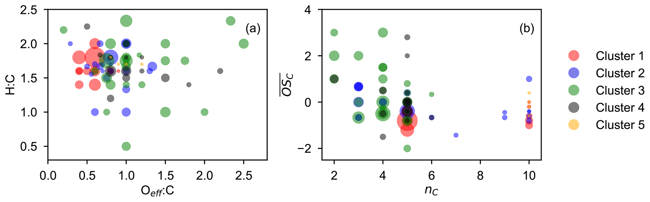
Figure 8 Chemical properties of high-affiliation species from each cluster (with a membership degree larger than 0.5) described by van Krevelen (a) and average carbon oxidation state ($\stackrel{\mathrm{‾}}{{\mathrm{OS}}_{\mathrm{C}}}$) vs. carbon number (n_C) (b) plot. The marker area is proportional to the average signal intensity of species over the whole experiment.

When considering the characteristics of members in each cluster, we focus solely on high-affiliation species (with a membership degree over 0.5) to simplify the discussion. Figure 8 shows the chemical properties of the high-affiliation species described by their elemental molar ratios and average carbon oxidation state. In general, most of the high-affiliation species of the two early-generation clusters (clusters 1 and 2) center in a relatively low O_eff : C area of the van Krevelen plot, while those from the three later-generation clusters (clusters 3, 4, and 5) spread to the higher O_eff : C area. This confirms that species belonging to later-generation clusters are generally more oxidized than those from early-generation clusters, as expected. With respect to the average oxidation state, species of cluster 1 in general have lower ${\stackrel{\mathrm{‾}}{\mathrm{OS}}}_{\mathrm{C}}$ than others, and they are mainly monomers (n_C = 5) and dimers (n_C = 10). The ${\stackrel{\mathrm{‾}}{\mathrm{OS}}}_{\mathrm{C}}$ of species from cluster 2 is slightly higher than that from those of cluster 1, and there are more fragments in this cluster, including both monomers with n_C < 5 and dimer species with 5 < n_C < 10. The high-affiliation species of later-generation clusters generally have a higher oxidation degree than that from early-generation clusters but most of them are molecules with fewer than six carbon atoms.

Based on abovementioned results, we conclude that FCM is a feasible dimension reduction technique for dealing with complex mass spectrometric data from an oxidation system of interest. The derived clusters show a chemically realistic time behavior and cover the major range of the chemical properties of the original dataset. This suggests that the FCM could be useful for the simplification and analysis of mass spectra data and that the chemical information underlying in the clusters can be helpful for understanding the system of interest.

3.3.2 Kinetic properties of different clusters

The FCM results show that different clusters have different time behaviors, indicating that they were formed by different (or a series of) reaction steps. By fitting the GKP function (Eq. 12) to the measurements, we can extract underlying kinetic information (effective rate constant k and generation number m_G) from time series data. Generally, a larger value of k implies a faster formation rate of a product class for a given oxidant exposure, and vice versa. It should be noted that the k obtained here is not a stepwise rate constant, and it has no direct relationship with the stepwise rate constants of the reaction sequence. However, this value offers a way to quantitatively measure the overall rate constant of all reactions along the pathway (Koss et al., 2020). Since the FCM cluster centers represent chemically realistic time patterns and retain the major kinetic properties of the original dataset, they can be used as surrogates for various products formed in the isoprene–NO₃ system, and the GKP function can be fitted to the time series of cluster centers. This largely reduces the complexity of the data analysis and provides a way to get kinetic information directly from measurements.

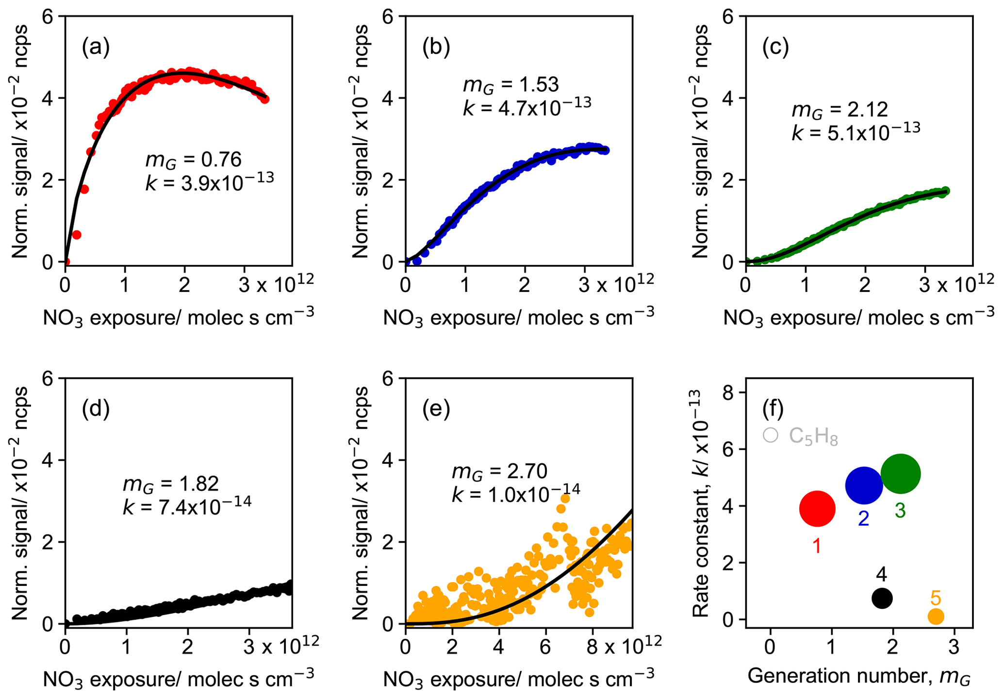
Figure 9 Parameterized effective rate constant (k; cm³ molec.⁻¹ s⁻¹) and generation number (m_G) for FCM clusters (five-cluster case) derived from CIMS measurements of isoprene–NO₃ system. Panels (a) to (e) show the GKP fitting results for different clusters, with cluster 1 in red, cluster 2 in dark blue, cluster 3 in green, cluster 4 in black, and cluster 5 in orange, respectively. Colored dots in each panel are the time series of the clusters, and black lines are GKP fits. Panel (f) shows the distribution of the kinetic parameters. The marker area is proportional to the sum of average intensity of all species in the clusters weighted by their membership degrees.

Figure 9 shows the result of the fit of GKP to the FCM clusters derived from the chamber measurements for the five-cluster solution. All except cluster 5 are fitted with a coefficient of determination (r²) of 0.96 or higher, indicating that the GKP model can reproduce the kinetic behavior of the products formed from the isoprene–NO₃ oxidation system in this study well. Cluster 5 is not well reproduced (with a r² of 0.41), probably due to its extremely low and noisy signal as a surrogate of the later-generation products. The fitted values of m_G for early-generation clusters are expected to be one (in theory). As depicted in Fig. 9a, the generation number of cluster 1 is close to one and that of cluster 2 is between one and two, coinciding with the expectation. As for the three later-generation clusters, their m_G values are approximately two (clusters 3 and 4) or three (cluster 5), indicating that they undergo two or more NO₃ oxidation steps.

There are several possible reasons for non-integer values of m_G, including uncertainties from signal noise, especially for low signal-to-noise data, and possible influences from physical processes like vapor–wall interaction, which can lower the signal of species and thus lead to a higher fitted m_G (Koss et al., 2020). In addition, the value of m_G can be distorted to some extent if compounds are produced from isoprene oxidation by oxidants other than NO₃, e.g., OH and O₃, in this case. While NO₃ makes up the major fraction of consumption of isoprene, its reactions with O₃ and OH still contribute 10 %–15 % of the isoprene loss (Vereecken et al., 2021; Carlsson et al., 2023). Consequently, it is very likely that some species detected by CIMS were oxidized by multiple oxidants. Such an effect will lower m_G, as unaccounted sources increase the concentrations of species besides the NO₃ exposure, and the linear, first-order kinetic assumption of the GKP model is no longer applicable. For example, the isoprene hydroperoxy aldehyde (C₅H₈O₃), one of the major products from photooxidation, is also observed from NO₃-initiated oxidation (Vereecken et al., 2021; Wennberg et al., 2018; Wu et al., 2021). Furthermore, the deviation of m_G from integer values can occur if isomers that were formed by a different number of oxidation steps exist.

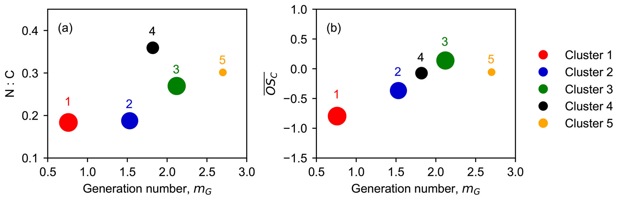
Figure 10 Relationship between generation number (m_G) and chemical properties of clusters. Nitrogen-to-carbon (N : C) ratio (a) and average carbon oxidation state ($\stackrel{\mathrm{‾}}{{\mathrm{OS}}_{\mathrm{C}}}$) (b) as a function of m. The marker area is proportional to the sum of average intensity of all species in the clusters weighted by their membership degrees.

Since the generation number corresponds to the reaction steps with NO₃ to form the product, the later-generation species, which undergo more oxidation steps, should have larger m_G values and higher nitrogen-to-carbon ratios (N : C) when considering that NO₃ is the only oxidant. Figure 10 shows the relationship between generation number and chemical properties of clusters. In general, clusters with higher m_G have larger N : C ratios, as expected, confirming that NO₃ is the predominate oxidant for isoprene oxidation in our system. Nonetheless, we find that species with larger N : C ratios are not necessarily later-generation products. As shown in Fig. 9a, cluster 4 has a larger N : C ratio than cluster 3 and cluster 5, but it appears with a smaller m_G. This indicates that some of the nitrogen atoms of compounds in cluster 4 were gained through non-oxidative steps. On the other hand, cluster 5 has a larger m_G value than cluster 3 and cluster 4, but its N : C ratio is relatively small. This is probably because the species in cluster 5 were formed by isoprene oxidation by other oxidants than NO₃, e.g., OH and O₃. Another plausible explanation could be that the NO₃ oxidation reaction does not lead to an increase in nitrogen content in the product molecules, e.g., through H abstraction instead of the addition to C=C double bonds (Wu et al., 2021).

There is a strong linear correlation between the generation number and the average oxidation state of the clusters, apart from cluster 5, as illustrated in Fig. 10b. The early-generation clusters have smaller m_G values than later-generation clusters, which corroborates that the generation number returned by the GKP model is reasonable. The linear regression result shows that the value of $\stackrel{\mathrm{‾}}{{\mathrm{OS}}_{\mathrm{C}}}$ increases by ∼ 0.74 for each generation. For m_G = 0, the corresponding $\stackrel{\mathrm{‾}}{{\mathrm{OS}}_{\mathrm{C}}}$ is −1.45, approximate to the average carbon oxidation state of isoprene ($\stackrel{\mathrm{‾}}{{\mathrm{OS}}_{\mathrm{C}}}=-\mathrm{1.6}$). For each addition of NO₃ functionality, the $\stackrel{\mathrm{‾}}{{\mathrm{OS}}_{\mathrm{C}}}$ of the corresponding product increases by 0.2, and the following O₂ addition (if possible) results in the $\stackrel{\mathrm{‾}}{{\mathrm{OS}}_{\mathrm{C}}}$ increasing by additional 0.8. Therefore, it involves at least one autooxidation step for each NO₃ addition, considering an increase of about 0.8 in $\stackrel{\mathrm{‾}}{{\mathrm{OS}}_{\mathrm{C}}}$ per generation.

Cluster 5 has a m_G value approaching three, suggesting that the species belonging to this cluster underwent roughly three oxidation steps. However, its average oxidation rate is unexpectedly low, deviating from the linear line of m_G and $\stackrel{\mathrm{‾}}{{\mathrm{OS}}_{\mathrm{C}}}$. One plausible explanation for this is that such species are probably formed through unimolecular fragmentation. For example, if the H abstraction (of RO₂) occurs at a carbon with an −OOH functionality attached, the reaction chain will be terminated by an OH loss and lead to the formation of a carbonyl compound (Bianchi et al., 2019), which results in products with a lower average oxidation state.

In general, the effective rate constants of the clusters are limited by the reaction rate constant of isoprene, and the early-generation clusters have larger k values than the later-generation ones. As shown in Fig. 9f, the returned k values of the two early-generation clusters 1 and 2 are very close to the reaction rate constant of isoprene with NO₃ (6.5 × 10⁻¹³ cm³ molec.⁻¹ s⁻¹ at 298 K, IUPAC, https://iupac-aeris.ipsl.fr/datasheets/pdf/NO3_VOC8.pdf, last access: 15 March 2024). The k values of the later-generation clusters, clusters 4 and 5, are about 1 order of magnitude smaller. Cluster 3, which represents second-generation products with m_G≈2, has a similar effective rate constant to cluster 1 and cluster 2, indicating that the species belonging to this cluster form or react relatively fast. As shown in Fig. 7c, cluster 3 has a high oxidation degree but fewer carbon atoms on average, suggesting that the species in cluster 3 are probably highly oxidized fragments. This is confirmed by its mass profile (Fig. 7a).

The GKP method was also applied to individual species. Examples of fits for various species are shown in Fig. S8. Figure 11 depicts the fitted k and m_G values of the high-affiliation species from each cluster. For species from cluster 1, cluster 2, and cluster 3, most of the returned k values fall into the same order of magnitude to the rate constant of isoprene with NO₃ (k = 6.5 × 10⁻¹³ cm⁻³ molec.⁻¹ s⁻¹ at 298 K). For those from the two later-generation clusters, clusters 4 and 5, the returned k values are about 1 and 2 order(s) of magnitude smaller, respectively. Most returned m_G of species from cluster 1 are around one, indicating that they are formed after one oxidation step (with NO₃), which is consistent with the expectation for early-generation products. However, the returned m_G of some species from cluster 1 are between one and two, e.g., the compound(s) with the formula of C₅H₉NO₅ (the largest red marker in Fig. 11). This suggests that such species may consist of isomers originating from more than one pathway with different number of oxidation steps.

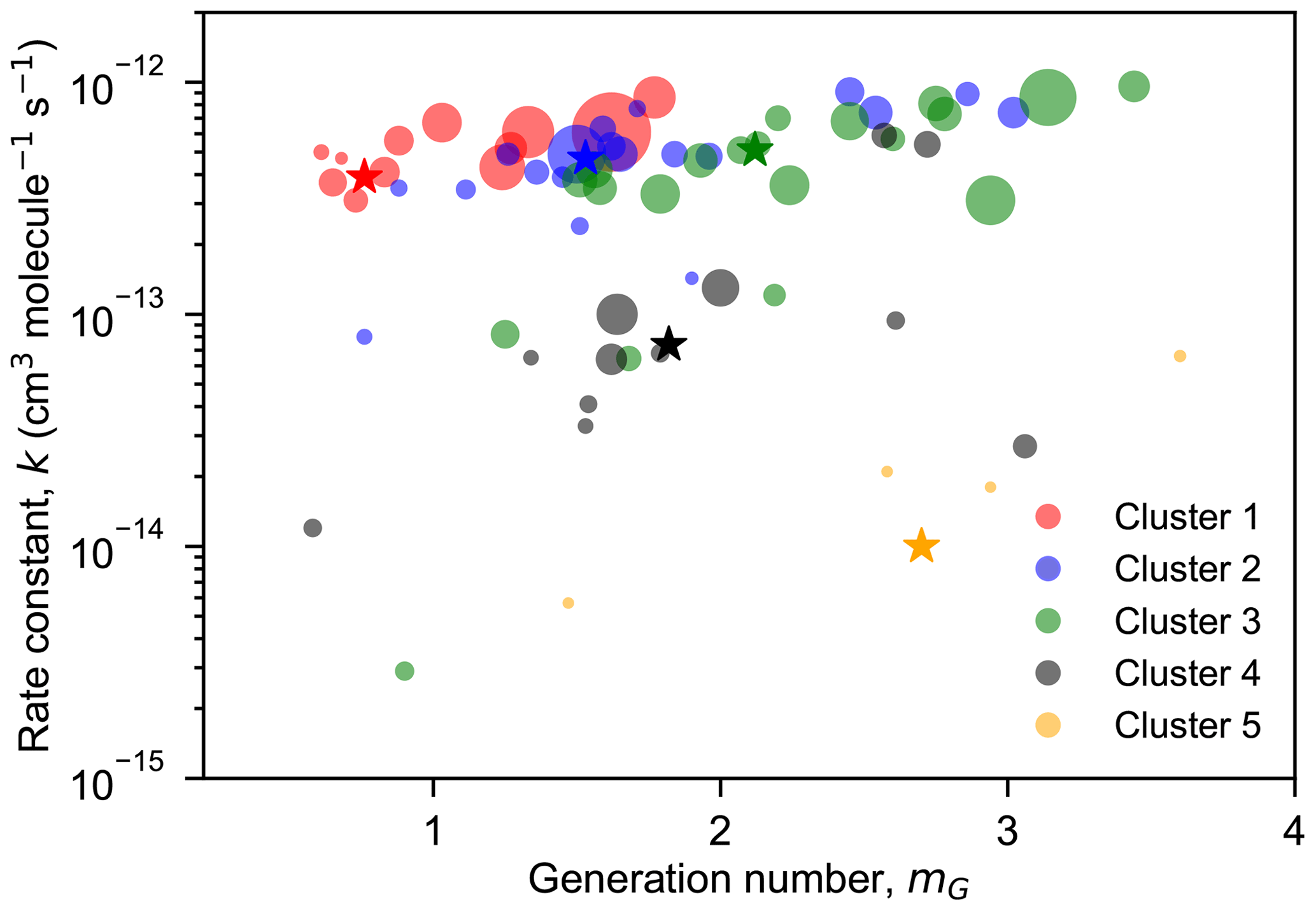
Figure 11 Fitted effective rate constant (k) and generation number (m_G) of the high-affiliation species of each FCM cluster. The cluster centers and members are denoted by color-coded circles and pentagrams, respectively. The circle area is proportional to the average signal intensity of species over the whole experiment.

For species belonging to cluster 2, their m_G are mostly in a range from one to two, but there are also some smaller molecules (mainly C₃ and C₄ species) with larger m_G values, indicating that such fragmented compounds are formed after multiple oxidation steps. With regard to species from later-generation clusters, the returned m_G values span a broader range, but there are no compounds with a generation number larger than four. In general, most of the high-affiliation species (from both the early- and later-generation) fall in the fast-reacting (large k) area, with a few of exceptions having relatively small k and m_G. These two types of compounds are both kinetically realistic. However, there are several species with large m_G (around three) but relatively small k, e.g., C₁₀H₁₇N₃O₁₅ and C₁₀H₁₇N₃O₁₆ from cluster 5. This suggests that they are slow-forming products that appear after several oxidation steps, which should be difficult to form and thus should be low in signal or even undetectable. In fact, the signals of C₁₀H₁₇N₃O₁₅ and C₁₀H₁₇N₃O₁₆ are extremely low and noisy at the beginning of the reaction, as shown in Fig. S8u and v. Detectable increases in the signal of these masses are only observed when the NO₃ exposure was relatively high.

To conclude, the kinetic parameters derived from GKP fitting to the clusters are reasonable and well correlated to their chemical properties. Specifically, isoprene products formed in the early stage are larger molecules but less oxidized and with relatively high reactivity, while those formed in the later stage tend to be smaller but highly oxidized and less reactive. Fragmented species are exceptions that have a relatively high oxidation degree and are simultaneously reactive.

3.4 Implications for isoprene–NO₃ chemistry

As noted previously, one big advantage of FCM is that variables can be affiliated to multiple clusters, which relates to many real-world problems in a more realistic and reasonable way. It is explained in Sect. 3.3 that different FCM clusters have distinct differences in chemical and kinetic properties, potentially representing different chemical processes. Therefore, the clustering distribution of a species gives an insight into its formation mechanism.

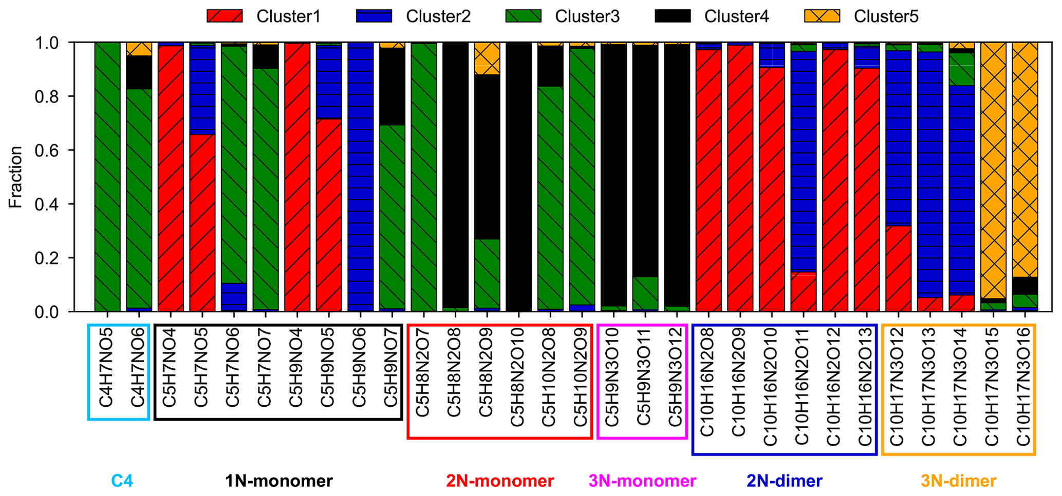
Figure 12 Cluster apportionment of selected major products from the isoprene–NO₃ oxidation system. The colored boxes correspond to different types of products.

Figure 12 shows the cluster apportionment of selected major products formed from isoprene oxidation by NO₃. Since different FCM clusters represent different types of chemical processes or products that have distinct chemical and kinetic properties, a different distribution indicates different formation pathways of the respective species. According to the general reaction scheme of isoprene with NO₃ (scheme S1), 1N and 2N monomers are expected to be the first- and second-generation products, respectively. The accretion products are supposed to be formed from the RO₂ + RO₂ reaction (Berndt et al., 2018), and thus 2N dimers are probably originating from the self- or cross-reactions of two C₅-nitrooxy peroxy radicals, while 3N dimers are most likely produced by cross-reactions of C₅​​​​​​​ nitrooxy peroxy radicals with C₅ dinitrooxy peroxy radicals (Ng et al., 2008; Wu et al., 2021). Accordingly, 2N and 3N dimers should be first- and second-generation products, respectively. A possible permutation scheme for the formation of 2N and 3N dimers can be found in Table S1 in the Supplement.

The FCM results affirm these suppositions to some extent. For example, 1N monomer species like C₅H₉NO₄ and C₅H₉NO₅ are predominant in early-generation clusters (cluster 1 and cluster 2), while 2N monomers are mostly found in the later-generation clusters (cluster 3 and cluster 4). However, there are some exceptions, such as C₅H₇NO₆ and C₅H₇NO₇. These two species have entirely different cluster distributions compared to C₅H₇NO₄ and C₅H₇NO₅, regardless of their similar formula composition. The majority of C₅H₇NO₆ and C₅H₇NO₇ is apportioned to the second-generation cluster (cluster 3), indicating that C₅H₇NO₆ and C₅H₇NO₇ are second-generation products, whereas C₅H₇NO₄ and C₅H₇NO₅ are subsumed in early-generation products. A similar phenomenon is observed among C₅H₉NO₇, C₅H₉NO₄, and C₅H₉NO₅. Another example is the 3N dimers. In theory, 3N dimers are supposed to be second-generation products (Table S1), but the FCM outcomes show that different 3N dimers are formed from different pathways with different generations. For example, C₁₀H₁₇N₃O₁₂, C₁₀H₁₇N₃O₁₃, and C₁₀H₁₇N₃O₁₄ are supposed to be early-generation products, based on the FCM results, whereas C₁₀H₁₇N₃O₁₅ and C₁₀H₁₇N₃O₁₆ are supposed to be third- or even later-generation products that have much lower formation rates compared to typical secondary compounds. This implies that the formation mechanisms of 3N dimers are more complicated than expected. Further investigation is needed to understand distinct behaviors of different 3N dimers observed in this study.

In terms of 2N monomers, the clustering results confirm that they are very likely second-generation products, but some species probably originated from different formation pathways, even though they have the same generation number. As shown in Fig. 12, most fractions of C₅H₈N₂O₈ and C₅H₈N₂O₁₀ fall into cluster 4, whereas C₅H₈N₂O₇, C₅H₁₀N₂O₈, and C₅H₁₀N₂O₉ are primarily assigned to cluster 3. Cluster 3 and cluster 4 are different in their chemical and kinetic properties, as described in Sect. 3.3, which most likely represent two different chemical processes. A similar phenomenon is observed in C₁₀H₁₆N₂O₁₁, which has a distinctive distribution compared to other 2N dimers. This signifies the uniqueness of its formation mechanism.

Although a species can be apportioned to multiple clusters in FCM, most products in this study predominantly belong to one cluster, e.g., C₅H₉NO₄ and C₅H₉NO₆, suggesting that they were formed predominantly through a single pathway. In contrast, some species are primarily made up of two clusters, such as C₅H₇NO₅, C₅H₉NO₅, C₅H₉NO₇, and C₁₀H₁₇N₃O₁₂, indicating that they are probably comprised of two structural isomers or that they originate from two different reaction pathways (with different oxidation steps).

All of these findings from FCM are valuable and can be used as constraints for mechanism development, especially for less-known species. For example, C₄H₇NO₅ is ubiquitous in the atmosphere and contributes significantly to isoprene organonitrates, but it is less investigated (Tsiligiannis et al., 2022). Only a few studies mentioned the formation processes of C₄H₇NO₅ in daytime chemistry (Jenkin et al., 2015; Praske et al., 2015; Schwantes et al., 2015; Wennberg et al., 2018). The formation mechanism of this compound in the nighttime is unclear yet (Tsiligiannis et al., 2022; Wu et al., 2021). According to the FCM outcomes, C₄H₇NO₅ is exclusively assigned to cluster 3 (a second-generation cluster), suggesting that C₄H₇NO₅ is a second-generation product and is mainly originating from a single pathway. Combining this information together with its molecular composition, we proposed that C₄H₇NO₅ is probably formed via further oxidation of the hydroxy carbonyl (C₅H₈O₂) by NO₃, as shown in scheme S2 in the Supplement (Wu et al., 2021). In a recent publication, Tsiligiannis et al. (2022) have discussed the sources and fate of C₄H₇NO₅ based on both measurements and modeling results. They suggest that decomposition of C₅H₈NO₇ radicals, nitrated epoxides, or peroxides are also plausible formation pathways for nighttime C₄H₇NO₅. Nonetheless, the fuzzy clustering results suggest that there is only one major formation channel (or maybe an unknown pathway) for C₄H₇NO₅ detected in our system.

4 Conclusions

Recent advances in mass spectrometry, especially the development of CIMS, empower us to detect low-volatility vapors in the gas phase directly and largely enhance our understanding of the formation mechanism of SOA. However, the complex, highly resolved mass spectra introduce new difficulties for data processing and interpretation. Although different statistical analysis techniques, such as PMF, PCA, and HCA, have been proposed and widely used to analyze mass spectrometric data, the application of fuzzy clustering algorithms in analyzing CIMS data has not yet come into common view.

In this study, we promote adopting the FCM method for the analysis of CIMS data obtained from complex oxidation systems. Different from hard clustering algorithms, FCM allows variables to belong to multiple clusters, which is more suitable for overlapping data and more reasonable for measurements in atmospheric science.

Several parameters need to be defined before running FCM, such as the number of clusters, fuzzifier value, and the distance metric used for measuring dissimilarity, which have a critical effect on clustering outcomes. Using multiple clustering validity indices, the impacts of these parameters on the partition were evaluated, and their optimal values were determined for our dataset. Furthermore, based on a practical case, we exemplified the functionalities of FCM in understanding the chemical and kinetic properties of the investigated system.

Overall, the FCM approach we presented in this work is an applicable and useful tool to analyze mass spectrometric data. It largely simplifies the characterization of an oxidation system by grouping numerous products into a much smaller number of clusters, based on their different chemical and kinetic properties. The chemical and kinetic information retained from the clustering outcomes helps to understand the chemical processes involved in the investigated system and can be useful for mechanism development.