the Creative Commons Attribution 4.0 License.
the Creative Commons Attribution 4.0 License.
 | 23 Apr 2024
Large-scale automated emission measurement of individual vehicles with point sampling
Martin Penz
Hannes Juchem
Christina Schmidt
Denis Pöhler
Alexander Bergmann
Currently, emissions from internal combustion vehicles are not properly monitored throughout their life cycle. In particular, a small share of vehicles (< 20 %) with malfunctioning after-treatment systems and old vehicles with outdated engine technology are responsible for the majority (60 %–90 %) of traffic-related emissions. Remote emission sensing (RES) is a method used for screening emissions from a large number of in-use vehicles. Commercial open-path RES systems are capable of providing emission factors for many gaseous compounds, but they are less accurate and reliable for particulate matter (PM). Point sampling (PS) is an extractive RES method where a portion of the exhaust is sampled and then analyzed. So far, PS studies have been predominantly conducted on a rather small scale and have mainly analyzed heavy-duty vehicles (HDVs), which have high exhaust flow rates. In this work, we present a comprehensive PS system that can be used for large-scale screening of PM and gas emissions, largely independent of the vehicle type. The data analysis framework developed here is capable of processing data from thousands of vehicles. The core of the data analysis is our peak detection algorithm (TUG-PDA), which determines and separates emissions down to a spacing of just a few seconds between vehicles. We present a detailed evaluation of the main influencing factors on PS measurements by using about 100 000 vehicle records collected from several measurement locations, mainly in urban areas. We show the capability of the emission screening by providing real-world black carbon (BC), particle number (PN) and nitrogen oxide (NOx) emission trends for various vehicle categories such as diesel and petrol passenger cars or HDVs. Comparisons with open-path RES and PS studies show overall good agreement and demonstrate the applicability even for the latest Euro emission standards, where current open-path RES systems reach their limits.
- Article
(6253 KB) - Full-text XML
-
Supplement
(4815 KB) - BibTeX
- EndNote


Exhaust emissions from combustion-based vehicles are negatively affecting human health and our environment. Of specific interest are nitrogen oxide (NOx) and particulate matter (PM) emissions due to the known impact on health, the environment and the climate (Mannucci et al., 2015; EEA, 2017). NOx emissions remain a widespread problem, especially for diesel-powered vehicles, where tampered, defective and old vehicles are the main source of high emission levels (Meyer et al., 2023). For PM it is well known from the literature that a small share of vehicles (< 20 %) contribute to the vast amount (60 %–90 %) of emissions (Park et al., 2011; Burtscher et al., 2019; Boveroux et al., 2019; Bainschab et al., 2020). This is due to malfunctioning after-treatment systems, such as defective diesel particulate filters (DPFs) and old vehicles with degenerated or outdated technologies. It would be highly beneficial to human health and the environment if these high emitters could be identified and subsequently maintained to significantly reduce emissions. Most current regulations are only related to type-approval procedures, but they do not consider deterioration (e.g., of the exhaust after-treatment system), defects that are not properly repaired or tampering that occurs in the lifetime of the vehicles (Mock and German, 2015; Bainschab et al., 2020). Particle number (PN) and black carbon (BC) are two PM metrics of particular interest. In addition to its impact on health and the climate, BC is a suitable tracer for vehicles with high PM emissions (Salimbene et al., 2021; Rönkkö et al., 2023). Interest in real-world PN emissions is growing due to newly introduced regulations (Giechaskiel et al., 2021) and to the known health effects on the human respiratory and cardiovascular systems (Oberdörster et al., 2005; Brook et al., 2010).
Different strategies try to address these issues. PN concentration measurements during periodic technical inspections are currently implemented in several European countries such as Germany, the Netherlands, Switzerland and Belgium. The PN inspections should identify malfunctioning vehicles during low-idle operation (Bainschab et al., 2020; Giechaskiel et al., 2020, 2021; Melas et al., 2021). A disadvantage of the periodic technical inspections is that they are in the best case annual, one-time measurements performed under non-real-driving conditions, which can potentially be circumvented by tampering or by manipulating measurements.
Another approach taken for high-emitter identification and the screening of real-world emissions of in-use vehicles is remote emission sensing (RES). RES is employed directly at the roadside to measure emissions from passing vehicles under real-driving operating conditions (Bishop et al., 1989; Borken-Kleefeld and Dallmann, 2018). One advantage of RES is that the vehicles are measured during their normal operation, which complicates fraud. Commercially available RES systems are open-path systems that detect the light extinction of the exhaust plume at different wavelengths to measure different pollutants emitted by passing vehicles (Bishop et al., 1989; Stedman et al., 1992; Moosmüller et al., 2003; Burgard et al., 2006). These systems deliver statistically acceptable emission factors (EFs) for gaseous species, but EFs are inaccurate for particulates. In particular, PM emissions of the latest Euro emission standards (Euro 6, Euro VI and beyond) are below the quantification limit of open-path RES systems (Gruening et al., 2019; Cha and Sjödin, 2022; Jerksjö et al., 2022). Other PM metrics such as PN or BC are not measured by these systems, as they only give PM mass emission estimates (Knoll et al., 2024). Complementary RES concepts exist which can be applied to counteract the downsides of these systems. In plume chasing, a measurement vehicle equipped with laboratory-grade analyzers traces the vehicles under test. Several studies (Ježek et al., 2015; Järvinen et al., 2019; Pöhler et al., 2020; Wang et al., 2020) have shown that reliable EFs can be determined by chasing the vehicle under test over a short period. The disadvantage of plume chasing is that it is a rather labor-intensive method which can only be applied to a small number (< 200) of vehicles per chasing vehicle and day.
Extractive point sampling (PS) is a roadside measurement technique (see Fig. 1) that can be used to capture the plumes from passing vehicles by sampling the diluted exhaust (Hansen and Rosen, 1990; Janhäll and Hallquist, 2005; Hak et al., 2009; Ban-Weiss et al., 2009). Compared to open-path RES systems, the installation of the measurement setup is relatively simple. The sample is usually directly extracted at the road surface or at the roadside, as close as possible to the tailpipe of the passing vehicles. A small shelter or a van next to the sample extraction houses the instruments that analyze the captured emissions of the passing vehicles (Hak et al., 2009). With PS, particle metrics such as PN and BC as well as gaseous compounds can be measured equally well if suitable instruments are selected. PS studies have predominantly measured heavy-duty vehicles (HDVs) or buses by sampling from the roadside (Hallquist et al., 2013; Watne et al., 2018; Liu et al., 2019; Zhou et al., 2020) or by sampling from the top of tunnels or bridges for HDVs with a vertical exhaust pipe, which are common in the United States (Ban-Weiss et al., 2008, 2009, 2010; Dallmann et al., 2011, 2012; Preble et al., 2015; Bishop et al., 2015; Preble et al., 2018; Sugrue et al., 2020). In these applications, the plumes can be resolved relatively easily, as specific vehicle types are measured or measurements are carried out at selected locations (e.g., bus stations). In dense traffic, difficulties arise when using instruments with limited dynamic range or large response time because the plumes cannot be separated (Hak et al., 2009). Detailed analyses of fleet emissions by characteristics such as emission standard, manufacturer or vehicle age were performed mainly in PS studies measuring HDVs and buses (Dallmann et al., 2011; Bishop et al., 2015; Preble et al., 2015, 2018; Liu et al., 2019; Zhou et al., 2020). PS systems capable of large-scale emission screening independent of vehicle type are rare and have only been applied for vehicles classified by length (Wang et al., 2015, 2017) or by number of axes and tires (Ban-Weiss et al., 2008, 2010; Dallmann et al., 2013, 2014) or for gaseous compounds using sensor networks (Chu et al., 2022). To the best of our knowledge, there are only individual PS studies in which the emissions of a few light-duty test vehicles were determined based on characteristics such as the Euro emission standard (Hak et al., 2009; Ježek et al., 2015). Analysis of emissions by emission standard, manufacturer or age provides more detailed information, e.g., on whether emission limits are generally being met or whether certain manufactures or vehicles stand out.
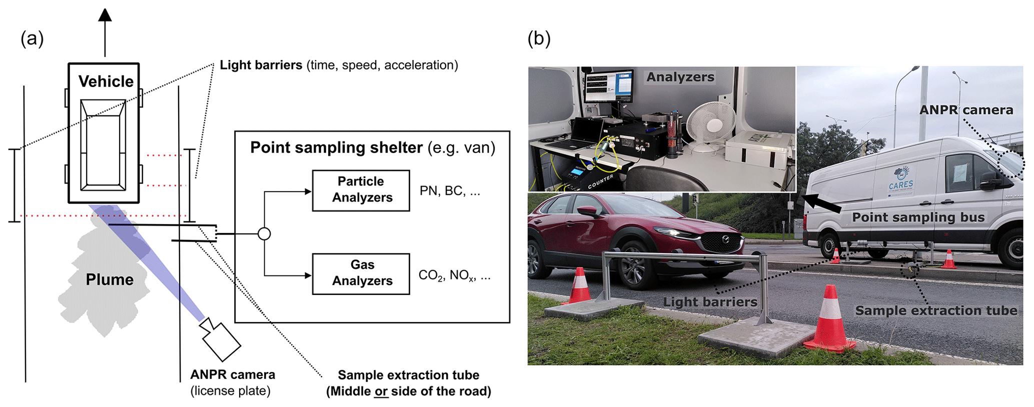
Figure 1Schematic (a) and photograph (b) of the proposed PS measurement setup highlighting the required equipment.
In this work, we present a comprehensive PS technique used for large-scale emission screening of individual vehicles, largely independent of the vehicle type. The PS setup measures different PM metrics as well as gaseous compounds and allows emission measurements to be carried out in dense traffic down to a distance of just a few seconds between the vehicles. The core of this work is a data analysis framework that is capable of processing data from thousands of vehicles. The main part of the data analysis is our peak detection algorithm (TUG-PDA)1, which separates emissions down to a spacing of a few seconds between the vehicles. We provide detailed insight into the PS methodology developed by discussing the dependencies and key factors, including instrument selection criteria, measurement site selection, sample extraction, vehicle dependencies and weather influences. We show the capability of the system by providing real-world BC, PN and NOx emission trends for passenger cars and HDVs up to the latest Euro emission standards. We use the term “pollutant” for all analytes measured except CO2. Important definitions for RES emission calculations are described in Appendix A.
2.1 Measurement setup
We propose a PS setup as illustrated in Fig. 1, which enables automated post-processing down to a small distance between the vehicles. The main components are described here.
Vehicle pass detection. The exact passing time of the vehicles is of great significance for automated post-processing. This is especially the case if several vehicles pass by the measurement location and they have only a small spacing between them. The exact passing time is required during data post-processing to resolve the different plumes correctly. Important variables related to the vehicle condition during the passing are the speed and acceleration. These are required to determine the vehicle specific power (VSP) (see Appendix A3). Emissions from passing vehicles strongly depend on the engine load conditions. Therefore, they must be treated accordingly (Bernard et al., 2018; Davison et al., 2020). For this purpose, we deployed custom-built light barriers to measure the passing time, speed and acceleration of the passing vehicles. Using light barriers restricts the measurement location to single-lane roads or roads with islands between the lanes. Alternatively, vehicle detection can be performed with radar, video or lidar systems.
License plate recognition. Vehicle technical data are required for several post-processing steps, which are described in more detail in the “Data analysis” section. Automated number plate recognition (ANPR) systems are commonly used for license plate detection. Depending on the system, additional attributes such as the vehicle pass time or acceleration can be measured. Attention must be paid to the ANPR camera performance, as several influencing factors can exist. License plates are often dirty (especially in winter) or the ANPR camera may not able to correctly detect the plates of all the passing vehicles, especially if they pass within short intervals. This impedes data post-processing and underlines the importance of accurate vehicle pass detection. In our setup, the ANPR camera is mounted in the front cabin of the measurement van (see Fig. 1), allowing the license plates to be detected about 2–3 s after the vehicle passes the light barriers. Based on our practical experience, we recommend determining the vehicle pass time separately from acquiring the license plate data.
Emission measurement. The emission measurement can be split into two main parts: first, the emissions are sampled and second, these are subsequently analyzed with the employed instrumentation. A schematic of the emission measurement setup used during one of the campaigns can be found in the Supplement.
-
Sampling. The importance of sample extraction is often underestimated. In PS, the sampling is usually performed with a simple tube which collects the diluted exhaust from the passing vehicles (Hak et al., 2009; Hallquist et al., 2013; Liu et al., 2019; Zhou et al., 2020). We sample either from the middle of the road or from the roadside depending on the circumstances (e.g., permissions, road conditions). When sampling from the center of the road, we cover the tube with a small cable duct that is taped to the road. The position of the sampling inlet strongly influences the strength (dilution) of the measured plume and even determines whether the plume can be captured at all. In general, the closer the sample inlet to the emission source (tailpipe), the smaller the dilution and the higher the capture rate. We found typical dilution factors between 100 and 500, which is in good agreement with the literature (Hak et al., 2009). In addition, the length of the sampling line must be considered in relation to the sample flow. The pressure drop should be minimal and the losses must be taken into account, especially when performing PM measurements (Kulkarni et al., 2011). Attention should also be paid to the material of the tubing. We use Tygon tubing for particle measurements because of the flexibility and low particle losses (Giechaskiel et al., 2012).
-
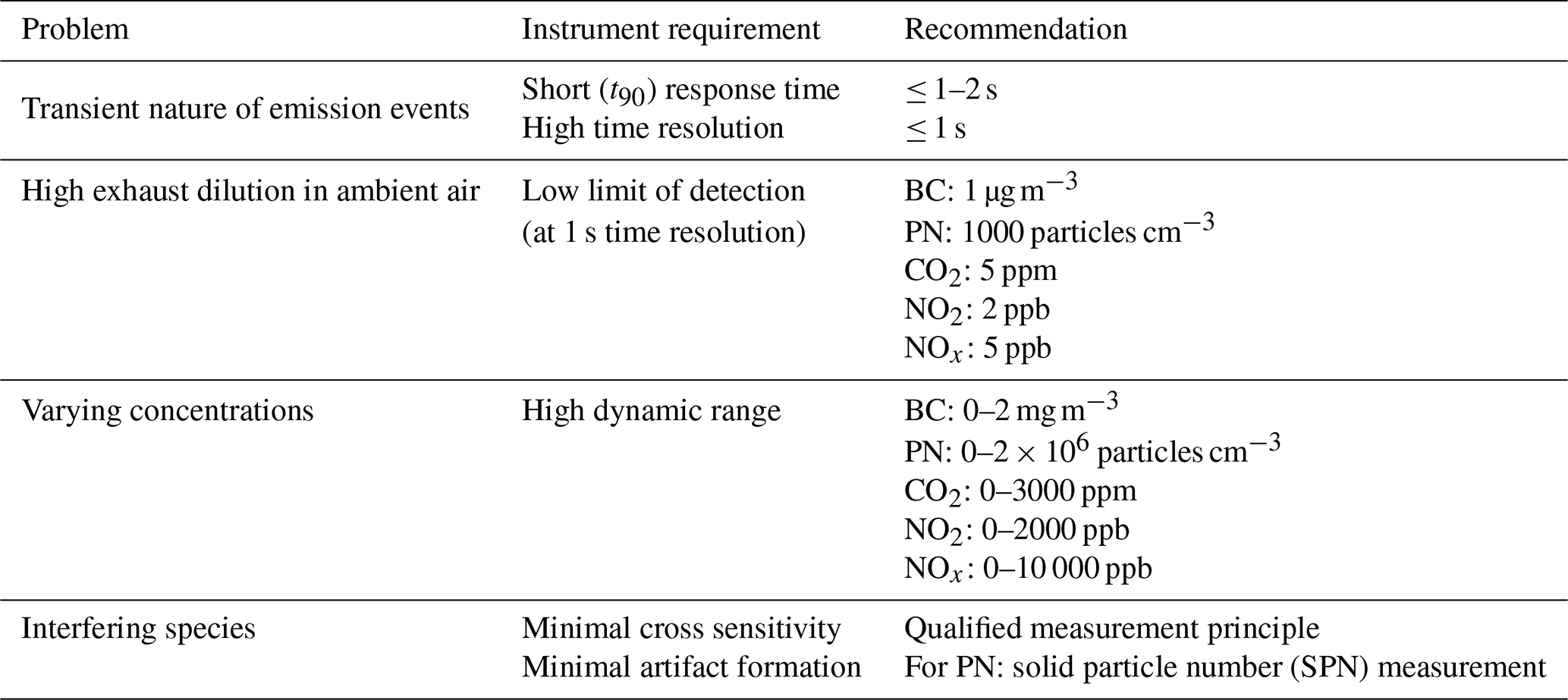
Instrumentation. Instrument characteristics have a great influence on the quality of the measured emission data. Sugrue et al. (2020) compared high- and low-cost BC and CO2 sensors for their application in PS. They found that low-cost CO2 sensors may be an adequate substitute for research-grade analyzers in contrast to low-cost BC instruments. In their conclusion, they also emphasized that sensors should be tested under field conditions. Hak et al. (2009) mentioned in their PS experiments that the small dynamic range of the condensation particle counter used constrained the PN measurements. Therefore, they used a dilution volume which extended the measured emission concentration peaks and the fall time of the signals to 5–15 s. The dilution and the relatively large response times of the particle instruments limited the operation to low-traffic situations. Based on the recommendations by Hak et al. (2009) and our own experience, we have defined the most important requirements for the instruments, which are listed in Table 1. These must be respected to avoid significant problems in PS. In addition, recommendations are given for the different requirements. The emission events associated with the passing vehicles are of a very transient nature. To capture these events, instruments must have a fast response time (t90 < 1–2 s) and a high time resolution (at least 1 s). In PS, the sampled emissions are highly diluted. Therefore, small concentrations must be resolved. To accurately measure the varying concentrations, the instruments must have a high dynamic range. The measured concentrations can be within a range of 4 orders of magnitude and depend on the vehicle type, engine state, sampling position and environmental conditions, as well as other factors. It is also important to ensure that the species of interest is measured with minimal cross-sensitivity to other compounds. Therefore, instruments with qualified measurement principles should be selected. Environmental conditions (e.g., temperature, relative humidity and background (BG) concentrations) differ depending on the measurement location, time and season of the year, and care should be taken to ensure that they do not affect the instruments. RES campaigns often last for long periods (several weeks or months). Therefore, instruments must be stable over the long term. Due to restrictions in the use of calibration sources such as gas bottles or particle sources, the instruments should feature stable calibration over periods of weeks even under harsh environments. Instruments which do not require in-field calibration are preferred. To perform measurements under all conditions, an instrument housing is required, which can be a small shelter or a measurement van.
Table 1Instrument requirements, problem statements and recommendations for PS emission measurements of selected particle metrics and gases.
Monitoring of environmental conditions. It is advantageous to make additional measurements of environmental conditions at the measurement location. Local monitoring of wind speed and direction provides information relevant for the sample extraction and can improve the post-processing. Measurements of precipitation, ambient temperature and relative humidity can also provide useful information and help to understand anomalies. We have used data from weather stations either in the area or preferably directly at the PS site.
2.2 Data analysis
The data analysis deals with the determination of representative EFs from the collected measurement data of the captured vehicles. The following aspects must be taken into account:
-
handling and harmonization of data (concentration time series) collected with various instruments;
-
consideration of measurement parameters such as sampling delay or instrument response times;
-
detection and separation of the plumes from the passing vehicles;
-
relation between vehicle pass (time), concentration time series and license plates;
-
dealing with changing environmental conditions (e.g., BG concentrations, other emission sources and weather conditions) that can affect the measurement.
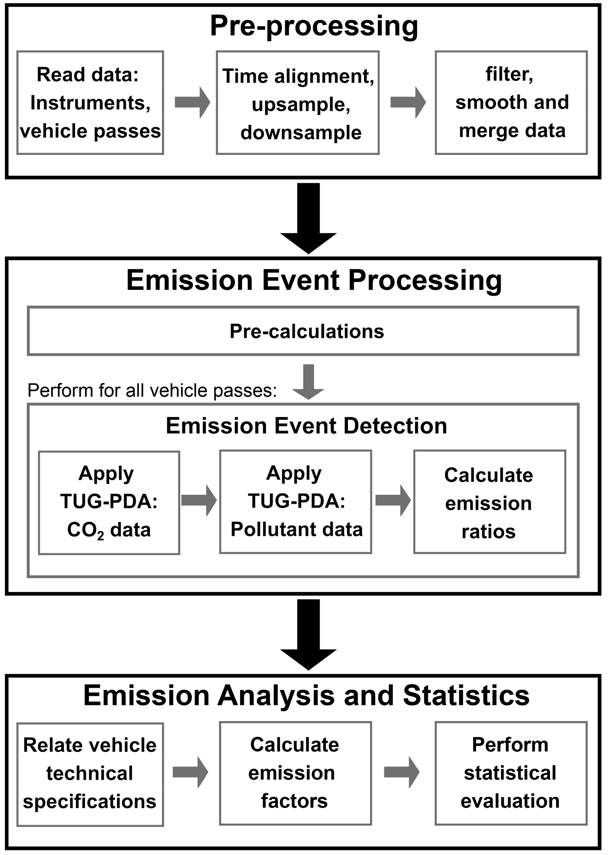
In order to deal with the requirements listed above, a comprehensive software framework has been developed. The procedure developed here is divided into three major processing steps, namely, the pre-processing, the emission event processing and the emission analysis and statistics. The pre-processing reads the raw time series files from various instruments and the recorded data from the light barriers (time, speed and acceleration) and prepares them for the next processing steps. These data are analyzed in the emission event processing part of the procedure. The EFs are then calculated in the emission analysis step, and statistical analyses are performed to subsequently evaluate the EFs. An overview of the data analysis procedure is presented in Fig. 2. The software framework is designed for modularity and extensibility. New instruments and measurement campaigns can be easily integrated into the framework by copying existing instruments or campaigns and adjusting the parameters. The software has not been developed for specific instruments, and in general any measurement device that provides continuous measurement data can be integrated. However, we strongly suggest considering the recommendations in Table 1 when selecting instruments in order to achieve the best possible results. The software framework is implemented in Python by using common libraries such as Pandas, NumPy, Matplotlib or SciPy. The basic framework of the software can be found at: https://gitlab.com/tug-ems/point-sampling.git (last access: 10 April 2024).
2.2.1 Pre-processing
Prior to the actual emission calculations, three main steps are taken to prepare the raw instrument data.
- 1.
Time series data from the different instruments are time-aligned based on manual pollution peaks (e.g., taken with a lighter) taken during the measurement campaign (time alignment to ± 1.0 s, see the Supplement).
- 2.
The time resolution of the CO2 and pollutant data is equated (default time resolution of 0.5 s), and the CO2 and pollutant datasets are combined into a composite dataset.
- 3.
The time series data are then smoothed with a rolling Gaussian filter (default window size-5 samples) to reduce the dependence on short variations and outliers. If instruments with large differences in response times (Δt > 2 s) are used, the response function of the instruments must be aligned.
2.2.2 Emission event processing
We have developed a dedicated algorithm, TUG-PDA, which separates the measured emissions and assigns them to the passing vehicles. The algorithm is fully configurable with various adjustable parameters defining thresholds or quality assurance (QA) measures. Figure 3 shows the main processing steps of the TUG-PDA algorithm, separated for CO2 on the left (Fig. 3a) and for pollutant emissions on the right (Fig. 3b). The TUG-PDA loops through all the vehicle pass data and is applied first to CO2 and afterwards to each pollutant (e.g., NOx, BC). The CO2 time series and the time series of the measured pollutants (e.g., BC, PN and NOx) are processed separately, since PM and gaseous emissions can occur at a different time. The main processing steps are the same, but several processing steps are only performed when processing CO2 emissions (plume strength) or when processing pollutant emissions (cross-checks with CO2). The processing steps are explained in the following paragraphs, including step numbers (and the letter “L” for low-emitter processing) that refer to Fig. 3 (TUG-PDA overview) and Fig. B1 in the Appendix B (TUG-PDA details).
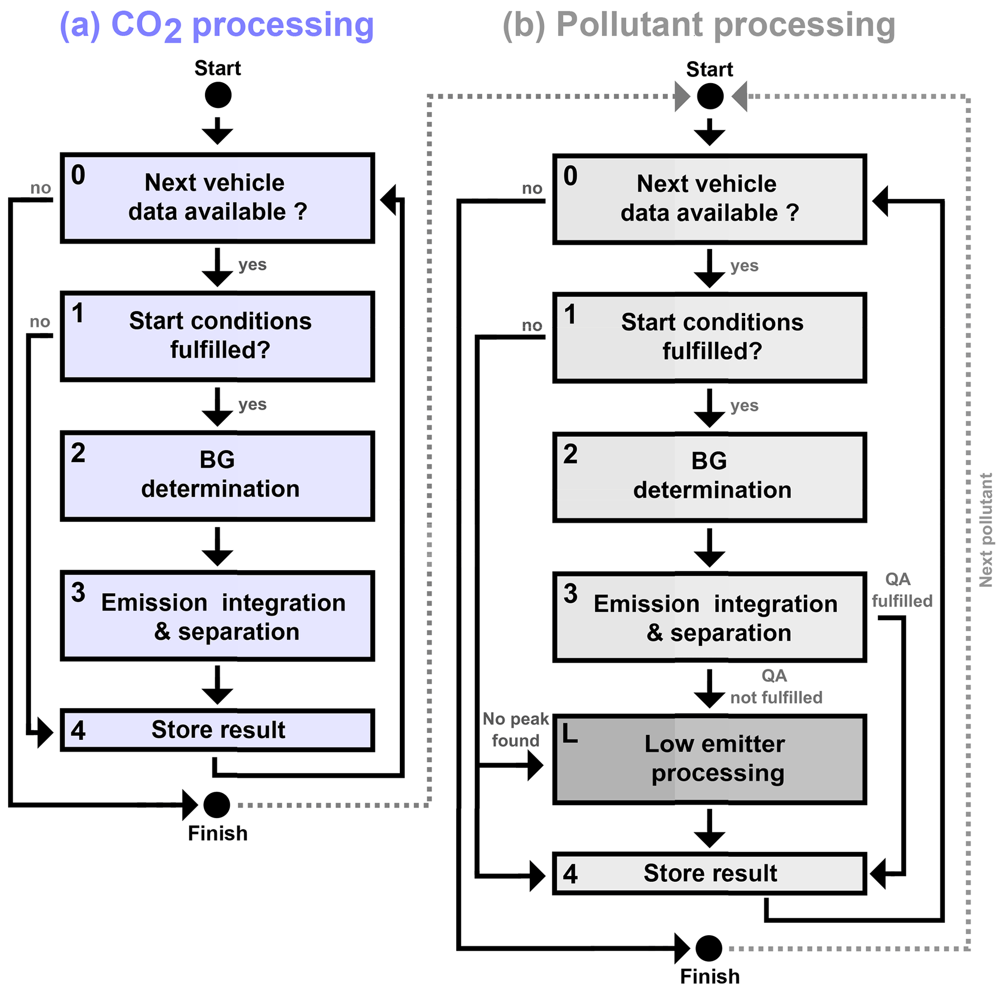
Figure 3Emission event processing – flowcharts of the peak detection algorithm (TUG-PDA). CO2 and pollutant (e.g., BC, PN, NOx) emissions are processed separately. The algorithm is applied first to CO2 (a) and then to the individual pollutant emissions (b). A detailed flowchart can be found in Appendix B (Fig. B1).
- 1.
Start conditions. The vehicle pass time is used as the starting point for the plume detection. Several QA measures (shaded boxes in Fig. B1) are implemented to prevent wrongly assigned emissions or inaccurate results. The following steps are performed, and the conditions must be met to continue processing the current vehicle.
- 1a.
Vehicle distance. First, when a new vehicle pass is fetched, it is checked whether the distance to the next vehicle pass is sufficient (≥ 3 s). If this is not the case, the processing of the current vehicle is stopped and the algorithm proceeds to the next vehicle. With a spacing of less than 3 s, there is a large uncertainty that emissions will be attributed to the wrong vehicle due to differences in the sampling delay between vehicles.
- 1b
CO2 emission valid. When processing pollutant emissions, the processing of the current vehicle is skipped if no valid CO2 plume was detected during CO2 processing.
- 1c.
Search for emission gradient (peak). The TUG-PDA searches (default window: from −1 to 6 s) for a sequence of data points with positive concentration gradients above a defined threshold (see Table 2) of the processed analyte around the vehicle pass time (illustrated in Fig. 4). There must be either at least two data points of the analyte with a gradient above the threshold or one data point with a very large gradient (> 10 times the threshold). The time of the first rising gradient is used as the starting point for the plume integration.
- 1d.
Separability. The detected gradient (plume) must not be from a previous vehicle. The processing is skipped if either
- -
a rising gradient (start condition) from the previous vehicle is found within a pre-defined time frame (default: 3 s before the vehicle pass of the current vehicle) and the plume directly interferes with the current vehicle or
- -
a significantly higher pollutant concentration was measured in the last period (default: 25 s) than for the current vehicle and the current vehicle is likely to be affected by this emission, which is the case when the emission of the previous vehicle was much higher than the peak of the current vehicle and the BG concentration before the current vehicle is still significantly higher than the BG without vehicles.
- -
- 1e.
Pollutant vs. CO2. The pollutant peak must start within a pre-defined window compared to the CO2 peak (default window: −1 to 3 s).
- 1a.
Table 2Default gradient thresholds defined in the TUG-PDA for the peak search.
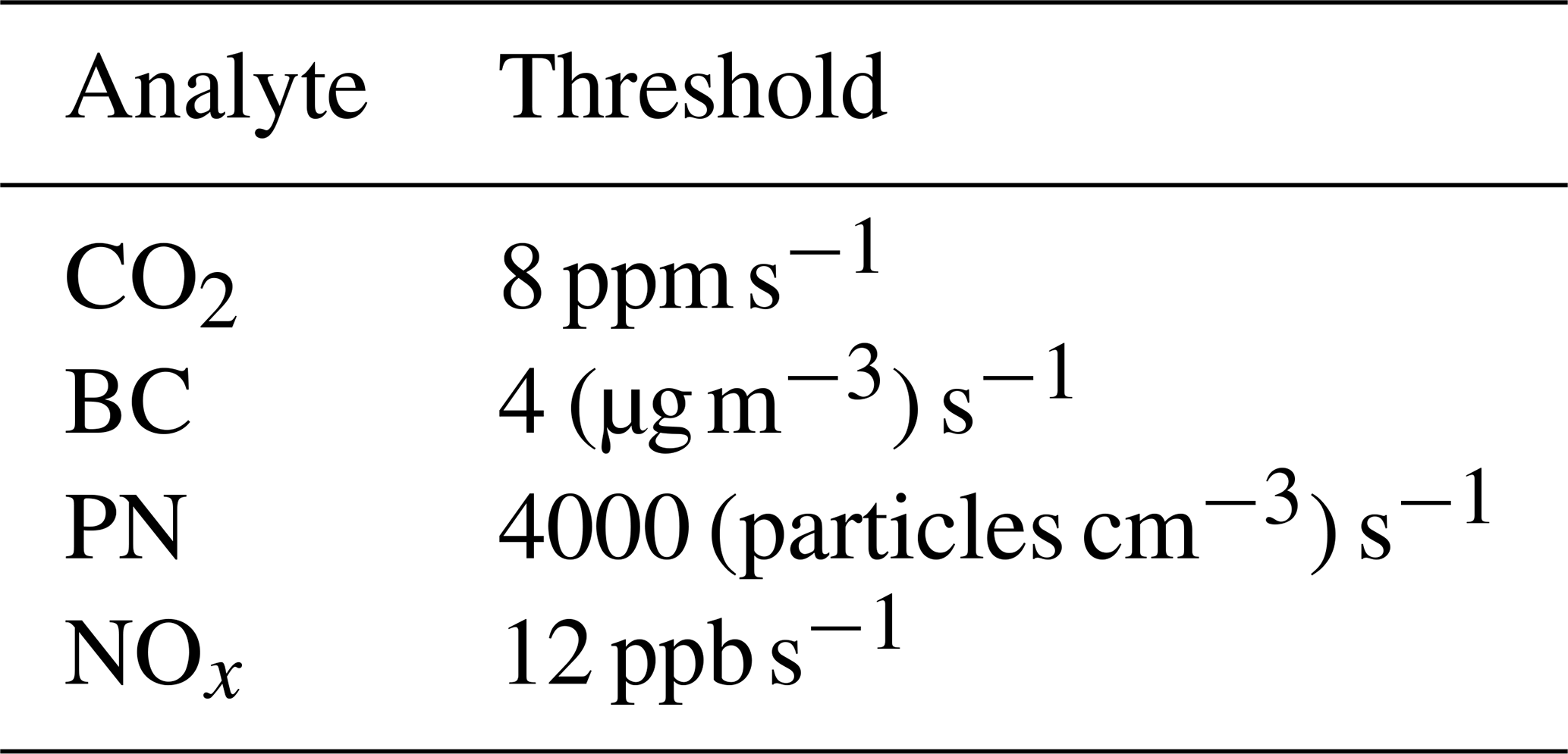
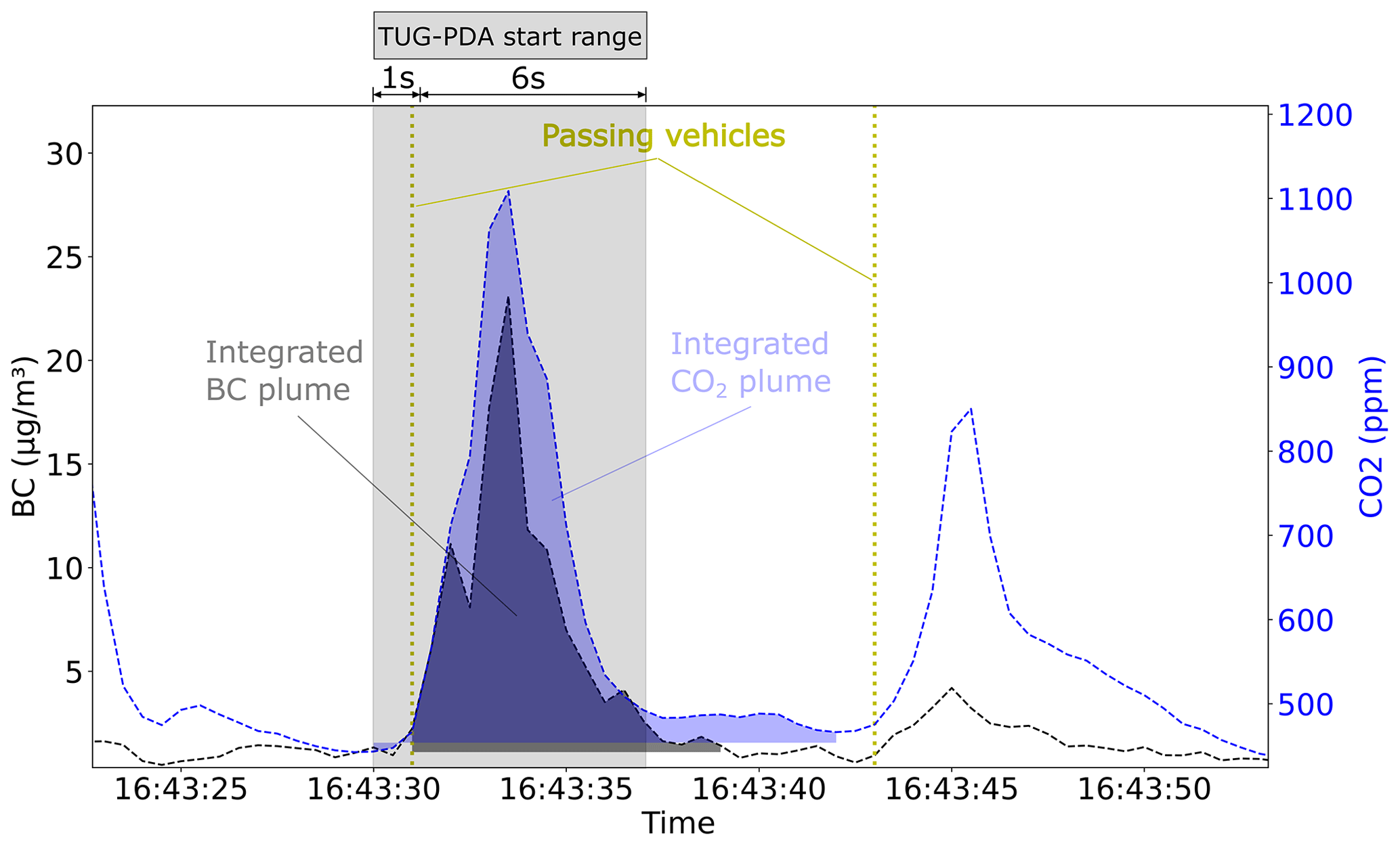
Figure 4Time series example of sampled PS data (BC, CO2) from two vehicle passes. The integrated areas of the CO2 and BC emission concentrations are highlighted for the first passing vehicle using the TUG-PDA as described in Sect. 2.2.2. The start time range of the algorithm is indicated for the first vehicle pass.
- 2.
BG determination. Before integrating the peak, the BG concentration is determined. We divide the BG determination into the following two cases:
- -
No interference. If there is no interference from a previous vehicle, this case is used. We found that the minimum of the running mean concentration just before the vehicle pass was the best fit as it represents the actual condition. In this study we used a window of 4 s (eight samples) before the integration start time. Similar approaches have been used in the literature to determine BG concentrations (Ban-Weiss et al., 2008; Wang et al., 2015).
- -
Interference. The plumes overlap when vehicles pass the measurement point within a short period. In this case, the mean value is taken between the median concentration directly before the starting point of the integration (default window size: 3 s) and a general BG value taken within the last few minutes that is not influenced by vehicles. Here we search for the last time frame in which no vehicle plume was detected. If no such window (default length: 8 s) is found in the last 10 min, a statistically determined BG value is calculated by removing emissions above the 75th percentile of the dataset used. A moving average filter (default window size: 30 s) is applied to the resulting dataset and the minimum value is used as BG. Examples of BG-subtracted emissions from overlapping plumes are shown in Fig. 5.
- -
- 3.
Emission integration and separation. After determining the BG, the concentration of the exhaust plume is integrated until one of the defined stop conditions is reached (see Fig. B1):
- -
Stop 1. The maximum allowed duration (default length: 25 s) of the emission event is exceeded.
- -
Stop 2. The concentration falls below the BG concentration.
- -
Stop 3. Another vehicle pass is observed and the concentration gradient increases.
- -
Stop 4 (pollutant only). The pollutant integration exceeds the stop time of the CO2 event by a defined value (default: 3 s).
- -
Stop 5 (pollutant only). The integration interval of the pollutant emission event (duration of the integrated areas) exceeds the integration interval of the CO2 emission event by a defined value (default: 1 s).
In addition to the QA measures applied during the start conditions, the following tests are performed after the integration to verify whether the emission is considered valid:
- 3a.
Duration. The integration interval must exceed a minimum value (default: 3 s).
- 3b.
Plume strength (CO2 only). The integrated CO2 area must be greater than a defined minimum (default: 80 ppm s).
- 3c.
Pollutant vs. CO2. The integration interval of the CO2 emission event including a predefined factor (default: tmax diff = 0.6) must not be greater than the integration interval of the pollutant emission event.
- 3d.
Pollutant vs. CO2. The CO2 and pollutant integration intervals must overlap to a certain extent (default: by at least 50 %).
- -
- L.
Low-emitter processing. When processing the pollutant data, a special case is implemented in order to consider low emitters (Fig. 3, highlighted in dark gray). This is the case if no emission gradient (peak) is found, if the duration of the emission event is below the lower limit of the integration interval or if the integration interval of CO2 is too long compared to the integration interval of the pollutant. If one of the three conditions is not met, then the pollutant concentration is integrated over the same time period as the captured CO2 event associated with the passing vehicle. Similar to the general procedure, the BG determination is separated into the two cases described (without/with interference) and the integration is stopped if another vehicle pass is observed and the measured concentration increases.
- 4.
Store results. The emission event is considered valid (highlighted in green in Fig. 3) if the start and post-integration QA conditions are met. If these conditions are not met, the emission event is invalid. The TUG-PDA continues processing the next vehicle pass.
Once the TUG-PDA has finished processing all the vehicle passes, the emission ratios (ER) of each vehicle pass (see Sect. A1 in the Appendix) are calculated.
Alternative methodologies exist for emission processing in PS. The captured CO2 and pollutant emissions are commonly integrated over the same time frame (Ban-Weiss et al., 2009; Ježek et al., 2015; Liu et al., 2019; Zhou et al., 2020). Automated PS emission processing and peak detection algorithms can also be found in previous studies. Wang et al. (2015) presented a plume identification algorithm that takes different approaches in the case of plume separation (minimum plume length of 10 s) or low-emitter detection. An open-source mobile air quality dashboard, including a real-time peak detection algorithm, was published by Kelly et al. (2023). Another new approach proposed by Farren et al. (2023) is the so-called rolling regression method. This algorithm simplifies data processing by calculating the ERs for three consecutive data samples, which makes the BG determination redundant. This is a particularly promising approach for short emission events of high emitters. One challenging aspect of this approach is the determination of low emissions from the latest emission standards. Another aspect is that the instrument responses for the CO2 and measured pollutants must be perfectly matched when taking this approach. The applicability of this approach to evaluating PM pollutants still needs to be studied due to the disparity between gaseous and PM emissions.
2.2.3 Emission analysis and statistics
Once the ERs of passing vehicles have been determined, the measurement results are combined with the vehicle's technical data. Several details from the vehicle technical data are required during the emission analysis to calculate EFs and to perform further statistical analysis. Necessary fields for our post-processing are as follows:
-
The fuel type (e.g., gasoline, diesel) is used to calculate fuel-based EFs.
-
The CO2 emissions measured during the type-approval process of the vehicle model are required to calculate the distance-related EFs.
-
The European emission standard class is used to classify vehicles according to their emission limits.
-
The vehicle category is used to perform detailed evaluations for specific vehicle types.
With the help of our local partners, we obtained the necessary technical data from the government authorities. The captured license plates are pseudo-anonymized to respect privacy rules.
As part of our data post-processing procedure, the vehicle technical data as requested from the authorities and detected by the ANPR camera must be related to the ERs. These are then assigned to the passing time as gathered with the light barriers. We use the speed and acceleration information of the passing vehicles to match the passing time with the detected license plate. This generally sounds like a simple task. However, not all license plates are correctly detected by the ANPR camera for various reasons (e.g., dirt, poor light conditions or too little distance between the vehicles). This makes the task of correctly matching the data from the ANPR camera and light barriers challenging, and specially for vehicles that follow each other closely.
2.3 Capture rate
In RES, the proportion of valid measurement records is a significant indicator. We call this indicator the “capture rate” (CR), which is the ratio between the number of vehicle passes for which valid EFs can be calculated and all vehicle passes (Eq. 1).
What is considered as a valid measurement is always subjective. We consider the calculated emissions to be valid if the plume from the passing vehicle was properly captured and an EF can be calculated. This is the case if the following conditions are considered to be true:
-
The integrated CO2 plume is greater than a specified threshold. In this study, 80 ppm s was used.
-
The emissions of the passing vehicle can be separated from those of other vehicles. This is not the case if the plumes cannot be separated or if the emissions cannot be unambiguously assigned to one vehicle (see Fig. B1).
3.1 TUG-PDA emission separation capabilities
The TUG-PDA resolves emissions down to a small distance (default: 3 s) between vehicles if the time between the vehicles is large enough (greater than 3 s) and if a dedicated CO2 peak from the vehicle is observed. Several tests are implemented to determine whether the emissions really come from the current vehicle or are caused by interference from previous vehicles or another source. If other influences are observed, the distance between the vehicles is too small or overlapping plumes cannot be separated, the measurement is invalid and the emissions for the vehicle cannot be determined. Plume separation can be tuned using several parameters such as gradient thresholds (Table 2), the minimum time allowed between vehicles or the minimum number of samples required as used in the software. This can be very useful for instruments with different response times and for locations with dense traffic to obtain a sufficient number of measurements. Restricting measuring to low-traffic areas would severely limit the application.
Figure 5 shows two PS time series examples that demonstrate the capabilities and the limitations of the TUG-PDA for plume separation from passing vehicles. The BC and CO2 emissions assigned to the passing vehicles are highlighted in black and blue, respectively. In both examples, the BG concentrations are subtracted from the integrated areas. In the data shown in Fig. 5a, the TUG-PDA is able to separate emissions for three (V1, V3, V4) out of four vehicles. CO2 and BC peaks are evident for all four passing vehicles, but to varying degrees. For vehicles V1 and V3 the algorithm stops integrating the emissions because another vehicle (V2 or V4) is passing and the concentrations are rising. For vehicle V4, the integration is stopped because the BG value is undercut. The plume detected from vehicle V2 is invalid because the CO2 gradient is not above the threshold and the integrated area is below the minimum value (80 ppm s). The algorithm can be easily tuned to detect emissions from vehicle V2, but as plume strength decreases, inaccuracies increase. This is due to the increasing dependence on the BG determination and is even more pronounced when the plumes overlap. Figure 5b shows a data example where the emissions of most passing vehicles cannot be resolved properly due to high traffic density. The emissions of vehicles V1 and V2 can be resolved, as the distance between the vehicles is large enough (≥ 3 s) and two distinct CO2 peaks are detected. Both vehicles can be considered low BC emitters, as no BC peaks were measured. No EFs can be determined for vehicles V4, V5, V8, V9 and V10 because the distance between the vehicles is too small and no distinct CO2 peaks can be assigned to them. Vehicles V3, V6 and V7 do not show clear CO2 peaks, either because they are too weak or because they are superimposed by the emissions of a preceding vehicle.
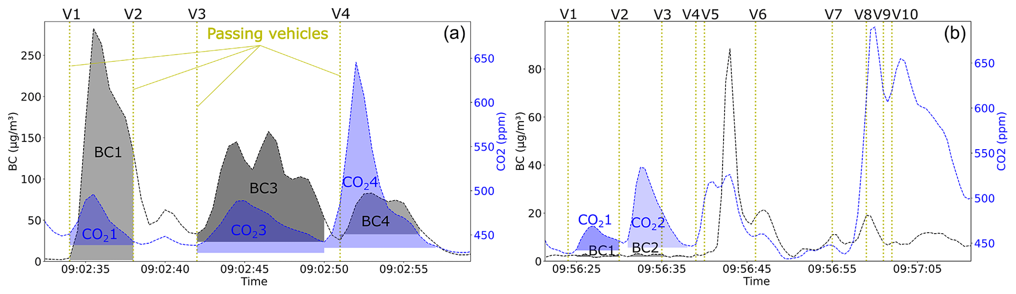
Figure 5Two PS time series examples (BC, CO2) from captured plumes. The vertical dashed yellow lines mark the point at which the vehicles passed the PS spot. (a) Emissions can be separated for three (V1, V3, V4) of the four vehicles. The assigned emissions are highlighted in different colors (BC1–BC4 and CO21–4). (b) For most vehicle passes, the emissions of individual vehicle passes are not separable. Ten vehicle passes are shown, of which emissions are determined for two (BC1,2 and CO21,2).
In the current implementation of the TUG-PDA, the BG determination for overlapping plumes is done by calculating an average value between the median concentration directly between the overlapping plumes and a common BG when no vehicle is passing. This is a simple estimation and entails deviations from the actual situation. This can be seen, for example, in Fig. 5a for vehicle V4. The BC background is overestimated. This results in a too small integrated area (BC4) and thus in underestimated emissions. This can also be seen to a smaller extent for vehicle V3, where both CO2 (CO23) and BC (BC3) backgrounds are underestimated, leading to an overestimation of both areas.
It is important to know how accurate the determined EFs are due to the assumptions made in the calculations for overlapping plumes and the complexity of resolving superimposed emissions. We therefore assessed the impact of interference from other vehicles and pollution sources on the resulting EFs. The TUG-PDA distinguishes between the following three cases of interference:
-
Overlap. The plume from the current vehicle overlaps with the plume of a previous vehicle. The two plumes must be separated.
-
Cut-off. The plume from the current vehicle interferes with the next vehicle. The emission integration stops for the current vehicle, and the entire plume has not been captured.
-
Overlap + cut-off. The above two cases are applicable. The plume from the current vehicle is influenced by the plume from the previous vehicle and the exhaust plume from the next vehicle.
These cases are marked in the algorithm and can be used for further analysis. This marking is done individually for the different emission signals (e.g., CO2, BC, NOx), as they are processed separately.
As an example, we investigated the influence of interfering plumes on the determined BC emissions of petrol-powered passenger cars. Only overlapping CO2 signals are taken into account and no superposition of BC emissions. The inclusion of BC interferences distorts the results, as these consist mainly of high emitters (see Fig. C1). The emission distributions shown (Fig. 6) are separated into a combined dataset (with and without interference), measured interference-free emissions and the three cases in which the TUG-PDA categorizes interference. We did not find a strong influence of plume interference on the results. The determined EFs are statistically comparable between the different datasets with and without interference from other vehicles. The largest deviation was found for plumes that were cut-off. The median EFs were 19 % lower than in cases without interference. The sample size shows that the majority of the emissions determined were influenced by an interference. When only plumes without interference were considered, the number of measurements would be greatly reduced. We also looked at how accurate the EF can be calculated using only a fraction of the plume. Therefore, we selected only plumes without interference from other vehicles, and we calculated EFs using the TUG-PDA when the algorithm used only a fraction of the plume in the interval between 3 and 23 s. Similar to the investigation shown in Fig. 6, we found that when only a fraction of the plume is used the EFs are underestimated. The median underestimation for an early cut-off at 3 s is 27 %. The deviation decreases with the increasing fraction of the plume (see Fig. C2).
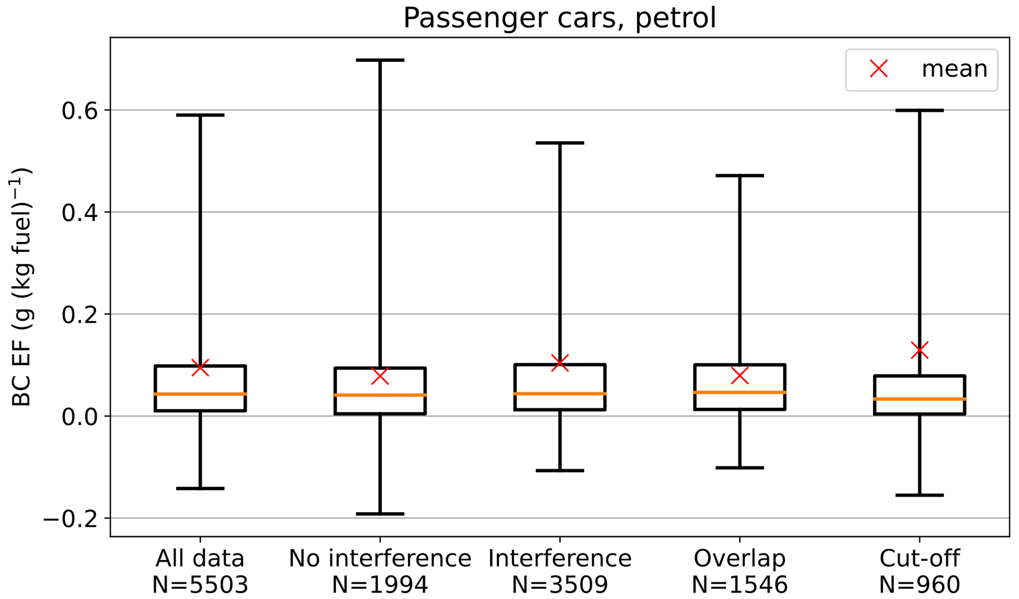
Figure 6Influence of interference from other vehicles or pollution sources on the BC emission distributions determined with the TUG-PDA. Measured EFs of petrol-powered passenger cars are used for comparison. Interference data include both overlapping plumes and plume cut-offs (interference = overlap and/or cut-off). The whiskers represent the 2.5 and the 97.5 percentiles.
3.2 Factors influencing point sampling measurements
In this section, the most important factors influencing PS measurements are discussed, and the resulting impacts are shown on the basis of around 100 000 vehicle emission records gathered during four measurement campaigns. The measurement campaigns were conducted in the Netherlands, Italy, Poland and Czechia as part of the EU H2020 City Air Remote Emission Sensing (CARES) project. The results include data from nine monitoring sites, with data from the specially developed Black Carbon Tracker (BCT) being used to assess the various factors. The BCT measures BC with a photoacoustic-based sensor cell and CO2 with a non-dispersive infrared (NDIR) sensor integrated into one device. The device was developed based on the recommendations listed in Table 1 as part of the CARES project (Knoll et al., 2021). The impact of misaligned measurement data on the resulting ERs is discussed in the Supplement.
3.2.1 Instrument characteristics
For our study we selected two instruments, our custom-designed BCT and the Aethalometer AE33 (Magee Scientific), for their applicability in determining BC emissions using the developed TUG-PDA. The Aethalometer AE33 is widely used in environmental science for BC measurements and source appointment and is commonly used in PS studies to quantify BC emissions (Ježek et al., 2015; Preble et al., 2018; Zhou et al., 2020; Sugrue et al., 2020). We characterized the BCT and the AE33 in the laboratory for properties relevant for PS (see Table 1). A miniCAST soot generator (Jing Ltd., Model 6204 Type B) was used as the particle source. The instruments were measured in parallel downstream of a catalytic stripper which removed volatile compounds (Knoll et al., 2021). The measurements showed a very good correlation (R2 = 0.99) between the Aethalometer and the BCT. Comparable limits of detection (1 s, 3σ) were determined for both instruments, with values of 1.01 µg m−3 for the Aethalometer and 1.12 µg m−3 for the BCT. The limit of detection of the instruments defines the extent to which emissions can be resolved. This is particularly important for accurately quantifying emissions from vehicles that meet the latest emission standards. The t90 response times of the two instruments were measured in the laboratory: 0.9 s for the BCT and 7 s for the Aethalometer. A small response time enables the separation of highly transient emission events. This determines how close vehicles can drive to each other in order to be able to resolve the emissions. Figure 7 shows two emission time series of the two instruments during one of the measurement campaigns. Two vehicles pass by the PS spot during the time frame shown with an interval of 6 s. The BCT responds quickly to the BC emissions captured from the first passing vehicle (V1). A distinct peak is noted where the measured concentration is again below 10 % of the peak concentration of the first vehicle when the second vehicle (V2) passed by. The emissions captured for the two vehicles overlap, but they can be separated using the BCT. In contrast, the AE33 response time is much slower, and the maximum concentration is reached after the second vehicle (V2) has passed by. In this case it is not possible to separate the BC emissions of the two vehicles using the AE33. This example illustrates the importance of choosing instruments with a fast response time when measuring in dense traffic. Individual characteristics (see Table 1), such as the response time, that do not meet the requirements severely limit the application. However, the Aethalometer can also be used for PS, as has already been demonstrated in several studies. The traffic density must be low enough (distance between vehicles greater than 7–10 s) or only certain types of vehicles (e.g., HDVs with vertical exhaust pipes) are measured, which naturally entail a greater distance between exhaust plumes.
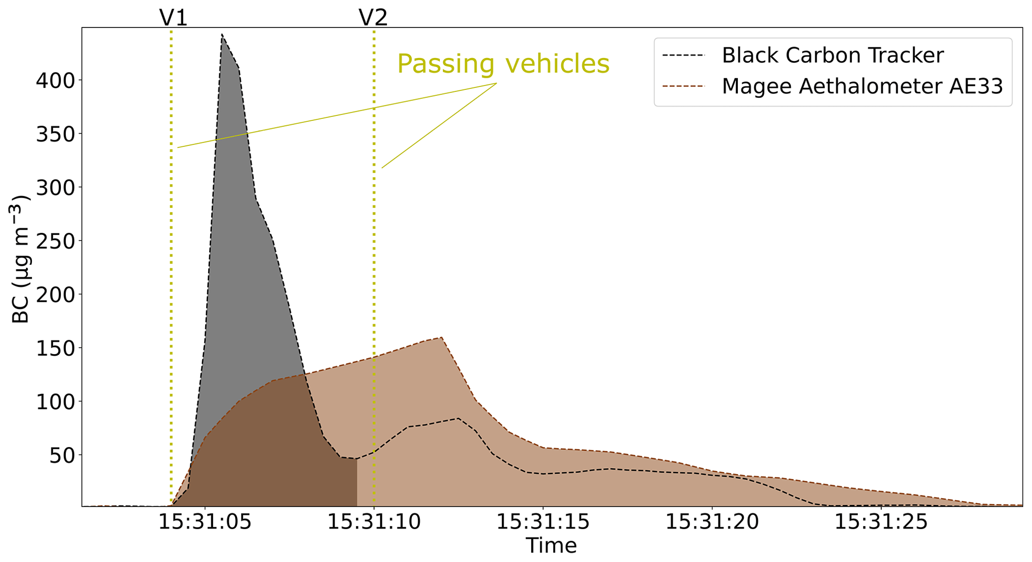
Figure 7Emission concentration time series example of two instruments with different response times. Areas shaded in gray (Black Carbon Tracker) and brown (Magee Aethalometer AE33) show the integrated areas of the BC emissions from the first passing vehicle as determined with the TUG-PDA.
3.2.2 Measurement location and sampling position
Special care must be taken when selecting suitable measurement locations. Besides the legal regulations (e.g., for the placement of equipment), the following aspects influence the selection:
-
road properties (single or multi-lane, lane width, road gradient)
-
traffic conditions (traffic flow, distance between passing vehicles, number and type of vehicles) and vehicle operating conditions (VSP, see Appendix A3)
-
influence of environmental and background conditions (see the Supplement)
-
cross-interference from other pollution sources.
In the following evaluations (e.g., Figs. 8 and 9), we assess the influence of the aforementioned aspects on PS measurements. The results from the different measurement locations are labeled with numbers. Different sampling positions or traffic situations were evaluated on individual locations. These are labeled with x.x (e.g., 1.1). This should facilitate the interpretation of the results and the comparison between the different impact factors, as they were not determined independently.
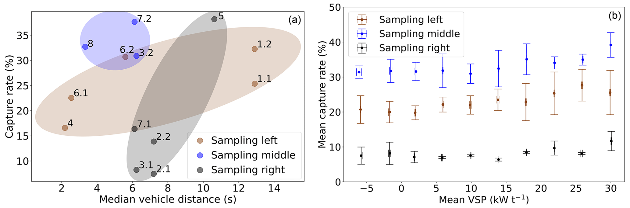
Figure 8Evaluation of two traffic-related impact factors and their influence on the capture rate. (a) The capture rate is shown as a function of the median vehicle distance at different measurement locations (indicated by numbers as in Fig. 9). (b) The VSP values calculated are clustered and shown separately for the different sampling positions.
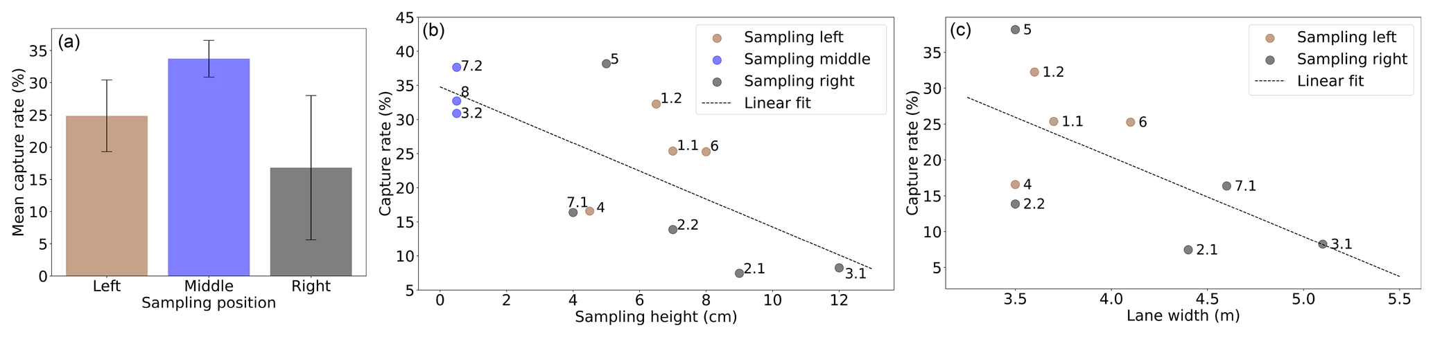
Figure 9Three plots show the influence of the sampling position and road width on the capture rate. (a) Mean capture rate at the three sampling positions, combined from all measurement sites. (b) Capture rate as a function of the height of the sampling inlet. The measurements were performed at different measurement locations, which are indicated by the numbers. (c) Capture rate as a function of the lane width for roadside measurements.
One selection criterion of PS campaigns is often the number of vehicles per site and day. Conducting campaigns on highly frequented roads guarantees a high number of vehicle passes. This is beneficial to a certain extent, as it allows for the collection of a large number of emission records. If the traffic density is too high for PS, the emissions from the individual passing vehicles cannot be properly resolved because they are superimposed (e.g., Fig. 5b). Not only the traffic density, but also the general traffic flow must be considered. Measurements are often performed after a crossroad or traffic light. Such conditions can lead to a high number of vehicles passing within a short period and a short distance from each other. This prevents emissions from being properly resolved. Therefore, we evaluated the CR as a function of the median vehicle distance at different measurement locations. The CR generally increases with median vehicle distances at the measurement locations (Fig. 8a). It is noticeable that even in relatively dense traffic (median vehicle distances 3.3–6.2 s), a high CR (31 %–38 %) can be achieved if the sampling is done from the middle of the road.
In order to select the measurement site, the road itself and the topography must be evaluated. We examined the influence of the VSP on the CR for the three sampling positions (left, middle, right). For this investigation, only speed, acceleration and the road gradient were used to calculate the VSP (see Appendix A3). The VSP values determined for the different measurement locations are clustered and averaged. We observed only a small impact of the VSP on the CR (Fig. 8b). The CR increases slightly with increasing VSP regardless of the sampling position. A certain engine load (e.g., VSP > −5 kW t−1 according to Bernard et al., 2018) is required for the measured vehicles, which can be accomplished in locations with a positive road gradient or at locations where vehicles accelerate (e.g., road crossings, slip roads). Roads with declining gradients should generally not be chosen due to a lack of engine load. The road type must be considered in terms of space for the measurement setup and cross-interference from other vehicles. In general, single-lane roads are preferred, as well as two-lane roads where the measured direction has a positive gradient. Vehicles driving in the opposite lane have a negative VSP and therefore only a small influence on the measurements.
The approach used to collect the exhaust has a major impact on the quality and strength of the signal. We found a direct relation between the CO2 signal strength (see the Supplement) and the CR (Fig. 9a). A higher CO2 signal generally leads to a higher CR. The highest CR can be achieved if the sample extraction is performed from the middle of the road. By using this central setup, a CO2 plume could be captured for an average of 34 % of the vehicles. Sampling from the left roadside delivers on average a CR of 25 % as compared to 17 % if the sample is extracted from the right side. In most regions in Europe, sampling from the left is favored over the right side. Vehicles from manufacturers in Europe (e.g., VW, BMW, Mercedes, Fiat) usually have the tailpipe on the left-hand side, unlike manufacturers in Asia or the United States (e.g., Toyota, Kia). At two measurement locations (3 and 7), the sampling was conducted from both the roadside and the center of the road. When sampling from the middle of the road (Figs. 9b and 8a), 2–3 times higher CRs were obtained. Measurements from the center of the road enable sample extraction in the closest proximity of the source and are therefore less influenced by traffic (Fig. 8a), wind or tailpipe position. We found no significant influence on the driving behavior when the sampling was done from the center of the road through the covered tube. In addition to the influence of the sampling side, the sampling height also has a major impact on the sample extraction. Higher CRs and stronger CO2 signals are achieved at lower sampling inlet heights for most vehicles in Europe. L-type vehicles (e.g., motorcycles) are an exception, with tailpipes pointing straight or even upwards. The width of the road has a non-negligible impact on measurements from the roadside (Fig. 9b). At two locations (1, 2), the sampling was conducted at two positions (1.1, 1.2 and 2.1, 2.2) at the same roadside with differences in road width and sampling height. For both, it can be seen that a smaller road width and a lower sampling height lead to a higher CR. Measurement locations where the sampling was done from the right side (2, 3, 5, 7) generally have a rather low CR. An exception is location 5, where the highest CR of all measurement sites was achieved. Location 5 stands out with good characteristics of all influencing factors such as a small lane width (3.5 m), a low sampling height (5 cm) and a high median vehicle distance of 10.6 s (∼ 2500 vehicles per day). The highest absolute number of valid measurements per hour was achieved at location 8 with 103 valid ERs per hour.
3.2.3 Weather conditions
Harsh weather conditions can have a substantial impact on RES measurements. For both PS and RES, the literature lacks detailed assessments that examine the effects of environmental conditions. Of particular interest are the dependencies related to precipitation and wind conditions. During the measurement campaigns, a weather station was located either directly next to the PS site or in the vicinity. The weather data used were available on at least an hourly basis. To allow an unbiased comparison to be made, only datasets were used where the compared meteorological conditions were present during the measurement campaigns.
Rain. We found that the PS measurements were not significantly influenced by rain. CRs are comparable during rainy (29.3 %) and dry (29.8 %) conditions (Fig. 10a). Similar values were also determined for the average CO2 plume of the passing vehicles. During dry periods, an average CO2 plume of 525 ppm s was measured as compared to 536 ppm s under wet conditions. We were particularly interested in discovering whether these conditions impacted PM emissions. For this purpose, we performed a Monte Carlo simulation by drawing 100 samples of the measured ERs of the passing vehicles from the different measurement sites 1000 times. We calculated the mean ERs from the 100 samples, and the distribution of the mean values is shown in Fig. 10b. Statistically, no significant difference was observed between the ERs calculated in dry and rainy conditions, with median values of 110 and 134 mg (kg CO2)−1, respectively. The slight differences may result, for example, from different driving behavior in wet conditions.
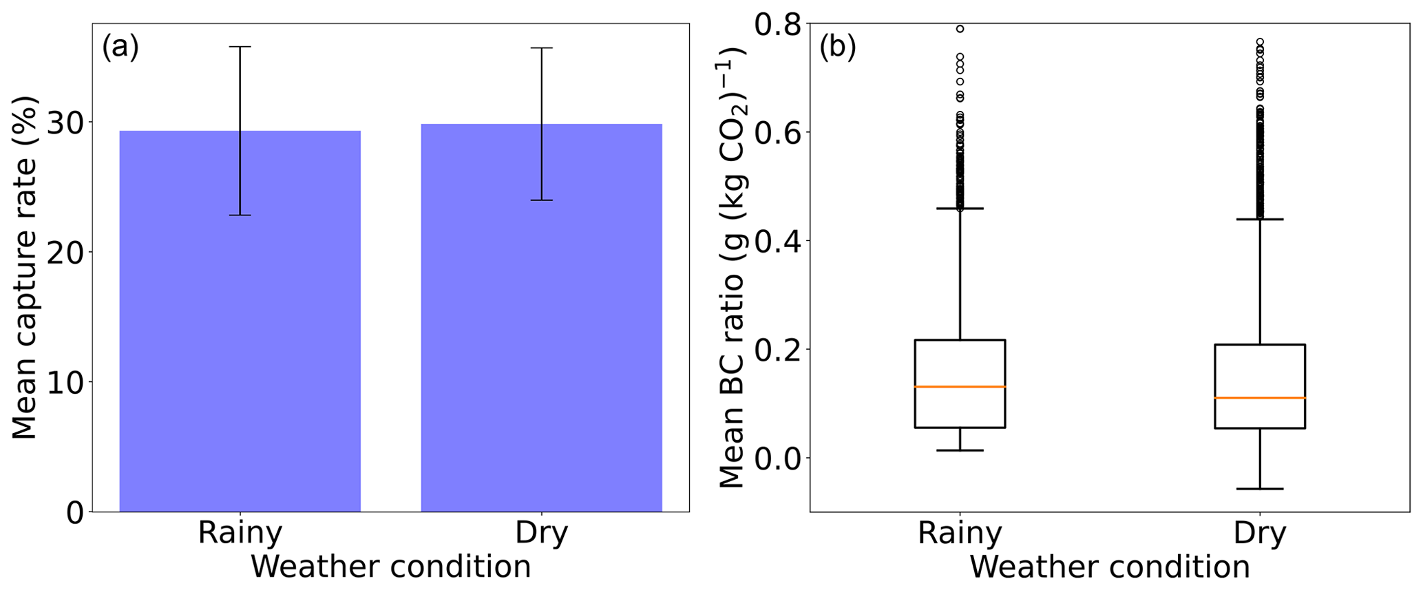
Figure 10Effect of precipitation on PS measurements. Measurements are compared for rainy (> 0.05 mm h−1) and dry weather conditions. Capture rates (a) and mean BC ratios (b) measured in both conditions are compared.
Wind. Wind direction and wind speed affect the dilution and transport of the plume. We assessed the effect of wind speed and wind direction on the measurements. The wind speed was segmented according to the Beaufort scale (Singleton, 2008). We found that with increasing wind speed the CR steadily decreases (Fig. 11a). A similar trend can be observed for the measured average CO2 plume of the passing vehicles. A higher CO2 signal (519 ppm s) was measured under calm conditions (< 20 km h−1) than under windier (21–39 km h−1) conditions (425 ppm s). A similar influence of wind speed on the CR was reported by Dallmann et al. (2011) in their top–down PS study for HDVs. They reported lower CRs in June (61 % unsuccessful plume captures) than in November (36 % unsuccessful plume captures), where average wind speeds were twice as high. In contrast to our results, they found that the dilution of the captured plumes was similar for both wind conditions.
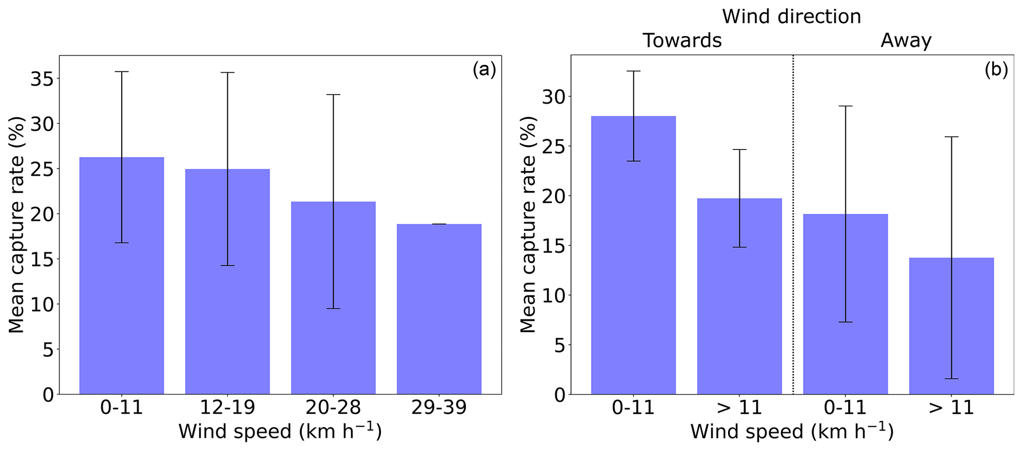
Figure 11Influence of different wind conditions on the capture rate. (a) Wind speed at urban measurement locations. (b) Wind speed and direction at a rural measurement site.
Not only the wind speed is relevant, but also the direction in which the wind blows the exhaust plume. We evaluated the impact of the wind direction on the PS measurements under calm (< 11 km h−1) and breezier (> 11 km h−1) conditions. For this purpose, we separated the wind directions into wind blowing the exhaust plume towards the measurement location and wind blowing it away from the sampling point. The wind directions are indicated in the Supplement. A significant influence was observed at a rural measurement location (Fig. 11b). The CR is higher under calm conditions and when winds are blowing towards the sampling position. We performed the same evaluation in urban environments. Here, we could not observe such a trend with similar CRs regardless of the wind direction (see the Supplement). We assume that this is mainly related to differences between the local wind conditions (local turbulence) directly at the PS spot and the wind measured at the weather station. Generally, wind conditions in street canyons are much calmer than those in open spaces, which is beneficial for PS applications.
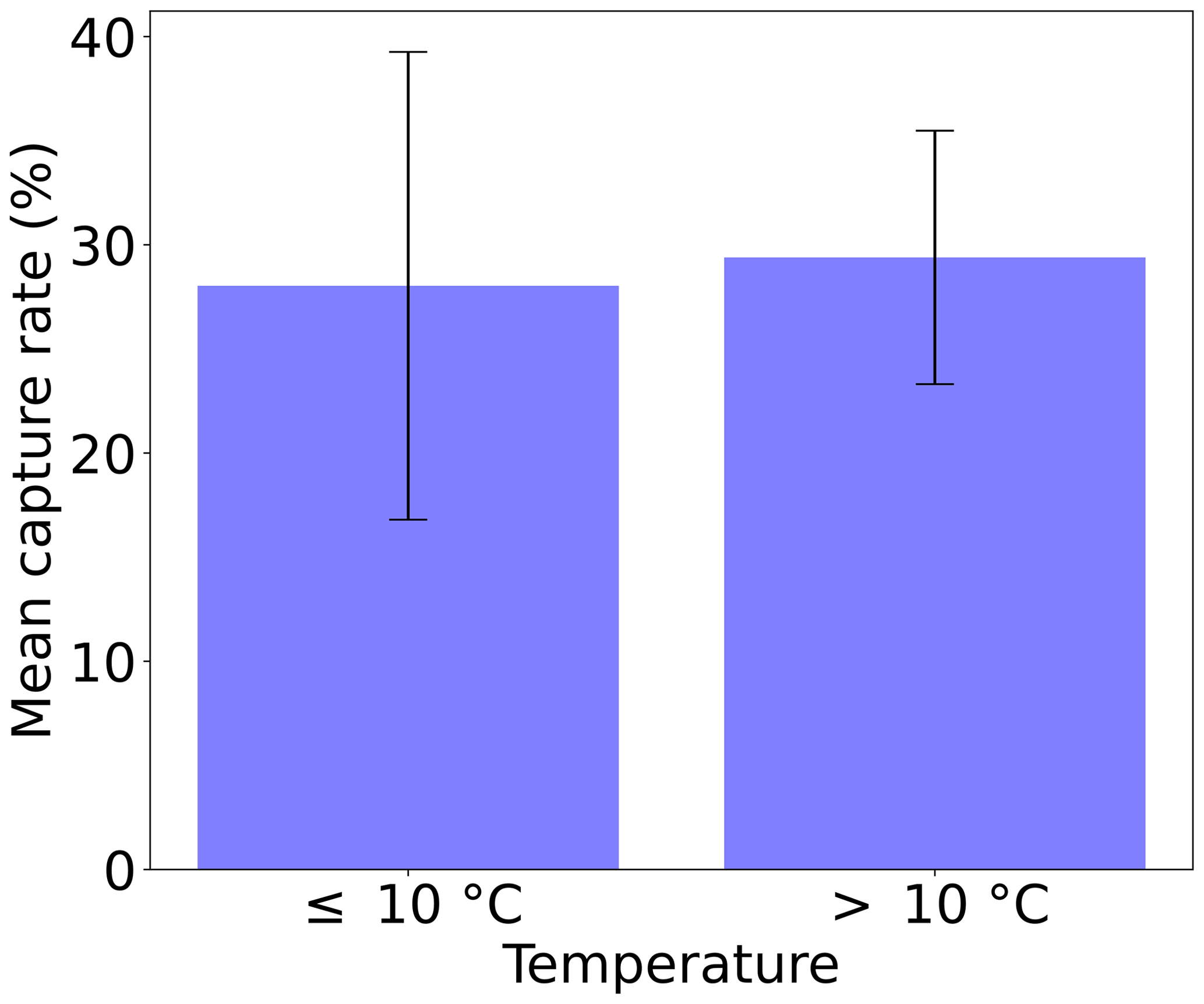
Temperature. The influence of temperature is investigated in Fig. 12 for low (≤ 10 °C) and high temperatures (> 10 °C). Ambient temperatures ranged from −7.3 to 28.2 °C during the different measurement campaigns. No significant difference was observed with an average CR of 28 % at low temperatures and of 29 % at high temperatures. The effects of ambient temperature and humidity are not expected to have an impact on the PS measurement itself, if the instrumentation used is either properly stored or can perform measurements under such conditions. Ambient temperature is expected to have an impact mainly on the passing vehicles and their exhaust after-treatment systems (Kwon et al., 2017; Ko et al., 2019).
3.3 Measurement campaign
In total, for the city measurement campaigns in Italy, Poland and Czechia, it was possible to collect technical data from authorities for 66 803 of the recorded vehicles. The measurement campaigns were carried out as part of the CARES project. The technical datasets collected were pseudo-anonymized to comply with the data protection regulations of the individual countries. Based on the technical datasets collected, we determined with our data analysis framework (see Sect. 2.2) the emissions of 22 160 vehicles. Measurements were conducted with our setup described in Sect. 2.1. Several instruments were used in the campaigns to measure BC, PN and NOx EFs. The newly developed BCT was used to measure BC and CO2, a custom-designed diffusion charger (Schriefl et al., 2020) measured PN concentrations and an ICAD (Airyx GmbH, Horbanski et al., 2019) was deployed for NOx and CO2 measurements. A schematic of the emission measurement setup can be found in the Supplement.
3.3.1 Fleet composition and capture rate
The measurements were carried out in city centers, which is also reflected in the vehicle fleet. The vehicle types were classified according to the vehicle categories of the United Nations Economic Commission for Europe (UNECE). The largest share of vehicles measured was passenger cars (84.1 %). Much smaller shares of L-type vehicles (1.4 %) and HDV and buses (0.8 %) were recorded (Fig. 13a, upper plot). We determined the CRs for the different vehicle categories to verify the ability to measure different vehicle types (Fig. 13a, lower plot). The highest CR was achieved for HDVs and buses (55 %), followed by passenger cars (22 %) and L-type vehicles (17 %). Previous PS studies (Dallmann et al., 2011, 2012) reported CRs for HDVs using top–down measurements from a bridge and a tunnel. In these studies CRs ranged from 12 % to 59 % for individual trucks and from 16 % to 44 % for groups of trucks. In general, it can be said that the CR depends on the exhaust flow rate of the vehicles. HDVs and buses have much greater exhaust flow rates than passenger cars or L-type vehicles. This is also reflected when looking at the average integrated exhaust plume of the different vehicle categories. The average integrated exhaust plume of HDVs and buses (947 ppm s CO2) was significantly higher than that of passenger cars (459 ppm s CO2) and L-type vehicles (374 ppm s CO2). A lower percentage of L-type vehicles is measured not only because of the smaller exhaust flow rate, but also because of the direction of the exhaust pipe. In contrast to HDVs, buses and passenger cars, the exhaust pipe for L-type vehicles often points upwards, which is disadvantageous when sampling from low heights. Looking at the distribution of the fuel type of the measured vehicles, a similar number of diesel (45.2 %) and petrol (46.5 %) vehicles were measured. A small share of CNG, LPG or bi-fuel (petrol or diesel + CNG or LPG, 2.6 %) was captured (Fig. 13b, upper plot). In contrast to the vehicle type, the CR is rather independent of the fuel type (Fig. 13b, lower plot). EFs were determined for 24 % of diesel vehicles, which is a slightly higher CR compared to 22 % of petrol vehicles. This is mainly due to the fact that vehicles with a larger engine displacement (e.g., trucks or buses) are mostly powered by diesel engines, while smaller vehicles are mostly equipped with petrol engines (e.g., L-type vehicles).
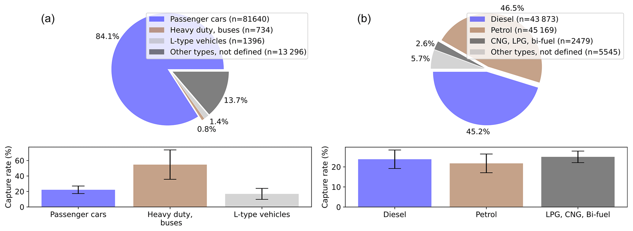
Figure 13Measured vehicle fleet split into vehicle categories (a) and fuel type (b). Capture rates for the different types are shown in the lower plots. The data contain multiple passes of the same vehicles.
3.3.2 Fleet emission characteristics
Fuel-based EFs (see Appendix A1) were determined for the measured vehicles using the technical vehicle data collected. Statistical evaluations were carried out for various vehicle categories and Euro emission standards (Figs. 14–16). Upper and lower whiskers represent the 97.5 and 2.5 percentile, respectively. The number of vehicles in each category is indicated by the numbers in the parentheses. Emissions from hybrid electric vehicles are included in the statistics. There are mainly two reasons for negative EFs. First, negative EFs result from low emitting vehicles where the background determined is higher than the emissions measured during the captured CO2 plume. Second, the emissions of other vehicles interfere with the measurement of the current vehicle.
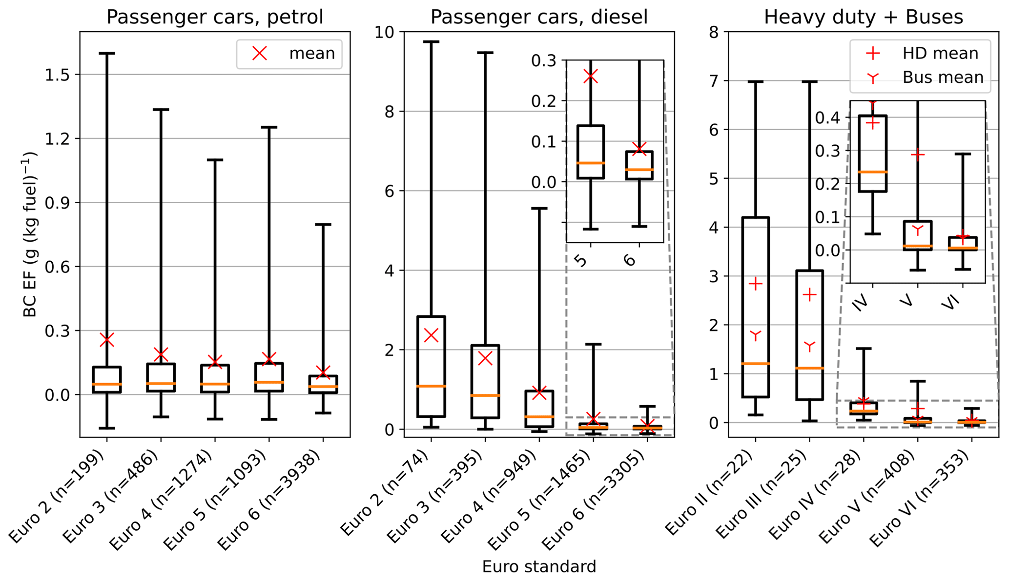
Figure 14Distribution of fuel-based BC EFs according to the Euro emission standard for different vehicle categories. Passenger cars are split into petrol- and diesel-powered vehicles. The numbers in parentheses represent the sample size.
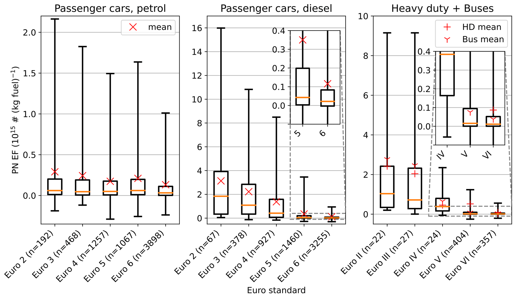
Figure 15Distribution of fuel-based PN EFs according to the Euro emission standard for different vehicle categories. PN measurements were performed for solid particles greater than 23 nm. Passenger cars are split into petrol- and diesel-powered vehicles. The numbers in parentheses represent the sample size.
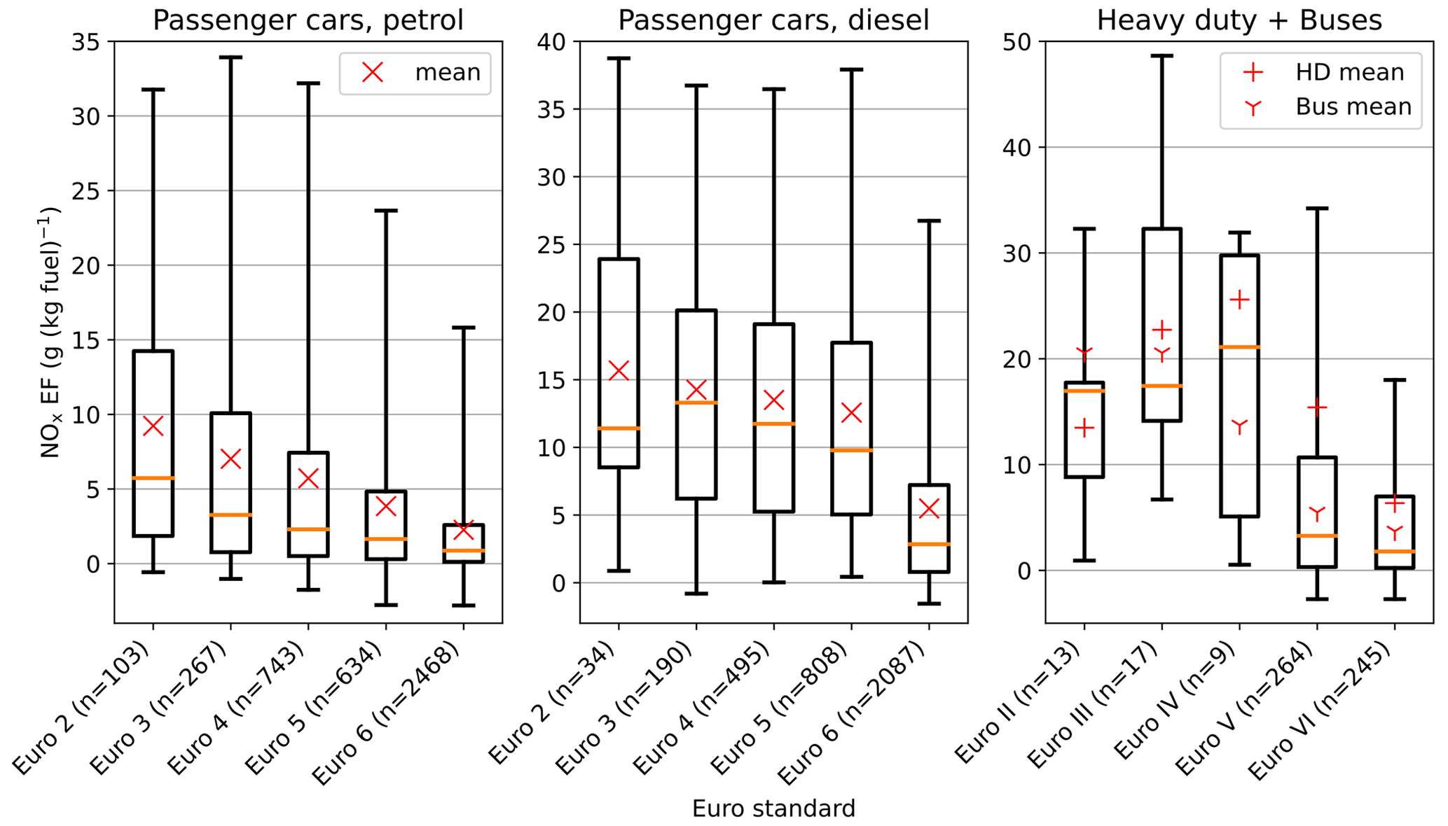
Figure 16Distribution of fuel-based NOx EFs according to the Euro emission standard for different vehicle categories. Passenger cars are split into petrol- and diesel-powered vehicles. The numbers in parentheses represent the sample size.
BC emissions from petrol-powered passenger cars (M1 category) decrease from Euro-2 to Euro-6 emission standards. The mean values decreased from 256 to 103 mg (kg fuel)−1, and the median values decreased from 57 to 37 mg (kg fuel)−1. For passenger cars with diesel engine, BC emissions decrease significantly with increasing Euro emission standards and decreasing vehicle age from 2.37 g (kg fuel)−1 (median: 1.08 g (kg fuel)−1) for Euro 2 down to 81 mg (kg fuel)−1 (median: 30 mg (kg fuel)−1) for Euro 6. This corresponds to a reduction by a factor of more than 30 from Euro 2 to Euro 6 on the median. The impact of the introduction of DPFs is evident from Euro 5 onwards. BC emissions from Euro-6 diesel vehicles are below those from Euro-6 petrol vehicles. Similar trends can be observed for BC emissions of HDVs and buses. The BC EFs of both HDVs and buses drop significantly from Euro III to Euro V. The buses measured were mainly well-maintained city-operated Euro-V and Euro-VI vehicles, with BC emissions even lower than those of Euro-6 passenger cars.
PN measurements were performed for particles larger than 23 nm (D50 cut-off at 23 nm) using a catalytic stripper to remove volatile compounds (Giechaskiel et al., 2014). PN and BC results agree well for the different vehicle categories and Euro emission standards, as only the solid particle fraction was measured (Fig. 15). The impact of the introduction of DPFs for diesel passenger cars is even more pronounced for PN than for BC. Median PN EFs decrease from Euro 2 to Euro 6 from 1842 to 22 × 1012 particles per kilogram fuel by a factor of more than 80. The greater reduction of PN compared to BC EFs can be related to DPF filtration efficiency, which depends on the particle size distribution (Yang et al., 2009; Rossomando et al., 2021). Vehicle exhaust PN consists mainly of a large number of small particles below 60 nm, while the main contributors to BC mass concentration are accumulation-mode particles (Giechaskiel et al., 2014). However, a shift towards smaller particle sizes caused by newer engine technologies must be taken into account.
NOx emission levels of petrol-powered passenger cars are steadily decreasing from Euro 2 to Euro 6 (Fig. 16). Median values decrease from 5.74 to 0.87 g (kg fuel)−1. The effects of “Dieselgate” are reflected in the NOx emissions of diesel passenger cars, which primarily affect Euro-5 and Euro-6 vehicles. NOx EFs stagnate for Euro-2 to Euro-5 vehicles, with median values ranging from 9.78 to 13.31 g (kg fuel)−1. For Euro-6 vehicles, NOx EFs decrease significantly with a median value of 2.85 g (kg fuel)−1. In contrast to BC and PN, NOx EFs for HDVs and buses are higher compared to emissions of passenger cars. This applies to all Euro classes. HDVs tend to have a higher mileage, which affects the deterioration of the vehicle's condition. In addition, intentional tampering of the NOx reduction system is believed to be more common in commercial vehicles than in private vehicles.
Table 3 compares average emissions of selected Euro emission standards from this study with previous open-path RES and PS studies. The average BC EFs from this study are compared with the PM EFs from other studies. BC can be assumed to be a subset of PM. For diesel vehicles, BC typically accounts for the largest share of PM emissions. This is especially the case for older Euro emission standards and for vehicles with defective DPF. The proportion of BC emissions for petrol vehicles is typically lower, except under specific conditions (Platt et al., 2017; Yang et al., 2019; Bessagnet et al., 2022). PN EFs are reported only for PS studies, because only rough estimates from open-path RES studies can be made for PN.
Table 3Comparison of average fuel-based BC, PM, PN and NOx EFs of this study with selected open-path RES and PS literature data. Emissions are ordered by vehicle category, fuel type and Euro emission standard. The BC, PM column shows either BC or PM EFs.
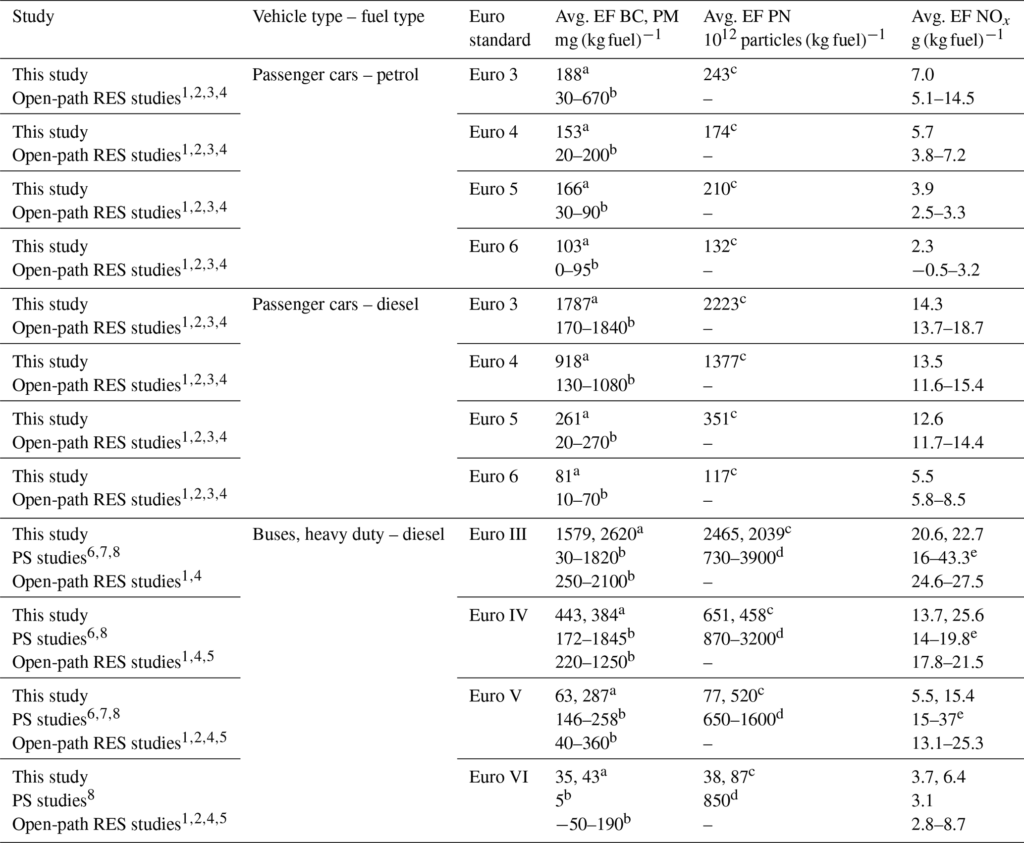
1 Hooftman et al. (2019), 2 Bernard et al. (2021), 3 Jerksjö et al. (2022), 4 Cha and Sjödin (2022), 5 Lee et al. (2022), 6 Hallquist et al. (2013), 7 Liu et al. (2019), 8 Zhou et al. (2020).
a BC, b PM, c PN > 23 nm, d PN > 5.6 nm, e NO EFs of Hallquist et al. (2013) were determined by open-path RES, NO2 measurements are estimated.
Average BC EFs from this study and PM EFs from open-path studies are in a similar range for petrol and diesel passenger cars. The average PM EFs reported from open-path RES studies are subject to a large variation. The measured emissions can vary widely depending on several factors such as fleet characteristics (e.g., vehicle type, manufacturer, mileage, age) or the measurement location. The average BC EFs determined in this study for Euro-5 and Euro-6 passenger cars are higher than those found in open-path RES studies. One reason for this can be the quantification limit of open-path RES instruments for PM measurements. Several studies pointed out difficulties in quantifying emissions of newer Euro emission standards, which was reflected in negative average EFs (Gruening et al., 2019; Cha and Sjödin, 2022; Jerksjö et al., 2022). The average NOx EFs from the selected open-path RES studies vary to a much smaller extent. The NOx EFs determined for passenger cars in this study agree well with values from the literature for almost all Euro emission standards given.
The EFs of HDVs and buses calculated in this study are compared with selected literature on both PS studies and open-path RES studies. The selected PS studies were conducted solely in Sweden. The BC EFs in this study and the PM EFs in studies from the literature are in similar ranges for Euro-III to Euro-V standards. Differences are mainly observed for Euro-VI HDVs. These can arise from differences in fleet characteristics or vehicle age, causing a deterioration of the exhaust after-treatment system. This could be particularly the case for newer Euro-VI HDVs, where 2–3 years between the studies can have a significant impact. Negative PM EFs reported by open-path RES studies can be due to limits in instrument accuracy similar to those for passenger cars. PN EFs for HDVs and buses reported in previous PS studies are generally higher than those reported in this study. This can be attributed to the different size characteristics of the PN instruments used. Particles larger than 5.6 nm were measured by Hallquist et al. (2013), Liu et al. (2019) and Zhou et al. (2020). In this study, the D50 cut-off was 23 nm (Schriefl et al., 2020). We performed solid particle number (SPN) measurements with a cut-off at 23 nm to comply with current emission regulations and to be able to relate the calculated EFs to official limits. The NOx EFs determined for HDVs and buses are in good agreement with data from the literature on PS and open-path RES studies. Similar to diesel passenger cars, the NOx EFs for HDVs and buses in this study are slightly lower compared to literature data for open-path RES studies. The NOx EFs from the literature on PS studies span a wide range, which can be due to differences in the vehicle exhaust after-treatment systems. In Hallquist et al. (2013), open-path RES data were used to determine NOx EFs. Which EFs are more accurate cannot be judged from the comparison, as several reasons influence the derived EFs such as measurement location, vehicle fleet, driving properties, environmental conditions, instrument characteristics or data analysis methods. A detailed comparison of our PS system with other simultaneous measurements will be part of a separate study (Knoll et al., 2024).
This paper presents a PS system capable of screening vehicle fleets largely independent of the vehicle type. Our approach enables the direct measurement of different particle metrics such as BC or PN as well as different gaseous compounds (e.g., NOx). In particular, PN is a relevant metric today with knowledge of the health effects of ultrafine particles (Oberdörster et al., 2005; Brook et al., 2010; Mannucci et al., 2015), but also concerning currently introduced emission legislation (Bainschab et al., 2020; Giechaskiel et al., 2021). Newly introduced Euro emission standards bring stringent requirements, where current open-path RES systems reach their quantification limits, especially for PM (Gruening et al., 2019; Cha and Sjödin, 2022; Jerksjö et al., 2022). Compared to commercial open-path RES systems, the installation of the PS measurement setup is relatively simple. The method is quite flexible in terms of where the sample extraction is performed and what instruments are used to measure the species of interest. We presented a comprehensive data analysis framework that is capable of processing emissions from thousands of vehicles. The core is the TUG-PDA, which determines and separates vehicle emissions down to a distance of 3 s between the vehicles, if appropriate instruments are used. We have shown that emissions from overlapping plumes can be measured with similar accuracy to when there is no overlap. As an application example, we presented the first results of measurement campaigns in three different European cities in which we made use of our PS method. We showed distributions of measured BC, PN and NOx EFs of different vehicle types and Euro emission standards. The results are in good agreement with relevant studies in the literature and show the potential for screening emissions of different vehicle types, including those meeting newly introduced emission standards.
We evaluated important impact factors influencing PS measurements that should be considered when planning and implementing PS campaigns. The most important influences are the following:
-
Instruments used for PS campaigns should be properly chosen (see Table 1). The response time, dynamic range and limit of detection are the most significant factors. The response time should be as low as possible (< 1–2 s). The dynamic range should be large enough to cover both low and high emitters. The limit of detection should be low enough to accurately determine the emissions from the evaluated species.
-
When selecting the measurement site, the traffic conditions must be taken into account. An ideal condition is a steady traffic flow with sufficient distance (≥ 3 s with appropriate instrumentation) between the vehicles to collect a high number of valid emission records. At the measurement site, the passing vehicles should be under considerable engine load. This can be either in appropriate traffic situations where vehicles accelerate (e.g., after crossing, slip road) or at roads with positive gradients.
-
The sampling should be performed as close to the exhaust source (tailpipe) as possible. The best results can be achieved if the sample extraction is performed from the middle of the road with the sampling tube directly attached to the road. When sampling from the side, the road width (smaller roads preferred) and the sampling height (as low as possible) have a significant influence on the CR. In addition, the position of the exhaust pipe of the fleet of interest should be examined in advance to determine the best sampling position.
-
The CR depends on the wind speed and direction. Windy conditions that transport the exhaust plume away from the sampling point have a negative effect on the CR. The influence of wind can be minimized by choosing an appropriate measurement location (e.g., street canyon). Other weather factors such as temperature or precipitation have negligible impact.
Future work will involve a detailed analysis of the BC, PN, and NOx emissions gathered. Several open questions will be addressed such as how PS measurements relate to those made by reference equipment such as PEMS or other RES methods (Knoll et al., 2024). Further development of the TUG-PDA could address improvements in the determination of BG for overlapping plumes (e.g., using a linear approximation between the start and end of the peak) or the use of adaptive thresholds and parameters depending on the measurement location. Another interesting aspect to investigate is the reproducibility and reliability of individual measurements. This is particularly important for the potential identification of high emitters. Commercial open-path RES systems are associated with a high degree of uncertainty when considering individual measurements (Huang et al., 2020; Qiu and Borken-Kleefeld, 2022). PS results indicate that single measurements are more reliable due to the longer measurement duration. It would be a significant step forward if this could be proven and applied in the future to identify individual high emitters.
A1 Emission ratio and fuel-based emission factor
Emissions of combustion-based vehicles are generally reported as EFs. In RES, fuel-based EFs are used to express emissions from the measured vehicles (Hansen and Rosen, 1990; Borken-Kleefeld and Dallmann, 2018; Bernard et al., 2018). Fuel-based emissions are expressed as a mass fraction of the emitted pollutant per mass of burned fuel. The amount of burned fuel is calculated based on the measured CO2 concentration of the passing vehicle by using the carbon mass balance method (Bishop et al., 1989; Hansen and Rosen, 1990; Stedman et al., 1992; Singer and Harley, 1996; Ban-Weiss et al., 2009; Hak et al., 2009) and under the assumption that the majority (> 90 %) of the carbon content in the fuel is oxidized to CO2 during the combustion process. By relating the measured pollutant P (e.g., BC, PN, NOx) to the measured CO2 concentration, an ER can first be calculated (Stedman et al., 1992; Hansen and Rosen, 1990). In our approach (see Eq. A1), we use different start (t1, t3) and stop times (t2, t4) for the pollutant and CO2 integration. Similarly, the BG values are determined independently (, ).
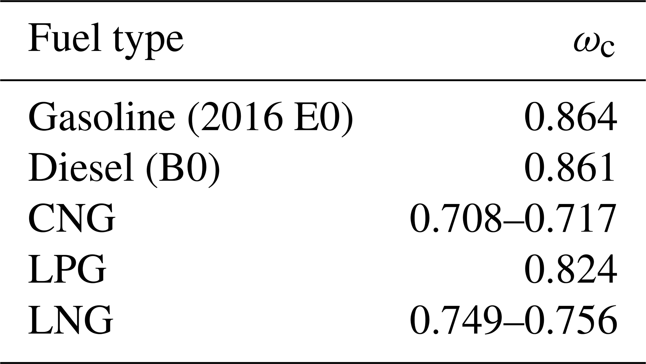
By multiplying the ER with the mass fraction of carbon in fuel, ωc, a fuel-based emission factor, EFfb (Ban-Weiss et al., 2009; Hak et al., 2009), can be calculated:
where ωc discriminates among different fuel types (see Table A1). Regarding PS measurements, the emission events last for several seconds. The measured concentrations of the pollutant and CO2 for one vehicle pass are commonly integrated and the results are related to each other. The start and stop times of the emission event define the integration intervals and these are represented by t1 and t1, respectively. The measured emissions are superimposed by BG concentrations of the different species in ambient air. For this reason, a BG correction is required, where t0 specifies the point of time from which the BG concentration is used. The BG is usually determined on the basis of the concentration at the integration starting point, t1. When plumes overlap or when impacts from other sources occur, this concentration may be underestimated.
A2 Distance-based emission factor
Fuel-based EFs do not distinguish between vehicles with different fuel consumption. Therefore, fuel-based EFs favor vehicles with higher fuel consumption. Distance-based EFs, on the contrary, include the fuel consumption and are, therefore, generally used to compare vehicle emissions (Bernard et al., 2018). However, distance-based EFs cannot be directly calculated in RES due to the snapshot measurement. An estimate can be calculated using the type-approval CO2 consumption () which is obtained from the vehicle technical information. The official CO2 emissions from passenger cars have been shown to differ increasingly from real-world emissions (Tietge et al., 2017). Therefore, a correction factor () including the real-world CO2 gap can be included according to Bernard et al. (2018). Making this assumption, a distance-based EF can be calculated as follows:
In a recent publication by Davison et al. (2020), a new approach was presented to calculate the distance-based EF in RES studies using the VSP. A good agreement was found between the outcome of their approach and validation measurements made with portable emission measurement systems (PEMS).
A3 Vehicle specific power
VSP is often used when performing emission modeling of combustion-based vehicles to estimate vehicle operating conditions. By using VSP, insights can be gained to estimate the engine load when a vehicle passes the measurement point. For example, this can be used to exclude vehicles with a small VSP (< −5 kW t−1) due to the disabled fuel injection in the engine (and therefore unexpected CO2 emissions) (Bernard et al., 2018). The VSP is defined according to Jimenez-Palacios (1999) by the sum of the relevant power variables related to the mass of the vehicle:
where EKin and EPot are the kinetic and the potential energies, respectively, v is the speed of the vehicle, FRol is the force from the rolling friction, FAero is the aerodynamic drag force, m is the mass of the vehicle, a is the vehicle acceleration, ϵ is the mass factor, g is the gravity of Earth, grade is the road gradient, CR is the coefficient of the rolling resistance, ρa is the density of ambient air, CD is the drag coefficient, A is the projected frontal area of the vehicle and vw is the headwind impacting the vehicle.
Figure B1 shows the detailed flowchart of the TUG-PDA.
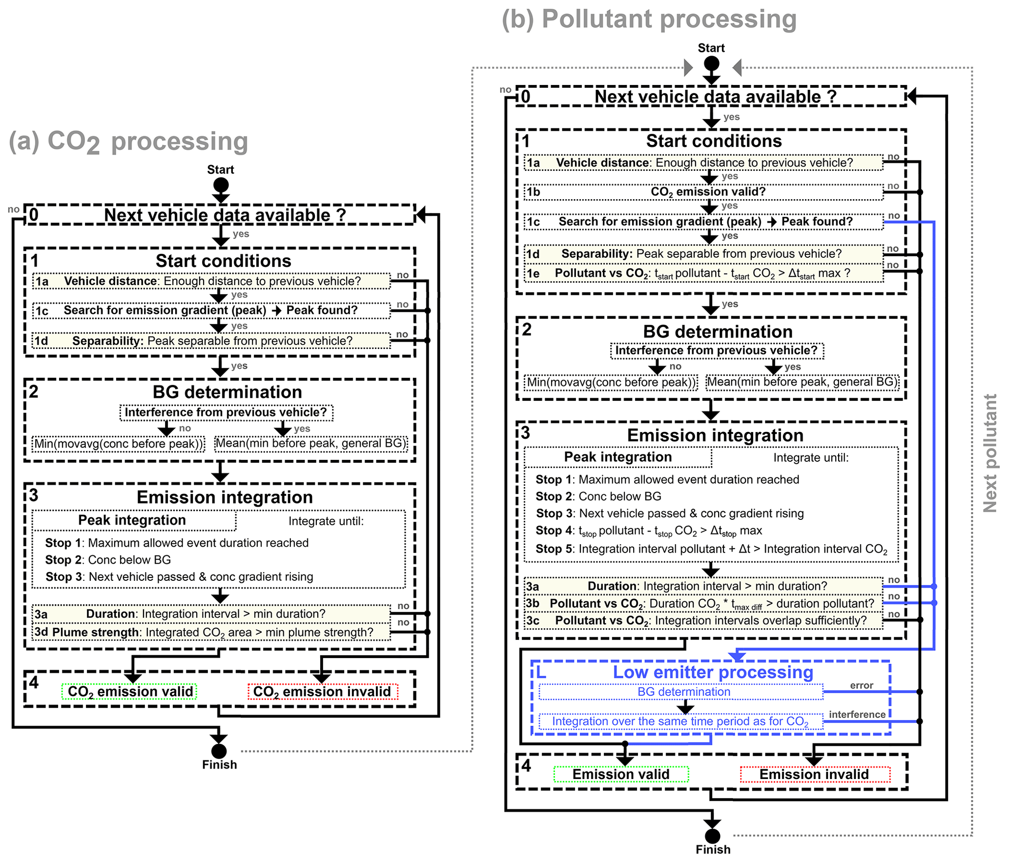
Figure B1Emission event processing – detailed flowcharts of the peak detection algorithm (TUG-PDA). CO2 and pollutant (e.g., BC, PN, NOx) emissions are processed separately. The algorithm is applied first to CO2 (a) and then to the individual pollutant emissions (b). The shaded boxes are QA conditions. The processing of low emitters is highlighted in blue. Specific processing steps are only applied to CO2 (3b) or to pollutants (1b, 1e, Stop 4, Stop 5, 3c, 3d, 3.1). Abbreviations: min – minimum, mov avg – moving average, conc – concentration, BG – background.
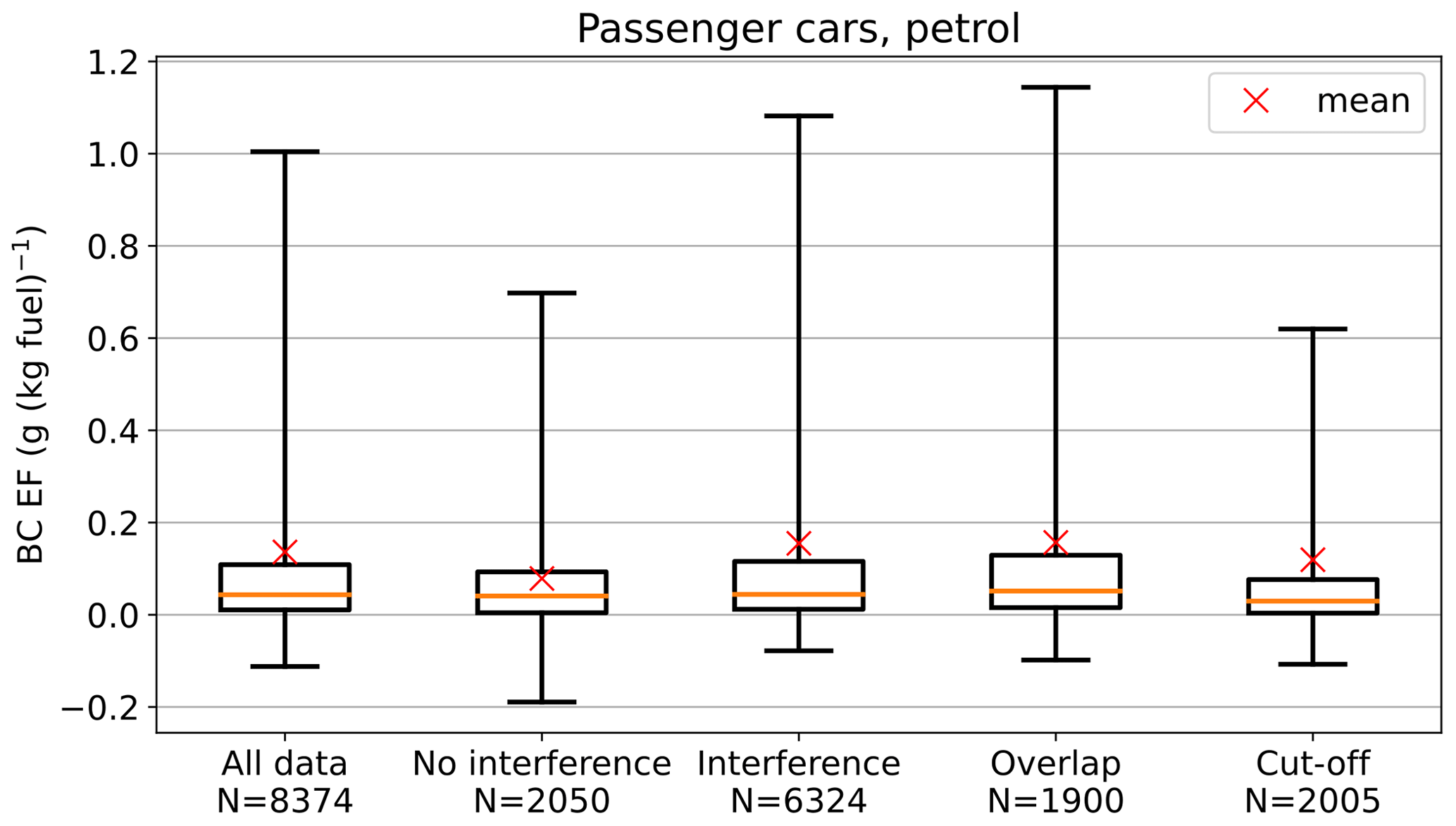
Figure C1Influence of interference (CO2 and BC) from other vehicles or pollution sources on the BC emission distributions determined with the TUG-PDA. Measured EFs of petrol-powered passenger cars are used for comparison. Interference data include both the overlapping plumes and the plume cut-offs (interference = overlap and/or cut-off).
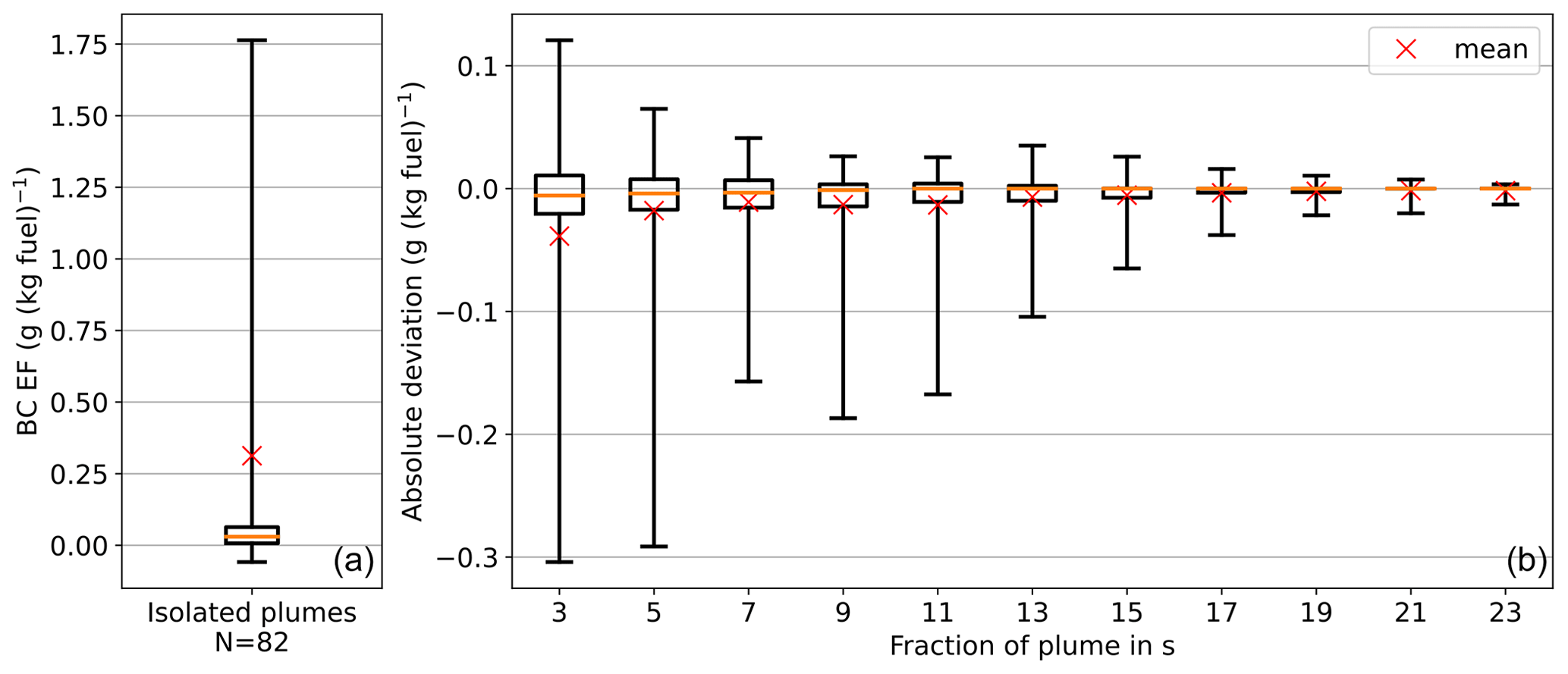
Figure C2Deviation when using only a fraction of the plume to calculate EFs compared to using the entire plume. (a) Distribution of EFs of plumes without interference from other vehicles. (b) Deviation from full plume (25 s) using only fractions between 3 and 23 s.
Figure C1 shows the influence of interference, but it additionally includes the superposition of the measured BC emissions to the superposition of CO2 emissions. The emission distributions are separated in the same manner as in Fig. 6 into the measured CO2 plumes with and without interference from other vehicles or pollution sources. Compared to Fig. 6, measured CO2 plumes with interference are slightly higher compared to plumes without interference. This is due to the fact that most of the BC superimposed vehicle emissions are contained in the inference datasets. These are mainly vehicles with higher emissions, as BC peaks could be detected.
Figure C2 shows how accurate EFs can be calculated when using only a fraction of the plume. Therefore, the algorithm selected 82 plumes that were not affected by emissions from other vehicles. The average plume length of this selection was 18 s and 30 of the plumes were longer than 25 s. The full distribution using the algorithm's defined maximum plume length of 25 s is shown in Fig. C2a. Figure C2b shows the deviation from the full plume when only a fraction between 3 and 23 s is used. The median deviation is maximum at 3 s with 27 % and decreases steadily with increasing plume fraction.
The code of the software framework is available at: https://gitlab.com/tug-ems/point-sampling.git (Knoll, 2024).
Measurement data are available in the CARES database for the PS measurements and on request to the authors.
The supplement related to this article is available online at: https://doi.org/10.5194/amt-17-2481-2024-supplement.
The conceptualization was done by MK and AB. The measurements were conducted by MK, HJ and CS. The methodology and investigations were completed by MK, MP, HJ, CS, DP and AB. The software and material preparation were done by MK. MK drafted the original manuscript, which was reviewed by MP, HJ, CS, DP and AB. The project was supervised at Graz University of Technology by AB.
The contact author has declared that none of the authors has any competing interests.
Publisher's note: Copernicus Publications remains neutral with regard to jurisdictional claims made in the text, published maps, institutional affiliations, or any other geographical representation in this paper. While Copernicus Publications makes every effort to include appropriate place names, the final responsibility lies with the authors.
We want to thank Åke Sjödin (IVL) for the great support during the whole project. We thank Yoann Bernard (ICCT) for the organization of the overall campaigns. We want to thank Åsa Hallquist (IVL) for the support with the PS measurements. We thank Norbert Ligterink, Thomas Frateur, Quinn Vroom and Jan Pieter Lollinga from TNO for the support during the characterization experiments and the Prague campaign and for providing an ANPR camera system for all measurement campaigns. We thank David Carslaw and Naomi Farren for their support during the project. Many thanks to Simone Casadei and Tommaso Rossi from Innovhub and Silvia Moroni and Marco Bedogni from AMAT for the organization and their help during the Milan campaign. We want to thank ZTP Krakow and Bartosz Piłat for the support during the Krakow campaign. Many thanks to Michal Vojtíšek and Martin Pechout for their help during the Krakow and Prague campaigns. We thank Jens Borken-Kleefeld for the continuous support during the project. Finally, we want to thank Sitaram Stepponat and Andreas Steiner for their continuous support and discussions during the project, especially for the preparation of the measurement campaigns.
This research has been supported by the TU Graz Open Access Publishing Fund and the EU H2020 project CARES (grant no. 814966).
This paper was edited by Jean-Philippe Putaud and reviewed by two anonymous referees.
Bainschab, M., Schriefl, M. A., and Bergmann, A.: Particle number measurements within periodic technical inspections: A first quantitative assessment of the influence of size distributions and the fleet emission reduction, Atmospheric Environment: X, 8, 100095, https://doi.org/10.1016/j.aeaoa.2020.100095, 2020. a, b, c, d
Ban-Weiss, G. A., McLaughlin, J. P., Harley, R. A., Lunden, M. M., Kirchstetter, T. W., Kean, A. J., Strawa, A. W., Stevenson, E. D., and Kendall, G. R.: Long-term changes in emissions of nitrogen oxides and particulate matter from on-road gasoline and diesel vehicles, Atmos. Environ., 42, 220–232, https://doi.org/10.1016/j.atmosenv.2007.09.049, 2008. a, b, c
Ban-Weiss, G. A., Lunden, M. M., Kirchstetter, T. W., and Harley, R. A.: Measurement of black carbon and particle number emission factors from individual heavy-duty trucks, Environ. Sci. Technol., 43, 1419–1424, https://doi.org/10.1021/es8021039, 2009. a, b, c, d, e
Ban-Weiss, G. A., Lunden, M. M., Kirchstetter, T. W., and Harley, R. A.: Size-resolved particle number and volume emission factors for on-road gasoline and diesel motor vehicles, J. Aerosol Sci., 41, 5–12, https://doi.org/10.1016/j.jaerosci.2009.08.001, 2010. a, b
Bernard, Y., Tietge, U., German, J., and Muncrief, R.: White paper: Determination of real-world emissions from passenger vehicles using remote sensing data, Tech. rep., International Council on Clean Transportation, https://www.trueinitiative.org/data/publications/determination-of-real-world-emissions-from-passenger-vehicles-using-remote-sensing-data (last access: 10 April 2024), 2018. a, b, c, d, e, f
Bernard, Y., Dallmann, T., Lee, K., Rintanen, I., and Tietge, U.: Evaluation of real-world vehicle emissions in Brussels, Tech. rep., International Council on Clean Transportation, Journal of Aerosol Science, https://www.trueinitiative.org/media/792040/true-brussels-report.pdf (last access: 10 April 2024), 2021. a
Bessagnet, B., Allemand, N., Putaud, J.-P., Couvidat, F., André, J.-M., Simpson, D., Pisoni, E., Murphy, B., and Thunis, P.: Emissions of Carbonaceous Particulate Matter and Ultrafine Particles from Vehicles—A Scientific Review in a Cross-Cutting Context of Air Pollution and Climate Change, Appl. Sci., 2022, 3623, https://doi.org/10.3390/app12073623, 2022. a
Bishop, G. A., Starkey, J. R., Ihlenfeldt, A., Williams, W. J., and Stedman, D. H.: IR Long-Path Photometry A Remote Sensing Tool for Automobile Emissions, Anal. Chem., 61, 671A–677A, https://doi.org/10.1021/ac00185a746, 1989. a, b, c
Bishop, G. A., Hottor-Raguindin, R., Stedman, D. H., McClintock, P., Theobald, E., Johnson, J. D., Lee, D. W., Zietsman, J., and Misra, C.: On-road heavy-duty vehicle emissions monitoring system, Environ. Sci. Technol., 49, 1639–1645, https://doi.org/10.1021/es505534e, 2015. a, b
Borken-Kleefeld, J. and Dallmann, T.: White paper: Remote sensing of motor vehicle exhaust emissions, Tech. rep., International Council on Clean Transportation, https://theicct.org/publication/remote-sensing-of-motor-vehicle-exhaust-emissions (last access: 10 April 2024), 2018. a, b
Boveroux, F., Cassiers, S., Buekenhoudt, P., Chavatte, L., Meyer, P. D., Jeanmart, H., Verhelst, S., and Contino, F.: Feasibility study of a new test procedure to identify high emitters of particulate matter during periodic technical inspection, SAE Technical Papers, SAE International, United States, https://doi.org/10.4271/2019-01-1190, 2019. a
Brook, R. D., Rajagopalan, S., Pope, C. A., Brook, J. R., Bhatnagar, A., Diez-Roux, A. V., Holguin, F., Hong, Y., Luepker, R. V., Mittleman, M. A., Peters, A., Siscovick, D., Smith, S. C., Whitsel, L., and Kaufman, J. D.: Particulate matter air pollution and cardiovascular disease: An update to the scientific statement from the american heart association, Circulation, 121, 2331–2378, https://doi.org/10.1161/CIR.0b013e3181dbece1, 2010. a, b
Burgard, D. A., Bishop, G. A., Stadtmuller, R. S., Dalton, T. R., and Stedman, D. H.: Spectroscopy Applied to On-Road Mobile Source Emissions, Appl. Spectrosc., 60, 135A–148A, https://doi.org/10.1366/000370206777412185, 2006. a
Burtscher, H., Lutz, T., and Mayer, A.: A New Periodic Technical Inspection for Particle Emissions of Vehicles, Emission Control Science and Technology, 5, 279–287, https://doi.org/10.1007/s40825-019-00128-z, 2019. a
Cha, Y. and Sjödin, A.: Remote Sensing Measurements of Vehicle Emissions in Sarajevo, Tech. rep., IVL Swedish Environmental Research Institute, https://www.ivl.se/download/18.5ae47fd818530c6f06012a7c/1680696264314/C727.pdf (last access: 10 April 2024), 2022. a, b, c, d
Chu, M., Brimblecombe, P., Wei, P., Liu, C. H., Du, X., Sun, Y., Yam, Y. S., and Ning, Z.: Kerbside NOx and CO concentrations and emission factors of vehicles on a busy road, Atmos. Environ., 271, 118878, https://doi.org/10.1016/j.atmosenv.2021.118878, 2022. a
Dallmann, T. R., Harley, R. A., and Kirchstetter, T. W.: Effects of diesel particle filter retrofits and accelerated fleet turnover on drayage truck emissions at the port of Oakland, Environ. Sci. Technol., 45, 10773–10779, https://doi.org/10.1021/es202609q, 2011. a, b, c, d
Dallmann, T. R., Demartini, S. J., Kirchstetter, T. W., Herndon, S. C., Onasch, T. B., Wood, E. C., and Harley, R. A.: On-road measurement of gas and particle phase pollutant emission factors for individual heavy-duty diesel trucks, Environ. Sci. Technol., 46, 8511–8518, https://doi.org/10.1021/es301936c, 2012. a, b
Dallmann, T. R., Kirchstetter, T. W., Demartini, S. J., and Harley, R. A.: Quantifying on-road emissions from gasoline-powered motor vehicles: Accounting for the presence of medium- and heavy-duty diesel trucks, Environ. Sci. Technol., 47, 13873–13881, https://doi.org/10.1021/es402875u, 2013. a
Dallmann, T. R., Onasch, T. B., Kirchstetter, T. W., Worton, D. R., Fortner, E. C., Herndon, S. C., Wood, E. C., Franklin, J. P., Worsnop, D. R., Goldstein, A. H., and Harley, R. A.: Characterization of particulate matter emissions from on-road gasoline and diesel vehicles using a soot particle aerosol mass spectrometer, Atmos. Chem. Phys., 14, 7585–7599, https://doi.org/10.5194/acp-14-7585-2014, 2014. a
Davison, J., Bernard, Y., Borken-Kleefeld, J., Farren, N. J., Hausberger, S., Åke Sjödin, Tate, J. E., Vaughan, A. R., and Carslaw, D. C.: Distance-based emission factors from vehicle emission remote sensing measurements, Sci. Total Environ., 739, 139688, https://doi.org/10.1016/j.scitotenv.2020.139688, 2020. a, b
EEA: Air quality in Europe: 2017 report, Tech. rep., European Environment Agency and European Topic Centre on Air Pollution and Climate Change Mitigation (ETC/ACM), Publications Office of the European Union, Luxembourg, 2017. a
Farren, N. J., Schmidt, C., Juchem, H., Pöhler, D., Wilde, S. E., Wagner, R. L., Wilson, S., Shaw, M., and Carslaw, D. C.: Emission ratio determination from road vehicles using a range of remote emission sensing techniques, Sci. Total Environ., 875, 162621, https://doi.org/10.1016/j.scitotenv.2023.162621, 2023. a
Giechaskiel, B., Arndt, M., Schindler, W., Bergmann, A., Silvis, W., and Drossinos, Y.: Sampling of Non-Volatile Vehicle Exhaust Particles: A Simplified Guide, SAE Int. J. Engines, 5, 379–399, https://doi.org/10.4271/2012-01-0443, 2012. a
Giechaskiel, B., Maricq, M., Ntziachristos, L., Dardiotis, C., Wang, X., Axmann, H., Bergmann, A., and Schindler, W.: Review of motor vehicle particulate emissions sampling and measurement: From smoke and filter mass to particle number, J. Aerosol Sci., 67, 48–86, https://doi.org/10.1016/j.jaerosci.2013.09.003, 2014. a, b
Giechaskiel, B., Lähde, T., Suarez-Bertoa, R., Valverde, V., and Clairotte, M.: Comparisons of laboratory and on-road type-approval cycles with idling emissions. Implications for periodical technical inspection (PTI) sensors, Sensors, 20, 1–18, https://doi.org/10.3390/s20205790, 2020. a
Giechaskiel, B., Melas, A., Martini, G., and Dilara, P.: Overview of vehicle exhaust particle number regulations, Processes, 9, 2216, https://doi.org/10.3390/pr9122216, 2021. a, b, c
Gruening, C., Bonnel, P., Clairotte, M., Giechaskiel, B., Valverde, V., Zardini, A., and Carriero, M.: Potential of Remote Sensing Devices (RSDs) to screen vehicle emissions Assessment of RSD measurement performance, JRC Technical Reports, Joint Research Centre, https://doi.org/10.2760/277092, 2019. a, b, c
Hak, C. S., Hallquist, M., Ljungström, E., Svane, M., and Pettersson, J. B.: A new approach to in-situ determination of roadside particle emission factors of individual vehicles under conventional driving conditions, Atmos. Environ., 43, 2481–2488, https://doi.org/10.1016/j.atmosenv.2009.01.041, 2009. a, b, c, d, e, f, g, h, i, j
Hallquist, Å. M., Jerksjö, M., Fallgren, H., Westerlund, J., and Sjödin, Å.: Particle and gaseous emissions from individual diesel and CNG buses, Atmos. Chem. Phys., 13, 5337–5350, https://doi.org/10.5194/acp-13-5337-2013, 2013. a, b, c, d, e, f
Hansen, A. D. and Rosen, H.: Individual measurements of the emission factor of aerosol black carbon in automobile plumes, J. Air Waste Manage., 40, 1654–1657, https://doi.org/10.1080/10473289.1990.10466812, 1990. a, b, c, d
Hooftman, N., Norbert, L., and Akshay, B.: Analysis of the 2019 Flemish remote sensing campaign Final report, Tech. rep., Departement Omgeving, Vlaams Planbureau voor Omgeving, Brussel, https://publications.tno.nl/publication/34638150/2gBdxC/hooftman-2020-analysis.pdf (last access: 10 April 2024), 2019. a
Horbanski, M., Pöhler, D., Lampel, J., and Platt, U.: The ICAD (iterative cavity-enhanced DOAS) method, Atmos. Meas. Tech., 12, 3365–3381, https://doi.org/10.5194/amt-12-3365-2019, 2019. a
Huang, Y., Surawski, N. C., Yam, Y. S., Lee, C. K., Zhou, J. L., Organ, B., and Chan, E. F.: Re-evaluating effectiveness of vehicle emission control programmes targeting high-emitters, Nat. Sustain., 3, 904–907, https://doi.org/10.1038/s41893-020-0573-y, 2020. a
Janhäll, S. and Hallquist, M.: A novel method for determination of size-resolved, submicrometer particle traffic emission factors, Environ. Sci. Technol., 39, 7609–7615, https://doi.org/10.1021/es048208y, 2005. a
Jerksjö, M., Åke Sjödin, Merelli, L., Varella, R., and Sandström-Dahl, C.: Remote emission sensing compared with other methods to measure in-service conformity of light-duty vehicles, Tech. rep., IVL Swedish Environmental Research Institute, AVL MTC, Stockholm, Sweden, https://www.ivl.se/english/ivl/publications/publications/ remote-emission-sensing-compared-with-other-methods-to-measure-in-service-conformity-of-light-duty-vehicles-on-behalf-of-the-swedish-innovation-agency-and-the-swedish-transport-administration.html (last access: 10 April 2024), 2022. a, b, c, d
Ježek, I., Drinovec, L., Ferrero, L., Carriero, M., and Močnik, G.: Determination of car on-road black carbon and particle number emission factors and comparison between mobile and stationary measurements, Atmos. Meas. Tech., 8, 43–55, https://doi.org/10.5194/amt-8-43-2015, 2015. a, b, c, d
Jimenez-Palacios, J. L.: Understanding and Quantifying Motor Vehicle Emissions with Vehicle Specific Power and TILDAS Remote Sensing, PhD thesis, Massachusetts Institute of Technology, 1999. a
JRC: JEC Well-To-Wheels report v5, Tech. rep., Joint Research Center, European Commission, https://doi.org/10.2760/100379, 2020. a
Järvinen, A., Timonen, H., Karjalainen, P., Bloss, M., Simonen, P., Saarikoski, S., Kuuluvainen, H., Kalliokoski, J., Maso, M. D., Niemi, J. V., Keskinen, J., and Rönkkö, T.: Particle emissions of Euro VI, EEV and retrofitted EEV city buses in real traffic, Environ. Pollut., 250, 708–716, https://doi.org/10.1016/j.envpol.2019.04.033, 2019. a
Kelly, C., Fawkes, J., Habermehl, R., de Ferreyro Monticelli, D., and Zimmerman, N.: PLUME Dashboard: A free and open-source mobile air quality monitoring dashboard, Environ. Modell. Softw., 160, 105600, https://doi.org/10.1016/j.envsoft.2022.105600, 2023. a
Knoll, A., Lang, B., and Bergmann, A.: Performance of Black Carbon Instruments for Extractive Remote Emission Sensing, AAAR conference 2021, 18–22 October 2021, abstract no. 9IM.2, https://aaarabstracts.com/2021/AbstractBook.pdf (last access: 10 April 2024), 2021. a, b
Knoll, M.: GitLab repository of a basic version of the Point sampling post-processing framework, GitLab [code], https://gitlab.com/tug-ems/point-sampling.git, last access: 10 April 2024. a
Knoll, M., Penz, M., Schmidt, C., Pöhler, D., Rossi, T., Casadei, S., Bernard, Y., Hallquist, A. M., Sjödin, A., and Bergmann, A.: Evaluation of the point sampling method and inter-comparison with remote emission sensing systems for screening real world car emissions, Sci. Total Environ., in press, https://doi.org/10.1016/j.scitotenv.2024.171710, 2024. a, b, c
Ko, J., Myung, C. L., and Park, S.: Impacts of ambient temperature, DPF regeneration, and traffic congestion on NOx emissions from a Euro 6-compliant diesel vehicle equipped with an LNT under real-world driving conditions, Atmos. Environ., 200, 1–14, https://doi.org/10.1016/j.atmosenv.2018.11.029, 2019. a
Kulkarni, P., Baron, P. A., and Willeke, K.: Aerosol measurement: principles, techniques, and applications, John Wiley & Sons, Inc., Hoboken, New Jersey, ISBN 978-0-470-38741-2, 2011. a
Kwon, S., Park, Y., Park, J., Kim, J., Choi, K. H., and Cha, J. S.: Characteristics of on-road NOx emissions from Euro 6 light-duty diesel vehicles using a portable emissions measurement system, Sci. Total Environ., 576, 70–77, https://doi.org/10.1016/j.scitotenv.2016.10.101, 2017. a
Lee, K., Bernard, Y., Dallmann, T., Tietge, U., Pniewska, I., and Rintanen, I.: Evaluation of real-world vehicle emissions in Warsaw, Tech. rep., International Council on Clean Transportation, https://theicct.org/wp-content/uploads/2022/04/true-warsaw-emissions-apr22.pdf (last access: 10 April 2024), 2022. a
Liu, Q., Å. M. Hallquist, Fallgren, H., Jerksjö, M., Jutterström, S., Salberg, H., Hallquist, M., Breton, M. L., Pei, X., Pathak, R. K., Liu, T., Lee, B., and Chan, C. K.: Roadside assessment of a modern city bus fleet: Gaseous and particle emissions, Atmospheric Environment: X, 3, 100044, https://doi.org/10.1016/j.aeaoa.2019.100044, 2019. a, b, c, d, e, f
Mannucci, P. M., Harari, S., Martinelli, I., and Franchini, M.: Effects on health of air pollution: a narrative review, Intern. Emerg. Med., 10, 657–662, https://doi.org/10.1007/s11739-015-1276-7, 2015. a, b
Melas, A., Selleri, T., Suarez-Bertoa, R., and Giechaskiel, B.: Evaluation of solid particle number sensors for periodic technical inspection of passenger cars, Sensors, 21, 8325, https://doi.org/10.3390/s21248325, 2021. a
Meyer, M., Bernard, Y., German, J., and Dallmann, T.: Reassessment of Excess NOx from European Diesel Cars following the Court of Justice of the European Union Rulings, Tech. rep., International Council on Clean Transportation Europe, Berlin,, https://theicct.org/wp-content/uploads/2023/03/dieselgate-emissions-diesel-cars-Europe-mar23.pdf (last access: 10 April 2024), 2023. a
Mock, P. and German, J.: The future of vehicle emissions testing and compliance how to align regulatory requirements, customer expectations, and environmental performance in the european union, Tech. rep., White paper, International Council on Clean Transportation Europe, Berlin,, https://theicct.org/wp-content/uploads/2021/06/ICCT_future-vehicle-testing_20151123.pdf (last access: 10 April 2024), 2015. a
Moosmüller, H., Mazzoleni, C., Barber, P. W., Kuhns, H. D., Keislar, R. E., and Watson, J. G.: On-Road Measurement of Automotive Particle Emissions by Ultraviolet Lidar and Transmissometer: Instrument, Environ. Sci. Technol., 37, 4971–4978, https://doi.org/10.1021/es034443p, 2003. a
Oberdörster, G., Oberdörster, E., and Oberdörster, J.: Nanotoxicology: An Emerging Discipline Evolving from Studies of Ultrafine Particles, Environ. Health Persp., 113, 823–839, https://doi.org/10.1289/ehp.7339, 2005. a, b
Park, S. S., Kozawa, K., Fruin, S., Mara, S., Hsu, Y. K., Jakober, C., Winer, A., and Herner, J.: Emission Factors for High-Emitting Vehicles Based on On-Road Measurements of Individual Vehicle Exhaust with a Mobile Measurement Platform, J. Air Waste Manage., 61, 1046–1056, https://doi.org/10.1080/10473289.2011.595981, 2011. a
Platt, S. M., Haddad, I. E., Pieber, S. M., Zardini, A. A., Suarez-Bertoa, R., Clairotte, M., Daellenbach, K. R., Huang, R. J., Slowik, J. G., Hellebust, S., Temime-Roussel, B., Marchand, N., Gouw, J. D., Jimenez, J. L., Hayes, P. L., Robinson, A. L., Baltensperger, U., Astorga, C., and Prévôt, A. S.: Gasoline cars produce more carbonaceous particulate matter than modern filter-equipped diesel cars, Sci. Rep.-UK, 7, 4926, https://doi.org/10.1038/s41598-017-03714-9, 2017. a
Preble, C. V., Dallmann, T. R., Kreisberg, N. M., Hering, S. V., Harley, R. A., and Kirchstetter, T. W.: Effects of Particle Filters and Selective Catalytic Reduction on Heavy-Duty Diesel Drayage Truck Emissions at the Port of Oakland, Environ. Sci. Technol., 49, 8864–8871, https://doi.org/10.1021/acs.est.5b01117, 2015. a, b
Preble, C. V., Cados, T. E., Harley, R. A., and Kirchstetter, T. W.: In-Use Performance and Durability of Particle Filters on Heavy-Duty Diesel Trucks, Environ. Sci. Technol., 52, 11913–11921, https://doi.org/10.1021/acs.est.8b02977, 2018. a, b, c
Pöhler, D., Engel, T., Roth, U., Reber, J., Horbanski, M., Lampel, J., and Platt, U.: NOx RDE measurements with Plume Chasing-Validation, detection of high emitters and manipulated SCR systems, in: Proceedings of the 23rd Transport and Air Pollution (TAP) conference, Part II, Thessaloniki, Greece, 15–17 May 2019, edited by: Karamountzou, G., Fontaras, G., Mamarikas, S., and Ntziachristos, L., Publications Office, https://doi.org/10.2760/978944, 2020. a
Qiu, M. and Borken-Kleefeld, J.: Using snapshot measurements to identify high-emitting vehicles, Environ. Res. Lett., 17, 044045, https://doi.org/10.1088/1748-9326/ac5c9e, 2022. a
Rossomando, B., Meloni, E., de Falco, G., Sirignano, M., Arsie, I., and Palma, V.: Experimental characterization of ultrafine particle emissions from a light-duty diesel engine equipped with a standard DPF, P. Combust. Inst., 38, 5695–5702, https://doi.org/10.1016/j.proci.2020.09.011, 2021. a
Rönkkö, T., Saarikoski, S., Kuittinen, N., Karjalainen, P., Keskinen, H., Järvinen, A., Mylläri, F., Aakko-Saksa, P., and Timonen, H.: Review of black carbon emission factors from different anthropogenic sources, Environ. Res. Lett., 18, 033004, https://doi.org/10.1088/1748-9326/acbb1b, 2023. a
Salimbene, O., Morreale, S., and Pilla, F.: Health Risk Assessment and Black Carbon: State of Art and new Prospectives, in: Air Pollution XXIX, WITPress, 252, 149–159, https://doi.org/10.2495/AIR210141, 2021. a
Schriefl, M. A., Nishida, R. T., Knoll, M., Boies, A. M., and Bergmann, A.: Characterization of particle number counters based on pulsed-mode diffusion charging, Aerosol Sci. Techn., 54, 772–789, https://doi.org/10.1080/02786826.2020.1724257, 2020. a, b
Singer, B. C. and Harley, R. A.: A Fuel-Based Motor Vehicle Emission Inventory, J. Air Waste Manage., 46, 581–593, https://doi.org/10.1080/10473289.1996.10467492, 1996. a
Singleton, F.: The Beaufort scale of winds – Its relevance, and its use by sailors, Weather, 63, 37–41, https://doi.org/10.1002/wea.153, 2008. a
Stedman, D. H., Bishop, G. A., Guenther, P. L., Peterson, J. E., and Beaton, S. P.: Remote Sensing of On-Road Vehicle Emissions, University of Denver, Digital Commons @ DU, https://digitalcommons.du.edu/feat_publications (last access: 10 April 2024), 1992. a, b, c
Sugrue, R. A., Preble, C. V., and Kirchstetter, T. W.: Comparing the use of high-to low-cost black carbon and carbon dioxide sensors for characterizing on-road diesel truck emissions, Sensors, 20, 1–18, https://doi.org/10.3390/s20236714, 2020. a, b, c
Tietge, U., Mock, P., German, J., Bandivadekar, A., and Ligterink, N.: From Laboratory to road. A 2017 update of official and “real-world” fuel consumption and CO2 values for passenger cars in Europe, Tech. rep., White paper, International Council on Clean Transportation Europe, Berlin, https://theicct.org/sites/default/files/publications/Lab-to-road-2017_ICCT-white%20paper_06112017_vF.pdf (last access: 10 April 2024), 2017. a
Wang, H., Wu, Y., Zhang, K. M., Zhang, S., Baldauf, R. W., Snow, R., Deshmukh, P., Zheng, X., He, L., and Hao, J.: Evaluating mobile monitoring of on-road emission factors by comparing concurrent PEMS measurements, Sci. Total Environ., 736, 139507, https://doi.org/10.1016/j.scitotenv.2020.139507, 2020. a
Wang, J. M., Jeong, C.-H., Zimmerman, N., Healy, R. M., Wang, D. K., Ke, F., and Evans, G. J.: Plume-based analysis of vehicle fleet air pollutant emissions and the contribution from high emitters, Atmos. Meas. Tech., 8, 3263–3275, https://doi.org/10.5194/amt-8-3263-2015, 2015. a, b, c
Wang, J. M., Jeong, C. H., Zimmerman, N., Healy, R. M., Hilker, N., and Evans, G. J.: Real-World Emission of Particles from Vehicles: Volatility and the Effects of Ambient Temperature, Environ. Sci. Technol., 51, 4081–4090, https://doi.org/10.1021/acs.est.6b05328, 2017. a
Watne, A. K., Psichoudaki, M., Ljungström, E., Breton, M. L., Hallquist, M., Jerksjö, M., Fallgren, H., Jutterström, S., and Hallquist, Å. M.: Fresh and Oxidized Emissions from In-Use Transit Buses Running on Diesel, Biodiesel, and CNG, Environ. Sci. Technol., 52, 7720–7728, https://doi.org/10.1021/acs.est.8b01394, 2018. a
Yang, H.-H., Dhital, N. B., Wang, L.-C., Hsieh, Y.-S., Lee, K.-T., Hsu, Y.-T., and Huang, S.-C.: Chemical characterization of fine particulate matter in gasoline and diesel vehicle exhaust, Aerosol Air Qual. Res., 19, 1439–1449, https://doi.org/10.4209/aaqr.2019.04.0191, 2019. a
Yang, J., Stewart, M., Maupin, G., Herling, D., and Zelenyuk, A.: Single wall diesel particulate filter (DPF) filtration efficiency studies using laboratory generated particles, Chem. Eng. Sci., 64, 1625–1634, https://doi.org/10.1016/j.ces.2008.12.011, 2009. a
Zhou, L., Hallquist, Å. M., Hallquist, M., Salvador, C. M., Gaita, S. M., Sjödin, Å., Jerksjö, M., Salberg, H., Wängberg, I., Mellqvist, J., Liu, Q., Lee, B. P., and Chan, C. K.: A transition of atmospheric emissions of particles and gases from on-road heavy-duty trucks, Atmos. Chem. Phys., 20, 1701–1722, https://doi.org/10.5194/acp-20-1701-2020, 2020. a, b, c, d, e, f, g
TUG stands for Technical University of Graz
- Abstract
- Introduction
- Method
- Results and discussion
- Summary and conclusions
- Appendix A: Remote emission sensing definitions
- Appendix B: Detailed flowchart of the TUG-PDA
- Appendix C: TUG-PDA emission separation capabilities
- Code availability
- Data availability
- Author contributions
- Competing interests
- Disclaimer
- Acknowledgements
- Financial support
- Review statement
- References
- Supplement
point sampling, which can be used to monitor vehicle emissions throughout their life cycle.
- Abstract
- Introduction
- Method
- Results and discussion
- Summary and conclusions
- Appendix A: Remote emission sensing definitions
- Appendix B: Detailed flowchart of the TUG-PDA
- Appendix C: TUG-PDA emission separation capabilities
- Code availability
- Data availability
- Author contributions
- Competing interests
- Disclaimer
- Acknowledgements
- Financial support
- Review statement
- References
- Supplement