the Creative Commons Attribution 4.0 License.
the Creative Commons Attribution 4.0 License.
 | 02 May 2024
Drone-based photogrammetry combined with deep learning to estimate hail size distributions and melting of hail on the ground
Martin Lainer
Killian P. Brennan
Alessandro Hering
Jérôme Kopp
Samuel Monhart
Daniel Wolfensberger
Urs Germann
Hail is a major threat associated with severe thunderstorms, and estimating the hail size is important for issuing warnings to the public. For the validation of existing operational, radar-derived hail estimates, ground-based observations are necessary. Automatic hail sensors, for example within the Swiss Hail Network, record the kinetic energy of hailstones to estimate the hail sizes. Due to the small size of the observational area of these sensors (0.2 m2), the full hail size distribution (HSD) cannot be retrieved. To address this issue, we apply a state-of-the-art custom trained deep learning object detection model to drone-based aerial photogrammetric data to identify hailstones and estimate the HSD. Photogrammetric data of hail on the ground were collected for one supercell thunderstorm crossing central Switzerland from southwest to northeast in the afternoon of 20 June 2021. The hail swath of this intense right-moving supercell was intercepted a few minutes after the passage at a soccer field near Entlebuch (canton of Lucerne, Switzerland) and aerial images were taken by a commercial DJI drone, equipped with a 45-megapixel full-frame camera system. The resulting images have a ground sampling distance (GSD) of 1.5 mm per pixel, defined by the focal length of 35 mm of the camera and a flight altitude of 12 m above the ground. A 2-dimensional orthomosaic model of the survey area (750.4 m2) is created based on 116 captured images during the first drone mapping flight. Hail is then detected using a region-based convolutional neural network (Mask R-CNN). We first characterize the hail sizes based on the individual hail segmentation masks resulting from the model detections and investigate the performance using manual hail annotations by experts to generate validation and test data sets. The final HSD, composed of 18 207 hailstones, is compared with nearby automatic hail sensor observations, the operational weather-radar-based hail product MESHS (Maximum Expected Severe Hail Size) and crowdsourced hail reports. Based on the retrieved data set, a statistical assessment of sampling errors of hail sensors is carried out. Furthermore, five repetitions of the drone-based photogrammetry mission within 18.65 min facilitate investigations into the hail-melting process on the ground.
- Article
(10485 KB) - Full-text XML
- BibTeX
- EndNote


Hail is a severe hazard associated with thunderstorms, and the threat and potential damage increase with increasing hail size. Therefore, the estimation of the hail size is important to issue appropriate warnings to the public and to assess the damage. Between 18 June and 31 July 2021, a period of intense hailstorms occurred in Switzerland (Kopp et al., 2022). CHF 340 million storm-related losses are estimated in the month of June and large hail played a significant role (la Mobilière, 2021). Algorithms based on operational weather radar data allow for the computation of the maximum expected severe hail size (MESHS; Treloar, 1998) and probability of hail (PoH; Waldvogel et al., 1979) in a thunderstorm. In Switzerland, those products are derived from five C-band weather radars operating in the complex terrain of the Alps (Germann et al., 2022) and have a spatial resolution of 1 km2. Ground-based observations are crucial for the verification and improvements of such radar-based hail products.
Besides traditional hailpads, which are cost effective but do not provide any temporal information, new automatic hail sensors (Löffler-Mang et al., 2011) and crowdsourced hail reports (Barras et al., 2019) provide valuable additional hail observations. Within the framework of the Swiss Hail Network project (Romppainen-Martius, 2022; Kopp et al., 2022), a network of 80 automatic hail sensors were installed in three hail-prone regions in Switzerland (Jura, southern Ticino and Napf) that are identified as hail hot spots based on climatological studies (Nisi et al., 2018, 2016). These sensors provide an estimate of the hail size and the exact time of the impact but no information about the shape. In addition, hail sensors cannot capture the entire hail size distribution (HSD) due to their small observational area of 0.2 m2 (Kopp et al., 2023). Similarly, crowdsourced hail reports use predefined categories (no hail, <10, 10, 20, 30, 50 and >70 mm) for estimating the hail size, corresponding to an unknown percentile of the actual HSD. Besides that, their quality control is challenging (Barras et al., 2019).
In order to overcome some of the limitations of automatic hail sensors and crowdsourced reports for estimating the HSD, a new technique, called HailPixel, has been introduced by Soderholm et al. (2020). They propose to use aerial imagery captured by an unoccupied aerial vehicle (UAV) to survey hail on the ground over a large area. The resulting image data are analyzed using deep learning techniques combined with computer vision feature extraction to estimate the HSD. The results from a HailPixel survey in San Rafael (Argentina) clearly demonstrate the advantage of this technique, as an UAV can survey an extended area and capture a large sample of hailstones. They identified 15 983 hailstones, which allows for the inference of the HSD of the event.
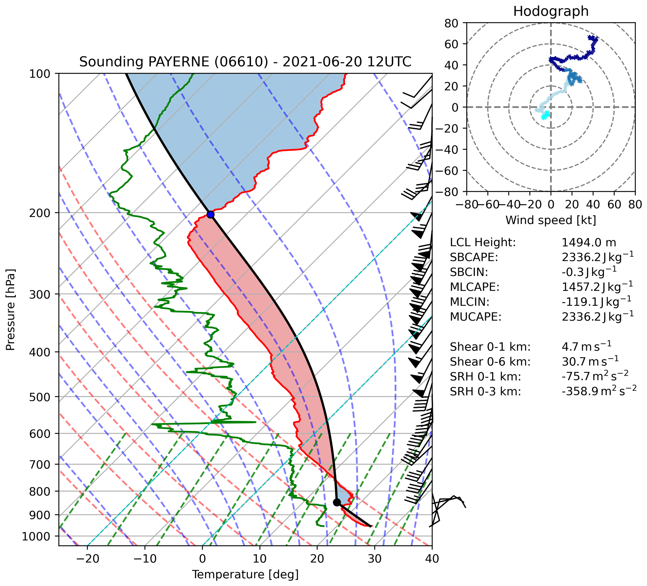
Figure 1Skew-T plot with hodograph analysis from the atmospheric radio sounding at the Payerne station (ID: 06610; 87 km WSW from the soccer field) on 20 June 2021 at 12:00 UTC, produced with the MetPy software (May et al., 2023). The temperature and dew point profiles are drawn in red and green. The shaded areas in red and blue mark the CAPE (convective available potential energy) and CIN (convective inhibition). The hodograph display shows four layers: 0–1 km (cyan), 1–3 km (light blue), 3–5 km (blue) and 5–10 km (dark blue).
In this study, we use aerial drone images collected on 20 June 2021. That day, the ingredients for long-living and well-organized severe thunderstorms (humid air, high instability and strong wind shear) were in place across Switzerland. An air mass with steep lapse rates was advected from the southwest above moist low-level air with mean mixing ratios around 12 g kg−1. Lapse rates above the capping inversion were close to dry adiabatic. The surface-based convective available potential energy (SBCAPE) was above 2000 J kg−1, and high wind shear of about 30 m s−1 in the 0–6 km layer was present at 12:00 UTC (Fig. 1). A supercell developed over the French Alps in the morning and moved through Switzerland within 5 h. The track of the supercell is shown in Fig. 2a and was generated based on the TRT (Thunderstorm Radar Tracking) algorithm (Feldmann et al., 2023; Hering et al., 2004). From the hodograph shown in Fig. 1, a storm motion vector of 234° at 13 m s−1 (according to Bunkers et al., 2000) and mean storm relative winds (0–6 km) of 71° at 9 m s−1 can be derived. This environment favored the development of classical right-moving supercells (Houze et al., 1993).
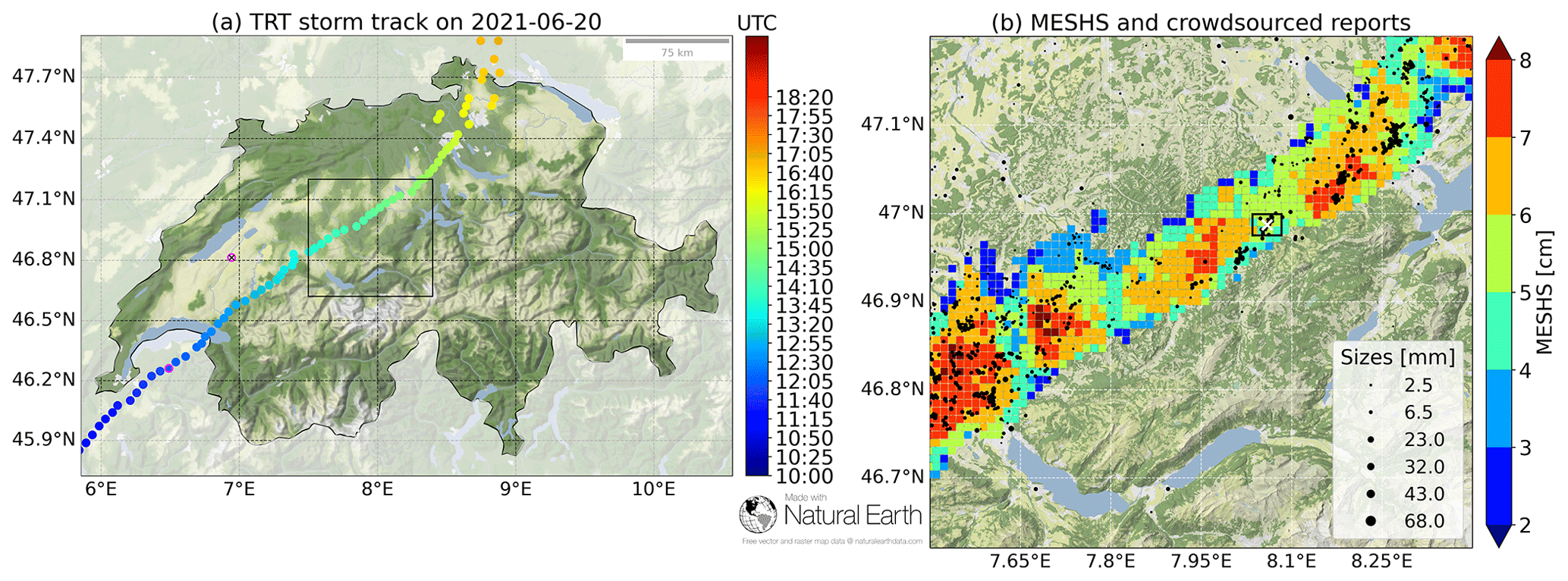
Figure 2Storm track (a) of the 20 June 2021 supercell with colored time information (5 min resolution of the scatter points) and the location of the atmospheric radio sounding (magenta open circle with black cross inside) shown in Fig. 1. The storm location at the sounding time (12:00 UTC) is marked with the same edge color (magenta). The black rectangle in panel (a) marks the zoom area for panel (b), where information about radar-derived MESHS (Maximum Expected Severe Hail Size) and crowdsourced hail size reports (black and different-sized circles) for six size categories with bin centers at 2.5, 6.5, 23, 32, 43 and 68 mm are given. The location of the soccer field, where the drone-based hail survey took place, is marked with a white cross. The black rectangle around the white cross in panel (b) marks the zoom area for the detailed map view in Fig. 3. Map tiles are by Stamen Design (https://stamen.com, last access: 3 March 2024) and Stadia Maps (https://stadiamaps.com, last access: 3 March 2024), under CC-BY-4.0. Map data from © OpenStreetMap contributors 2024. Distributed under the Open Data Commons Open Database License (ODbL) v1.0 and available from https://www.openstreetmap.org (last access: 3 March 2024).
The supercell produced a continuous hail swath from Lake Geneva to Zurich over a length of about 155 km, and the maximum hail size is estimated to have been above 60 mm. Both the maximum hail size and the hail swath are inferred from the MESHS products based on the Swiss operational radar network (Germann et al., 2022). Figure 2b illustrates the radar-derived MESHS signature from the supercell in the Napf region (central Switzerland), where the aerial images were collected on a soccer field (white cross) near Entlebuch (canton of Lucerne). For this location, MESHS indicates a maximum expected severe hail size of 63 mm, and on-site observations revealed maximum dimensions between 40 and 50 mm. In addition, data from four automatic hail sensors are available for the area within 1 km of the survey area. Surprisingly, the closest sensor (HS1; 300 m SSW from the soccer field) did not record any impact during the entire hail event. Therefore, we use the HSD data from the remaining three sensors in this analysis (Fig. 4). HS2 and HS4 are located NNE of the soccer field at distances of 770 and 1470 m, respectively, while HS3 is located SSW at a distance of 1150 m (Fig. 3).
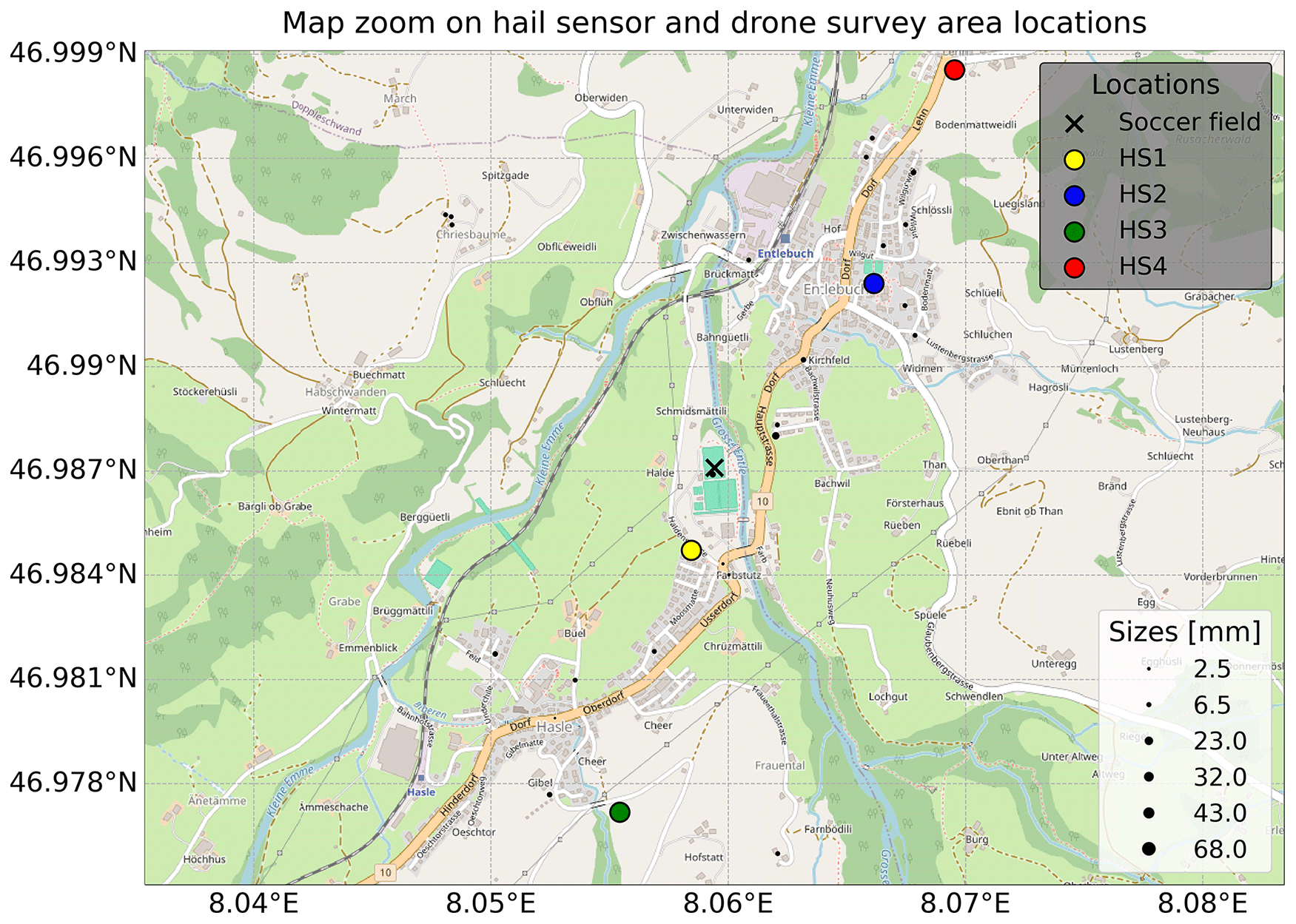
Figure 3The zoom area and detailed view for the black rectangle around the white cross in Fig. 2b. It shows the locations of the soccer field (roughly centered to the map view; black cross), the four nearest automatic hail sensors (HS1, HS2, HS3 and HS4) and the crowdsourced hail size data (black and different-sized circles). Map tiles are by Stamen Design (https://stamen.com) and Stadia Maps (https://stadiamaps.com), under CC-BY-4.0. Map data from © OpenStreetMap contributors 2024. Distributed under the Open Data Commons Open Database License (ODbL) v1.0 and available from https://www.openstreetmap.org.
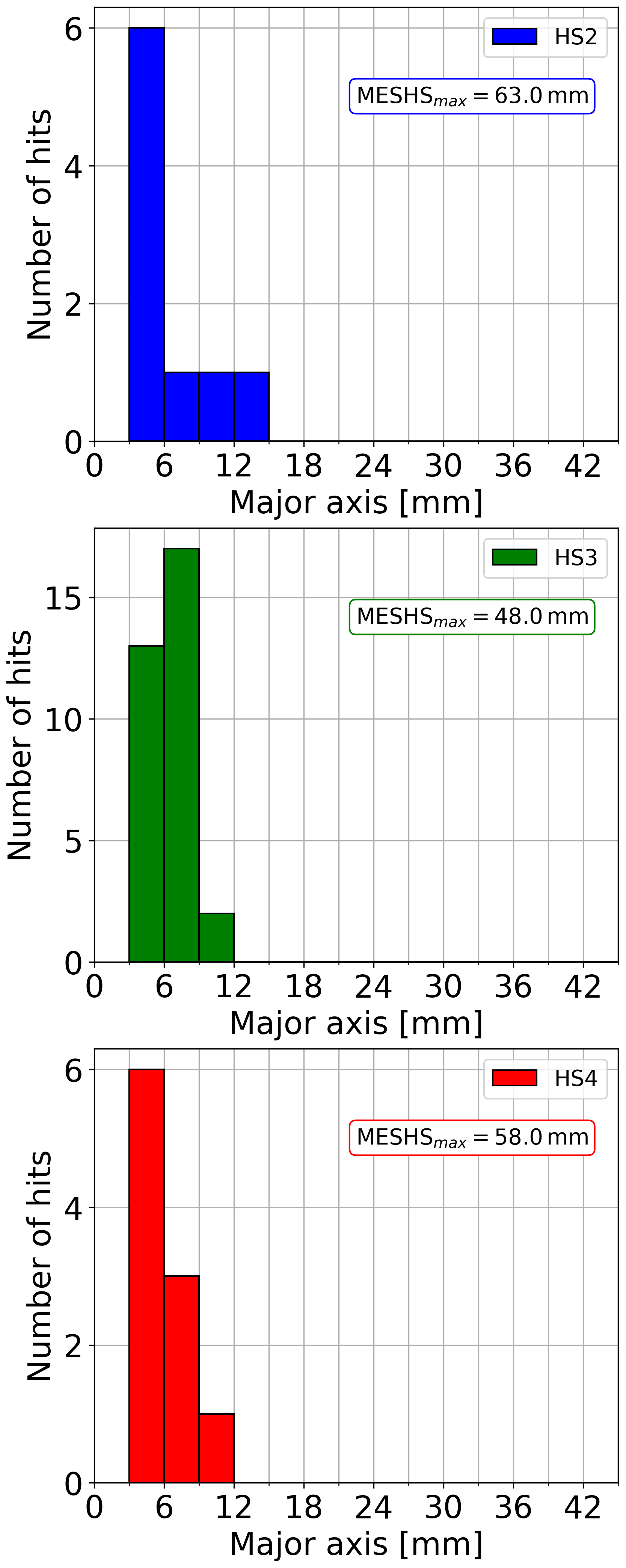
Figure 4Histograms of the recorded hail size distributions from the automatic hail sensors together with the daily maximum MESHS value at the sensor locations (see Fig. 3). The recorded hail durations for the sensors are about 3 min (HS2), 16 min (HS3) and 13 min (HS4). The color scheme follows the one from Fig. 3. The HS1 sensor did not record any hailstones and is thus omitted here.
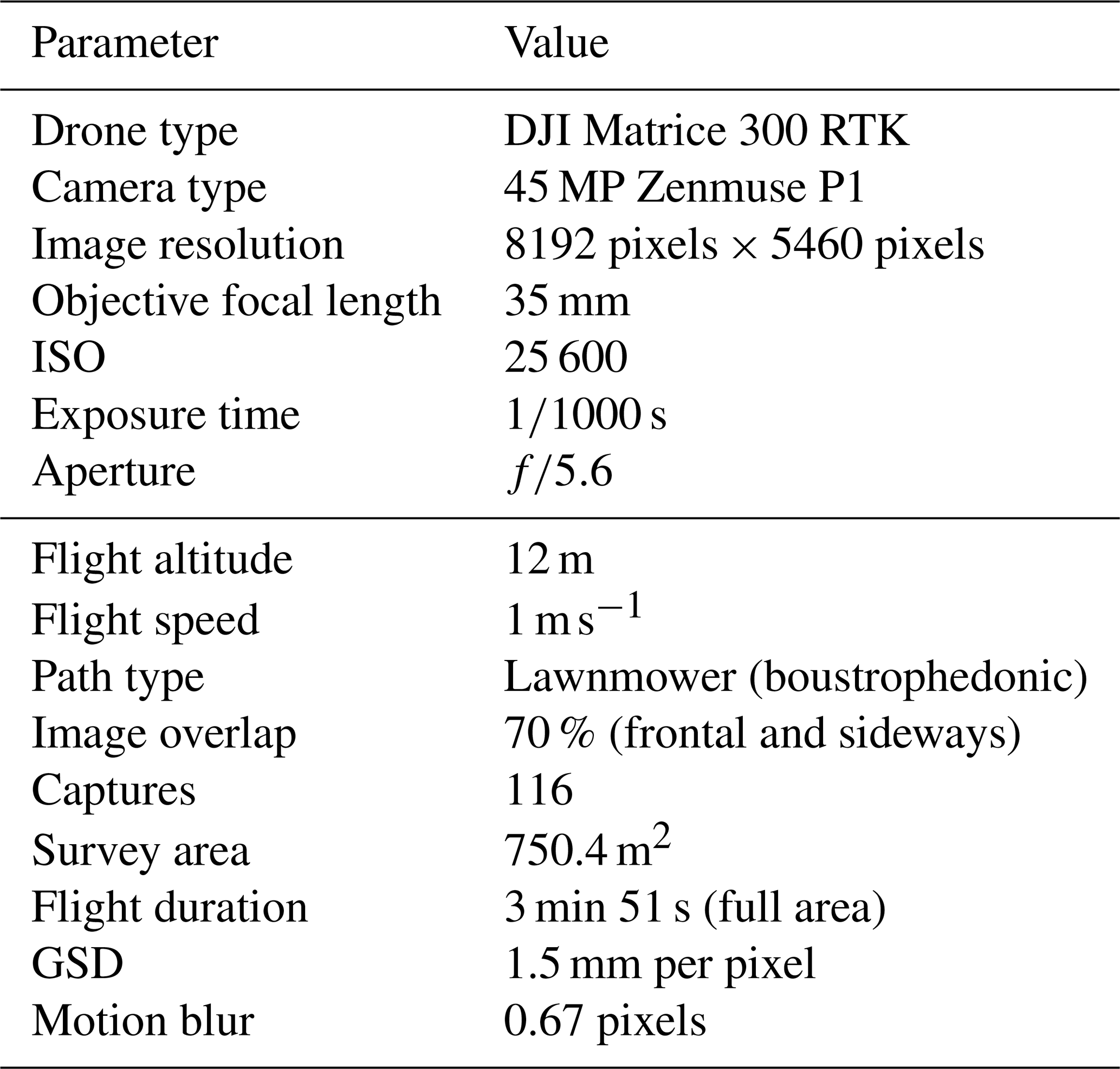
Soderholm et al. (2020) provided general recommendations to optimize the quality and further analysis of aerial drone images of hail: utilize uniform and contrasting backgrounds (cut or grazed turf grasses), ensure a high camera resolution for capturing smaller hailstones, minimize the melting of hailstones, avoid aerial surveys in areas with flowing water, and conduct surveys immediately after hail fall. Following those suggestions, we achieved a ground sampling distance (GSD) of 1.5 mm per pixel by flying at an altitude of 12 m with a 45-megapixel full-frame camera system. For the detailed flight and system characteristics, see also Table 1. Altogether it permitted us to classify hailstones down to a minimum size of 3–6 mm, which is a significant improvement compared to the minimum size of 20 mm from Soderholm et al. (2020). Here, the survey was performed on a soccer field with a visually homogeneous background and an excellent drainage of water. A main difference to the approach of Soderholm et al. (2020) is the technical setup to estimate the size of the identified hailstones. Instead of using an additional computer-vision-based method, here we only use the data from the deep learning algorithm to estimate the hail sizes and shapes. In addition, we present an approach to address the melting of hailstones on the ground; the melting rate is estimated by capturing the shrinking of the hailstones from images of successive drone flights. This allows for the approximation of the expected largest hail sizes at the start of the hail fall if the exact times of the storm passage and images are known.
Table 1Specifications of the drone, camera system and flight characteristics.
In Sect. 2, the methodology is presented, starting with the data collection procedure, a description of the equipment and details about the image data acquisition, followed by the post-processing, the hail detection with deep learning algorithms and the final retrieval of the hail size distribution. The resulting hail size distributions, performance of the model and melting rate estimation are described in Sect. 3. Further discussions to bring the findings to a broader context are presented in Sect. 4. Conclusions, ideas and suggestions for future analyses are given in Sect. 5.
In this study, we use a deep learning method to automatically detect individual hailstones in aerial images of hail. A subset of the images was annotated by a human expert and served as a training, validation and test data set. Furthermore, the test data set was annotated by two additional independent experts to objectively estimate the performance of the model. The method follows the HailPixel procedure described in Soderholm et al. (2020) that applies a two-stage approach, consisting of a machine learning technique to identify the center pixel of each hailstone in the image and a computer vision (CV) approach to detect the edges of the individual hailstones based on pixel lightness values. During a preliminary test in our study, the two-stage approach was compared to a one-stage method using solely a deep learning instance segmentation model based on Mask R-CNN to detect individual hailstones and estimate their sizes. With the two-stage approach, the edge detection did not work reliably for small hailstones in particular because the lightness gradient between these small hailstones and the background was insufficient. Here, we therefore focus on the one-stage approach.
2.1 Data collection and the experience from chasing hailstorms
A major challenge of drone-based hail photogrammetry is the collection of data. Hail-producing thunderstorms are highly localized phenomena, and falling hail melts quickly on the surface due to high (summer) air and soil temperature and sometimes strong rainfall following directly after the hail. Thus, to intercept a thunderstorm, the drone operators need to be on site before the arrival of the storm. Therefore, the availability of suitable nowcasting products and experienced interpretation are highly important. Aside from the meteorological challenges, the practical difficulties are even more pronounced. To obtain the best possible quality of aerial images, we focused on places where we were confident we would encounter freshly cut meadows. Public soccer fields turned out to be most promising target locations, which can be easily identified in interactive maps while being on the road, e.g., using https://map.geo.admin.ch/ (last access: 17 April 2024) (SwissGeoportal, 2023). In addition, major parts of the hail-prone areas were scouted in advance to determine potential locations to intersect a specific storm cell and familiarize with the local traffic routes.
During days with conditions favorable for supercells, the drone operators were already on standby in central Switzerland in the morning hours to be ready to head toward potential regions of thunderstorm occurrence. A valuable sources to identify such conditions and regions are the forecasts by ESTOFEX (European Storm Forecast Experiment; https://www.estofex.org/, last access: 18 April 2024). Our experience has shown that at least a level 2 on the ESTOFEX internal scale needs to be issued to have a realistic chance of intercepting a hail-producing cell. In general, the forecasts and evaluation of the synoptic situation across Europe provided on their website are highly valuable for the preparation process and determining whether meteorological conditions will be favorable the following day.
On the day of an event, different nowcasting and observational products were used. Most importantly, the operational radar images produced by MeteoSwiss served as a baseline to identify storms and nowcast the upcoming minutes to hours. The 3-dimensional reflectivity information is crucial to not only identifying the cell itself, but also further estimating the strength and exact location of a potential hail core. Within the operational radar products, POH and MESHS were used. Our experience has shown that in order to achieve promising results, POH needs to be 100 % and MESHS should reach stable values above 20 mm. Furthermore, satellite images and lightning information (e.g., lightning jumps; Schultz et al., 2009; Chronis et al., 2015; Nisi et al., 2020) help to focus on intensifying regions within the developing storm cells. Finally, real-time hail reports from the public can give a hint about the size of the hail that can be expected and to fine-tune the final decisions for a suitable location.
Following this strategy and using the tools mentioned, two drone-based hail photogrammetry surveys could be performed during 5 event days in 2021. In this study, we present an analysis of the data collected on 20 June 2021 to demonstrate the methodology. The data from the second available event cannot be taken into account because of low quality of the data. In particular, both the light conditions and the background (longer grass on the soccer field) were not optimal, and thus, the data unfortunately cannot be used for an in-depth analysis.
2.2 Drone operation and image processing
The aerial hail photogrammetry missions were performed with a DJI Matrice 300 RTK drone equipped with a Zenmuse P1 camera system that has a full-frame sensor (45-megapixel) stabilized by a three-axis gimbal and a focal length of 35 mm. The synchronization of the camera, the flight controller and the gimbal is done at a temporal resolution of microseconds and thus ensures a high accuracy of the image data. The drone was not operated with the RTK (real-time kinematic) feature enabled. This would require the installation of an RTK base station module. The advantage would be an increase in a positional accuracy of the drone from being on the order of a few decimeters to centimeters. Another potential option would be to use the NTRIP (Networked Transport of RTCM, Radio Technical Commission for Maritime Services, via Internet Protocol) standard. This protocol facilitates the transmission of correction data over the internet. It enables real-time positioning and precise navigation by delivering accurate correction data to GPS receivers.
As the first step, the individual images captured by the drone have to be combined into an orthomosaic. An orthomosaic is defined as a composite of multiple aerial (airborne or spaceborne) photos that are previously processed to remove inherent distortions caused by the geometrical properties of the lenses (airborne photos) and the curvature of the Earth (spaceborne satellite images). Thus, the processed individual pictures and the resulting composed orthomosaic are distortion-free and exhibit a true scale that allows for the estimation of the size of the objects in the photo. To generate an orthomosaic, an image overlap of between 70 % and 80 % is required (Guidi et al., 2020; Fawcett et al., 2019). Here, we use an image overlap of 70 % for both sides (frontal and sideways).
The flight pattern was programmed using the DJI Pilot 2 application. We defined a lawnmower (boustrophedonic) flight path without a crosshatch, with a flight altitude of 12 m above the ground (minimal possible altitude) and a flight speed of 1 m s−1. A low horizontal flight speed is necessary to reduce the motion blur (Bemis et al., 2014; Soderholm et al., 2020), which is within 1 image pixel (0.67 pixels) in our case and leads, in general, to small overestimations (≈1 mm) of the hail dimensions. The orthomosaic (or orthophoto) is generated using the open-source software OpenDroneMap (ODM; OpenDroneMap, 2020). This software can convert 2-dimensional images into classified point clouds, 3-dimensional textured models, georeferenced orthorectified imagery or georeferenced digital elevation models. ODM makes use of OpenSfM (mapillary, 2020), which is a structure-from-motion (SfM) library written in Python that depends on OpenCV (Bradski, 2000). The library can be used to reconstruct camera positions and 3-dimensional scenes based on multiple images (mapillary, 2023). Here, we make use of the basic modules of SfM: feature detection, feature matching and minimal solvers.
The orthophoto construction can be divided into the following main steps:
-
identification of matching points between the images
-
reconstruction of the camera perspective and the position of each image for the quality check and subsequent computation of the 3-dimensional coordinates of the matching points
-
derivation of a DEM (digital elevation model) using a reduced point cloud in 3-dimensional space
-
construction of the orthophoto by applying the DEM to the spatial projection of each image point.
The first flight started at 14:37:28 UTC, which is about 9.5 min after the start of the hail fall. Within 3 min 51 s, a total of 116 images were taken. Table 1 summarizes the detailed drone, camera system and flight characteristics of the hail photogrammetry mission. Although it is critical to get off the ground as soon as possible after the hail fall, environmental conditions like rain rate, wind and gust speed should be carefully monitored in order to stay within the permitted operation conditions of the drone model. The utilization of a relatively high ISO value, as outlined in Table 1, facilitates operational use even in challenging lighting conditions, maintaining low motion blur (0.67 pixels) at a constant flight speed of the drone. Furthermore, wind and gusts can affect the drone's stability, potentially leading to additional image blurring.
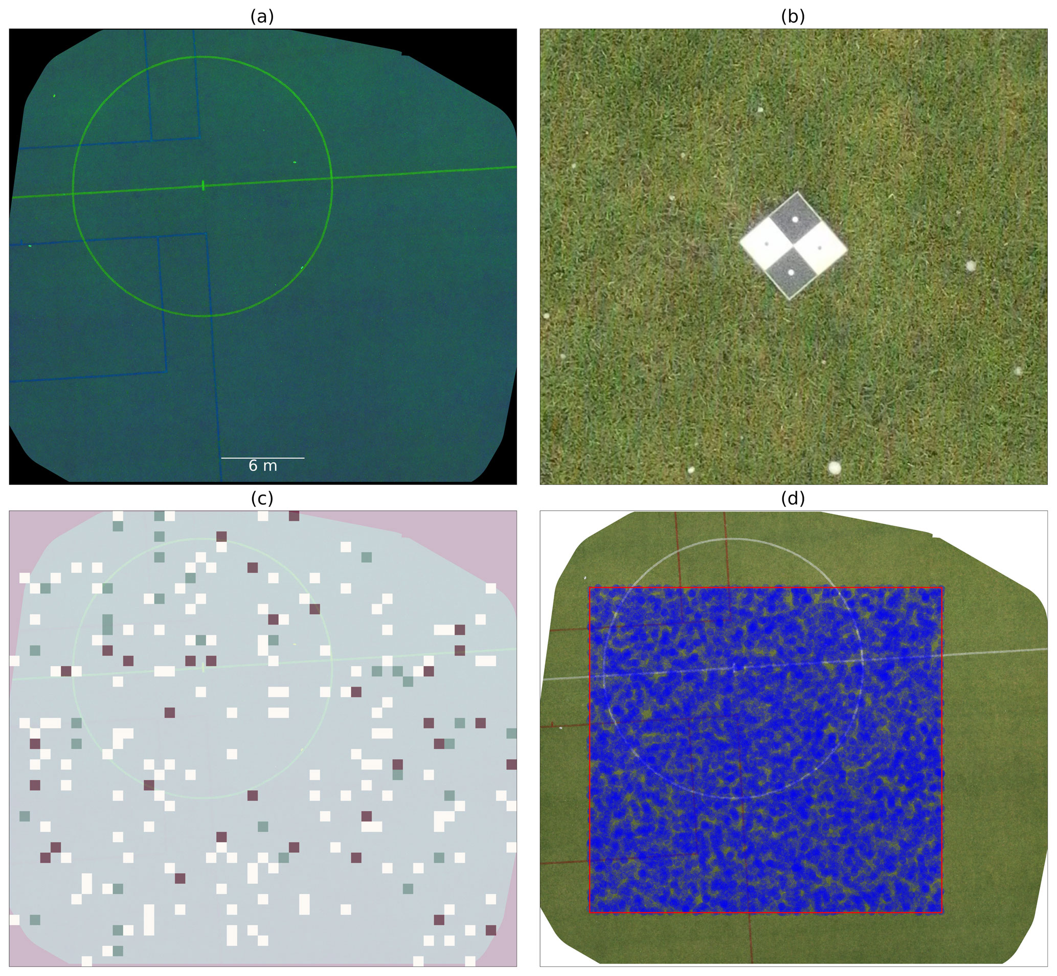
Figure 5In panel (a), the final orthophoto of the 20 June 2021 hail event is shown in the HSL (hue, saturation, lightness) color space. It is produced from 116 individual aerial drone images with the OpenDroneMap (ODM) software package. The radius of the soccer middle circle is 9.15 m. In panel (b), an image zoom from the orthophoto with an actual scale of 1 m (width) and 0.9 m (height) illustrates the hail appearance on the soccer field in conjunction with one of the reference objects (black and white circles of 10 mm diameters; black and white squares of 75 mm side lengths) to verify the ground sampling distance (GSD). In panel (c), the randomly selected distribution of training (light gray), validation (green) and test (dark red) image tiles (75 cm edge length) is displayed within the orthophoto. Panel (d) belongs to Sect. 3.2 and displays the same orthophoto in RGB (red, green and blue) color space overplotted by a 600 m2 area (red rectangle), where 10 000 circles of 0.2 m2 (virtual hail sensors; shaded blue) are randomly placed for statistical assessments.
A standard output of the ODM software is a quality report. The report gives a total of 14 916 215 reconstructed dense points and a mean GPS error of 0.34 m. The orthophoto covers an area of 750.4 m2 (see Fig. 5a) that shows an elevation change of 0.5 m. Multiple reference objects (see Fig. 5b) placed on the soccer field are used for an independent verification of the GSD. These reference objects were laminated printouts of geometric shapes in black and white – i.e., circles with a diameter of 10 mm and squares with side lengths of 75 mm. The white circles consist of 6 to 7 pixels within the orthophoto, which is equivalent to a diameter of 9–10.5 mm. Due to a slight overexposure in combination with the motion blur, the black circles on white background appeared approximately 1–2 pixels smaller.
2.3 Object detection and size estimation
Object detection is a computational method of automatically identifying and locating different objects or semantic classes (e.g., trees, bicycles and faces) within an image or a video. A comprehensive overview of the techniques and developments in object detection over the last 2 decades can be found in Zou et al. (2019). In recent years, many of the latest available neural network detection engines (e.g., AlexNet, VGG, GoogLeNet, ResNets, DenseNets) have been applied to object detection. For example, Mask R-CNN (He et al., 2020), as one of the state-of-the-art models for instance object segmentation, uses a residual neural network (ResNet) detection engine described in He et al. (2016) and is designed to simplify the training of deep neural networks.
We used the deep learning toolbox Detectron2 from Wu et al. (2019) as a starting point to train a model for automatic hail recognition. Its flexible design allows for switching between different tasks such as object detection, instance segmentation or panoptic segmentation. It provides built-in support for popular data sets like the MS COCO (Microsoft Common Objects in Context) described in Lin et al. (2014) and contains features from Faster/Mask R-CNN: ResNet in combination with a feature pyramid network (FPN), Convolution 4 (C4), as a single-scale feature map or a dilated convolution technique. Furthermore, Detectron2 provides ready-to-use baselines with pre-trained model weights. Here, we use one set of those pre-trained model weights to train a new model for hail detection only. Thus, we only have two classes – namely hail and the image background. The model is trained using data from a single event with grass in the background (soccer field). In order to generalize the model and apply it to additional data with different backgrounds (less homogeneous grass field, crop fields and concrete surface), the model should be retrained with additional data. However, not all backgrounds are suitable; for example, on a concrete surface (a public parking), the hail would melt much faster due to high solar irradiation that is likely prior to thunderstorms.
2.3.1 Image data preparation
The orthophoto exhibits a resolution of 24 500 pixels by 22 000 pixels, resulting in a total of 5.39×108 pixels and disk space used of about 2 GB. The ODM software provides different output formats for the orthophoto. Here we use a PNG (Portable Network Graphics) format for the subsequent analysis. As shown in Fig. 5a, the orthophoto does not cover the entire image size, reducing the total number of analyzed image pixels to about 5×108 pixels. Thus, given the GSD of 1.5 mm per pixel, the entire image covers an area of 750.4 m2.
The original orthophoto is divided into smaller image tiles to save computational resources during the training of the model. A reasonable compromise is a size of 500×500 pixels for each tile. We use a randomly selected 10 % of the tiles as reference data (216 tiles). These reference data are further divided into 70 % for training (150 tiles) and 15 % for the validation (33 tiles) and test data (33 tiles). These data sets are visually analyzed by expert A, and all hailstones are annotated using the Computer Vision Annotation Tool (CVAT; Sekachev et al., 2020). The resulting annotation files are based on JSON (JavaScript Object Notation) and store information about each image tile. This includes the path, width, height, annotation identifiers of the hailstones and the polygon coordinates defining their instance segmentation masks. Overall, the training data set contains 937, the validation data set 249 and the test data set 215 hailstone annotations. To account for differences in the visually determined annotations, two more human experts (B and C) annotated the test data set independently. Thus, the test data set annotated by experts B and C is used as an independent data source to assess the model prediction performance.
2.3.2 Hail detection and size estimation – training, validation and testing
The main concept behind deep learning models is to split the reference data set into a training, a validation and a test data set. The training data set is used to estimate the model parameters. Within the training procedure, a validation data set is used to prevent overfitting and to assess the evolution of performance indicators during the entire training run in steps of 100 iterations. Furthermore, an independent test data set is necessary that serves as a truth against which the model results (applied to data not contained in the reference data set) and thus the model performance can be assessed. As mentioned before, we use independent test data sets where hail is visually detected by three experts (see Fig. 9).
An NVIDIA GeForce RTX 3060 Ti was used to efficiently train the Mask R-CNN model on the training data set. This GPU model has 4864 Compute Unified Device Architecture (CUDA) cores and a total of 8 GB GDDR6 RAM available. A default configuration of Detectron2 is used to estimate a first set for the hyper-parameter tuning. We started with a base model that was pre-trained using the MS COCO data set based on ResNet and FPN. The MS COCO data set consists of about 2×10⁵ annotated images with a total of 80 different object classes, and it is thus an ideal starting point for training deep learning models to recognize, label and describe objects.
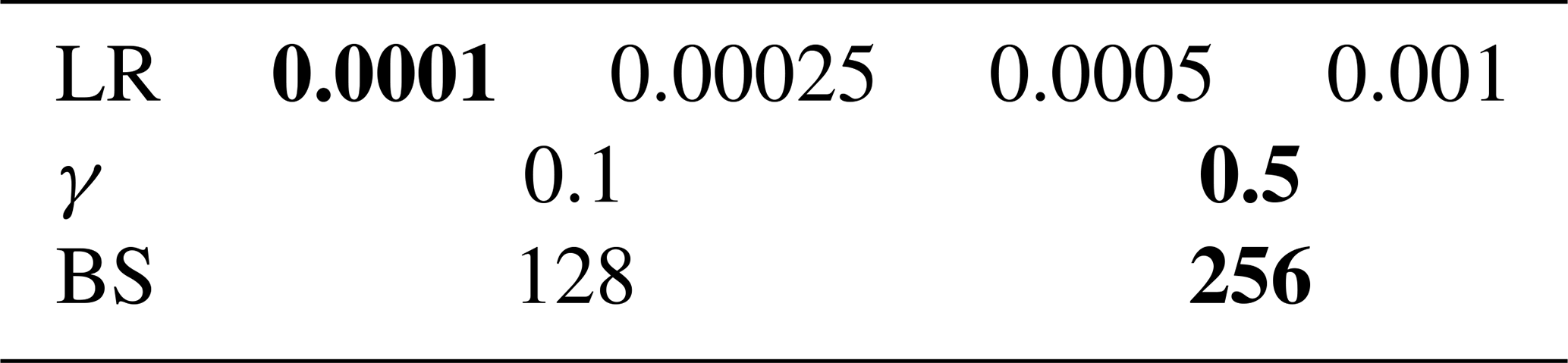
To assess various hyper-parameter combinations (see Table 2), 16 different training runs (run 0 to run 15) were performed. Here, we only vary the three hyper-parameter learning rate, the gamma value and the batch size to show a proof of concept for automatic hail detection. For detailed information about the concept and additional available parameters, we refer to Schmidhuber (2015) and Wu et al. (2023). These training runs were performed for each of the 150 image tiles in the training data set. Using two images per batch with 1 GPU, a total of 75 batches are needed, and this represents one epoch time (i.e., one iteration through all available image tiles). We then performed 40 epoch times, resulting in a total of 3000 iterations.
Table 2Range tested for the three hyper-parameters: learning rate (LR), γ value (γ) and batch size (BS) per image. The hyper-parameter combination of the model with the lowest validation loss after 3000 iterations is highlighted in bold.
During an individual training run, the validation is done every 100 iterations. Thus, for one training run with a total of 3000 iterations, we obtain a temporal evolution of the scores along 30 points. Figure 6 shows the progress of the total loss and the validation loss for all 16 training runs performed. The bold lines depict the run exhibiting the lowest validation loss after 40 epoch times. To chose the best model, we performed a more detailed evaluation of the model runs by means of commonly used metrics in object detection.
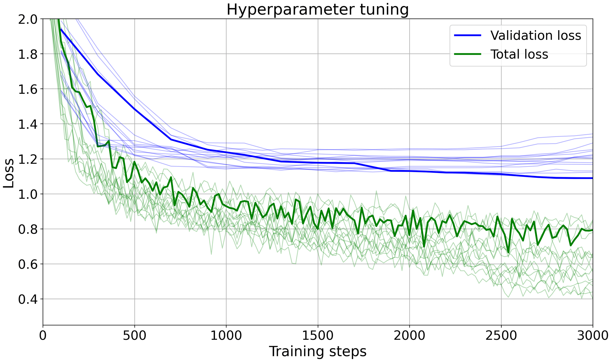
Figure 6Line plots of the evolution of validation loss and total loss along the training iteration steps for the 16 deep learning model runs with different combinations of hyper-parameters shown in Table 2. The thick lines depict the training run 3, used for prediction of hail pixels.
To assess the performance of a model, diverse metrics are available. A single score (i.e., performance metric) provides the model performance from a certain perspective and thus different scores should be taken into account. A score compares the predicted result with the truth based on a confusion matrix (Wilks, 2011). In image classification, the predicted results of an individual feature (i.e., hailstone in our case) usually do not exactly match the truth (the same hailstone in the test data set), but the area of overlap can vary. We therefore use the ratio of the intersection over union (IoU). The IoU ratio is defined as the ratio between the overlap and the union of the bounding box around the features of the predicted result and the truth. In our case, we use the instance segmentation mask (i.e., the one segmentation mask for each individual feature) instead of the bounding box to compute the IoU ratio. The IoU ranges from 0 to 1, and a ratio of 0.5 is used to define a correct prediction and thus interpreted as a true positive (TP) result. A predicted result with an IoU lower than 0.5 is thus a false positive (FP), and if no results are predicted for an existing feature in the truth, it is depicted as a false negative (FN). Following the standard COCO evaluation procedure, the set of IoU ratios for a TP ranges from 0.5 to 0.95 in increments of 0.05.
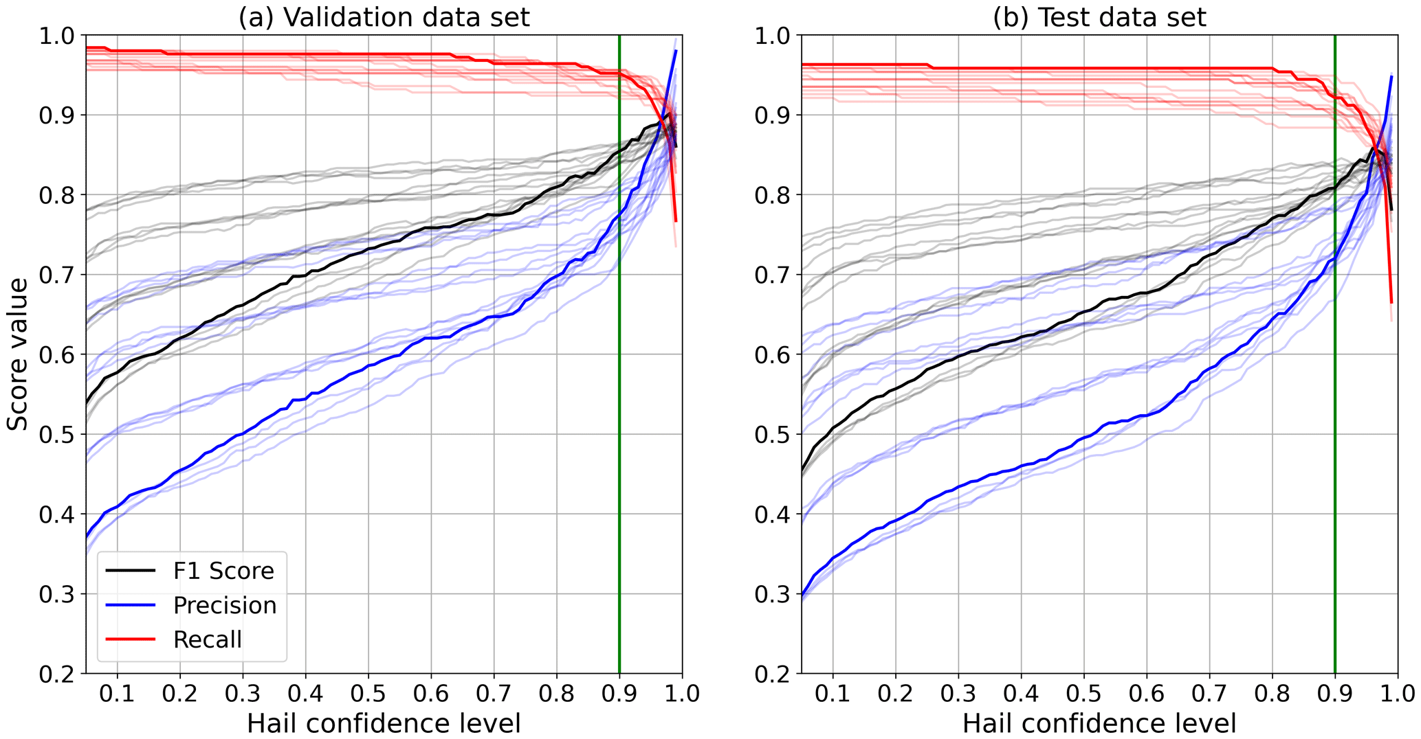
Figure 7Spaghetti plots of precision (blue), recall (red) and F1 scores (black) against the hail confidence level for all 16 deep learning model runs applied to the validation data (a) and the test data (b). The thick lines depict training run 3, used for the prediction of hail pixels. The vertical green line marks the 90 % hail confidence value that has been chosen as the lower limit for the object classification.
In machine learning, precision and recall (Eqs. 1 and 2) are commonly used (Powers, 2020). Precision depicts the number of true positive results divided by the total number of positive results. Recall refers to all true positive results divided by the number of all samples that should have been classified (i.e., as visually identified by the experts in the test data set in our case). Precision and recall can be combined in the F1 score in Eq. (3) (Van Rijsbergen, 1979; Goutte and Gaussier, 2005). The F1 score results in values from 0 to 1, where 0 indicates extremely poor performance and 1 refers to a perfect performance of the model.
Here, we prioritize the precision and aim at a large portion of correct detection (TP) of hailstones and low false positive results (i.e., hail detected by the model but not present in the test data set). Thus, as a trade-off, some hailstones are missed (FN), and the selected threshold does not exactly correspond to the optimal F1 score. A reasonable compromise between precision and recall is found at a hail confidence threshold of 0.9 for run 3 (see Fig. 7), where F1 is close to 0.8 (0.85), when evaluating against the test (validation) data set. The appearance of four groups in the two plots of Fig. 7 is due to the four different learning rate values tested (Table 2).
Of the 16 different training runs, run 3 was chosen as the model to apply to the orthophoto for automatic hail detection. Thus, run 3 was applied to all available image tiles (2156), and the instance segmentation masks of each detected hail object were saved in separate Python structures linked to the individual images. In total, 18 209 objects were classified as hail, but two of them were discarded as they were in the very small bin size (between 1 and 2 mm). A visual evaluation of the largest objects revealed some leaves that were incorrectly classified as hail and therefore manually removed to guarantee a correct representation of the largest hail size bins in the distribution.
In the validation data set with 249 annotated hailstones, 237 are TP and 12 are FN, resulting in a false negative rate, , of 4.8 %. For the test data set with 215 hailstones, 198 are TP and 17 FN, which yields an FNR of 7.9 %. An additional performance metric used to describe the accuracy of a model is the mean average precision (mAP). In short, mAP depicts the average relationship between precision and recall across all IoU classes (from 0.5 to 0.95). The mAP for the validation (test) data set results in 0.53 (0.50) for the 90 % hail confidence threshold. In addition, Fig. 8 shows the number distribution of the IoU for all true positive matches (hail confidence level Ci≥0.9) within the validation (blue bars) and the test (green bars) data set. The majority of the IoUs lie above 0.7, indicating a good match between the predicted hailstones and the truth. For the test data set, a bi-modal distribution is found, with peaks around 0.76 and 0.86.
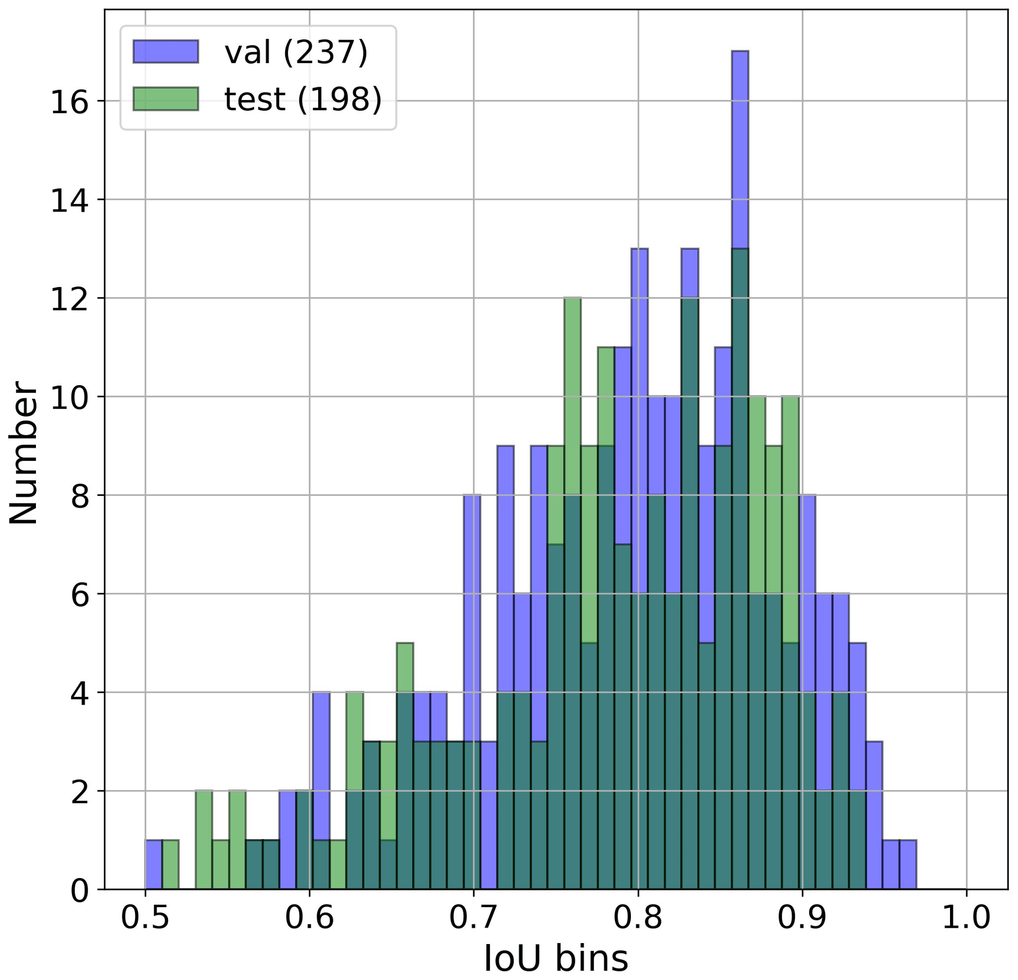
Figure 8Histograms of IoU (intersection over union) ratios between the prediction masks of model run 3 (hail confidence Ci≥0.9) and the validation data set (blue) and the test data set (green). The histogram area of the overlap between green and blue bars is shown in dark green. Only true positive (TP) matches, defined as IoU > 0.5, are shown. In the validation (test) data set, 237 (198) hailstones are classified as TP.
As mentioned in the beginning, the test data set is visually classified by three independent human experts. This allows for the assessment of the uncertainty in the test data set resulting from the visual detection of the hailstones. The hail size (in terms of major-axis length) is derived from the annotated polygons in the test data set and the model output. The resulting HSDs with a bin size of 3 mm are presented in Fig. 9. It shows that expert B and expert C have a peak number of hailstones within the 6–9 mm major-axis hail size bins. The median value of these experts' assessments is 10.5 mm. In comparison, the highest number of hailstones and the median value of expert A are found in the next higher bin class. Overall, the discrepancies are largest for the smallest size bin (3–6 mm). This indicates that the orthophoto resolution is a limiting factor for the reliable identification of such small hailstones by visual classification, as this size class suffers due to low brightness and a translucent background (see also Sects. 3 and 4).
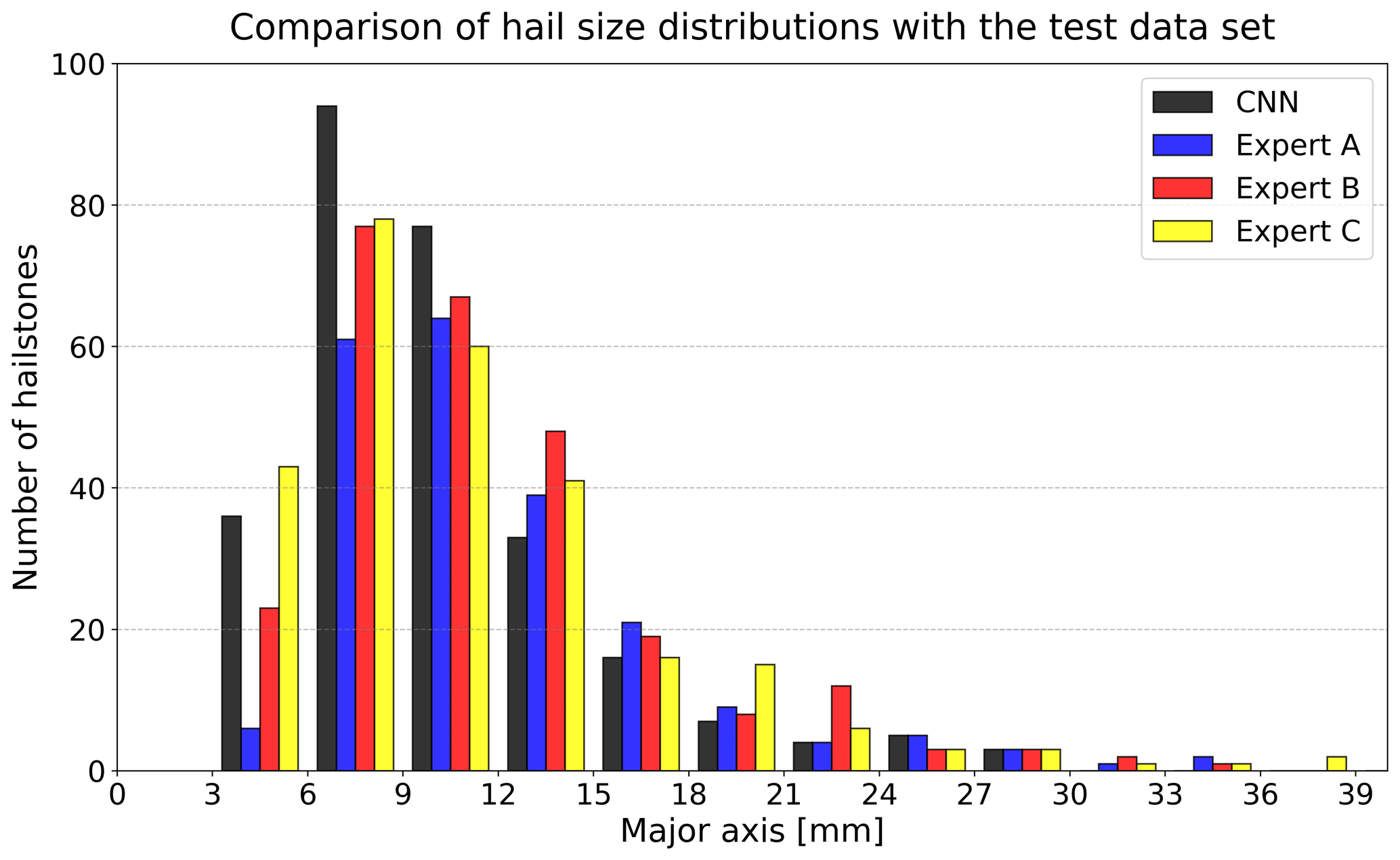
Figure 9Comparison of four hail size distributions from the test data set derived from manual annotations by three experts (A: blue; B: red; C: yellow) and the prediction of the Mask R-CNN model (black). The total numbers of identified hailstones by the experts are 215 (A), 263 (B) and 269 (C). The CNN (convolutional neural network) predicted 275 hail segmentation masks.
In this section, we first present the resulting hail size distribution from the first flight performed on 20 June 2021. We compare the HSD retrieved from the photogrammetric approach presented above to the HSD retrieved by four nearby hail sensors (Sect. 3.1). Subsequently, we assess the sampling error of hail sensors covering an observational area of 0.2 m2 with a sub-sample of data retrieved from the drone observation of an area of 600 m2 (Sect. 3.2). In Sect. 3.3, we estimate the melting rates of hail on the ground based on the evolution of the HSD from all five successive flights.
3.1 Estimation of the hail size distribution
The HSD estimated from the aerial photogrammetric data is shown in Fig. 10. The distribution contains a total of 18 207 hailstones, and the size refers to the major axis, determined by the machine learning algorithm. Of those, 45 hailstones are larger than 30 mm, with the largest being 39 mm. The mode of the distribution lies in the 6–9 mm bin. Only a few hailstones are larger than 21 mm. The closest automatic hail sensor (HS2) recorded nine impacts within 3 min and a maximum hail dimension of 14 mm (Fig. 4). The duration of the event at the location of the drone survey was ∼9.5 min. Estimated duration based on the neighboring hail sensors ranges from 3 min for HS2 to 13 min for HS4 and 16 min for HS3. The upscaled density of hailstones detected by the HS2 sensor is 45 hailstones per m2, compared to 24 hailstones per m2 on average as retrieved from the drone data. This might be related to the inherent spatial and temporal variability in hail, as the automatic hail sensor is located at a distance of about 770 m downstream of the area observed by the drone. In addition, the sensor detects the hail during the event, whereas the drone data are collected after the hail stops to avoid the drone being damaged. Therefore, the drone data are affected by melting processes and thus tend to underestimate the hail size and the number of small hailstones in particular. Furthermore, small hailstones might not be detected within the drone data as they might partially be obscured by the grass and by low differences in the lightness values compared to the background. Lightness values come from the HSL (hue, saturation and lightness) color space and range from 0 to 255. Mean lightness values (orange line in Fig. 10) of the 3–6 mm hailstones drop below 180, which is similar to the background. Size estimation based on edge detection methods that use lightness values alone, such as that proposed in Soderholm et al. (2020), therefore cannot be applied.
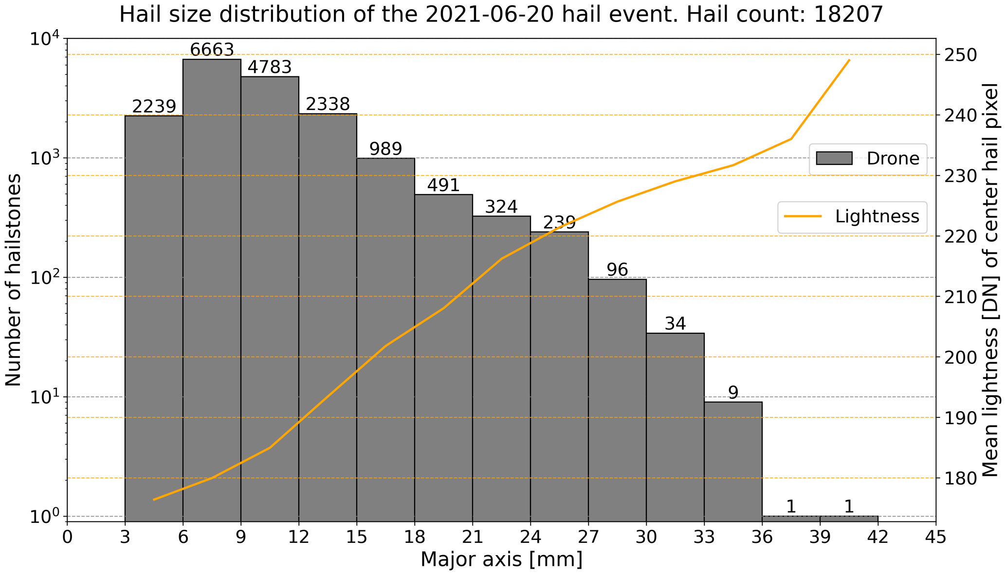
Figure 10Logarithmic view of the time-integrated hail size distribution of the 20 June 2021 event captured by the drone between 14:37:28 and 14:41:19 UTC. The total number of detected hailstones per each bin is shown by the number above each bar. Altogether, 18 207 hailstones were identified. The orange line represents the mean lightness value as digital number (DN) of all derived center hail pixels in the HSL (hue, saturation and lightness) color space for each hail size bin.
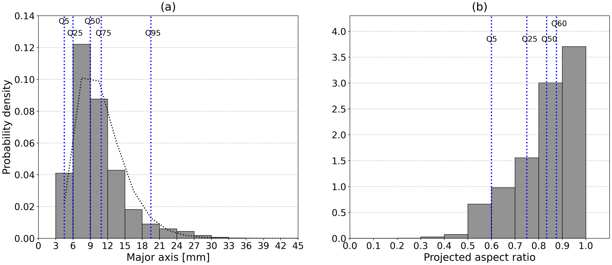
Figure 11Probability density distributions of the hail major axis (a) and the projected aspect ratio (b) between minor- and major-axis lengths in the image plane. The vertical dashed blue lines indicate the position of the particular quantiles with respect to the major axis (Q5, Q25, Q50, Q75 and Q95) and projected aspect ratio (Q5, Q25, Q50 and Q60). The HSD in panel (a) is additionally fitted against a gamma distribution (dotted black line).
The same drone-based HSD as in Fig. 10 is shown again as a function of the probability density in Fig. 11a. A gamma probability distribution function (PDF) is used to approximate the empirical HSD. The gamma PDF is most suitable for characterizing the distribution of the hailstone major axis, as shown by Ziegler et al. (1983) or Fraile et al. (1992). Overall, the gamma PDF closely follows the empirical distribution retrieved from the drone data, with a median of 9 mm and a slight underestimation of the peak (see Fig. 11a). The projected hail aspect ratios indicate that the majority of hailstones are rather spherical, with axis ratios greater than 0.9 (Fig. 11b). Furthermore, 75 % of the hailstones have projected aspect ratios higher than 0.75.
3.2 Sampling error within automatic hail sensor data with respect to drone-based data
In this section, we estimate the probability that a randomly placed hail sensor is hit by a hailstone of a certain size. A total of 10 000 virtual hail sensors with a size of 0.2 m2 were distributed across an area of 600 m2 within the orthophoto (blue circles in Fig. 5d). For each virtual sensor, the HSD was derived, and the individual kernel density estimates (KDEs; gray lines) are shown in Fig. 12a. The KDE was obtained from 7817 virtual sensor areas. The remaining 2183 sensors did not have enough virtual impact to estimate the kernel density. The distribution from the entire 600 m2 area is shown in black, and the respective quantiles (Q25, Q50 and Q75) from all the virtual sensors are shown in blue, red and green.
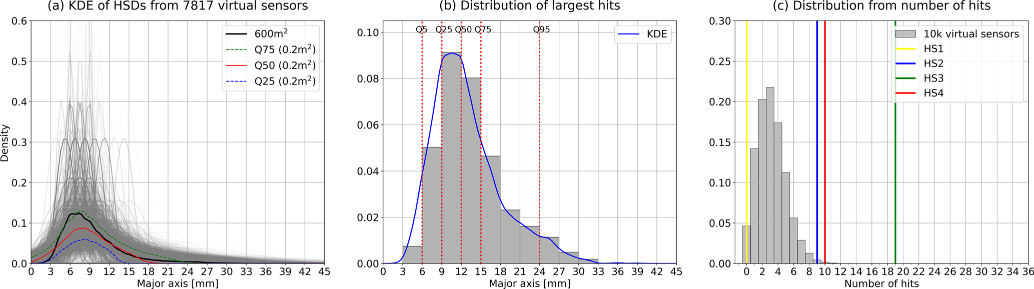
Figure 12Kernel density estimation (KDE) of HSDs (hail size distributions) from simulated hail sensors at random locations (a) on an area of 600 m2 (red rectangle in Fig. 5d). From the 10 000 virtual HSDs, 7817 can be represented by a KDE (gray curves), whereas the others do not have enough impacts. The quantiles of the sorted HSDs are shown as dashed blue (Q25), dashed green (Q75) and solid red (Q50) curves. For comparison, the KDE as derived from the whole 600 m2 area is overplotted in black. In the center (b), the KDE distribution for the aggregation of the largest hailstone impact on each virtual sensor is shown. Quantile markers (Q5, Q25, Q50, Q75 and Q95) are drawn on top of panel (b) in vertical dashed red lines. On the right side (c), the probability density for the total impacts on each virtual sensor is shown as a gray histogram, together with the registered number of impacts of the four closest automatic hail sensors HS1 (cyan line), HS2 (blue line), HS3 (green line) and HS4 (red line).
Of all virtual hail sensors, only 45 hailstones with a size larger than 30 mm are observed, and thus only 0.3 % (34 out of 10 000) of the virtual sensors exhibit an impact of such large hail. Furthermore, 9.9 % (988) of the virtual sensors observe impacts from hail with a size larger than 20 mm and 65.8 % (6576) from hail with a size larger than 10 mm. Moreover, the probability that a sensor records no impact at all is 4.7 %. Figure 12b shows the distribution of the largest hailstones, as observed by each virtual sensor. The median value reaches 12 mm, and the 95th percentile (Q95) corresponds to 24 mm. Figure 12c shows the distribution of the number of hailstones observed by all virtual hail sensors and compares it with the number of observed hailstones by the four physical hail sensors. The locations of those sensors are shown in the map in Fig. 3. All physical hail sensors were within the hail path (100 % POH region at a 1×1 km resolution).
The highest probability (22 %; see the peak of the histogram in Fig. 12c) is given by three impacts on a virtual sensor. The probability of 0 impacts (e.g., HS1; cyan line) is 4.7 %, and the probability of 9 or 10 impacts (HS2 and HS4; blue and red lines, respectively) is lower than 2 %. The third sensor (HS3) recorded 32 impacts, which is higher than the maximum number of impacts (12) recorded by all individual virtual sensors. This indicates that the spatial variability might play an important role and/or that the limitation of the drone data regarding the melting process prior to the flight might affect the estimation.
3.3 Melting on the ground and implications for hail size distribution estimations
A major limitation of drone aerial photogrammetry is its timing with respect to impact. Hail from the beginning of the event is thus already affected by melting and decreases in size until the drone observation can take place. In this section, we quantify the impact of melting by comparing the data from five successive drone flights. This allows for the estimation of the temporal evolution of the HSD. Figure 13 illustrates the shape evolution of two prominent hailstones during the melting process. Due to slight deviations in the derived orthophotos from varying GPS errors (0.21 to 0.5 m) and the melting process itself, the location of the center hail pixel changes and leads to misalignments for an individual hailstone across the successive flights. Therefore, we only use a subset of the orthophotos and select the area within the soccer middle circle, which can be unambiguously identified. The GSD between the flights stays constant at 1.5 mm per pixel, as confirmed by the reference objects.
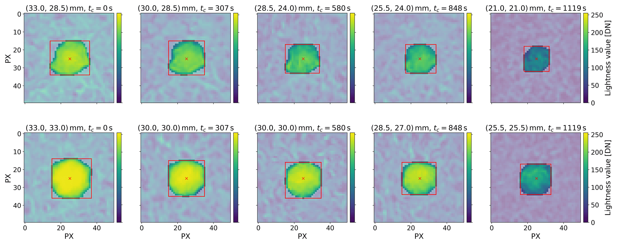
Figure 13Two examples of hailstone size and mask shape development during the captured melting process on the ground. From left to right, the sequential lightness images of two hailstones (row 1 and 2) extracted from the five orthophotos (soccer middle circle) are shown. In the images the Mask R-CNN segmentation masks are emphasized together with the major- and minor-axis lengths indicated by the minimal bounding boxes. The actual sizes (width and height) are given in the titles as well as the time tc since first capture. During the 1119 s these hailstones shrink about 12 mm (upper row) and 7.5 mm (lower row) in their major-axis length.
The area of the soccer middle circle (263 m2) is well defined, with a radius of 9.15 m. Within 18.65 min, the time between the first and the last drone flight, the number of hailstones decreased by 64 % (see Table 3). The evolution of the KDE retrieved from all individual drone flights is shown in Fig. 14. A clear shift in the peak and the upper tail toward smaller major-axis lengths can be observed. The shift in the plateaus on the upper tail indicates melting rates on the order of 0.5 mm min−1.
Table 3Time slots, in UTC, when the aerial pictures of the soccer middle circle (263 m2) were captured for the five drone mapping flights. From the first to the last orthophoto, 1119 s (18 min, 39 s) elapsed.
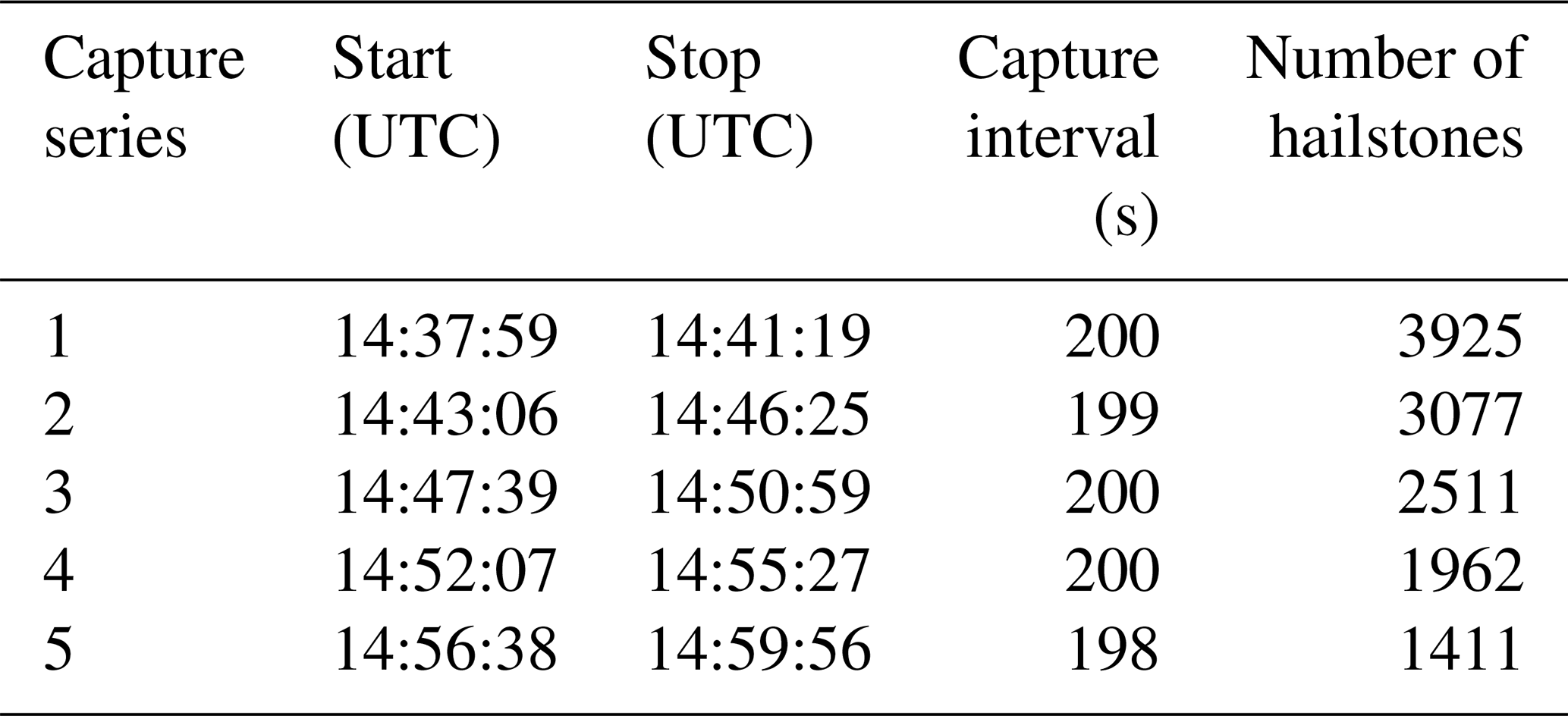
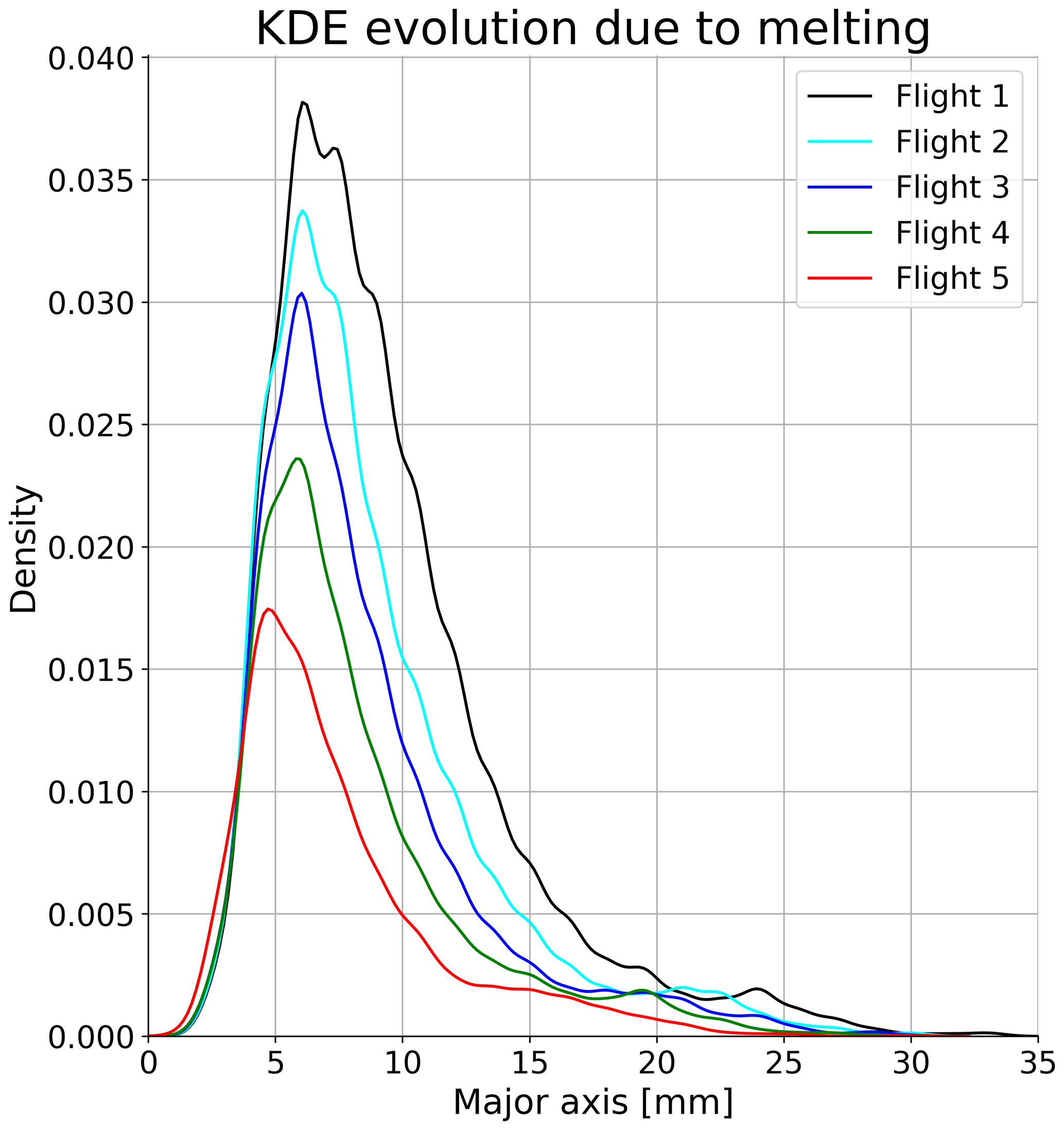
Figure 14Kernel density estimation (KDE) of the degrading hail size distributions due to melting processes on the ground. The initial hail sample size is 3925. The orthophoto area for the melting analysis is restricted to the soccer middle circle to ensure a correct comparison between the different generated orthophotos (Flight 1–5). In total, five drone-based hail photogrammetry surveys were carried out to capture the temporal data analysis. All the relevant time frames are listed in Table 3.
Using this melting rate estimate together with the time difference between the start of the hailstorm and the first drone flight, we infer that the initial size of the largest captured hailstone (39 mm) was 44 mm. Most crowdsourced reports in the vicinity of the soccer field indicated sizes from 30 to 50 mm, and the MESHS estimate was 63 mm (see Fig. 2b). On-site measurements by storm chasers during the hail event revealed maximum hail dimensions between 40 and 50 mm as well.
A major challenge for drone-based photogrammetry of hail is related to the appearance of the hail within an orthophoto. The hailstones need to show distinct differences from the background. This is not always the case as hail is formed by a combination of dry and wet growth processes, which can lead to varying densities and appearances of the ice. Dry growth produces high densities of microscopic air bubbles that scatter light, while wet growth causes liquid to soak into gaps and accretes on top of existing outer ice to form clearer ice. Hailstones can grow in both regimes, leading to alternating layers of cloudy and clear ice (Allen et al., 2020; Kumjian and Lombardo, 2020; Brook et al., 2021). The effectiveness of various methods used to detect hailstones is influenced, in part, by the transparency of the ice.
First, a simple computer vision approach (without neural networks) was tested to extract the segmentation hail masks. The approach was based on lightness thresholds, morphological transformations and watershed algorithms (Najman and Schmitt, 1994) for image segmentation with OpenCV (Bradski, 2000). The success and reliability of this approach highly depended on the visual appearance of the hailstones. For larger hail exhibiting distinct lightness difference compared to the background, this approach was promising. But for small hailstones exhibiting lower lightness values (Fig. 10), the CV-based edge detection (see Sects. 1 and 5) failed. For hail events with different characteristics (e.g., with a high number of small hailstones that aggregate in clusters on the ground), watershed algorithms could retrieve more reliable information.
Second, a deep learning model (Mask R-CNN) was tested. We used one single hail class to train the model. Additional hail size classes might improve the hail predictions and mask shapes. In particular, a distinction between damaging and non-damaging hail with a threshold of 20 mm could be worth testing. Furthermore, additional testing of the hyper-parameters might increase the performance, but this was outside the scope of this study.
Another technical challenge arises from splitting the orthophoto into smaller image tiles, which can result in truncated hailstones. This can be overcome by producing tiles which overlap by the maximum length of the largest observed hailstone, as implemented by Soderholm et al. (2020). However, in our case, large hail was sparse, and, as the image tiles cover large areas (500×500 pixels), it is safe to assume that the number of truncated hailstones is very low. Other sources of errors such as false positive detections or missed hailstones likely play a more important role.
Hailstones usually have an oblate spheroid shape, with mean axis ratios close to 0.8, though they can sometimes have large protuberances (Knight, 1986), and the probability for nonspherical shapes rises with increasing maximum dimension (Shedd et al., 2021). As a consequence, the hail aspect ratio decreases for larger sizes, as shown in the various studied data sets (Knight, 1986; Soderholm et al., 2020; Shedd et al., 2021). Figure 6 in Shedd et al. (2021) shows the comparison of their recent results regarding the evolution of aspect ratios with maximum hail sizes from manually measured hailstones to the results of Knight (1986). The slopes of the decreasing aspect ratios are comparable, but the absolute values tend to be lower in the hail data set of Shedd et al. (2021), reflecting possible effects of melting before the measurements were taken. Likewise, with hailpads, the shape factor in the image plane can be determined with the aerial drone-based hail photogrammetry, but the estimated aspect ratios (Fig. 11b) may differ from in situ measurements as published in Knight (1986) and Shedd et al. (2021). The hail images show only the projected maximum and minimum axes, which may differ from the ratios of true stone axis.
Another limitation of drone-based photogrammetry is that melting already affects the hail before the data can be collected. The effect of melting hail in the air was studied by Kumjian and Ryzhkov (2008) using polarimetric radar measurements, and numerical model investigations were performed by Fraile et al. (2003). Other studies by Rasmussen and Pruppacher (1982) and Rasmussen and Heymsfield (1987) have explored the melting of spherical ice particles falling at terminal velocity. They found that the melting rate depends on the initial size of the spheres and the surroundings, including temperature, humidity, turbulence and how meltwater is shed. The hailstones in our case are already on the ground, so they experience different environmental conditions compared to when they are falling through the atmosphere. We have not measured these specific conditions for each hailstone, so we cannot make any conclusions about how the melting rate relates to their initial size.
To our knowledge, there are no studies that analyze the melting of a large sample size of hail on the ground. Here, we provide a first estimate of the melting process of hail on the ground. More in-depth investigations would be needed to retrieve more accurate results – maybe also in relation to initial hail sizes and environmental conditions like the ground temperature and occurrence of rain before, during and after the hail event.
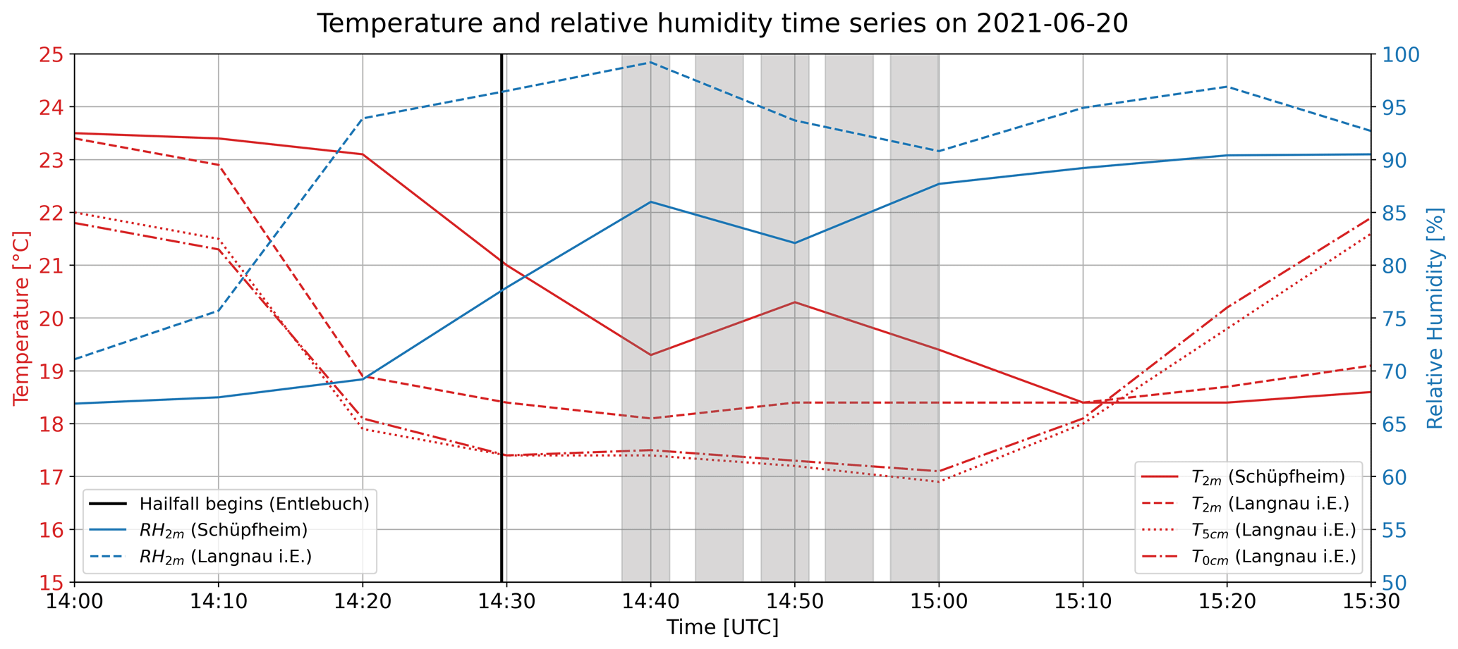
Figure 15Measurement time series of temperature (red lines) at 2 m (T2 m), 5 cm (T5 cm) and ground level (T0 cm) and relative humidity (blue lines) at 2 m (RH2 m) from the SwissMetNet (SMN) weather station in Langnau i.E. (744 ) and measurement time series of T2 m and RH2 m from the SMN weather station in Schüpfheim (744 ) on 20 June 2021 between 14:00 and 15:30 UTC. The beginning of the hail fall in Entlebuch is marked as a vertical black line, and the durations of the drone flights to capture the soccer middle circle are marked as gray-shaded bars.
In the time series plot of Fig. 15, the evolution of temperature and relative humidity for two SwissMetNet (SMN) weather stations (Schüpfheim and Langnau i.E.) is shown between 14:00 and 15:30 UTC alongside the time information about the drone flights and the beginning of hail fall at the soccer field in Entlebuch. The stations are located at a distance of 5.7 km (Schüpfheim) and 20 km (Langnau i.E.) from the soccer field. Unfortunately, no in situ measurements are available for this event. The closest precipitation measurements from an automatic rain gauge (Entlebuch station) are available at a distance of 670 m to the east. Between 14:30 and 14:40 UTC, 9.1 mm was recorded, and 0.2 mm was recorded in the subsequent 10 min. Thus, the hail on the ground was exposed to strong rain, which might have affected the melting rate. At the same time, temperatures close to the ground decreased by about 4.5 °C between 14:00 and 14:30 UTC, after the supercell passed the SMN station Langnau i.E.. The temperature drop at the soccer field is assumed to be of a similar magnitude. To better assess the melting process, future drone-based hail surveys should include a mobile weather station or some ground temperature sensors at the observation site.
Reliable ground truth data from hail observations are rare and of high value to the hail research community. This paper assesses an application of aerial drone-based photogrammetry combined with a state-of-the-art deep learning object detection model to retrieve the hail size distribution over a large area. The HSD retrieved from a large survey area allows for the capturing of a representative distribution and can thus serve as a complementary source to existing ground-based observation networks such as automatic hail sensors and crowdsourced reports.
During a period in June 2021, exceptionally strong convective storms occurred in Switzerland. On 20 June 2021 drone-based photogrammetric data of a hail event related to a right-moving supercell were collected near Entlebuch (canton of Lucerne, Switzerland). Five successive drone-based photogrammetry flights were performed above a soccer field between 14:38 and 15:00 UTC. A deep learning instance segmentation model (Mask R-CNN) under the Detectron2 framework was trained to automatically retrieve the hail size distribution.
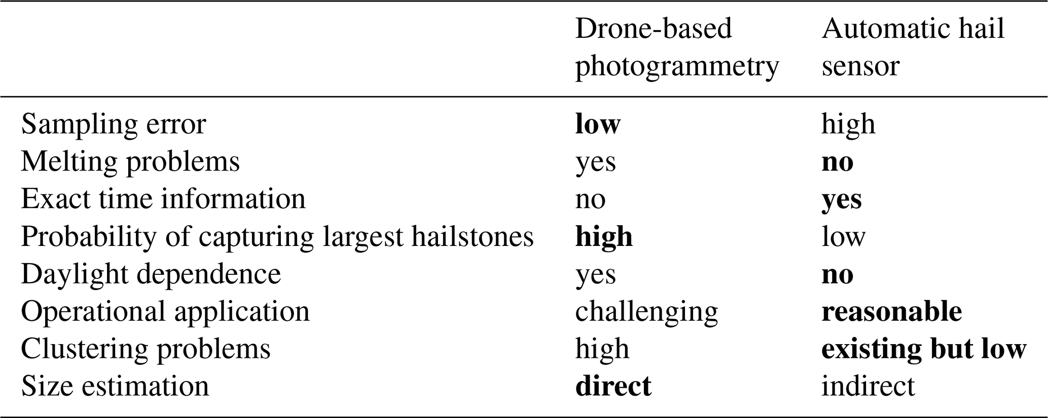
Table 4Advantages (bold) and disadvantages (normal font) of the two hail observation methods: drone-based photogrammetry and automatic hail sensor.
The key results and conclusions are listed below:
-
A robust retrieval of an HSD based on 18 207 hailstones on an area of 750.4 m2 from a single hail event with a duration of about 9.5 min is presented. The median hailstone size was 9 mm, and the majority of hailstones were rather spherical, with axis ratios greater than 0.9.
-
The largest hailstone was 39 mm and is substantially larger than estimates retrieved from nearby automatic hail sensors.
-
A combination of hail data from different sources (drone, automatic hail sensors and crowdsourced reports) used to observe hail on the ground improves the reconstruction of the complete HSD and allows for the assessment of the limitations of each method. Furthermore, such ground truth data can help to verify and further develop radar-based hail estimations.
-
The analysis of virtual hail sensors placed in the photogrammetric data highlights the challenge of observing a representative sample of the HSD using a device with an area (0.2 m2) much smaller than a typical hail swath.
-
The evolution of the HSD caused by melting could be monitored during a period of 18.65 min by analyzing data from multiple drone flights. A melting rate on the order of 0.5 mm min−1 could be estimated.
Radar-based hail algorithms estimating the size of hail, such as MESHS, need ground-based measurements for verification and potential improvements. Drone-based photogrammetry can cover areas closer to the radar spatial resolution, which makes this approach particularly valuable for the verification of radar products.
The comparison of drone-based photogrammetry with automatic hail sensors allowed for the highlighting of the advantages and limitations of both approaches in measuring hail (see Table 4 for a summary). Here, we want to highlight that the clustering problem refers to many hailstones that aggregate on the ground next to each other. This predominantly occurs during hail events with dominating small hail and intense precipitation. The resulting hail clusters pose a problem for the algorithm regarding differentiating between individual hailstones. An equivalent problem within the automatic hail sensor data is related to the dead time after each hail impact. The dead time is necessary to avoid any interference with subsequent impacts and to perform the retrieval of the data (Kopp et al., 2023). Furthermore, combining data from both approaches strongly improves the reconstruction of the complete HSD and could further extend our understanding of hailstorms.
Future drone-based photogrammetry of hail could be improved by having an artificial light source. Poor light conditions are the main challenge caused by the thunderstorm itself or if the hail occurs during twilight or at night. The light conditions determine the exposure time which limits the maximum flight velocity to keep the motion blur at the same level. A flash or an additional light source allows for increased flight velocity, and thus a larger area can be covered. In addition, the image quality can be improved by reducing the sensor gain (ISO) and the aperture size. Other ideas to test and potentially improve the techniques in the future are
-
the integration of thermal imagery to help exclude or include potential hailstones alongside the RGB image processing,
-
the usage of SfM (structure-from-motion) results and application of Mask R-CNN directly to mesh or point clouds instead to the RGB orthophotos,
-
the fine-tuning of hardware settings and flight characteristics for optimal image quality in conjunction with an acceptable motion blur.
To further assess the hail size distribution of different storms, more observational data are crucial. However, the collection of drone-based aerial photography of hail is a time-consuming and challenging task. Therefore, it could be beneficial to set up a public database of performed drone-based hail surveys to enhance collaborations between different research groups on the adaptation and testing of existing algorithms for various hail events. Moreover, with the increasing use of personal drones equipped with cameras, there could be a public community that brings the basic requirements for such observations. It might thus be useful to provide the information about how to collect adequate image data and collect such data using a crowdsourced approach similar to the existing crowdsourced reporting systems at weather services (e.g., Federal Office for Meteorology and Climatology, MeteoSwiss, or the German Weather Service, DWD). Another point to address is tests with artificial hail objects of defined size classes with different backgrounds. In this way, several setups could be trained, tested and optimized: safe drone operation in various conditions, flight missions and camera settings and precise comparison of the retrieved HSD to the known ground truth.
The data collections from the hail event on 20 June 2021 analyzed in this work are publicly available at https://doi.org/10.5281/zenodo.10609730 (Lainer, 2024).
ML performed the following roles: conceptualization, methodology, software, validation, hail annotation, formal analysis, visualization and writing the original draft. KPB performed the following roles: conceptualization, methodology, storm chasing, drone operations, review and editing. AH performed the following roles: PI hail sensors, review and editing. JK performed the following roles: automatic hail sensor data preparation, review and editing. SM performed the following roles: conceptualization, methodology, storm chasing, hail annotation, review and editing, and project administration. DW performed the following roles: conceptualization, methodology, hail annotation, review and editing. UG performed the following roles: initiation of hail research projects, acquisition of funding, procurement of equipment, review and editing.
The contact author has declared that none of the authors has any competing interests.
Publisher’s note: Copernicus Publications remains neutral with regard to jurisdictional claims made in the text, published maps, institutional affiliations, or any other geographical representation in this paper. While Copernicus Publications makes every effort to include appropriate place names, the final responsibility lies with the authors.
Hail is a severe threat to the society, and ongoing research is important to be able to establish risk mitigation measures. In this context, we thank the Swiss insurance company La Mobilière for funding the installation and operation of the automatic hail sensor network and for making the hail sensor data available for research investigations. We want to acknowledge the fruitful scientific exchange with Joshua Soderholm (Australian Bureau of Meteorology) about drone-based hail photogrammetry.
This paper was edited by Pavlos Kollias and reviewed by Andrew McMahon and three anonymous referees.
Allen, J. T., Giammanco, I. M., Kumjian, M. R., Jurgen Punge, H., Zhang, Q., Groenemeijer, P., Kunz, M., and Ortega, K.: Understanding Hail in the Earth System, Rev. Geophys., 58, e2019RG000665, https://doi.org/10.1029/2019RG000665, 2020. a
Barras, H., Hering, A., Martynov, A., Noti, P.-A., Germann, U., and Martius, O.: Experiences with > 50,000 Crowdsourced Hail Reports in Switzerland, B. Am. Meteorol. Soc., 100, 1429–1440, https://doi.org/10.1175/BAMS-D-18-0090.1, 2019. a, b
Bemis, S. P., Micklethwaite, S., Turner, D., James, M. R., Akciz, S., Thiele, S. T., and Bangash, H. A.: Ground-based and UAV-Based photogrammetry: A multi-scale, high-resolution mapping tool for structural geology and paleoseismology, J. Struct. Geol., 69, 163–178, https://doi.org/10.1016/j.jsg.2014.10.007, 2014. a
Bradski, G.: The OpenCV Library, Dr. Dobb's Journal of Software Tools, 2236121, https://www.drdobbs.com/open-source/the-opencv-library/184404319 (last access: 26 April 2024), 2000. a, b
Brook, J. P., Protat, A., Soderholm, J., Carlin, J. T., McGowan, H., and Warren, R. A.: HailTrack – Improving Radar-Based Hailfall Estimates by Modeling Hail Trajectories, J. Appl. Meteorol. Clim., 60, 237–254, https://doi.org/10.1175/JAMC-D-20-0087.1, 2021. a
Bunkers, M. J., Klimowski, B. A., Zeitler, J. W., Thompson, R. L., and Weisman, M. L.: Predicting Supercell Motion Using a New Hodograph Technique, Weather Forecast., 15, 61–79, https://doi.org/10.1175/1520-0434(2000)015<0061:PSMUAN>2.0.CO;2, 2000. a
Chronis, T., Carey, L. D., Schultz, C. J., Schultz, E. V., Calhoun, K. M., and Goodman, S. J.: Exploring Lightning Jump Characteristics, Weather Forecast., 30, 23–37, https://doi.org/10.1175/WAF-D-14-00064.1, 2015. a
Fawcett, D., Azlan, B., Hill, T. C., Kho, L. K., Bennie, J., and Anderson, K.: Unmanned aerial vehicle (UAV) derived structure-from-motion photogrammetry point clouds for oil palm (Elaeis guineensis) canopy segmentation and height estimation, Int. J. Remote Sens., 40, 7538–7560, https://doi.org/10.1080/01431161.2019.1591651, 2019. a
Feldmann, M., Hering, A., Gabella, M., and Berne, A.: Hailstorms and rainstorms versus supercells – a regional analysis of convective storm types in the Alpine region, npj Clim. Atmos. Sci., 6, 19, https://doi.org/10.1038/s41612-023-00352-z, 2023. a
Fraile, R., Castro, A., and Sánchez, J.: Analysis of hailstone size distributions from a hailpad network, Atmos. Res., 28, 311–326, https://doi.org/10.1016/0169-8095(92)90015-3, 1992. a
Fraile, R., Castro, A., López, L., Sánchez, J. L., and Palencia, C.: The influence of melting on hailstone size distribution, Atmos. Res., 67–68, 203–213, https://doi.org/10.1016/S0169-8095(03)00052-8, 2003. a
Germann, U., Boscacci, M., Clementi, L., Gabella, M., Hering, A., Sartori, M., Sideris, I. V., and Calpini, B.: Weather Radar in Complex Orography, Remote Sens., 14, 503, https://doi.org/10.3390/rs14030503, 2022. a, b
Goutte, C. and Gaussier, E.: A Probabilistic Interpretation of Precision, Recall and F-Score, with Implication for Evaluation, in: Advances in Information Retrieval, edited by: Losada, D. E. and Fernández-Luna, J. M., Springer Berlin Heidelberg, Berlin, Heidelberg, 345–359, https://doi.org/10.1007/978-3-540-31865-1_25, 2005. a
Guidi, G., Shafqat Malik, U., and Micoli, L. L.: Optimal Lateral Displacement in Automatic Close-Range Photogrammetry, Sensors, 20, 6280, https://doi.org/10.3390/s20216280, 2020. a
He, K., Zhang, X., Ren, S., and Sun, J.: Deep Residual Learning for Image Recognition, in: 2016 IEEE Conference on Computer Vision and Pattern Recognition (CVPR), Las Vegas, NV, USA, 27–30 June 2016, IEEE, 770–778, https://doi.org/10.1109/CVPR.2016.90, 2016. a
He, K., Gkioxari, G., Dollár, P., and Girshick, R.: Mask R-CNN, IEEE T. Pattern Anal., 42, 386–397, https://doi.org/10.1109/TPAMI.2018.2844175, 2020. a
Hering, A., Morel, C., Galli, G., Sénési, S., Ambrosetti, P., and Boscacci, M.: Nowcasting thunderstorms in the Alpine region using a radar based adaptive thresholding scheme, in: Proceedings of the 3rd European Conference on Radar in Meteorology and Hydrology, Visby, Island of Gotland, Sweden, 6–10 September 2004, Copernicus GmbH, ISBN 3936586292, ISBN 9783936586299, 2004. a
Houze, R. A., Schmid, W., Fovell, R. G., and Schiesser, H.-H.: Hailstorms in Switzerland: Left Movers, Right Movers, and False Hooks, Mon. Weather Rev., 121, 3345–3370, https://doi.org/10.1175/1520-0493(1993)121<3345:HISLMR>2.0.CO;2, 1993. a
Knight, N. C.: Hailstone Shape Factor and Its Relation to Radar Interpretation of Hail, J. Clim. Appl. Meteorol., 25, 1956–1958, http://www.jstor.org/stable/26183454 (last access: 12 December 2023), 1986. a, b, c, d
Kopp, J., Schröer, K., Schwierz, C., Hering, A., Germann, U., and Martius, O.: The summer 2021 Switzerland hailstorms: weather situation, major impacts and unique observational data, Weather, 78, 184–191, https://doi.org/10.1002/wea.4306, 2022. a, b
Kopp, J., Manzato, A., Hering, A., Germann, U., and Martius, O.: How observations from automatic hail sensors in Switzerland shed light on local hailfall duration and compare with hailpad measurements, Atmos. Meas. Tech., 16, 3487–3503, https://doi.org/10.5194/amt-16-3487-2023, 2023. a, b
Kumjian, M. R. and Lombardo, K.: A Hail Growth Trajectory Model for Exploring the Environmental Controls on Hail Size: Model Physics and Idealized Tests, J. Atmos. Sci., 77, 2765–2791, https://doi.org/10.1175/JAS-D-20-0016.1, 2020. a
Kumjian, M. R. and Ryzhkov, A. V.: Polarimetric Signatures in Supercell Thunderstorms, J. Appl. Meteorol. Clim., 47, 1940–1961, https://doi.org/10.1175/2007JAMC1874.1, 2008. a
Lainer, M.: Hail Event on 2021-06-20 in Entlebuch (LU), Switzerland: Drone Photogrammetry Imagery, Hail Sensor Recordings, Mask R-CNN Model and Analysis Data of Hailstones, Zenodo [data set], https://doi.org/10.5281/zenodo.10609730, 2024. a
la Mobilière: 2021 Annual Report in brief, Tech. rep., Mobilière Holding Ltd., Berne, https://report.mobiliar.ch/2021/app/uploads/2022/03/mobiliar_ar21_in-brief.pdf (last access: 26 April 2024), 2021. a
Lin, T.-Y., Maire, M., Belongie, S., Bourdev, L., Girshick, R., Hays, J., Perona, P., Ramanan, D., Zitnick, C. L., and Dollár, P.: Microsoft COCO: Common Objects in Context, arXiv [preprint], https://doi.org/10.48550/arxiv.1405.0312, 1 May 2014. a
Löffler-Mang, M., Schön, D., and Landry, M.: Characteristics of a new automatic hail recorder, Atmos. Res., 100, 439–446, https://doi.org/10.1016/j.atmosres.2010.10.026, 2011. a
mapillary: OpenSfM, GitHub [code], https://github.com/mapillary/OpenSfM (last access: 15 April 2024), 2020. a
mapillary: OpenSFM, GitHub [code], https://github.com/mapillary/OpenSfM/blob/main/README.md (last access: 15 April 2024), 2023. a
May, R. M., Arms, S. C., Marsh, P., Bruning, E., Leeman, J. R., Goebbert, K., Thielen, J. E., Bruick, Z. S., and Camron, M. D.: MetPy: A Python Package for Meteorological Data, Unidata [data set], https://doi.org/10.5065/D6WW7G29, 2023. a
Najman, L. and Schmitt, M.: Watershed of a continuous function, Signal Process., 38, 99–112, https://doi.org/10.1016/0165-1684(94)90059-0, 1994. a
Nisi, L., Martius, O., Hering, A., Kunz, M., and Germann, U.: Spatial and temporal distribution of hailstorms in the Alpine region: a long-term, high resolution, radar-based analysis, Q. J. Roy. Meteor. Soc., 142, 1590–1604, https://doi.org/10.1002/qj.2771, 2016. a
Nisi, L., Hering, A., Germann, U., and Martius, O.: A 15-year hail streak climatology for the Alpine region, Q. J. Roy. Meteor. Soc., 144, 1429–1449, https://doi.org/10.1002/qj.3286, 2018. a
Nisi, L., Hering, A., Germann, U., Schroeer, K., Barras, H., Kunz, M., and Martius, O.: Hailstorms in the Alpine region: Diurnal cycle, 4D-characteristics, and the nowcasting potential of lightning properties, Q. J. Roy. Meteor. Soc., 146, 4170–4194, https://doi.org/10.1002/qj.3897, 2020. a
OpenDroneMap: ODM – A command line toolkit to generate maps, point clouds, 3D models and DEMs from drone, balloon or kite images, GitHub [code], https://github.com/OpenDroneMap/ODM (last access: 1 April 2024), 2020. a
Powers, D. M. W.: Evaluation: from precision, recall and F-measure to ROC, informedness, markedness and correlation, CoRR, arXiv [preprint], https://doi.org/10.48550/arXiv.2010.16061, 11 October 2020. a
Rasmussen, R. and Pruppacher, H. R.: A Wind Tunnel and Theoretical Study of the Melting Behavior of Atmospheric Ice Particles. I: A Wind Tunnel Study of Frozen Drops of Radius < 500 µm, J. Atmos. Sci., 39, 152–158, https://doi.org/10.1175/1520-0469(1982)039<0152:AWTATS>2.0.CO;2, 1982. a
Rasmussen, R. M. and Heymsfield, A. J.: Melting and Shedding of Graupel and Hail. Part I: Model Physics, J. Atmos. Sci., 44, 2754–2763, https://doi.org/10.1175/1520-0469(1987)044<2754:MASOGA>2.0.CO;2, 1987. a
Romppainen-Martius, O.: The Swiss Hail Network, Mobiliar Lab for Natural Risks, University of Bern, https://www.mobiliarlab.unibe.ch/research/applied_research_on_hail_and_wind_gusts/the_swiss_hail_network/index_eng.html (last access: 26 February 2024), 2022. a
Schmidhuber, J.: Deep learning in neural networks: An overview, Neural Networks, 61, 85–117, https://doi.org/10.1016/j.neunet.2014.09.003, 2015. a
Schultz, C. J., Petersen, W. A., and Carey, L. D.: Preliminary Development and Evaluation of Lightning Jump Algorithms for the Real-Time Detection of Severe Weather, J. Appl. Meteorol. Clim., 48, 2543–2563, https://doi.org/10.1175/2009JAMC2237.1, 2009. a
Sekachev, B., Manovich, N., Zhiltsov, M., Zhavoronkov, A., Kalinin, D., Hoff, B., TOsmanov, Kruchinin, D., Zankevich, A., DmitriySidnev, Markelov, M., Johannes222, Chenuet, M., a andre, telenachos, Melnikov, A., Kim, J., Ilouz, L., Glazov, N., Priya4607, Tehrani, R., Jeong, S., Skubriev, V., Yonekura, S., vugia truong, zliang7, lizhming, and Truong, T.: opencv/cvat: v1.1.0, Zenodo [code], https://doi.org/10.5281/zenodo.4009388, 2020. a
Shedd, L., Kumjian, M. R., Giammanco, I., Brown-Giammanco, T., and Maiden, B. R.: Hailstone Shapes, J. Atmos. Sci., 78, 639–652, https://doi.org/10.1175/JAS-D-20-0250.1, 2021. a, b, c, d, e
Soderholm, J. S., Kumjian, M. R., McCarthy, N., Maldonado, P., and Wang, M.: Quantifying hail size distributions from the sky – application of drone aerial photogrammetry, Atmos. Meas. Tech., 13, 747–754, https://doi.org/10.5194/amt-13-747-2020, 2020. a, b, c, d, e, f, g, h, i
SwissGeoportal: https://map.geo.admin.ch/ (last access: 15 April 2024), 2023. a
Treloar, A.: Vertically integrated radar reflectivity as an indicator of hail size in the greater Sydney region of Australia, in: Preprints, 19th Conf. on Severe Local Storms, Minneapolis, MN, USA, 14–18 September 1998, Amer. Meteor. Soc, 48–51, 1998. a
Van Rijsbergen, C. J.: Information retrieval, 2nd edn., Butterworths, Newton, Ma, ISBN 9780408709293, 1979. a
Waldvogel, A., Federer, B., and Grimm, P.: Criteria for the Detection of Hail Cells, J. Appl. Meteorol. Clim., 18, 1521–1525, https://doi.org/10.1175/1520-0450(1979)018<1521:CFTDOH>2.0.CO;2, 1979. a
Wilks, D. S.: Statistical methods in the atmospheric sciences, vol. 100, Academic press, ISBN 9780123850225, 2011. a
Wu, Y., Kirillov, A., Massa, F., Lo, W.-Y., and Girshick, R.: Detectron2, GitHub [code], https://github.com/facebookresearch/detectron2 (last access: 20 March 2024), 2019. a
Wu, Y., Kirillov, A., Massa, F., Lo, W.-Y., and Girshick, R.: Detectron2, GitHub [code], https://github.com/facebookresearch/detectron2/blob/main/detectron2/config/defaults.py (last access: 20 March 2024), 2023. a
Ziegler, C. L., Ray, P. S., and Knight, N. C.: Hail Growth in an Oklahoma Multicell Storm, J. Atmos. Sci., 40, 1768–1791, https://doi.org/10.1175/1520-0469(1983)040<1768:HGIAOM>2.0.CO;2, 1983. a
Zou, Z., Shi, Z., Guo, Y., and Ye, J.: Object Detection in 20 Years: A Survey, arXiv [preprint], https://doi.org/10.48550/arxiv.1905.05055, 13 May 2019. a