Intercomparison of eddy-covariance software for urban tall-tower sites

Long-term tall-tower eddy-covariance (EC) measurements have been recently established in three European pilot cities as part of the ICOS-Cities project. We conducted a comparison of EC software to ensure a reliable generation of interoperable flux estimates, which is the prerequisite for avoiding methodological biases and improving the comparability of the results. We analyzed datasets covering 5 months collected from EC tall-tower installations located in urbanized areas of Munich, Zurich, and Paris. Fluxes of sensible heat, latent heat, and CO₂ were calculated using three software packages (i.e., TK3, EddyPro, and eddy4R) to assess the uncertainty of flux estimations attributed to differences in implemented postprocessing schemes. A very good agreement on the mean values and standard deviations was found across all three sites, which can probably be attributed to a uniform instrumentation, data acquisition, and preprocessing. The overall comparison of final flux time series products showed a good but not yet perfect agreement among the three software packages. TK3 and EddyPro both calculated fluxes with low-frequency spectral correction, resulting in better agreement than between TK3 and the eddy4R workflow with disabled low-frequency spectral treatment. These observed flux discrepancies indicate the crucial role of treating low-frequency spectral loss in flux estimation for tall-tower EC systems.

1 Introduction

While urban areas cover only a minuscule fraction of the Earth's terrestrial area, approximately 3 % as reported by Liu et al. (2014), they are home to more than 55 % of the global population, thereby exerting a substantial influence on global greenhouse gas (GHG) emissions (IPCC, 2022). The continued expansion of urban areas is projected to accommodate an estimated 68 % (approximately 6.7 billion people) of the world's population by 2050, driven by the ongoing trend of urbanization (UN, 2019). Hence, the pivotal role of urban areas in contributing to global CO₂ emissions is widely acknowledged. This recognition has not only accelerated the development of climate action plans (e.g., Liu et al., 2022; C-40, 2022; European Commission, 2022; Jenkins et al., 2021) but also raised growing interest in existing observation techniques to verify, monitor, and improve estimates of urban CO₂ emissions. In addition to satellite observation approaches and modeling frameworks, urban eddy-covariance (EC) towers have emerged as a valuable tool for directly monitoring the exchange of CO₂ between the land surface and atmosphere with high spatial-temporal resolution (e.g., Vogt et al., 2006; Christen et al., 2011; Järvi et al., 2012; Menzer and McFadden, 2017; Lin et al., 2018; Stagakis et al., 2019). Complementing the ecosystem-focused component of the ICOS network (https://www.icos-cp.eu/observations/ecosystem, last access: 2 May 2024) in Europe, more than 15 sites (Table 1), primarily newly established, have been deployed in urban areas (Biraud and Chen, 2021; Nicolini et al., 2022). Synergies with urban networks, including the US DOE Urban Integrated Field Laboratories (https://ess.science.energy.gov/urban-ifls/, last access: 2 May 2024) and the Urban Flux Network, are established and aim to measure urban emissions and investigate the underlying processes contributing to the diurnal and seasonal patterns of the overall CO₂ balance. Within the ICOS-Cities project (https://www.icos-cp.eu/projects/icos-cities, last access: 2 May 2024), three additional cities, Munich, Zurich, and Paris, have been equipped with state-of-art EC measurement instruments.

Table 1 List of the urban EC towers within the ICOS network (http://www.europe-fluxdata.eu, last access: 2 May 2024). Tall EC towers established for the ICOS-Cities project are specified. The normalized measurement height (with urban canopy height, h_c) for the tower EC systems in the ICOS-Cities project is provided.

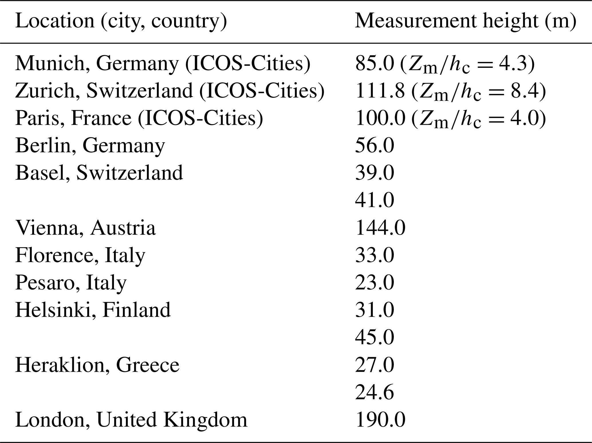
Compared to the mature ecosystem EC networks, the capacity of tall-tower EC to provide reliable estimates of urban CO₂ fluxes remains uncertain due to the paucity of pertinent observations. At the present, there are only a few published examples of tall-tower (e.g., with height reaching the inertial sublayer) urban EC measurements, including London, UK (Helfter et al., 2016); Saika, Japan (Ueyama and Ando, 2016); Beijing, China (Cheng et al., 2018); and Vienna, Austria (Matthews and Schume, 2022). Furthermore, the final flux results presented in these studies were derived via either freely distributed software, such as TK3 and EddyPro, as employed in Cheng et al. (2018) and Matthews and Schume (2022), respectively, or self-developed processing packages, as in the case of Ueyama and Ando (2016). Although the fundamental principles and assumptions underpinning the EC technique dictate that the data processing framework (de-spiking, calculation, correction, and data quality control) should not differ across software packages, variations may arise due to the inclusion of distinct methods, as extensively discussed in the literature (Mauder et al., 2007). It is noteworthy that even when following identical processing schemes, different packages might implement them in differing sequences and iterations (Aubinet et al., 2012; Mauder and Foken, 2006). Consequently, joint efforts have been made to quantify the uncertainties stemming from various data processing methods and standardize the processing methodology (Aubinet et al., 2012; Lee et al., 2004; Mauder et al., 2007, 2008, 2013; Fratini and Mauder, 2014; Mammarella et al., 2016; Sabbatini et al., 2018). It has been reported that the potential for deviations in coordinate rotation and detrending methods may account for discrepancies of up to 15 % in sensible and latent heat fluxes, while different high-frequency spectral correction schemes resulted in a 10 % discrepancy in CO₂ fluxes (Rannik and Vesala, 1999; Moncrieff et al., 2004; Mauder et al., 2007, 2008). A comprehensive intercomparison between TK3 and EddyPro, conducted by developers with in-depth knowledge of the EC method and access to the source code, revealed that disparities in final fluxes could be minimized through consistent configuration of processing steps and correction schemes (Fratini and Mauder, 2014). This investigation illuminates that differences in spectral correction schemes were the primary culprit behind the most significant discrepancies in flux results which proved challenging to eliminate. This software intercomparison study highlights the importance of achieving consensus in EC postprocessing protocols to ensure robust comparability across flux measurements.

The culmination of extensive EC software intercomparison studies has significantly contributed to the establishment of a robust data processing framework for EC data derived from ICOS ecosystem stations (Sabbatini et al., 2018). However, the persistence of uncertainties in flux estimations due to differences in postprocessing methodologies remains a pivotal inquiry, particularly in the context of tall-tower EC measurements in urban areas, which is the main compass of current work. In this study, we conducted an intercomparison of friction velocity, sensible heat, latent heat, and CO₂ fluxes calculated by three software packages (i.e., TK3, EddyPro, and eddy4R) at three urban tall-tower EC sites. The primary objective was to evaluate the influence of different postprocessing schemes on the uncertainty of flux estimations. In contrast to TK3 and EddyPro, which are pre-compiled software providing ease of use through a graphical user interface with a range of pre-configured selections, eddy4R is a community-extensible family of R packages for tower, airborne, and shipborne EC data processing on the command line, with advanced features like flux mapping workflows (Metzger et al., 2017). For applications other than urban tall towers, eddy4R has previously been compared to TK3 (Metzger et al., 2012) and EddyPro (Metzger et al., 2017), with excellent agreement in both cases. Notably, eddy4R is used to harmonize data processing across 47 ecosystem EC stations operated by the National Ecological Observatory Network (NEON). For the following intercomparison, eddy4R is configured based on the NEON workflow in version 1.3.1 (referred to as eddy4R NW hereafter) with some deviations to facilitate identical data processing for this intercomparison. A range of other workflows and methods are available, including wavelet-based low-frequency flux inclusion, storage flux, and vertical flux divergence. While such configurations were deemed outside the scope of the current study, they have been used extensively in prior tall-tower and urban research (e.g., Drysdale et al., 2022; Vaughan et al., 2021; Xu et al., 2017, 2018). Here, we focus on a baseline intercomparison of widely accepted turbulence processing schemes as a foundation for future work on low-frequency flux inclusion versus low-frequency flux correction, storage flux, and vertical flux divergence.

2 Datasets, software, and methodology

As an integral facet of the ICOS-Cities project, new tall-tower EC systems have been established in urbanized areas in three European cities: Zurich, Munich, and Paris (Fig. 1). These systems, featuring uniform instrumentation and employing standardized data acquisition methodologies, are installed on either a telecommunication tower or a meteorological tower situated on the roof of a high-rise building (Fig. 2). Specifically, three-dimensional wind velocities, sonic temperature, water vapor, and CO₂ concentrations are measured by an IRGASON (Campbell Scientific Inc.), a collocated ultrasonic anemometer, and an open-path infrared gas analyzer with a 20 Hz sampling frequency. The raw time series is collected by a CR6 datalogger (Campbell Scientific Inc.) and is subsequently streamed to our data server on an hourly basis. This exceptional level of consistency in both instrumentation and data acquisition, a rarity in many other measurement campaigns, allows us to conduct a rigorous investigation for the purpose of conducting the software intercomparison. It is expected that the outcomes of this study will primarily elucidate differences in methods adopted by different software packages or differences in the implementation of certain methods, emphasizing the importance of this comparative analysis.

Figure 1 Land cover map for the three pilot cities. The land cover map was rendered using the WorldCover product with 10 m resolution provided by European Space Agency (https://esa-worldcover.org, last access: 2 May 2024). The borders of cities and districts are denoted by thick black lines, while the location of the tall EC tower is illustrated by the white cross.

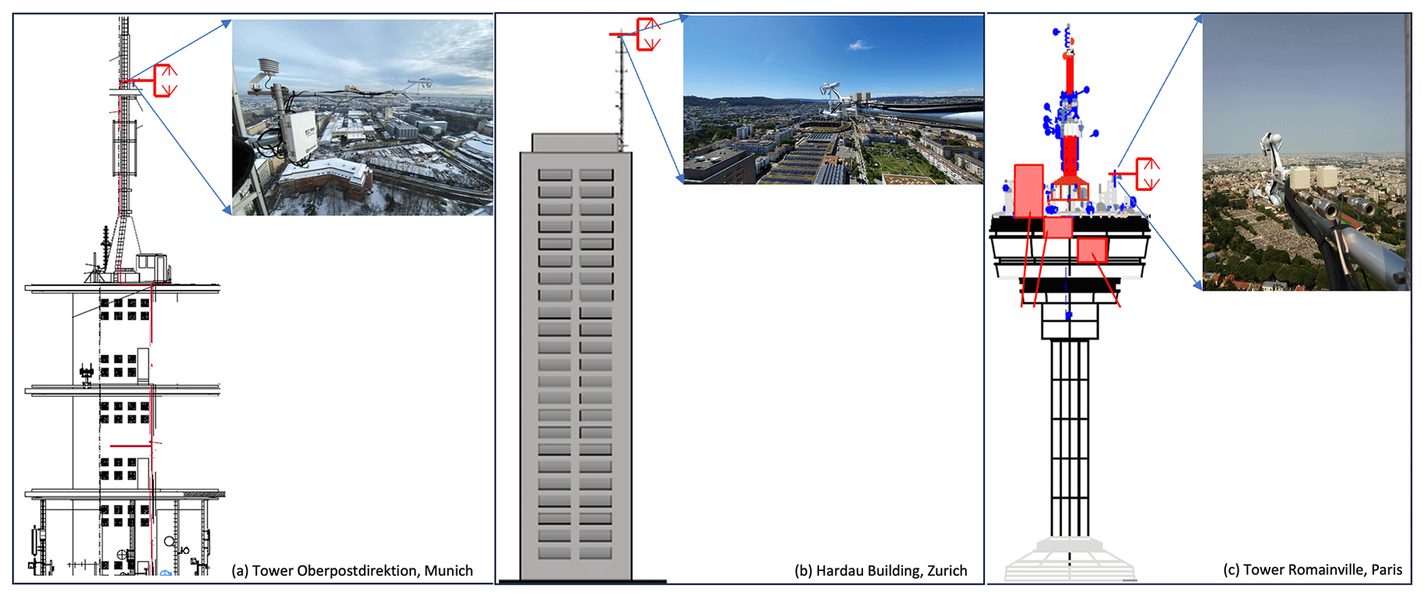
Figure 2 The schematic of the tower structure and the location of the EC system. The subpanels on the top-right are the pictures of the instrumentation taken from the tower.

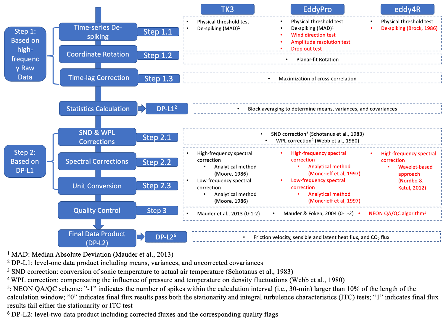
Figure 3 Processing steps of the EC software packages intercompared in this work. The overall processing chain aligns with the established protocol for CO₂ and energy flux calculations at ICOS ecosystem stations. Distinctions in configurations between EddyPro and eddy4R NEON workflow, as compared to TK3, are highlighted in red.

Before initiating the computation of fluxes using the three software packages, we subjected the initially measured raw time series to a time continuity check, which filled missing data points with “NaN” (not a number) values. This data preparation ensured that each software package processed complete daily records, thereby guaranteeing that the computed fluxes shared identical timestamps. Given that the three software packages adhered to the same combination of processing steps (Lee et al., 2004), one might anticipate that the final flux outputs would be quite similar. However, distinctions surfaced among the three software packages, not only in terms of the algorithms employed for the de-spiking process but also in their respective flux correction schemes (Fig. 3). For instance, the eddy4R NW employs the de-spiking algorithm proposed by Brock (1986) along with an additional threshold recommended by Starkenburg et al. (2016). In contrast, both TK3 and EddyPro adopt median absolute deviation (MAD) for de-spiking (Metzger et al., 2012; Mauder et al., 2013), which is also an option in eddy4R but not selected in adherence to the NEON workflow. While the Webb, Penman, and Leuning correction, called WPL (Webb et al., 1980) is used in some eddy4R studies (e.g., Wiesner et al., 2022), it is not incorporated in eddy4R NW because closed-path infrared gas analyzers (e.g., LI-7200, LI-COR Biosciences Inc.) are used at NEON ecosystem stations to measure the dry mole fraction of water vapor and CO₂. Indeed, this correction is needed for open-path infrared gas analyzers such as the IRGASON to account for the influence of pressure, temperature, and humidity on density fluctuations but accounted for in closed-path analyzers through explicit high-frequency ideal gas law conversions. Therefore, to calculate scalar fluxes from the mass density of water vapor and CO₂ measured by the IRGASON, we performed a unit conversion from mass density to dry mole fraction on the raw time series before initiating the computation (Hartmann et al., 2018). With the advantage of the collocation of the sonic anemometer and the open-path infrared gas analyzer in the IRGASON, this approach is more straightforward and has fewer artifacts compared to performing unit conversion on final fluxes. Significant distinctions also emerge in the spectral loss correction methods implemented by these three software packages. In TK3, the Moore correction is applied for spectral loss correction in both high-frequency and low-frequency ranges (Moore, 1986), while the eddy4R NW corrects only high-frequency spectral loss using a wavelet-based approach, which directly performs correction on the high-frequency time series rather than on covariances (Nordbo and Katul, 2013). A range of other high-frequency and low-frequency spectral loss treatments are available in eddy4R, such as explicit Wavelet inclusion of low-frequency fluxes (e.g., Metzger et al., 2013; Serafimovich et al., 2018; Xu et al., 2018), but were not selected for this intercomparison in adherence to eddy4R NW. As for EddyPro, it offers multiple spectral loss correction schemes, but for this study, we adopted the analytical method for both high-frequency (Moncrieff et al., 1997) and low-frequency spectral corrections (Moncrieff et al., 2004), aligning with the processing chain used for EC data measured at ICOS ecosystem sites (Sabbatini et al., 2018).

Table 2 The number of 30 min data segments assigned with different overall quality flags based on the combined results from the stationarity test and well-developed turbulence test calculated by the three software packages.

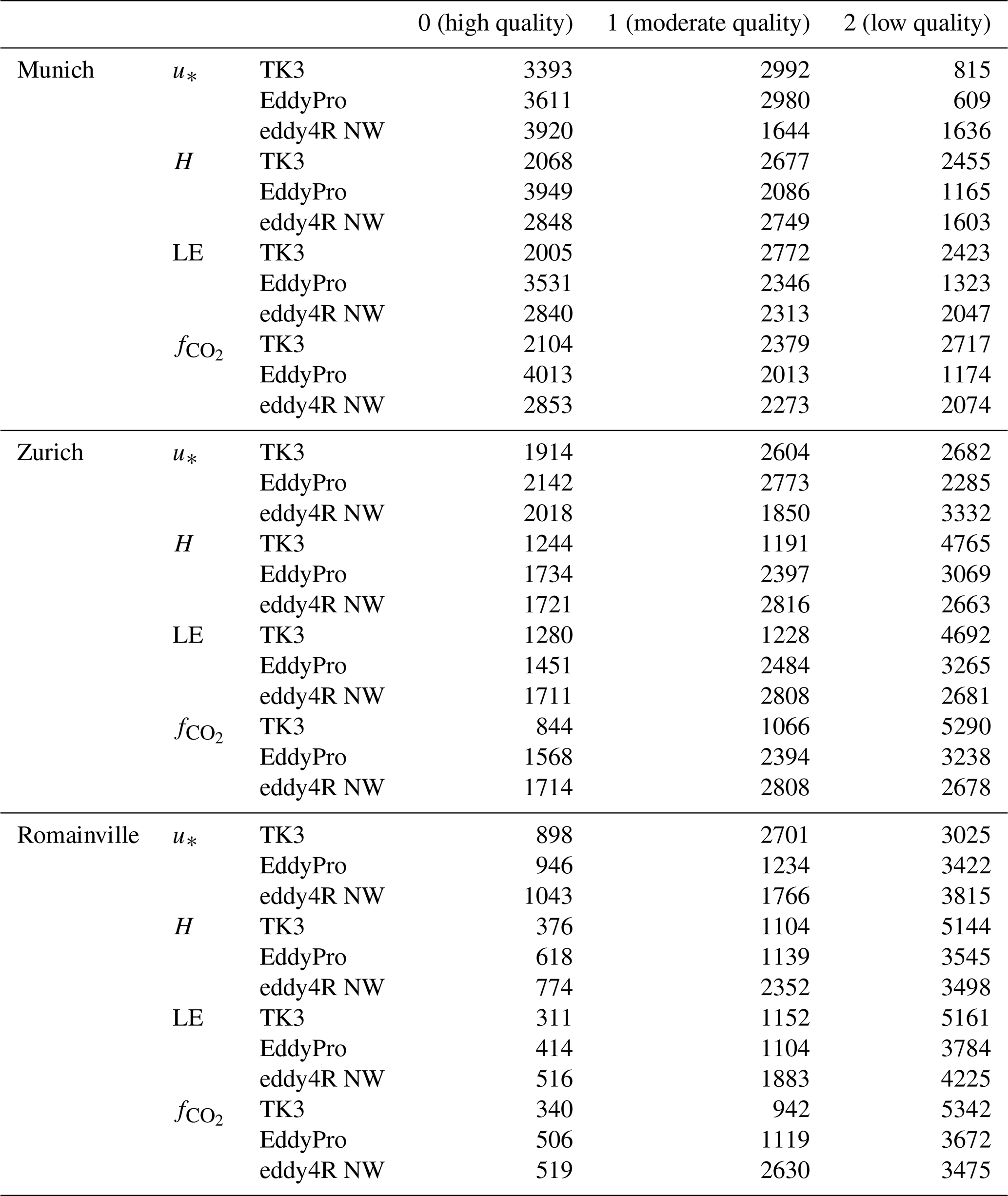
Our primary focus revolved around the intercomparison of friction velocity, sensible and latent heat fluxes, and CO₂ flux, while statistical values (i.e., mean, standard deviation, and covariance) were also considered to explain the observed discrepancies. Prior to initiating the intercomparison analysis, the fluxes were subjected to quality screening based on the “0–1–2” quality flag scheme (Mauder et al., 2013). Although the eddy4R NW applies a modular flagging scheme for cross-discipline integration in place of a traditional rank-based approach (Fig. 3), it reports the quantitative results for both the stationarity and integral turbulence characteristic tests. Hence, we utilized the quantitative test results to reassign 0–1–2 data quality flags for fluxes computed by the eddy4R NW, adhering to the methodology outlined by Mauder et al. (2013). Table 2 provides the distribution of final flux results, assigned by the overall quality flags determined through the amalgamated outcomes of the stationarity test and the well-established turbulence test for all three software packages. In addition, TK3 also applies a test for the mean w-offset after planar-fit and interdependency of flags due to corrections or conversions (Mauder et al., 2013). As revealed by prior studies, the residual differences in quality flags were mostly due to different algorithms used for the well-developed turbulence test (Foken et al., 2004; Fratini and Mauder, 2014). However, TK3 tends to classify less data as high quality (i.e., class 0), which can probably be explained by the additional tests described above. It is also interesting to note that data from the Munich site show the largest proportion of high-quality data, followed by Zurich and Paris. These differences can be interpreted as a measure for the suitability of a tower for eddy-covariance measurements. The relatively slim tower structure in the upper 40 m of the Munich tower probably generates less flow distortion than the more bulky constructions of the towers in Zurich and especially in Paris.

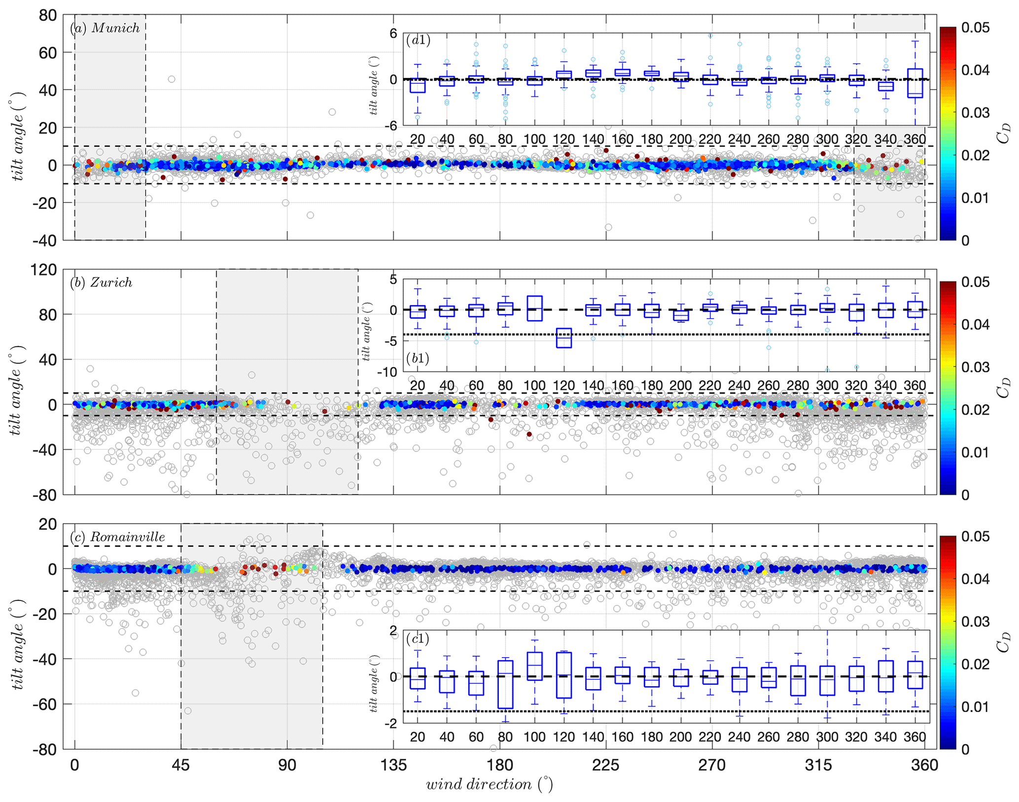
Figure 4 The distribution of tilt angle $\left(\frac{\stackrel{\mathrm{‾}}{w}}{\stackrel{\mathrm{‾}}{u}}\right)$ with respect to wind direction. The gray circles represent all data points before quality flag screening. The solid markers indicate data points assigned a “0” quality flag, with color-coding corresponding to the drag coefficient $\left(C_{\mathrm{D}}={\left(\frac{\stackrel{\mathrm{‾}}{u}}{u_{\ast }}\right)}^{\mathrm{2}}\right)$. The shaded areas denote the wind sectors ruled out due to masking effect. The boxplots (a1)–(c1) indicate the median and interquartile of tilt angle as a function of wind sectors only using data points assigned a “0” quality flag. The dotted black line indicates the mean value of all data points.

The distribution of tilt angles with respect to wind direction was also examined, with the aim of excluding data segments potentially influenced by the building wake or masking effects (Fig. 4). Notably, in contrast to the Munich site, large tilt angles were observed at the Zurich and Paris (i.e., Romainville tower) sites, implying a discernible impact of the surrounding architecture and the tower structure on the wind flow. This is likely attributed to the location of the IRGASON. Unlike the EC system in Munich, which is mounted on the needle-like structure of a telecommunication tower, the systems at the Zurich and Romainville tower sites are situated either on the rooftop of a building or on the platform of a telecom tower, which features a massive antenna on its southeastern side (Fig. 2). To minimize the masking effect and flow distortion caused by buildings, data segments with wind direction falling within ± 30° of the sonic orientation or tilt angle larger than 10° were excluded from the analysis (Ward et al., 2022; Mammarella et al., 2016). Furthermore, it was also observed that a substantial portion of fluxes corresponding to large tilt angles were marked with “1” or “2” quality levels (Fig. 4), emphasizing the importance of the turbulent stationarity test in flux quality assessment for urban EC towers. To evaluate the agreement between the fluxes computed by two different software packages, we employed the symmetric reduced major axis (RMA) linear regression. Despite TK3 not being able to generate an absolute standard of fluxes, it was designated as the reference considering its extensive validation across multiple studies using diverse datasets (Mauder et al., 2007, 2008; Fratini and Mauder, 2014).

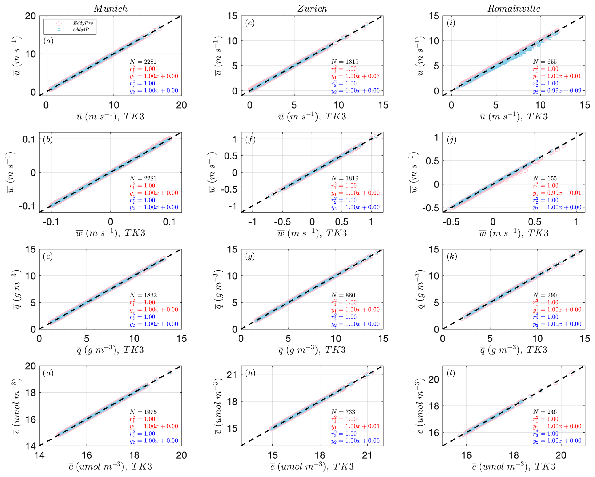
Figure 5 Comparisons of mean values estimated by the three software packages. The top-to-bottom panels represent the comparison of horizontal velocity aligned to the streamline (a, e, and i), vertical velocity (b, f, and j), mass density of water vapor (c, g, and k), and CO₂ (d, h, and l). Pink and blue markers denote the comparison between EddyPro and TK3 and between eddy4R NW and TK3, respectively. The dashed black line represents the ideal one-to-one line. The results of the regression analyses calculated by the different software packages and the corresponding number of data points are provided in the bottom-right corner of each subpanel.

Figure 6 Comparisons of the standard deviations estimated by the three software packages. The top-to-bottom panels represent the comparison of horizontal velocity aligned to the streamline (a, e, and i), vertical velocity (b, f, and j), mass density of water vapor (c, g, and k), and CO₂ (d, h, and l). Pink and blue markers denote the comparison between EddyPro and TK3 and between eddy4R NW and TK3, respectively. The dashed black line represents the ideal one-to-one line. The results of the regression analyses calculated by the different software packages and the corresponding number of data points are provided in the bottom-right corner of each subpanel.

3 Results and discussion

3.1 Comparison of mean values, standard deviation, and fluxes

We initiated the analysis by comparing mean values and standard deviations (Figs. 5 and 6; refer to Figs. B1 and B2 for the distribution of the relative difference). The regression statistics revealed a very good agreement across all three sites, which can probably be attributed to the uniformity of instrumentation, data acquisition, and preprocessing (i.e., step 1 in Fig. 3) procedures. This finding suggests that differences in de-spiking methods had minimal influence on the derived fluctuation time series, which were subsequently used to determine covariances. While no systematic differences emerged among the software packages concerning mean values and standard deviations, some data points related to vertical velocity slightly deviated from the one-to-one line. These observed deviations may be attributed to disparities in the configurations employed to derive planar-fit coefficients in TK3 and EddyPro. In TK3, data points with horizontal wind speed exceeding 5 m s⁻¹ were excluded during multiple linear regression, whereas in EddyPro, outliers were ruled out based on a user-defined threshold for maximum vertical velocity. As evidenced in Fig. 7, the 5 m s⁻¹ threshold for horizontal wind speed might not be suitable for tall-tower EC systems, as it resulted in the exclusion of nearly half of the data points when conducting multiple linear regression for determining the planar-fit coefficients. In the subsequent analysis, therefore, we conducted coordinate rotation in TK3 and eddy4R NW using the planar-fit coefficients determined by EddyPro to minimize such an influence on flux calculations.

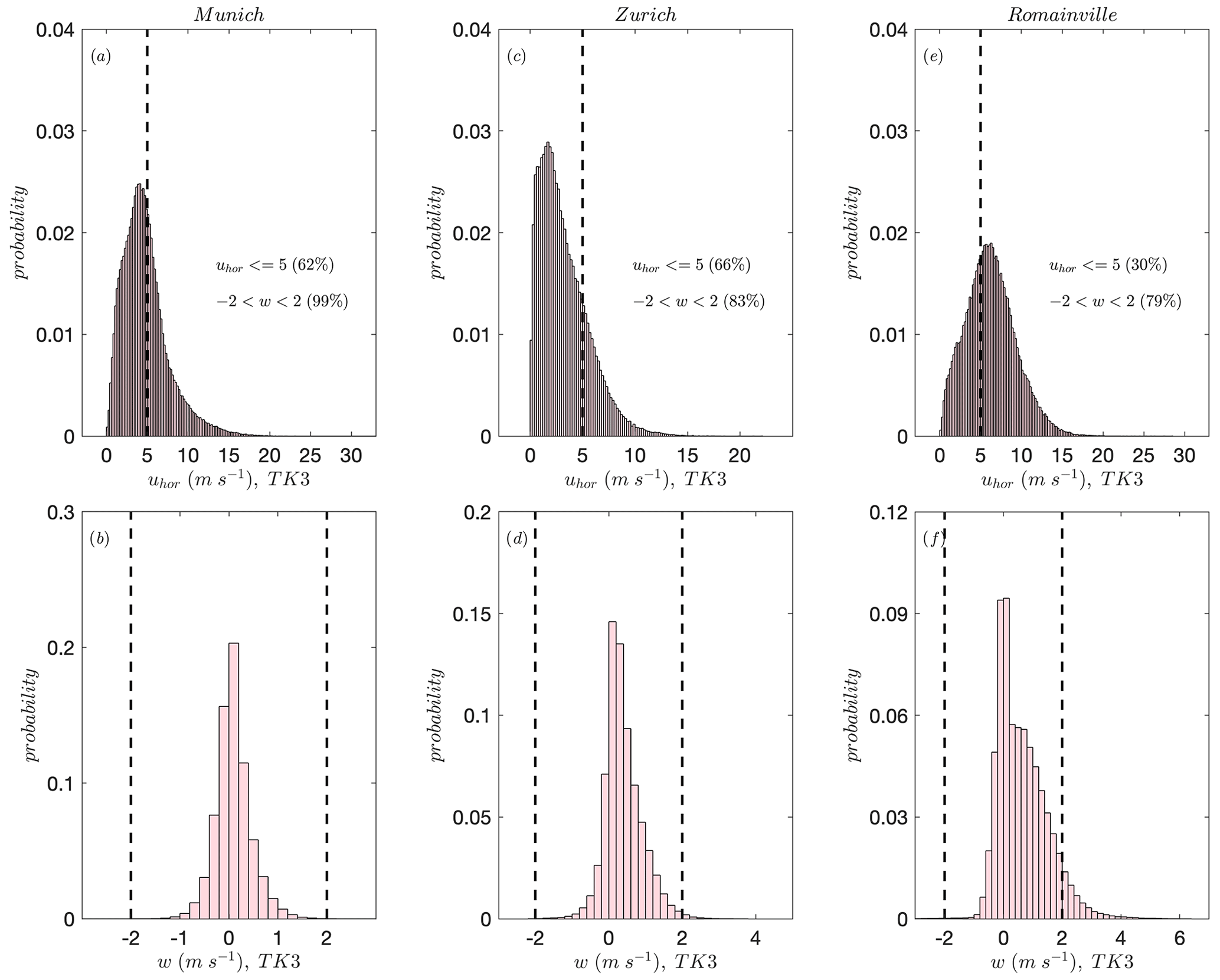
Figure 7 Histogram of probability density function for originally measured horizontal wind speed (a, c, and e) and vertical velocity (b, d, and f). In the top panels (a, c, and e), the vertical dashed line represents the threshold of horizontal wind speed configured in TK3, while in the bottom panels (b, d, and f), the vertical dashed lines represent the custom-defined range of vertical velocity in EddyPro.

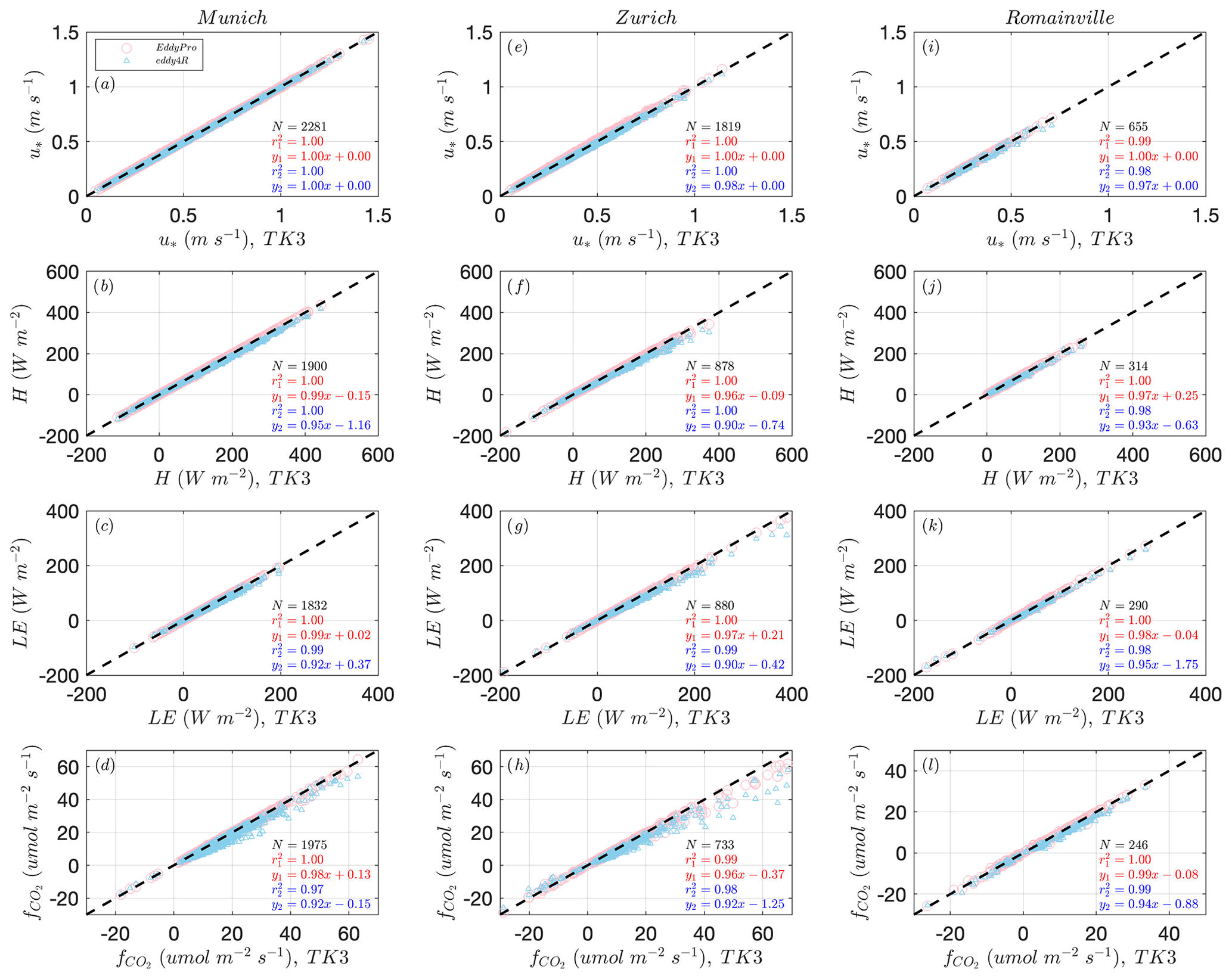
Figure 8 Comparisons of the final fluxes estimated by the three software packages. The top-to-bottom panels represent the comparison of friction velocity (a, e, and i), sensible heat flux (b, f, and j), latent heat flux (c, g, and k), and CO₂ flux (d, h, and l). Pink and blue markers denote the comparison between EddyPro and TK3 and between eddy4R NW and TK3, respectively. The dashed black line represents the ideal one-to-one line. The results of the regression analyses calculated by the different software packages and the corresponding number of data points are provided in the bottom-right corner of each subpanel.

Table 3 Summary of the root mean square error and median bias of flux results between two software packages. Note that fluxes computed by TK3 were selected as references.

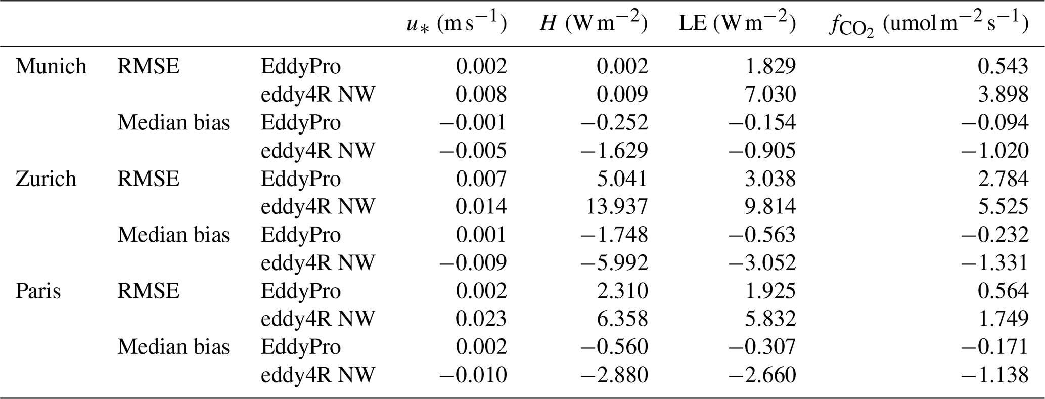
We proceeded to calculate and compare friction velocity (u_∗; Figs. 8 and B3a, e, and i), sensible heat (H; Figs. 8 and B3b, f, and j), latent heat (LE; Figs. 8 and B3c, g, and k), and CO₂ fluxes ($f_{{\mathrm{CO}}_{\mathrm{2}}}$; Figs. 8 and B3d, h, and l) at each site using the three software packages and the postprocessing configurations detailed in Fig. 3. Using the identical planar-fit coefficients, the comparison of u_∗ showed a high degree of concordance, as supported by the R² values that were near unity. However, a close agreement accompanied by systematic differences in the comparisons of energy and CO₂ fluxes was observed. Among these variables, $f_{{\mathrm{CO}}_{\mathrm{2}}}$ showed the most substantial relative bias, consistent with the findings of the prior software intercomparison study by Fratini and Mauder (2014). Additionally, both the root mean square error (RMSE) and relative bias indicated that fluxes estimated by TK3 and EddyPro were in relatively better agreement than those between TK3 and the eddy4R NW (Table 3). These findings were as expected due to the identical configurations in TK3 and EddyPro, with the exception of the spectral loss correction schemes.

3.2 Influence of spectral loss correction on fluxes

Considering that the postprocessing (i.e., de-spiking, coordinate rotation, and time-lag correction) done on the raw time series had limited impact on the uncorrected covariances, it was reasonable to expect a consistent trend in flux increments compared to the uncorrected covariance (i.e., Fig. 3, covariance in level 1 data product) if the three software packages employed an identical spectral loss correction method. However, as depicted in Fig. 9, there was a considerable variation in the relative differences between final flux results and uncorrected covariance across the three software packages. This finding confirms that the primary source of the systematic discrepancies observed in flux results (Fig. 8) can be attributed to the different spectral loss correction methods implemented in the three software packages. It is worth noting that the high-frequency spectral correction method employed by the eddy4R NW generally yielded larger correction values (order of 1 %) compared to EddyPro (order of 0.1 %). A possible advantage of the eddy4R NW wavelet-based spectral correction method, especially in non-ideal conditions, is that it is not contingent on either a theoretical cospectrum or the cospectral similarity (Nordbo and Katul, 2013). Another salient feature observed in Fig. 9 was the significant increase over the uncorrected covariances due to the low-frequency spectral loss correction, indicative of substantial flux contributed by large-scale motions detected by the tall-tower EC systems. Consequently, in contrast to short-tower EC systems, low-frequency spectral loss correction assumes a more crucial role in correcting fluxes measured by tall-tower EC systems (order of 10 %). Hence, the implementation of similar high- and low-frequency spectral loss correction schemes can explain the relatively small differences in fluxes estimated by TK3 and EddyPro. On the other hand, the disabled low-frequency spectral treatment in the eddy4R NW can explain the systematic differences in fluxes compared to TK3.

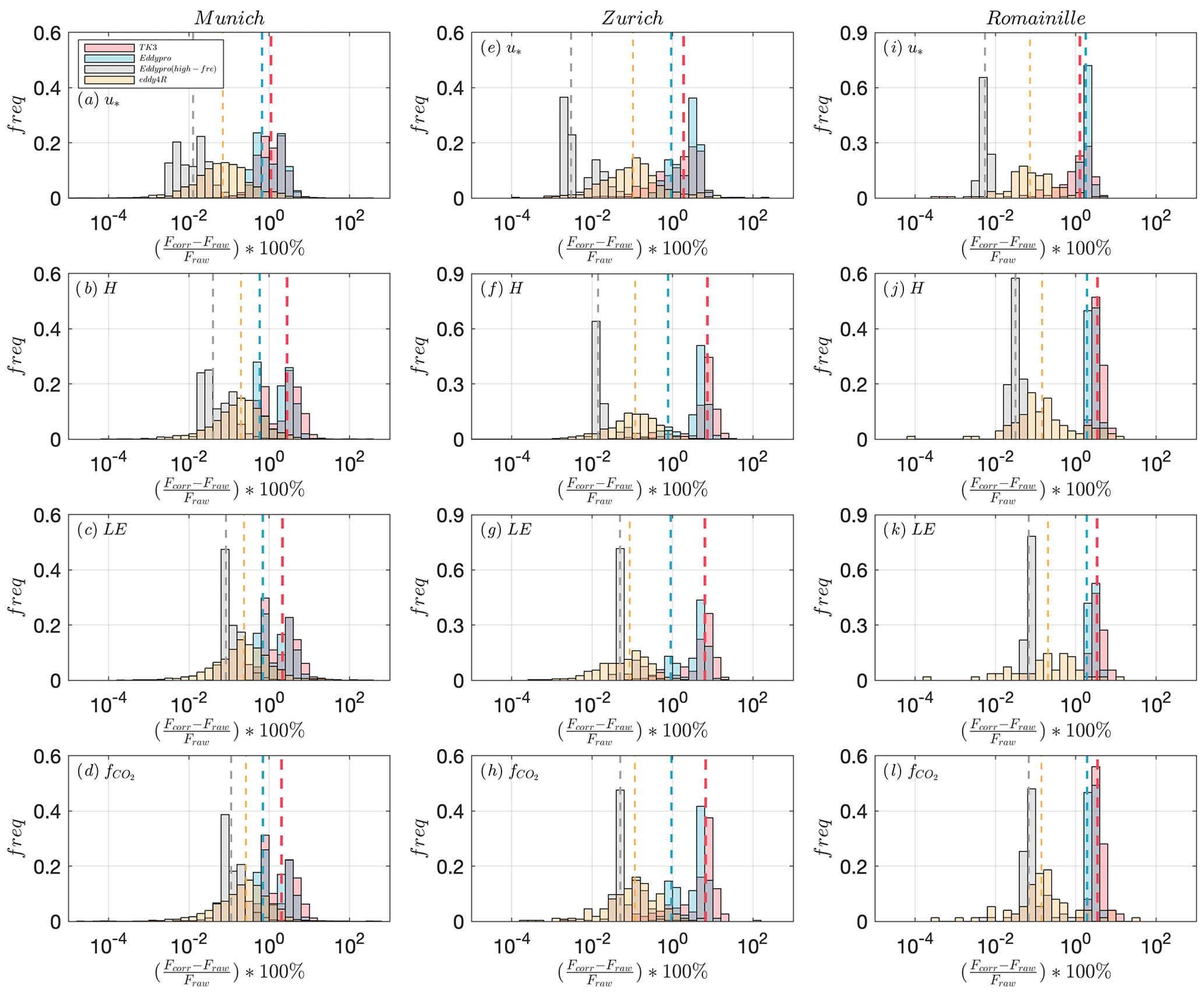
Figure 9 The frequency distribution of the relative difference between corrected flux and raw covariance. The top-to-bottom panels represent the result of friction velocity (a, e, and i), sensible heat flux (b, f, and j), latent heat flux (c, g, and k), and CO₂ flux (d, h, and l). The vertical dashed lines in red, blue, gray, and yellow represent the median values of relative differences corresponding to the results of TK3, EddyPro, EddyPro with only high-frequency spectral loss correction, and eddy4R NW, respectively.

Figure 10 Median diurnal variation in the relative bias in fluxes. The top-to-bottom panels represent the result of friction velocity (a, e, and i), sensible heat flux (b, f, and j), latent heat flux (c, g, and k), and CO₂ flux (d, h, and l). Pink and blue lines denote the relative bias in fluxes between EddyPro and TK3 and between eddy4R and TK3, respectively. The horizontal dashed line represents the zero line, indicating the estimated fluxes by two software packages are identical.

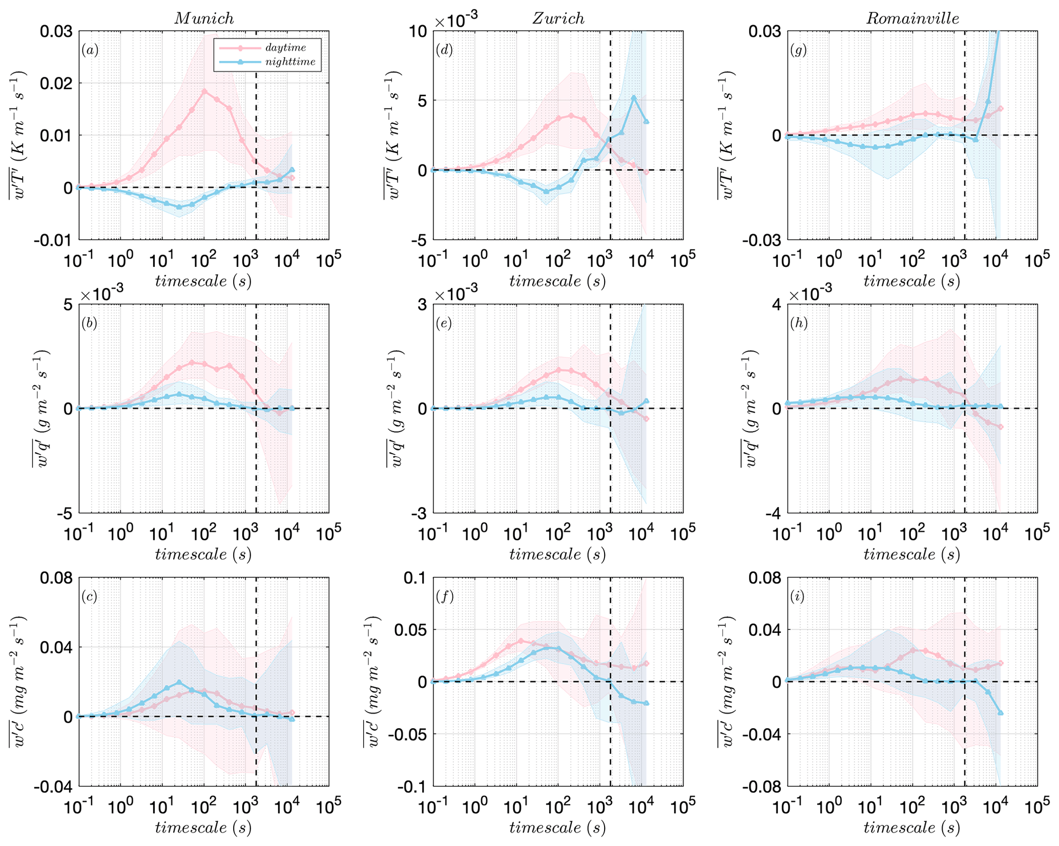
Figure 11 The 4 h multi-resolution decomposition (MRD) cospectra for fluxes of kinematic heat (a, d, g), water vapor (b, e, h), and CO₂ (c, f, i). The pink and blue lines represent the median MRD cospectra for daytime and nighttime, respectively, while the shaded area represents the corresponding interquartile range. The vertical dashed line represents the timescale of 30 min.

To further illustrate the systematic discrepancies in fluxes arising from distinct spectral loss correction schemes implemented in the three software packages, we investigated the diurnal pattern of the relative bias between fluxes computed by EddyPro (eddy4R NW) and TK3 (Fig. 10). Consistent with features observed in Fig. 8, the relative bias of fluxes computed by TK3 and EddyPro did not significantly deviate from the zero line. In contrast, fluxes computed by the eddy4R NW appeared smaller than those calculated by TK3. Notably, the most substantial difference in fluxes calculated by TK3 and eddy4R NW manifested during daytime, indicating a significant increase in daytime fluxes resulting from the low-frequency spectral correction during unstable stratification, similar to the findings from previous intercomparisons between EddyUH and EddyPro (Mammarella et al., 2016). Therefore, we conducted the multi-resolution decomposition (MRD) on scalar fluxes on a 4 h basis to further examine whether the fluxes computed using a 30 min window could capture the contributions from the large turbulent eddies (Vickers and Mahrt, 2003). As shown in Fig. 11, the nighttime MRD cospectra intersected the zero line at a timescale smaller than (or close to) 30 min, suggesting that the 30 min averaging period was sufficient to capture the low-frequency flux contributions associated with large-scale motions (Finnigan et al., 2003; Foken et al., 2012). During the daytime, however, the timescales corresponding to the MRD cospectrum crossing the zero-line exceeded 30 min. This finding indicates that fluxes contributed by turbulent eddies with timescales larger than 30 min were not effectively captured, thereby explaining the systematic differences in fluxes computed by TK3 and the eddy4R NEON workflow. This emphasizes the importance of low-frequency spectral loss correction in flux estimation for tall-tower EC systems. Importantly, NEON recognizes the challenge in applying the eddy4R NW originally designed for a median tower height of 22 m to tall-tower EC systems. It further plans to evaluate the impact of enabling eddy4R low-frequency spectral treatments for NEON towers and subsequently compare the fluxes to the counterparts estimated using a longer averaging interval albeit without low-frequency correction as commonly performed at tall towers based on Ogive analysis to determine appropriate averaging intervals. Indeed, eddy4R with low-frequency spectral treatment, storage flux, and flux mapper enabled has been shown to effectively overcome footprint bias and close the energy balance based on first principles (e.g., Metzger, 2018; Xu et al., 2020).

4 Conclusions

Through a comprehensive analysis of 5 months of tall-tower EC measurements across three European pilot cities, we conducted a comparative evaluation of friction velocity and sensible heat, latent heat, and CO₂ fluxes computed using three distinct software packages. Our investigation was designed to elucidate the sources of discrepancies in flux estimations caused by different implemented postprocessing schemes. Due to the consistency in instrumentation, raw data acquisition, and preprocessing, a very good agreement on the mean values and standard deviations was found. The comparison of the final fluxes showed a remarkable high degree of agreement among the three software packages, especially in comparison to previous software comparisons, although not yet reaching absolute perfection. The agreement on flux results was largely influenced by the distinctive spectral correction schemes implemented in each software package. Specifically, relative biases in flux estimates between TK3 and EddyPro remained below 1 % for u_∗ and around 2 % for scalar fluxes. These minor differences were predominantly caused by different analytical models employed for spectral loss correction. Conversely, systematic differences on the order of 10 % were observed for fluxes estimated by TK3 and the eddy4R NW and primarily attributed to the disabled low-frequency spectral treatment in the eddy4R NW. Our findings emphasized that flux increments resulting from low-frequency spectral loss correction were an order of magnitude larger than those stemming from high-frequency spectral loss correction. Furthermore, both the diurnal variation in relative flux biases and the MRD cospectra highlighted the crucial role of low-frequency spectral loss correction in flux estimation for tall-tower EC systems. These results constitute a valuable addition to prior software intercomparison studies (Mauder et al., 2008; Fratini and Mauder, 2014; Metzger et al., 2017) by virtue of their unique focus on urban tall-tower EC measurements. Our findings emphasize the significance of a standardized measurement setup and consistent postprocessing configurations in minimizing the systematic flux uncertainty resulting from the usage of different software packages. This approach, in turn, ensures the generation of reliable and interoperable flux estimates. We are creating an artificial dataset based on embedding perturbations from intermittent turbulence and asymmetric large eddies into the field observations. This artificial dataset will allow the quantitative evaluation of the accuracy of this scale-resolved method in flux estimation. We are currently in the process of this work and look forward to addressing these considerations comprehensively in the next paper.

Appendix A: The median diurnal cycle of the planetary boundary layer height (PBLH) at the Zurich site

Figure A1 shows the median diurnal cycle of the planetary boundary layer height (PBLH) at the Zurich site estimated from profile measurements of a collocated scanning Doppler lidar. Our observations reveal the diurnal pattern of the mixing layer, manifested as its development in the morning, peaking in the afternoon due to thermal convection while exhibiting relatively lower values during nighttime.

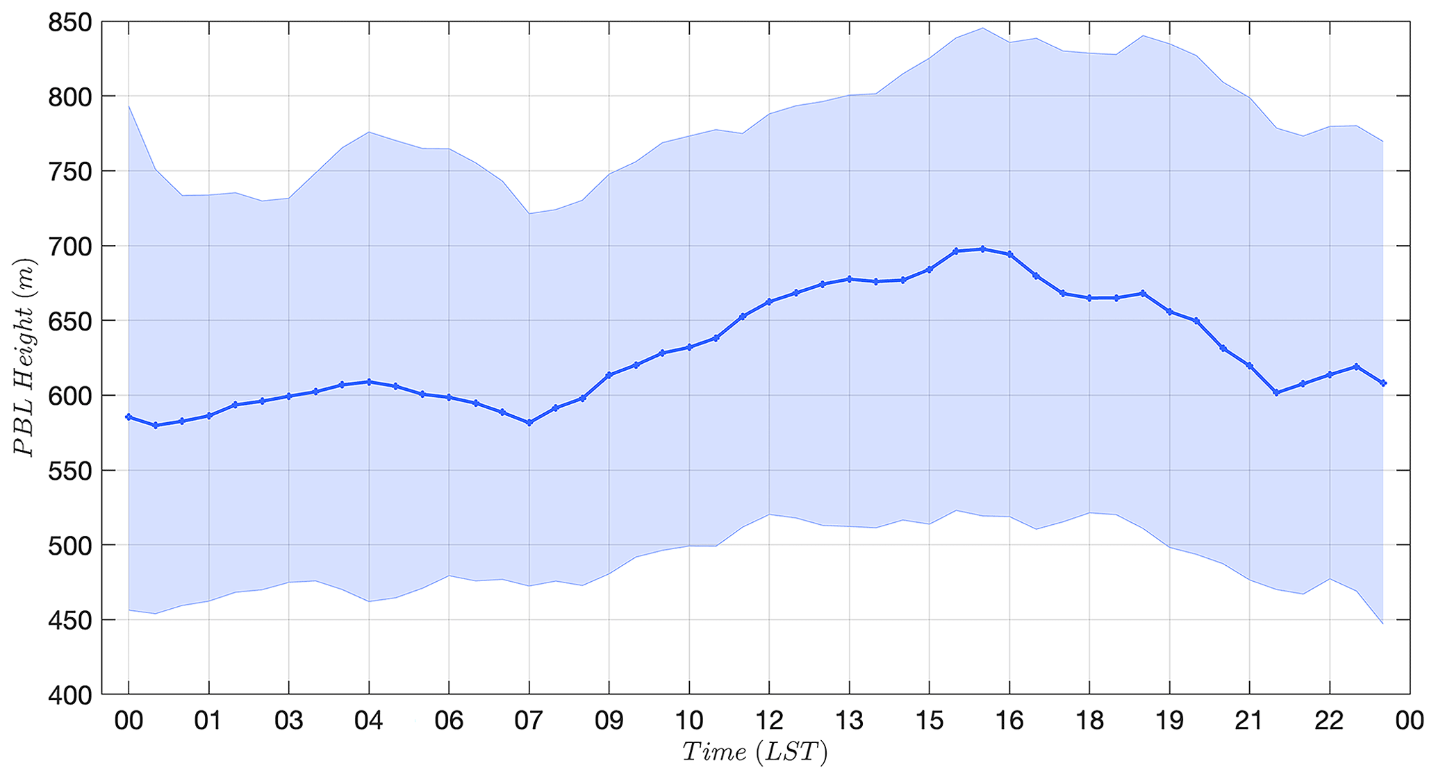
Figure A1 The median diurnal cycle of the planetary boundary layer height (PBLH) at the Zurich site estimated from profile measurements of a scanning Doppler lidar. The shaded area represents the interquartile range.

Appendix B: The distribution of relative differences in mean values, standard deviations, and fluxes estimated by EddyPro and eddy4R with respect to the counterparts estimated by TK3

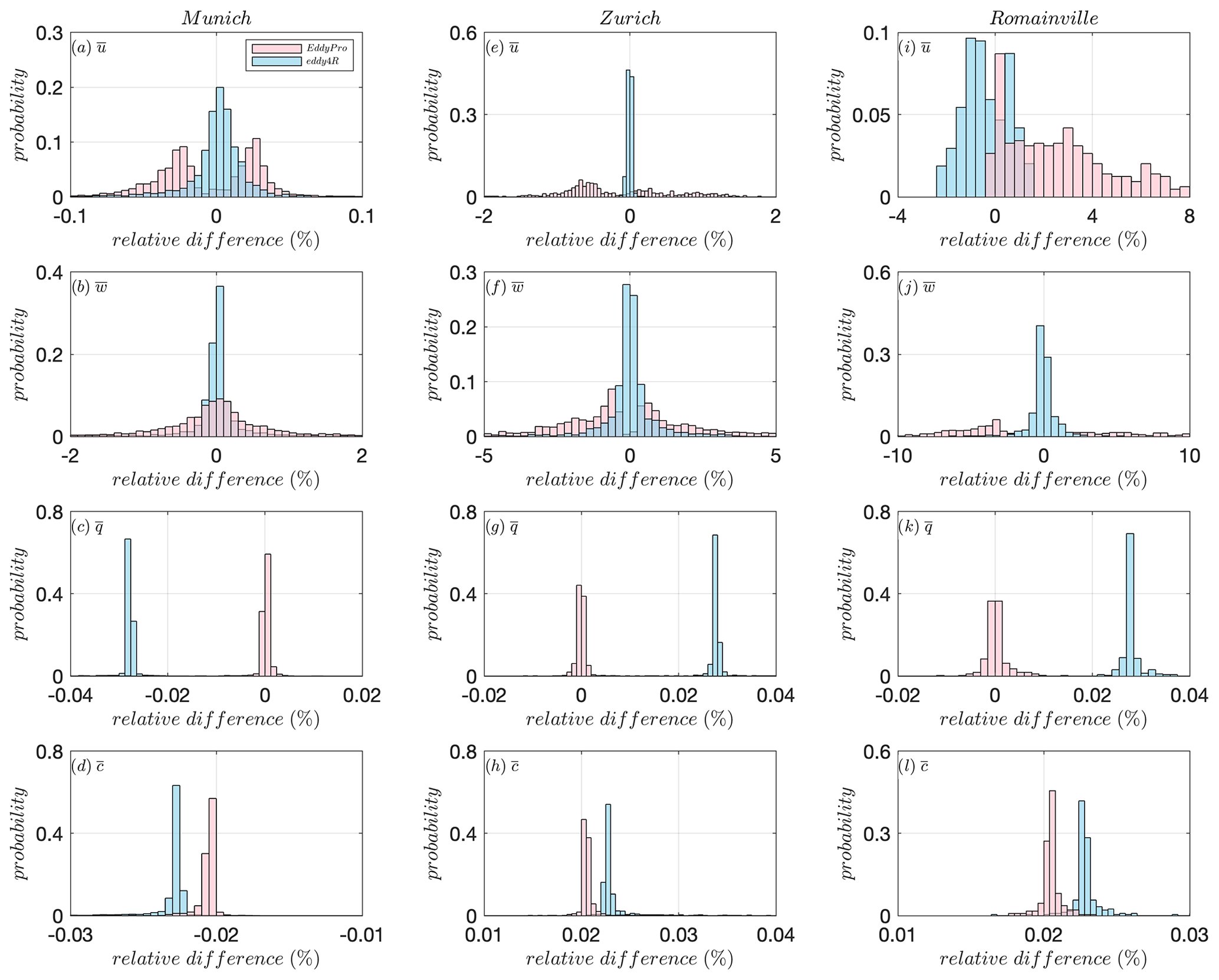
Figure B1 The distribution of the relative difference in mean values estimated by EddyPro and eddy4R with respect to the counterparts estimated by TK3.

Figure B2 The distribution of the relative difference in the standard deviations estimated by EddyPro and eddy4R with respect to the counterparts estimated by TK3.

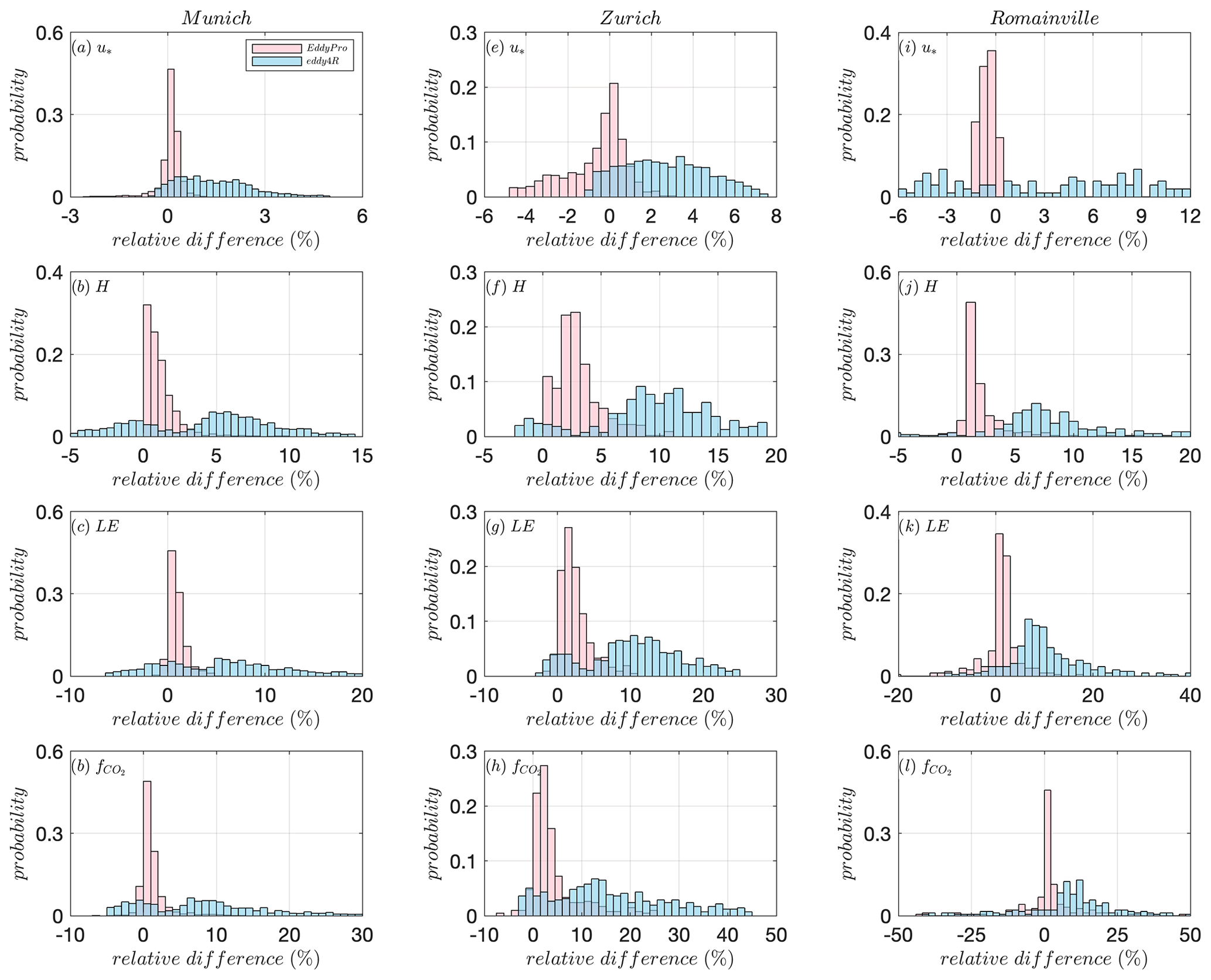
Figure B3 The distribution of the relative difference in the final fluxes estimated by EddyPro and eddy4R with respect to the counterparts estimated by TK3.