the Creative Commons Attribution 4.0 License.
the Creative Commons Attribution 4.0 License.
 | 16 May 2024
A new dual-frequency stratospheric–tropospheric and meteor radar: system description and first results
Iain Murray Reid
Bing Cai
Christian Adami
Zengmao Zhang
Mingliang Zhao
Wen Li
A new dual-frequency stratospheric–tropospheric (ST) and meteor radar has been built and installed at the Langfang Observatory in northern China. It utilizes a new two-frequency system design that allows interleaved operation at 53.8 MHz for ST mode and at 35.0 MHz for meteor mode, thus optimizing performance for both ST wind retrieval and meteor trail detection. In dedicated meteor mode, the daily meteor count rate reaches over 40 000 and allows wind estimation at finer time resolutions than the 1 h typical of most meteor radars. The root mean square uncertainty of the ST wind measurements is better than 2 m s−1 when estimating the line of best fit with radiosonde winds. Preliminary observation results for 1 month of winter gravity wave (GW) momentum fluxes in the mesosphere, lower stratosphere and troposphere are also presented. A case of waves generated by the passage of a cold front is found.
- Article
(15291 KB) - Full-text XML
- BibTeX
- EndNote


Mesosphere and stratosphere–troposphere (MST) radars operating in the VHF and UHF bands were originally hoped to provide a way of measuring winds, waves and turbulence from heights close to the ground to heights close to 100 km (see, e.g., Balsley and Gage, 1980; Chen et al., 2016; Qiao et al., 2020; Hocking, 1997, 2011). The reality was that at the most common operating frequencies near 50 MHz, these radars, no matter how powerful, could only measure winds from near the ground to heights of around 20 km during the day and night (effectively an stratospheric–tropospheric (ST) radar) and from 60 to 80 km during the day. The exception to this was for radars operating in the polar regions in the summer, where strong radar returns were also received from a range of heights between 80 and 90 km (see, e.g., Czechowsky et al., 1989; Morris et al., 2004).
Other techniques do offer a capability to measure dynamical parameters in the mesosphere and lower-thermosphere (MLT) region. These include medium-frequency partial-reflection (MFPR) radars (see Reid and Vincent, 1987; Reid, 2015) and “all-sky” meteor radars (see Hocking et al., 2001a; Holdsworth et al., 2004). MFPR radars have largely, but not completely, fallen from favor for the reasons discussed by Reid (2015), while meteor radars have become very widely applied (see, e.g., Koushik et al., 2020; Luo et al., 2021).
By combining a meteor capability within an ST radar operating at a single frequency, a radar with MST measurement capabilities can be created. This was initially applied to narrow-beam ST radars (see, e.g., Cervera and Reid, 1995; Valentic et al., 1996) and subsequently by adding an all-sky capability to an existing ST radar (see, e.g., Reid et al., 2006). The height resolution in meteor mode in the mesosphere is not as good as for a true MST radar (∼ 2 km versus ∼ 300 m), but dynamical information is typically available both day and night in the 75 to 110 km height region.
This opens the possibility of studying the dynamics of both the ST and the MLT regions with one radar. Understanding the dynamical coupling between the lower and upper parts of the atmosphere is an essential part of atmospheric dynamics. A significant contributor to coupling from below is due to the upward propagation of internal atmospheric gravity waves generated in the lower atmosphere which break in the upper atmosphere, thereby depositing momentum and energy. These wave motions can be characterized in a statistical sense by calculating the (density-normalized) Reynolds stress tensor. This contains the essential dynamical information related to both density-normalized kinetic energy, viz. , and , which represent the zonal, meridional and upward kinetic energies, and density-normalized momentum transport, viz. , and , which represent the upward transport of zonal and meridional momentum and the horizontal transport of momentum, respectively. These terms are available in the lower atmosphere (except for ) by using the five beams of the ST radar and in the upper atmosphere from the numerous radial velocities and angle of arrivals (effectively “radar beams”) of the meteor radar (Hocking, 2005). The variation in these terms with height reveals the transfer of energy and momentum from the wave motions into the background wind. For example, the divergence of the term with height is a measure of the zonal mean flow acceleration. We discuss this in more detail below.
For ST operation, a frequency near 50 MHz is typical, while for meteor operation a frequency near 30 MHz is typical. Since the meteor radar is the “add-on”, these single-frequency ST–meteor radars operate at the ST radar frequency. This is important in terms of performance, as is evident if we consider the expression for count rate given by McKinley (1961). This gives the meteor count rate N dependence on transmitted power PT, radar wavelength λ (essentially the reciprocal of the operating frequency), system gain G and received power PR as follows:
Inspection of Eq. (1) indicates that meteor counts are proportional to , so operating a meteor radar near 50 MHz results in fewer counts than for an equivalent 30 MHz radar. This is typically compensated for by the higher powers available on the ST radar, noting that counts are proportional to . Naturally, interleaving the operating modes does reduce overall meteor count rate.
There have been several single-frequency combination ST–meteor radars in operation. These include the Wakkanai ST radar (Ogawa et al., 2011; although this radar did not exercise the meteor option), the Davis ST radar (Reid et al., 2006; Holdsworth et al., 2008), the Kunming ST radar (Yi et al., 2018) and the Buckland Park ST (BPST) radar (Reid et al., 2018a). However, only the BPST radar is currently run routinely in interleaved meteor and ST mode. An obvious extension of this single-frequency approach is to operate the radar at two frequencies optimized for each operational mode. In this paper, we describe such a radar and its first results.
2.1 Overview
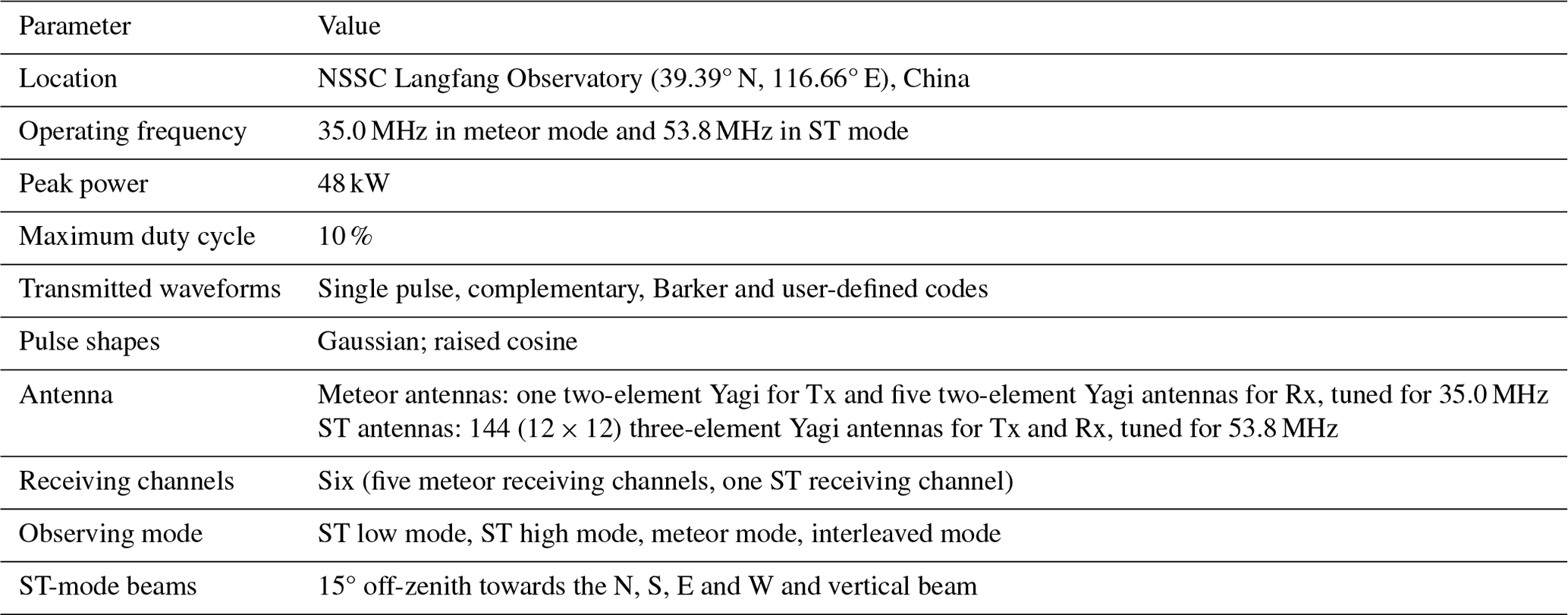
In 2010, the National Space Science Center of the Chinese Academy of Sciences (NSSC) installed an all-sky interferometric meteor radar at the Langfang Observatory (39.39° N, 116.66° E), Hebei Province (e.g., Tian et al., 2021). This radar operated at a frequency of 35.0 MHz with a peak power of 20 kW, using a vertically pointing two-element Yagi antenna and five individual two-element receiving antennas arranged as a cross-shaped interferometer, with horizontal distances of 2 or 2.5 wavelengths between antennas (the so-called “JWH configuration”; e.g., Jones et al., 1998), respectively. In cooperation with ATRAD Pty. Ltd, NSSC replaced this radar with a new combination ST–meteor radar during the period from 2018 to 2021. A unique feature of this new radar system is that two frequencies are used in interleaved operation – 53.8 MHz for ST mode and 35.0 MHz for meteor mode – thus optimizing performance for both ST wind retrieval and meteor trail detection. Table 1 summarizes the basic radar parameters.
Table 1Basic parameters of new dual-frequency ST–meteor radar.
Installation work on the new radar started in November 2018 with field site electromagnetic environment measurements. The manufacture and factory testing of all the new system modules were finished in January 2020, and the old meteor radar was switched off in April 2020. Because of COVID-19, infrastructure construction, radar module installation and system integration were delayed, with the initial radar site test completed in September 2021. Final system sign-off occurred after more than 3 months of test operation in December 2021.
2.2 System description
The two basic radar types included in this combined system have been installed at numerous locations worldwide. This includes more than 25 of the meteor radars and more than 20 of the ST radars. The basic ST radar and hardware are described in Dolman et al. (2018). The meteor radar approach is described by Holdsworth et al. (2004), noting that the power amplifiers and transceiver are rather more advanced than those described by these latter authors. The new feature of this execution is that the radar uses twelve 4 kW power amplifiers that are common to both ST and meteor operation and which operate at both 53.8 and 35.0 MHz.
The photos of the new dual-frequency ST–meteor radar are shown in Fig. 1. Outdoor antennas include the ST antenna array, meteor transmitting (Tx) antenna and receiving (Rx) array. Doppler beam steering (DBS) rack, Tx rack and Rx rack are laid from left to right in the radar hut.
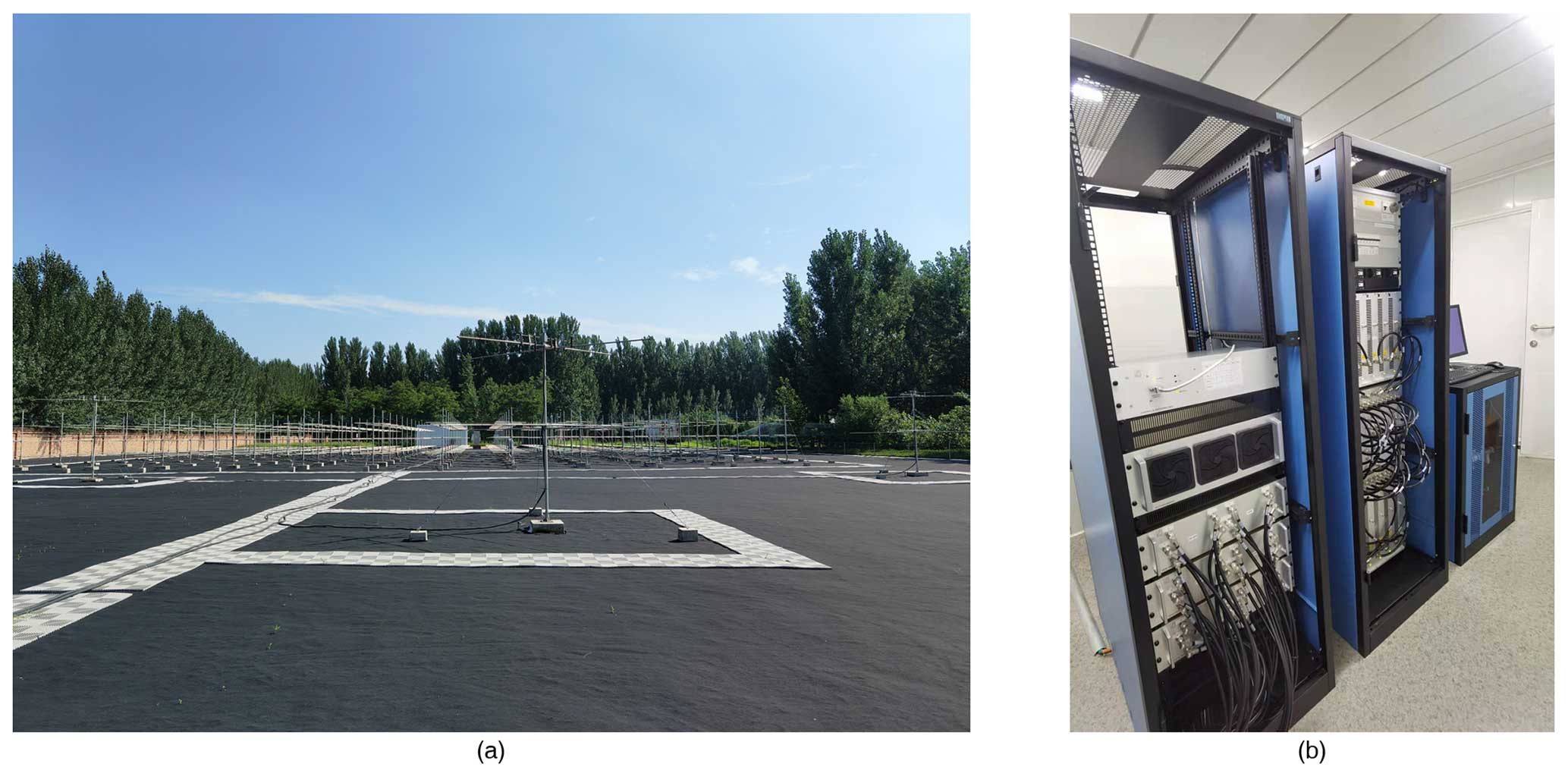
Figure 1The photos of the new dual-frequency ST–meteor radar: (a) outdoor antennas and (b) DBS rack (left), Tx rack (middle) and Rx rack (right).
The block diagram of the new dual-frequency ST–meteor radar is shown in Fig. 2. The sophisticated dual-frequency transmitter includes two sets of STX2 solid transmitters each composed of six 4 kW power amplifier (PA) modules, two sets of single-pole double-throw (SPDT) high-power (HP) relay switches, one 53.8 MHz high-power (HP) 12:2 combiner, one 53.8 MHz HP 2:1 combiner and one 35.0 MHz HP 12:2 combiner. Each PA can be operated both at 35.0 and 53.8 MHz and is connected to a SPDT HP switch. The modulated radio frequency (RF) pulse and trigger signal for the transmitter are generated by the exciter of the digital transceiver and then amplified by twelve 4 kW PA modules. Then twelve 4 kW pulses are switched to 53.8 MHz HP 12:2 combiner and then combined into a single 48 kW peak power RF output for Doppler beam steering (DBS) operation in ST mode or switched to the 35.0 MHz HP 12:2 combiner and combined into two 24 kW peak power RF outputs in meteor mode.
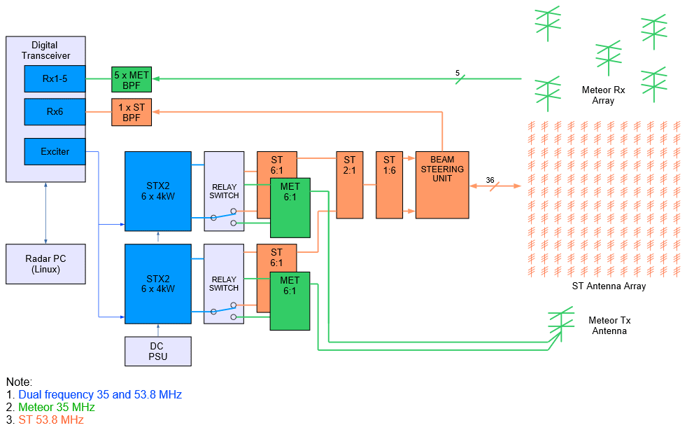
The ST antenna array consists of a square grid formed by 144 three-element linear polarized Yagi antennas and has the 3 dB full width of 6.7°. On transmission in DBS mode, switching and appropriate phase delays are used to generate a vertical beam and four off-zenith beams (north, east, south and west) with a tilt angle from the zenith of 15°. On reception, signals returned from the atmosphere are combined into one signal and fed into the digital transceiver. In meteor mode, the JWH configuration design is utilized with the entire power transmitted through a single crossed folded dipole, with half the power delivered to each arm.
A flexible six-channel digital transceiver (an exciter/receiver) is configured so that five channels are dedicated to meteor mode and one channel to ST mode. Echoes are first filtered and amplified, mixed to an intermediate-frequency (IF) band, and digitized and down-converted to baseband for further analysis.
The radar PC manages the radar and monitors system status in real time. Three operating modes are typically used: ST low mode, ST high mode and meteor mode. These are interleaved in the radar's regular configuration. In ST mode, the sampling range is usually from 300 m to 20 km. The pulse width and range sampling resolution are adjustable from 100 to 4000 m, the pulse repetition frequency (PRF) is up to 200 kHz, and three or five beams can be set to achieve different time resolutions of wind profiles from 3 min to 1 h.
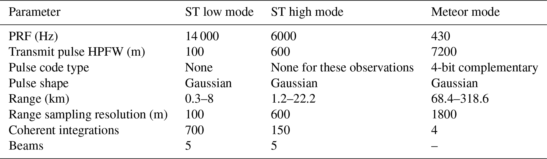
In meteor mode, the PRF is much lower at 430 Hz, allowing an unambiguous sampling range up to 300 km. The pulse width is set to no less than 1.8 km, and coded pulses are usually adopted. While the range sampling resolution remains 1.8 km, the time resolution of meteor wind profiles can be set to 15 min, 30 min and 1 h depending on the meteor count rate because of the very high count rate. The validity of these shorter averaging periods will be investigated in future work. The new radar has been operated in interleaved ST low mode, ST high mode and meteor mode since 9 November 2021, and the main operating parameters are shown in Table 2.
Table 2Operating parameters for radar observations. HPFW signifies half-power full width.
The first stage of the installation and system integration work was completed in March 2021 when a malfunction of the 53.8 MHz HP combiner was found. The damaged combiner was repaired and reinstalled in September 2021, followed by an intensive ST wind measurement test and initial data validation. A thorough system test was conducted from November to the end of December 2021, and data validation work was completed in February 2022. First results using the observational data collected from March 2021 to January 2022 are presented here to demonstrate the performance and functionality of the new radar.
3.1 Meteor radar
A good opportunity to investigate the meteor detection capability of this new radar was presented when the 53.8 MHz HP combiner was under repair. The radar was run intermittently in dedicated meteor mode (with the parameters shown in Table 2) from March to the beginning of September as the infrastructure construction continued. There were three observational periods (OPs) of dedicated meteor mode. These were 16 March to 14 April 2021, 16 to 30 June 2021 and 20 July to 7 September 2021. The first two were relatively continuous observation periods; OP3 involved several system halts, for example, from 29 July to 4 August 2021.
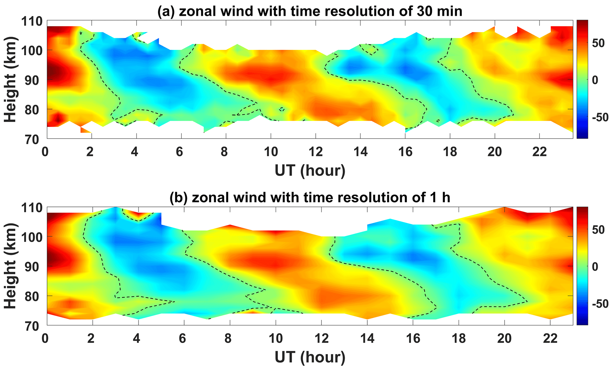
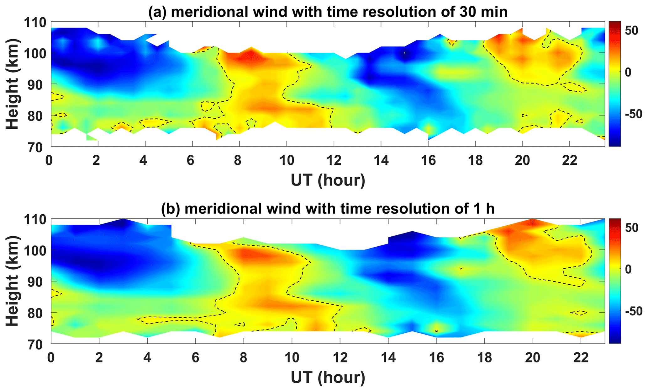
The daily meteor count rate reached over 40 000 on most complete observing days (see Fig. 3) and surpassed 60 000 (Figs. 3 and 4) at the beginning of September. Such high counts allow wind estimation of finer time resolutions (e.g., 30 min) rather than the 1 h typical of most meteor radars. Winds were calculated as described by Holdsworth et al. (2004). Representative examples of horizontal winds calculated with different time intervals are shown in Figs. 5 and 6. Inspection of these figures indicates that wind measurements between ∼ 80 and 100 km exhibit good continuity with 30 min intervals and show more detailed variations than the 1 h interval data, opening the possibility of investigating shorter-period motions such as gravity waves and turbulence.
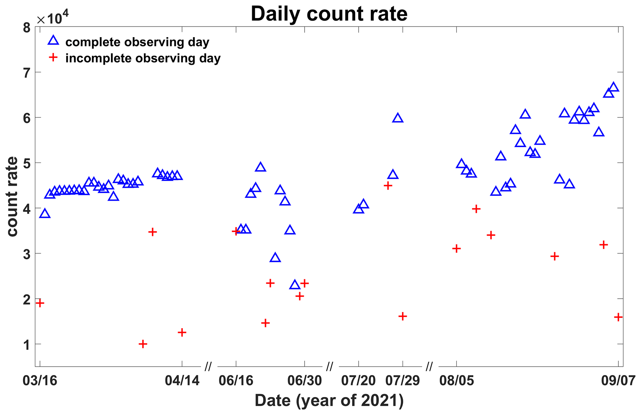
Figure 3Daily count rate during three observation periods when radar was operated in dedicated meteor mode. Count rates under 10 000 due to radar halts are not shown.
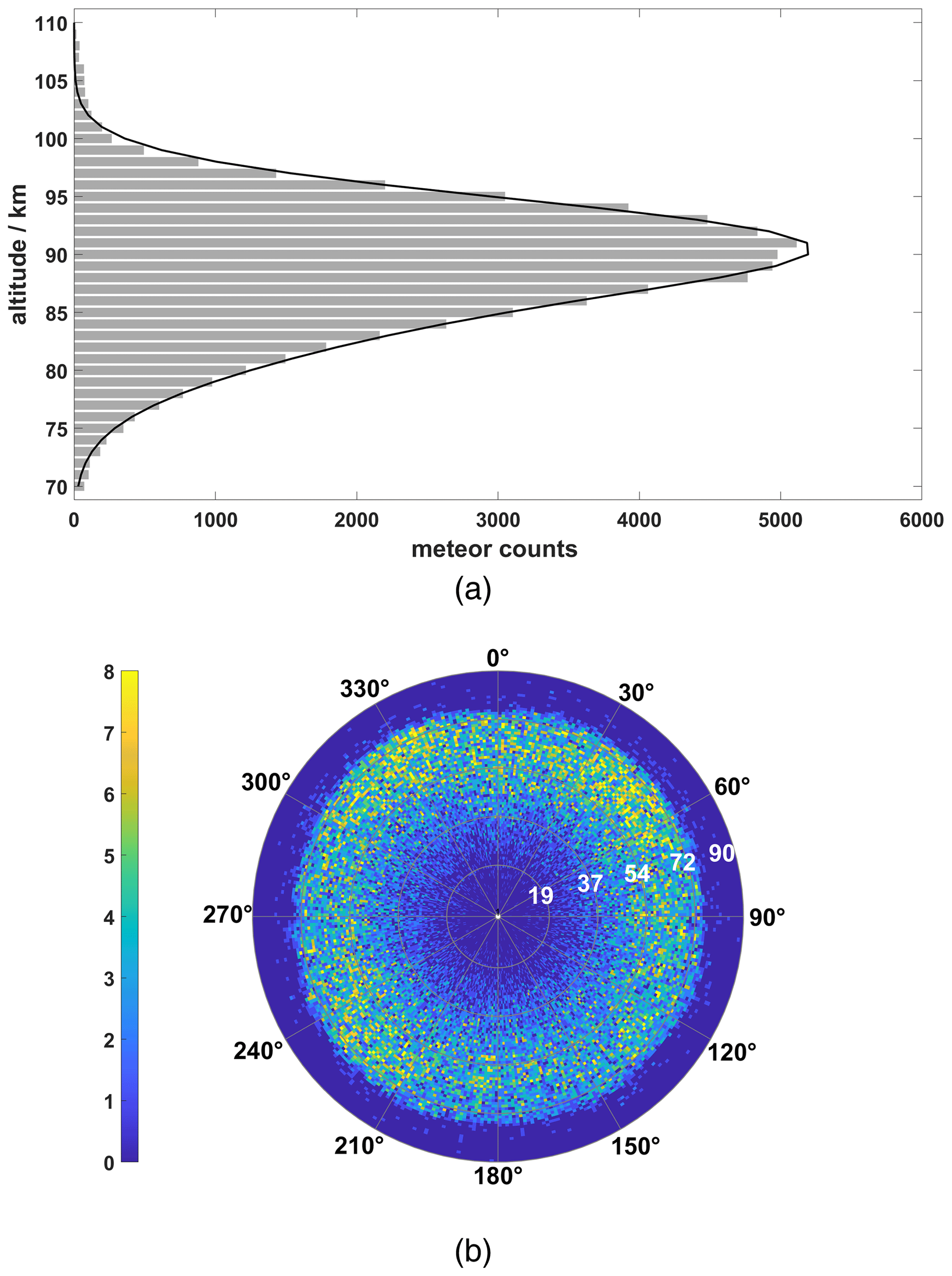
Figure 4Meteor echoes on 6 September 2021, including 66 458 underdense meteors: (a) height distribution using 1 km vertical gates and (b) azimuthal and zenithal distribution with grid of 1°.
3.2 Meteor wind comparisons
An MFPR radar has operated at the Langfang Observatory since 2009 (see, e.g., Cai et al., 2021). Notwithstanding the known bias towards wind underestimation in uncorrected MFPR winds, which is found to be up to 15 % to 40 % and strongly height dependent (see, e.g., Wilhelm et al., 2017), as well as probably being caused by any noise in the full correlation analysis (FCA), the so-called triangle size effect (TSE), low sample rate and so on (see, e.g., Reid, 2015), it is interesting to do a quick intercomparison here in anticipation of a longer future investigation. Figure 7 shows the MFPR and meteor radar winds for a height of 88 km for the 1-month period of observation. Because there are errors in each technique, the “gain factor” g0 is calculated following Hocking et al. (2001b) to account for this. In the case of the zonal wind component, this results in a slope of 0.67, so the MFPR winds are smaller than the meteor winds by about 1.49. This is similar to results found by numerous authors (see, e.g., Reid et al., 2018a) and can be used to correct the MFPR winds as the phases are consistent between the two techniques (see Fig. 8).
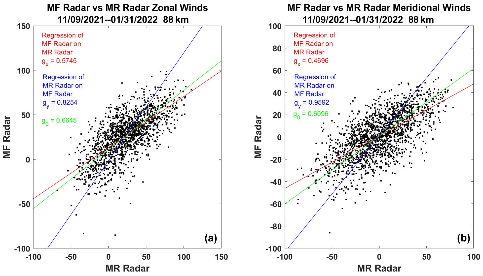
Figure 7Intercomparison of MFPR and meteor radar zonal (a) and meridional winds (b) for a height of 88 km.
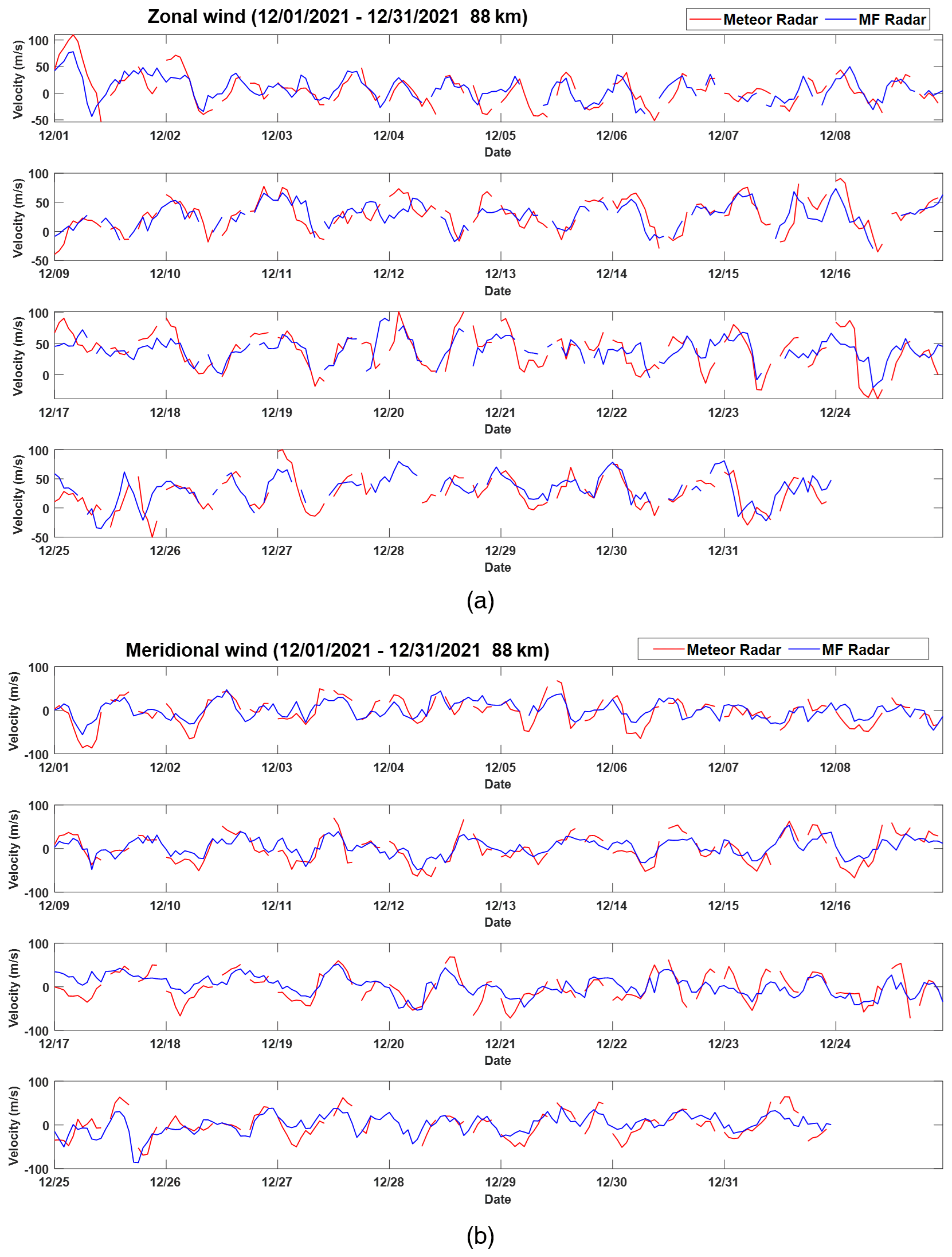
Figure 8Time series of (a) zonal and (b) meridional wind from MFPR and meteor radar for a height of 88 km.
3.3 Stratosphere–troposphere (ST) radar
On 9 November 2021, the new radar was configured for system testing and was run as follows. Interleaved five-beam ST low and high modes run from 16:30–18:10, 10:30–12:10 and 22:30–00:10 UT (matching a radiosonde launch schedule). Outside of these intervals, meteor mode ran for 20 min (10 to 30 min past the hour), and interleaved ST low and high mode ran for 40 min (30 min past the hour to 10 min past the next hour). Winds were calculated using radial velocities from five beams. The off-zenith angle of 15° is chosen to minimize the effects of aspect sensitivity on the relatively broad beams. This approach has been validated on numerous radars, including the Australian Wind Profiler Network, which incorporates four ST wind profilers of basically the same design as the present ST section of the Langfang radar (Dolman et al., 2018). This network was also used to validate Aeolus satellite results over Australia (Zuo et al., 2022).
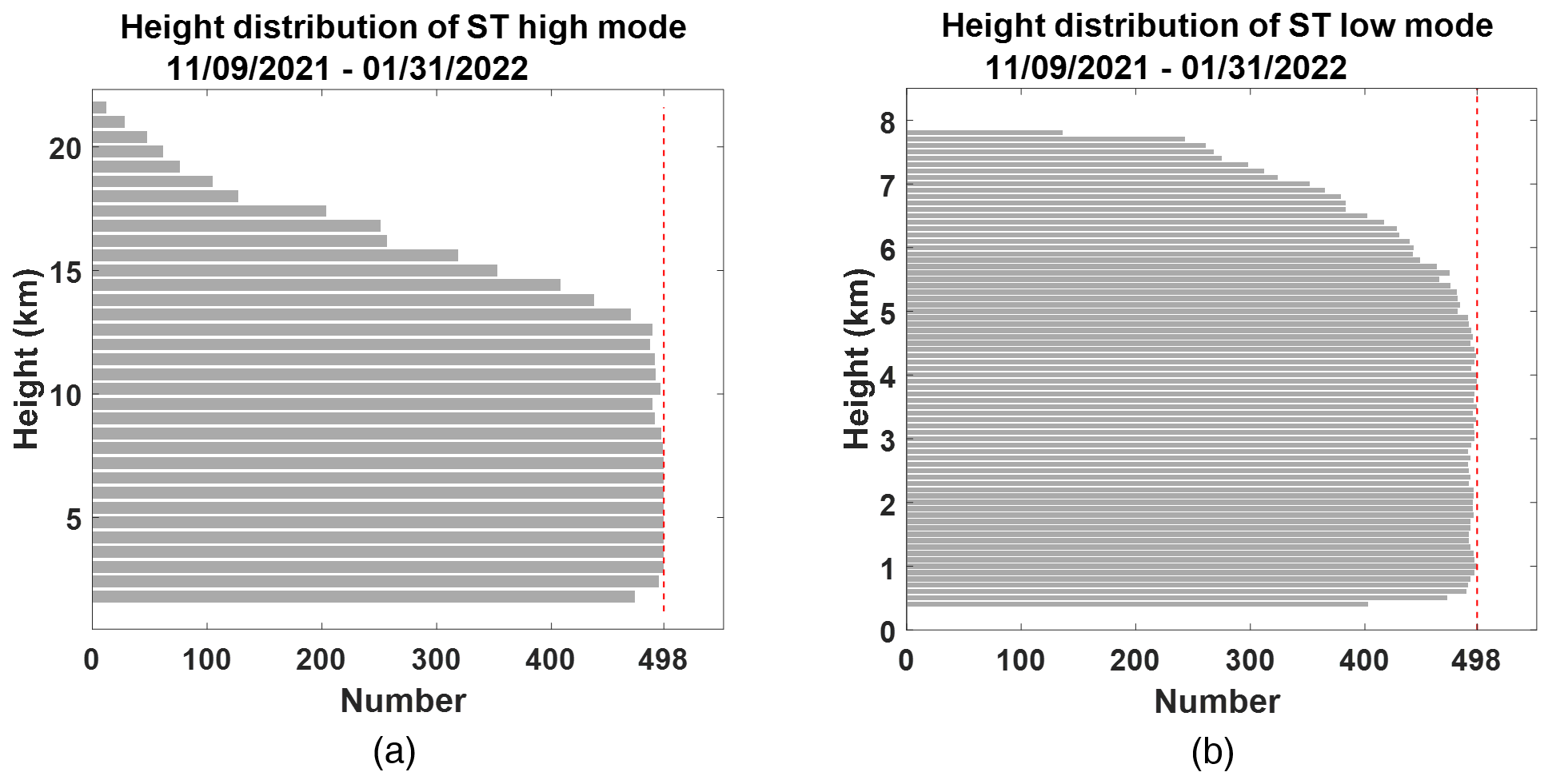
The height distributions of successful ST wind measurements for both high and low mode are shown in Fig. 9. For this observational period, 498 is the maximum profile number that could be obtained during system testing for both high and low mode. In high mode, observations begin at 1.2 km and extend to heights up to near 22 km, although there are very few of the latter. In low mode, observations begin at 300 m and extend up to heights near 8 km. For the remainder of the current work, we will focus on the high-mode observations and those heights that have acceptance rates over 50 %.
Acceptance rates for high mode for the three wind components are shown in Fig. 10a. These are about 50 % near 16 km. The mean tropopause height determined from nearby radiosonde observations is near 9.6 km and is shown in this figure as a dashed pink line. The mean winds for the entire observational period are shown in Fig. 10b, along with the standard deviation of the wind over that period.
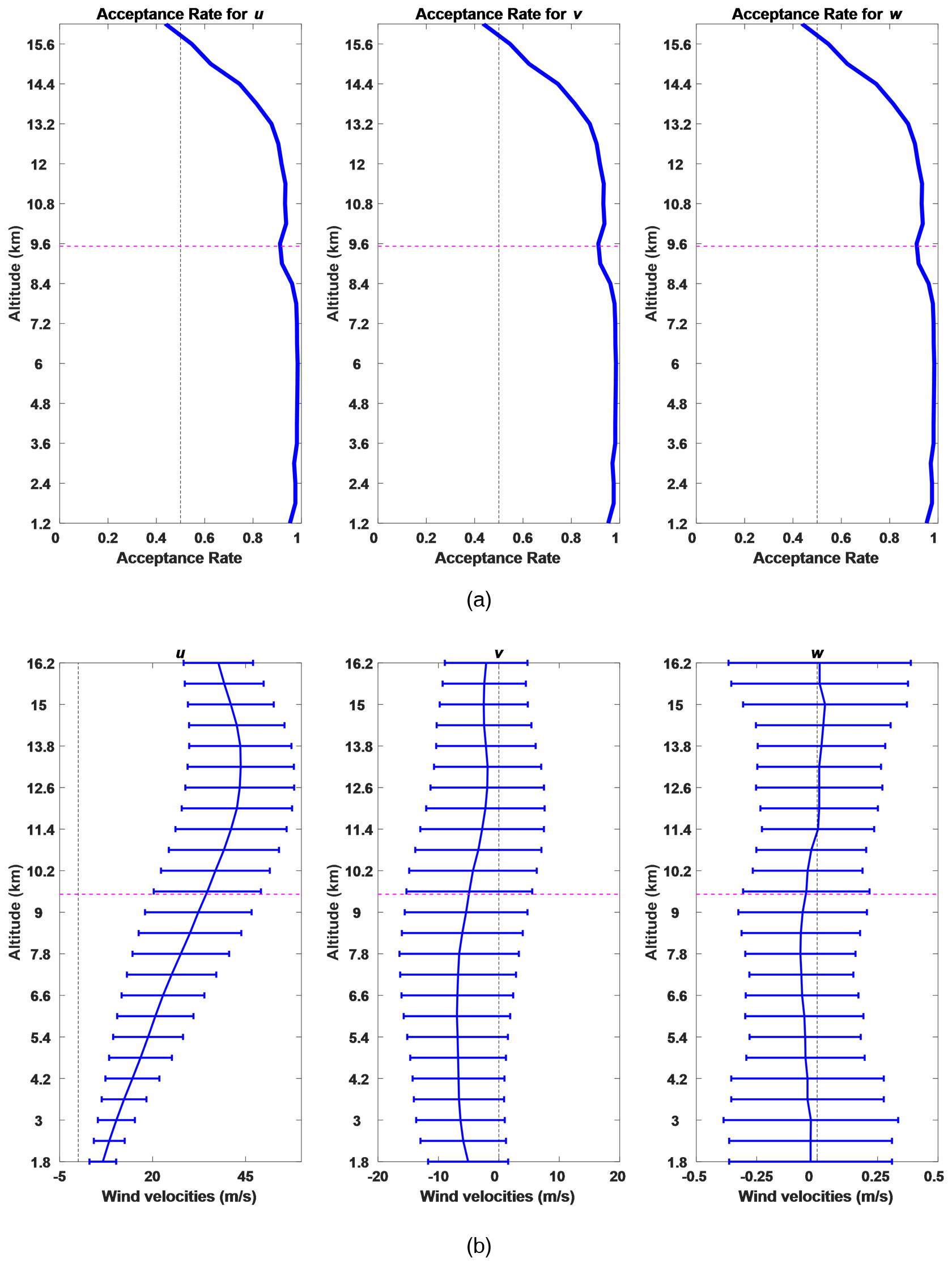
Figure 10Acceptance rates and the monthly background winds. The pink line indicates the radiosonde tropopause height. (a) The acceptance rates for the background wind estimation, which are the ratios of the number of successfully retrieved winds to the number of acquired raw data. (b) Monthly-averaged height variations in mean zonal, meridional and vertical winds along with respective standard deviation profiles.
3.3.1 ST wind comparisons
Nearly 3 months of radar observation profiles of 30 min time intervals (9 November 2021 to 31 January 2022) and radiosonde measurements was used to evaluate the reliability and accuracy of the ST wind measurements. Radiosondes are regularly launched at 11:15, 17:15 and 23:15 UT each day from the Beijing Meteorological Observatory (39.80° N, 116.47° E), station index number 54511, which is about 50 km north of the Langfang Observatory. Radiosonde data are acquired from the GTS1-type digital radiosonde, and the horizontal winds are obtained by tracking the position of the balloon using L-band radar (e.g., Li and Zhang, 2011). The raw data are sampled with 1 s interval, resulting in an uneven height resolution.
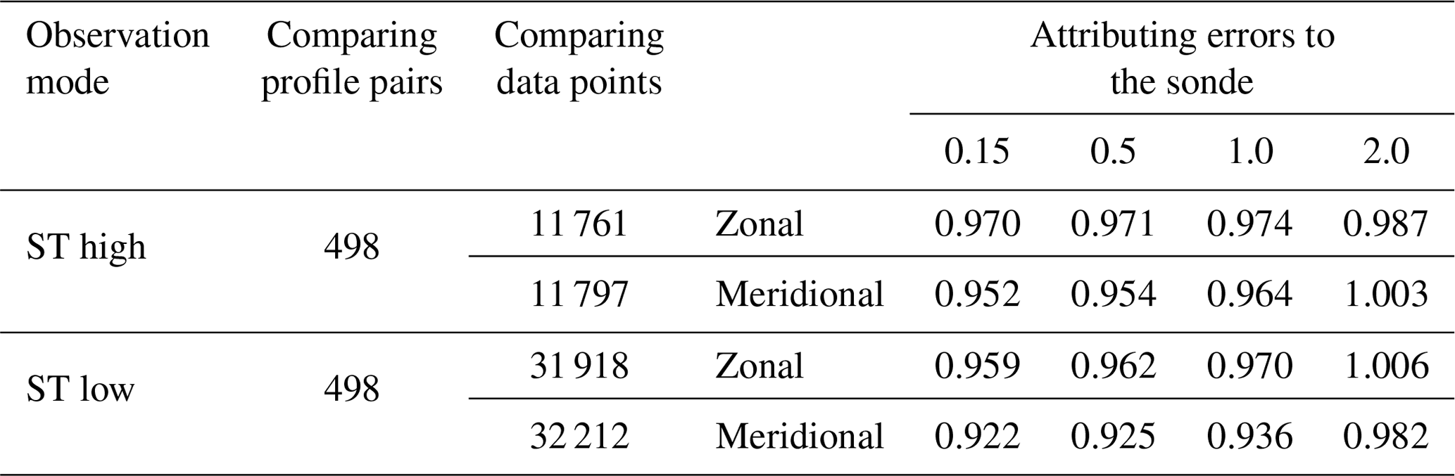
Radar profiles from 30 min before the sonde launch and 30 min after the sonde launch were selected. One sonde profile matched two (occasionally one) radar profiles and made two profile pairs. Sonde data were averaged spatially to match the radar range sampling interval in both low and high modes. Radar profiles were quality-controlled using the five-point centered moving average method (see Tian and Lü, 2017) to remove outliers mainly produced by air traffic. In addition, data corresponding to returns with signal-to-noise ratios below −12 dB were rejected. No further attempts were made to remove outliers in the radar profiles or errors in the sonde data. All available data pairs were then used to estimate the line of best fit (see Dolman et al., 2018). Comparisons for the high-mode zonal and meridional winds are shown in Fig. 11 (following the method proposed by Hocking et al., 2001b). The slopes of best-fit lines attributing root mean square (rms) errors of 0.15, 0.5, 1.0 and 2.0 to the sonde are summarized in Table 3, along with the number of profile pairs and data points.
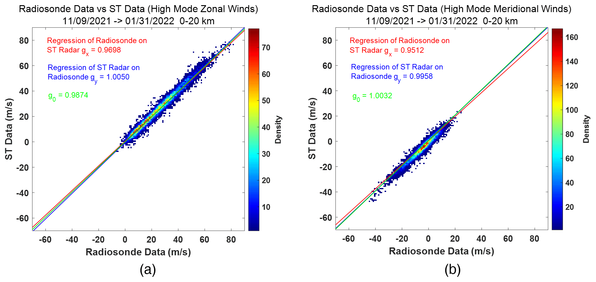
Figure 11Zonal (a) and meridional (b) colored contour wind comparisons for ST high mode. The sonde data are shown on the x axis, with radar data on the y axis, and colors indicate data density.
Table 3 demonstrates that both low and high modes are in good agreement as the slopes of best-fit lines lie within 0.98–1.01 when attributing rms errors of 2.0 m s−1 to the sonde, which might also suggest the actual uncertainty of sonde data (e.g. Dirksen et al., 2014).
Table 3The slopes of best-fit lines for zonal and meridional wind comparisons.
3.3.2 Radiosonde temperatures
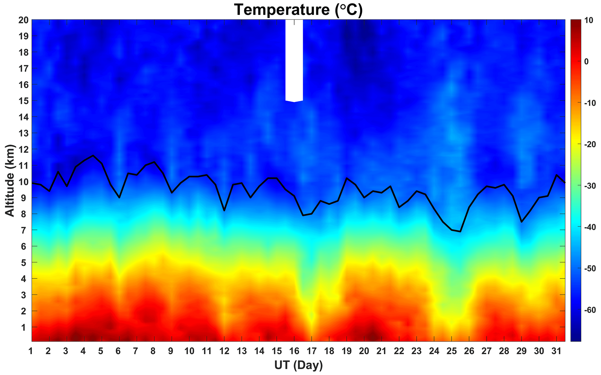
In addition to the wind velocity, the 12-hourly interval radiosonde data have been used to obtain temperature and density profiles. We note that the midnight flights only include wind data up to less than 20 km. We have estimated the tropopause height using the radiosonde data. Temperatures for the 1-month observational period and the tropopause height are shown in Fig. 12.
Gravity waves (GWs) play an important role in middle atmospheric dynamics and energetics. Most GWs are generated in the troposphere and transfer and deposit their momentum in the middle atmosphere when propagating upward. The new radar, with good height coverage and time resolution in both the lower and upper atmosphere, giving a true MST capability, permits a simultaneous investigation of the momentum transport in both regions. Here we present preliminary results of gravity wave momentum flux in the troposphere, lower stratosphere and mesosphere utilizing 1 month of radar observation data (1 to 31 December 2021). We begin with the stratospheric–tropospheric observations.
4.1 Stratospheric–tropospheric winds
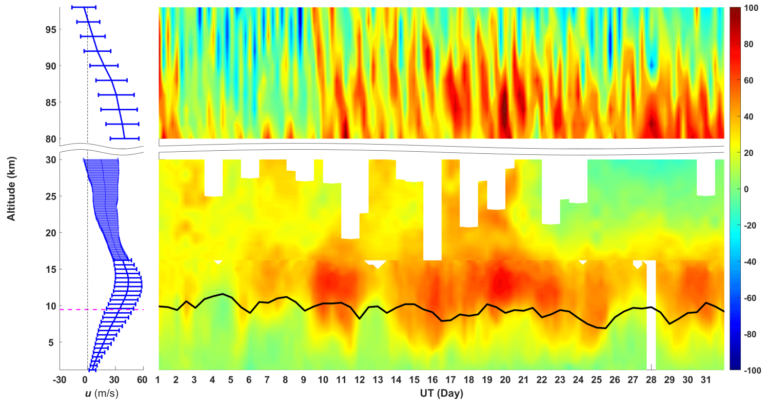
The 30 min averaged high-mode wind components for the month of observations are shown as height–time plots in Fig. 13. The five beams of line-of-sight velocities have been fitted and additional incoherent integrations were used to estimate the “raw” 3D winds, and the dwell time of each beam is about 55 s. Then “filtered” 3D winds were further obtained by five-order Butterworth high-pass filtering with a cut-off period of 18.9 h. The tropopause height has been overplotted. Zonal wind speeds are generally positive, exhibit a clear jet-like structure and reach values close to 80 m s−1 near the peak of the jet. Meridional wind speeds vary between ±50 m s−1. There are clear shorter-term variations superimposed on the longer-term wind speed variations in both the zonal and meridional wind components. Lower-tropopause temperatures are generally associated with southward winds. Vertical velocities lie in the ±1.5 m s−1 range and also show considerably shorter-period variations. These are clearer in all three wind components when periods longer than the inertial period of 18.9 h are filtered out as shown on the right-hand side of this figure. Inspection of these plots shows wave activity across the entire observational period and across all heights. Phase fronts tend to be vertical, indicating non-propagating waves, but some wave fronts are tilted, indicating upward or downward propagation. There are several periods of intense wave activity evident in both horizontal wind components. This is particularly so on 3, 5–6 and 8–9 December, especially in the filtered meridional winds and during periods of southward winds. Very strong waves are evident in both horizontal wind components with the passage of a cold front on 16 December. These extend across the tropopause but are strongest below it. This period also corresponds to the highest values of the zonal jet speed. The cold front is associated with strong southward and downward vertical winds and a temperature decline (see Figs. 12 and 13). This associated oscillation has a period of around half a day and is apparently attenuated away from the tropopause but evident over the entire height region of the observations. It continues through 17 to 20 December.
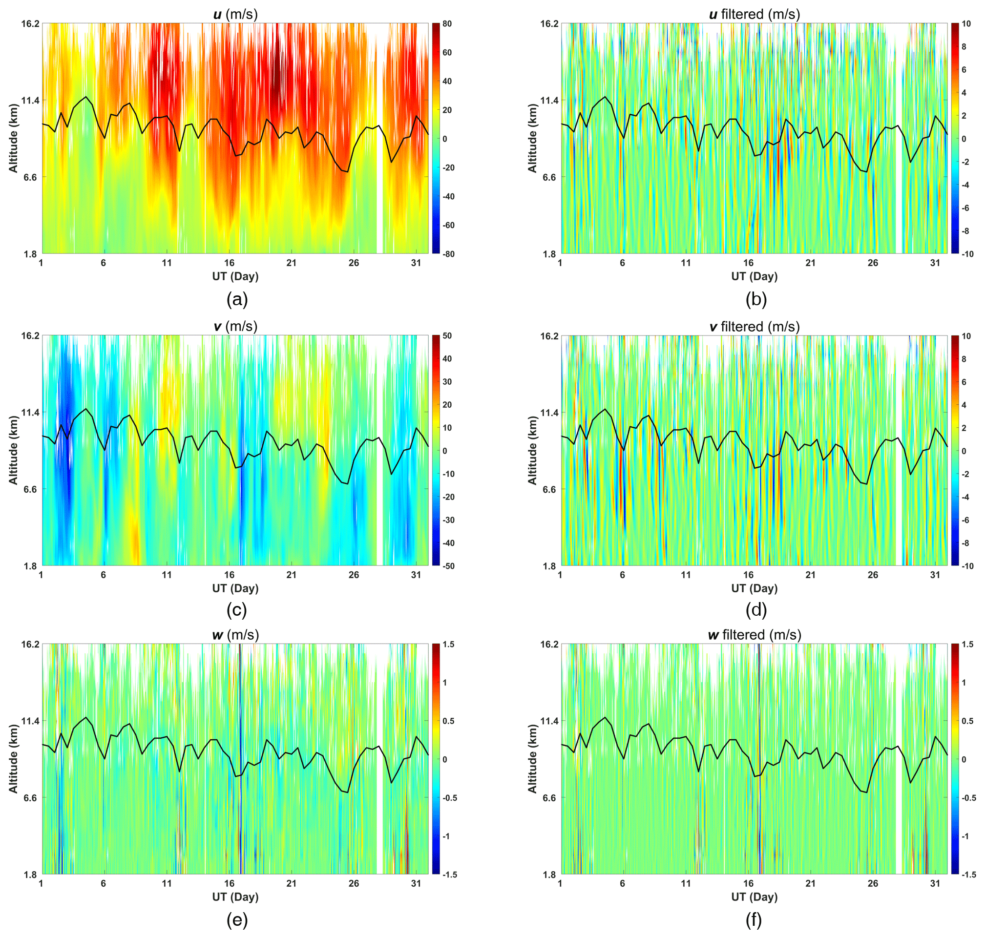
Figure 13“Raw” and “filtered” (for periods less than 18.9 h) background winds from 30 min averaged ST high-mode observation data. Black line indicates tropopause height: (a) raw zonal wind, (b) filtered zonal wind, (c) raw meridional wind, (d) filtered meridional wind, (e) raw vertical wind and (f) filtered vertical wind.
4.2 Gravity wave momentum flux and vertical transport in the troposphere–lower-stratosphere region
The dual complementary coplanar beam method (see, e.g., Vincent and Reid, 1983) is adopted to make direct measurements of gravity wave momentum flux in the troposphere and lower-stratosphere (TLS) region. The difference between the mean square fluctuating radial velocities of two symmetry beams pointing at zenith angles +θ and −θ is obtained to calculate the vertical flux of horizontal momentum. For zonal components of the momentum flux ,
A similar expression applies for the meridional component of the momentum flux. Here vE, vW, vN and vS represent the radial perturbation velocities in the east, west, north and south beams, and u′, v′ and w′ refer to the fluctuating zonal, meridional and vertical winds, respectively. θE in Eq. (2) is the effective beam direction for the off-zenith beams, which should replace the apparent off-vertical angle θA considering the influence of aspect sensitivity (Reid et al., 2018b). As we have seen above, the mean winds evaluated assuming that the apparent and effective beam angles are the same are in excellent agreement with the radiosonde measurements in the present study and with numerous other intercomparisons made with this ST radar type. However, Eqs. (2) and (3) involve differencing two like quantities to obtain a small quantity, and so we apply the beam direction corrections to these measurements to ensure valid values.
A five-beam time series of radial velocities with an equivalent sampling interval of 10 min has been used to retrieve the upward horizontal fluxes. Outliers such as aircraft echoes and ground clutter were removed by taking the mean velocity in a 3 h sliding window for each height interval and discarding values exceeding 3 standard deviations from the mean. A spline was applied to fill in missing data points. The time series of perturbation profiles then were filtered using a five-order Butterworth high-pass filter to retain oscillations with a period less than the inertial period at this latitude (18.9 h). Variances were finally calculated for the filtered time series using only values corresponding to those times when real data were obtained. Estimates of the horizontal momentum fluxes are shown in Figs. 14 and 15.
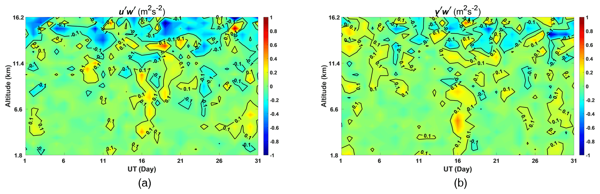
Figure 14Density-normalized momentum fluxes: (a) day-to-day variations in and (b) day-to-day variations in .
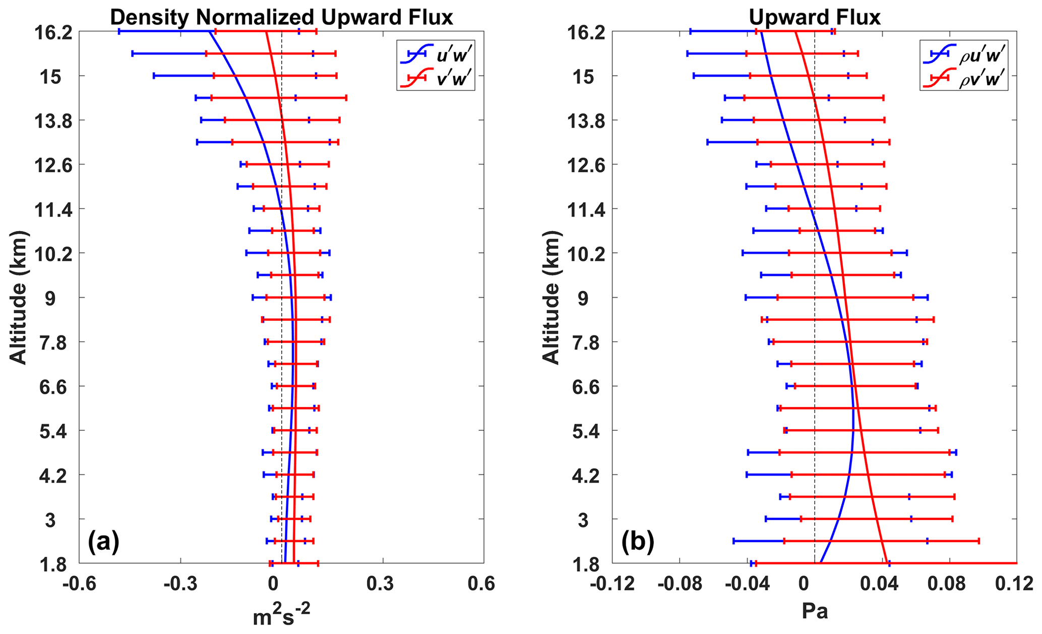
Figure 15Monthly-averaged density-normalized momentum fluxes (a) and absolute momentum fluxes (b).
From Fig. 14 we can see the cold front beginning on 16 December is associated with large values of the density-normalized fluxes. We note the strong waves evident in both the eastward and northward winds in the troposphere at this time.
Also from Fig. 14 we can see that horizontal momentum fluxes have clear day-to-day variations especially during the surface weather process. The zonal and meridional components reach values over 0.4 m2 s−2 at 4.2 and 5.4 km, respectively, on 19 December associated with a cold front (see Fig. 12) and mostly range between ±0.05 m2 s−2 in calmer weather. The mean density-normalized fluxes are shown in Fig. 15. The monthly-averaged meridional momentum fluxes are predominately northward, opposite to the mean meridional winds which are dominated by the weak southward flow. The monthly-averaged zonal momentum fluxes are near to zero in the troposphere and predominately westward when entering the stratosphere, opposite to the mean eastward flow.
We have estimated the horizontal momentum fluxes using the density derived from the radiosonde observations. Values lie in the range between ±0.5 Pa. The largest values are generally associated with the bursts of wave activity evident in Fig. 14. The mean monthly values are shown in Fig. 15. Typical values are less than 0.05 Pa.
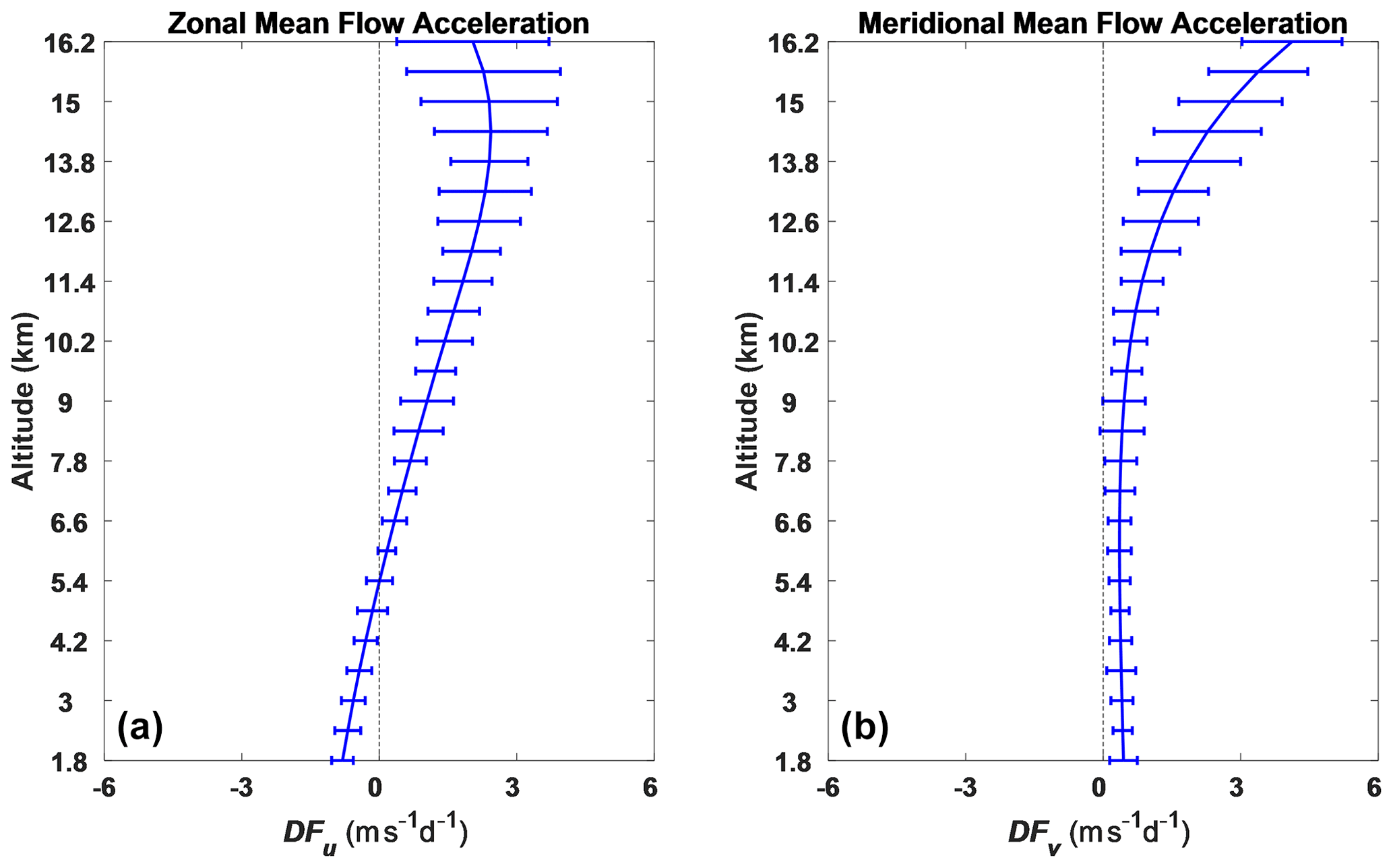
The mean monthly mean flow acceleration is calculated with Eq. (3) and is shown in Fig. 16. The mean neutral atmospheric density has been obtained from the radiosonde measurements.
Values are typically larger in the stratosphere than the troposphere. Mean values are generally less than about 3 m s−1 d−1. These values are significant and generally in agreement with previous measurements (e.g., Fritts and Alexander, 2003), but 1 month is likely too short a period given the complex dynamics of this region to infer too much from these observations. However, we do note the potential for longer periods of observations to contribute to the better understanding of the tropospheric and stratospheric dynamics over this region of China (see, e.g., Xu et al., 2023).
4.3 Mesosphere–lower-thermosphere winds
To calculate the meteor winds, 3-hourly averaged horizontal winds, stepped in hourly intervals, were determined from the measured radial velocities (Hocking et al., 2001a) using uniform altitude bins of 2 km centered on 80 to 98 km. Meteors that have zenith angles of less than 10° or more than 50°, as well as those with a radial drift velocity greater than 200 m s−1, were discarded. In order to remove outliers from the input radial-velocity distribution, the iterative scheme proposed by Holdsworth et al. (2004) was applied, which involves performing an initial fit for the wind velocities, removing the radial velocities whose value differs from the horizontally projected radial wind by more than 25 m s−1, and repeating the procedure until no outliers are found or until fewer than six meteors remain.
Two low-pass-filtered versions of the horizontal wind time series using an inverse wavelet transform with a Morlet wavelet basis were calculated by applying the method proposed by Spargo et al. (2019). A “narrow-band” low-pass wavelet filter with a cut-off of 2 d has been applied to the hourly interval horizontal winds to evaluate the mean background winds. Since a 1-month-long wind time series of each altitude was constructed for one time, a minimum scale size of 48 h and a total number of scales of 250 were selected. The raw and low-pass-filtered background horizontal winds are shown in Fig. 17. The height–time plots of Fig. 17e and f clearly include several periodicities, including a 3 to 4 d component.
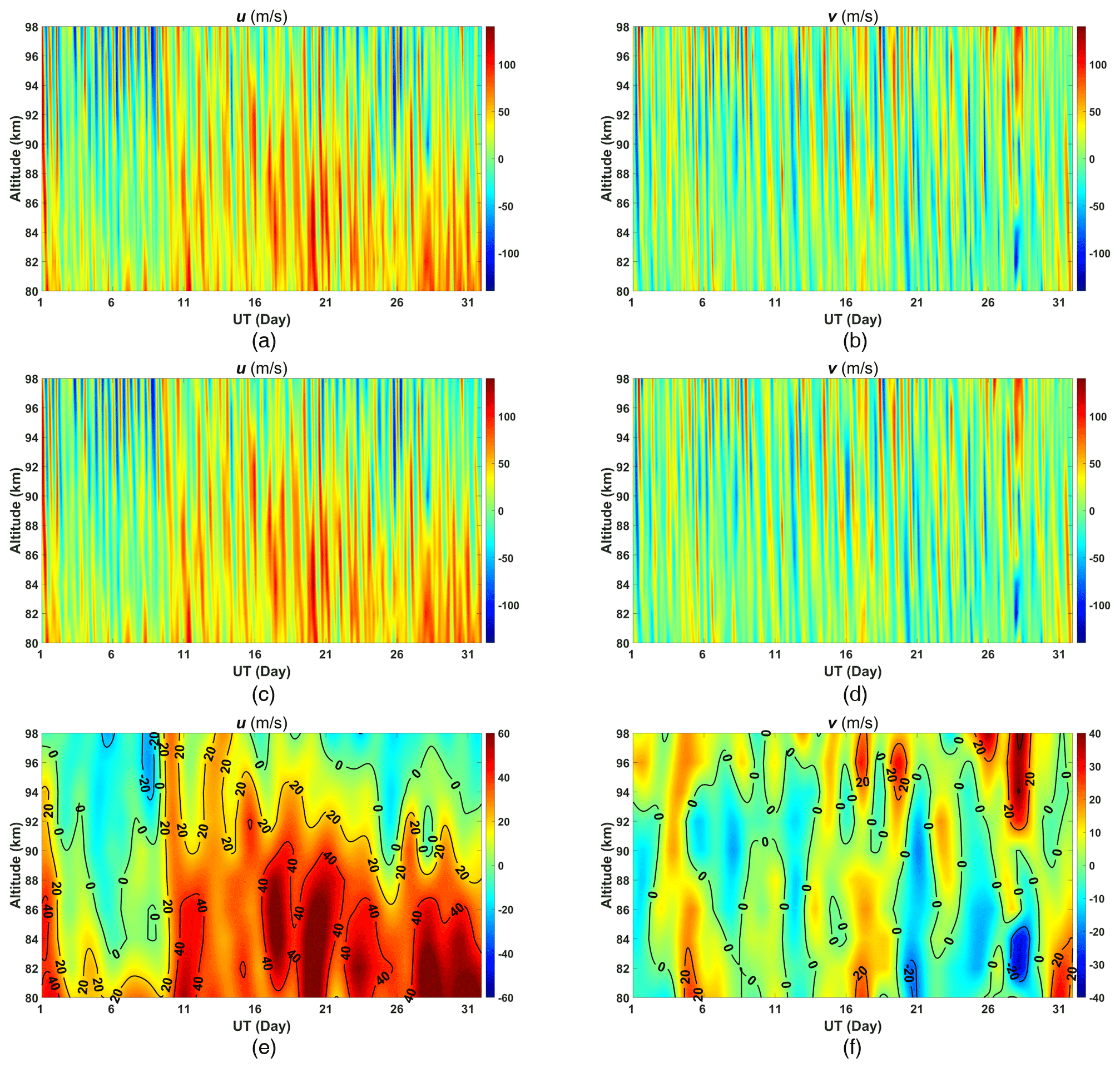
Figure 17Raw and low-pass-filtered hourly interval background horizontal winds: (a) raw zonal wind, (b) raw meridional wind, (c) broad-band low-pass-filtered zonal wind, (d) broad-band low-pass-filtered meridional wind, (e) narrow-band low-pass-filtered zonal wind and (f) narrow-band low-pass-filtered meridional wind.
The density-normalized GW momentum fluxes (, and ) and kinetic energies (, and ) in the MLT were derived following the method proposed by Hocking (2005) and subsequently improved by, e.g., Vincent et al. (2010) and Spargo et al. (2019). To remove the influence of mean winds, long-period planetary waves and tides, a “broad-band” low-pass-filtered version of the horizontal wind time series was calculated as well (see Fig. 17c and d). A 1-month wind time series of each altitude was reconstructed at one time, and a minimum scale size of 6 h and a total number of scales of 400 were selected to ensure that the filtered time series pertain to tidal-like (or longer) wind oscillations.
The reconstructed background winds were linearly interpolated between adjacent intervals to the time and height of each individual meteor echo within the given interval. The component of the value of the mean background wind along the meteor line of sight was subtracted off the individual meteor's observed radial velocity to derive the residual velocity perturbation due to GWs (see, e.g., Stober et al., 2021). Covariances were then calculated from these residual perturbation velocities using the matrix inversion method outlined in Hocking (2005). The radial-velocity outlier rejection procedure following Spargo et al. (2019) was utilized to remove meteors with dubious square radial-velocity–AOA (angle of attack) pairs from the input distribution to reduce the bias in the resulting covariance estimates. Unphysical results such as negative and and momentum flux results ( and ) with an absolute value exceeding 300 m2 s−2 were discarded as well. Covariances were evaluated with 10 d windows, with a time shift of 1 d between adjacent windows. Monthly-averaged winds and GW momentum fluxes were finally estimated.
Height–time plots of the density-normalized Reynolds stress terms are shown in Fig. 18. We note that values are typical for these parameters, but this does depend on the amount of averaging used. Shorter averaging periods than the 10 d period used here show very suggestive structures in the upward flux terms that may be related to some of the planetary wave activity evident in Fig. 17, but they are also somewhat noisy and show magnitudes that are likely much too large. We will investigate this in future work. The vertical kinetic energy and the upward fluxes of horizontal momentum fall off in value until about 86 km, where they then change little in value with height.
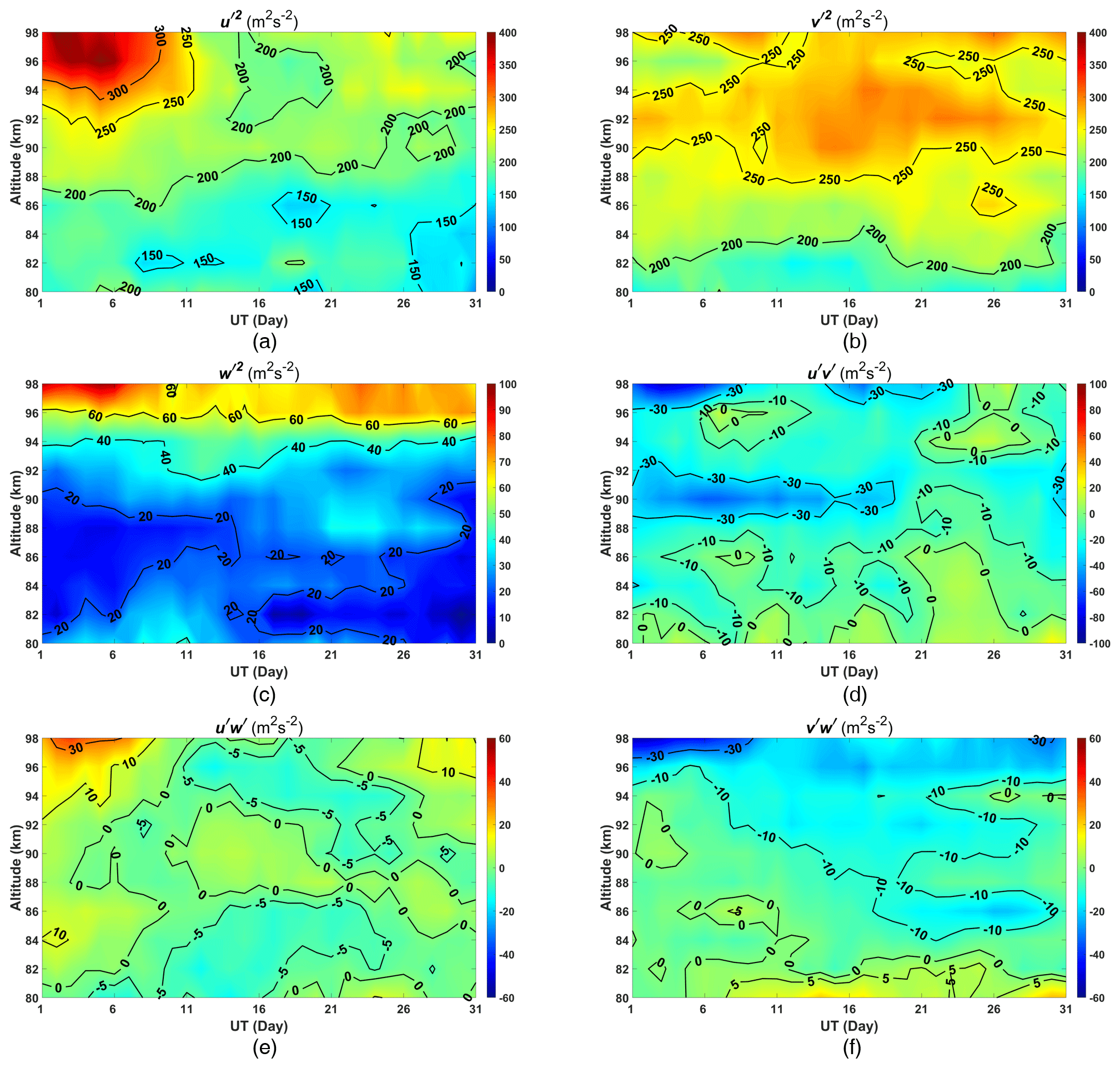
Figure 18The density-normalized Reynolds stress terms: (a) , (b) , (c) , (d) , (e) and (f) .
The monthly-averaged horizontal winds, Reynolds stress terms and mean flow acceleration are shown in Fig. 19. The mean neutral atmospheric density has been obtained from the MSIS00 atmospheric model. The horizontal kinetic energy terms decrease with increasing height, indicating the loss of wave energy with height.
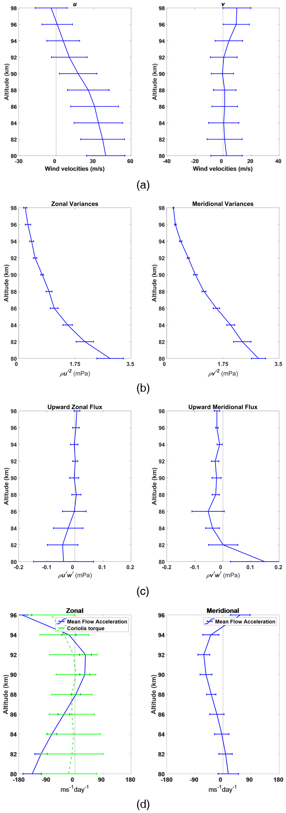
Figure 19Monthly-averaged profiles of the horizontal winds (a) and Reynolds stress terms: (b) and , (c) and , and mean flow acceleration (d).
We can see that fluxes predominantly decrease with increasing height, and monthly mean zonal winds decrease with increasing height and reverse above 96 km. The monthly-averaged meridional momentum fluxes are predominantly southward and opposite in sign to the monthly mean meridional winds which are dominated by the weak northward flow.
Mean flow accelerations were calculated with Eq. (4) and are shown as height profile time plots in Fig. 20d.
The components of the monthly-averaged mean flow acceleration are shown in Fig. 20d along with the Coriolis torque due to the local meridional wind. This has been reversed in sign for ease of comparison. Values of the mean flow acceleration are easily large enough to balance the Coriolis torque in the zonal case and have a similar form.
4.4 Integrated wind observations
The new radar provides winds in the troposphere and stratosphere and in the mesosphere and lower thermosphere, and it is interesting to consider the winds available above the radar. Figures 20 and 21 show the 6 h interval horizontal background winds of the dual-frequency ST–meteor radar covering heights from near 1 to 16 km and from 80 to near 98 km, along with 12 h interval horizontal background winds of radiosondes covering heights from 16 to 30 km. These demonstrate the true MST capability of the new radar. With the addition equipment, such as a Rayleigh Doppler lidar also built by NSSC (see, e.g., Yan et al., 2017), there is potential to fill the radar “gap” region and provide a continuous wind profile from the ground to heights near 100 km, fulfilling one of the goals of the original vision for MST radars.
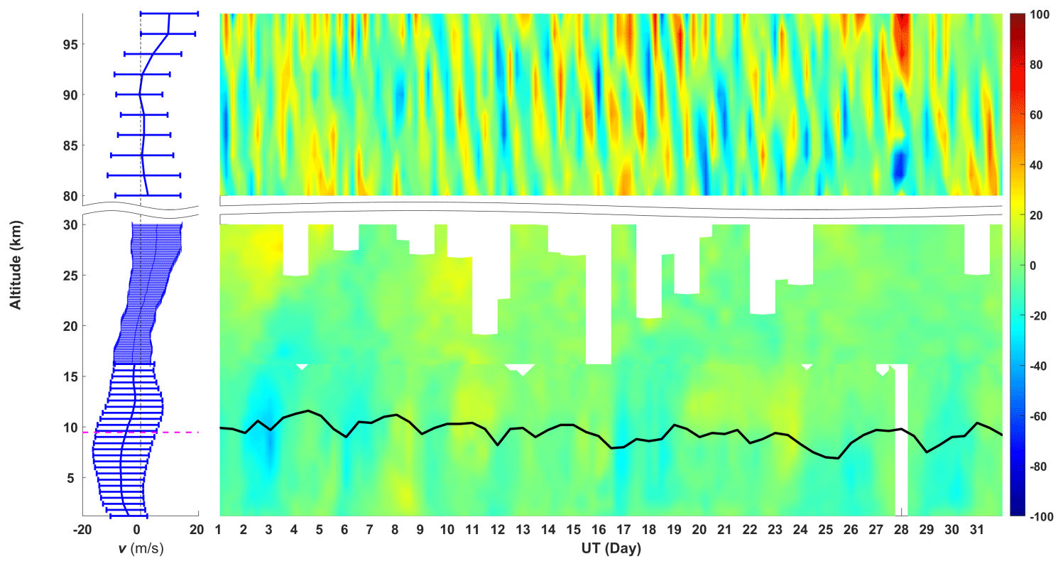
Figure 21Meridional wind. Pink line (left) and black line (right) indicate tropopause height.
The present paper gives the description of the system design and functionality of a new dual-frequency ST–meteor radar installed at the Langfang Observatory of NSSC in China. The system has been designed to provide a true measurement capability in the troposphere, stratosphere and mesosphere–lower-thermosphere region. To achieve this, two frequencies (53.8 MHz and 35.0 MHz) are used in interleaved operation to optimize performance for both ST wind retrieval and meteor trail detection, respectively. The first results clearly demonstrate that the new radar exhibits a true MST capability. In solo meteor mode, the daily meteor count rate routinely reaches over 40 000, and it has achieved daily counts exceeding 65 000. This is an excellent result and permits wind estimation at better time resolutions than the 1 h typical of most meteor radars. We have shown results with 30 min, and the radar has the potential to go to shorter time resolutions (∼ 15 min). This will enable the investigation of shorter-period motions including gravity waves in the mesosphere. The high count rates also permit a 1 km height resolution to be achieved and will also shorten the averaging times required to obtain valid estimates of the density-normalized upward fluxes of horizontal momentum and improve estimates of the other components of the Reynolds stress tensor (Spargo et al., 2019).
In ST low mode, useful winds are measured from a starting height of 500 m, and in high mode at 600 m resolution, average acceptance rates only fall to below 50 % at heights above 16 km. The is very good performance for a 48 kW peak power ST radar. Additional improvement is expected when the pulse coding capability is implemented and optimized. Data quality is excellent. The rms uncertainty of the ST wind measurements is better than 2 m s−1 when compared with radiosonde winds from launches about 50 km north of the radar site. This is comparable to the rms error when sondes are compared to sondes.
We also present preliminary observational results of typical winter GW momentum fluxes in the TLS and MLT regions above Langfang. Intense GW activity was found during the passage of a cold front, with the GWs appearing to be trapped near the tropopause.
The ability to make near-simultaneous measurements in both the troposphere–stratosphere and mesosphere–lower-thermosphere regions will facilitate investigations of coupling throughout the atmosphere. This will be supplemented in campaigns using other equipment, such as the NSSC Rayleigh Doppler lidar. Combined observations will give us wind information from close to the ground to heights near 100 km. Consequently, this radar is expected to contribute significantly to the study of atmospheric dynamics over Langfang, China.
The radar data in this study are available on request from Qingchen Xu (xqc@nssc.ac.cn).
QX was in charge of the installation and operation of the radar and carried out the data analysis. IMR contributed to the data analysis. BC contributed to the data analysis and diagram drawing. CA supervised the installation and test running of the radar. ZZ, MZ and WL contributed to the installation and test running of the radar. QX and IMR wrote the paper.
The new radar introduced in this study was designed and manufactured by ATRAD Pty. Ltd. Iain Murray Reid is the executive director of this company, and Christian Adami is the engineer of this company.
Publisher’s note: Copernicus Publications remains neutral with regard to jurisdictional claims made in the text, published maps, institutional affiliations, or any other geographical representation in this paper. While Copernicus Publications makes every effort to include appropriate place names, the final responsibility lies with the authors.
Qingchen Xu would like to thank the Beijing Meteorological Observatory for providing the radiosonde data used in this paper.
This research has been supported by the Strategic Priority Research Program of Chinese Academy of Sciences (grant no. XDA17010302); Chinese National Science Foundation (grant nos. 12241101, 42174192 and 11872128); and the Pandeng Program of National Space Science Center, Chinese Academy of Sciences.
This paper was edited by Wen Yi and reviewed by three anonymous referees.
Balsley, B. B. and Gage, K. S.: The MST radar technique: Potential for middle atmospheric studies, Pure Appl. Geophys., 118, 452–493, https://doi.org/10.1007/BF01586464, 1980.
Cai, B., Xu, Q. C., Hu, X., Cheng, X., Yang, J. F., and Li, W.: Analysis of the correlation between horizontal wind and 11-year solar activity over Langfang, China, Earth Planet. Phys., 5, 270–279, https://doi.org/10.26464/epp2021029, 2021.
Cervera, M. A. and Reid, I. M.: Comparison of simultaneous wind measurements using colocated VHF meteor radar and MF spaced antenna radar systems, Radio Sci., 30, 1245–1261, https://doi.org/10.1029/95RS00644, 1995.
Chen, G., Cui, X., Chen, F., Zhao, Z., Wang, Y., Yao, Q., Wang, C., Lü, D., Zhang, S., Zhang, X., Zhou, X., Huang, L., and Gong, W.: MST Radars of Chinese Meridian Project: System Description and Atmospheric Wind Measurement, IEEE T. Geosci. Remote, 54, 4513–4523, 2016.
Czechowsky, P., Reid, I. M., Rüster, R., and Schmidt, G.: VHF radar echoes observed in the summer and winter polar mesosphere over Andøya, Norway, J. Geophys. Res.-Atmos., 94, 5199–5217, https://doi.org/10.1029/JD094iD04p05199, 1989.
Dirksen, R. J., Sommer, M., Immler, F. J., Hurst, D. F., Kivi, R., and Vömel, H.: Reference quality upper-air measurements: GRUAN data processing for the Vaisala RS92 radiosonde, Atmos. Meas. Tech., 7, 4463–4490, https://doi.org/10.5194/amt-7-4463-2014, 2014.
Dolman, B. K., Reid, I. M., and Tingwell, C.: Stratospheric tropospheric wind profiling radars in the Australian network, Earth Planets Space, 70, 170, https://doi.org/10.1186/s40623-018-0944-z, 2018.
Fritts, D. C. and Alexander, M. J.: Gravity wave dynamics and effects in the middle atmosphere, Rev. Geophys., 41, 1003, https://doi.org/10.1029/2001RG000106, 2003.
Hocking, W. K.: Recent advances in radar instrumentation and techniques for studies of the mesosphere, stratosphere, and troposphere, Radio Sci., 32, 2241–2270, https://doi.org/10.1029/97RS02781, 1997.
Hocking, W. K.: A new approach to momentum flux determinations using SKiYMET meteor radars, Ann. Geophys., 23, 2433–2439, https://doi.org/10.5194/angeo-23-2433-2005, 2005.
Hocking, W. K.: A review of Mesosphere-Stratosphere-Troposphere (MST) radar developments and studies, circa 1997–2008, J. Atmos. Sol.-Terr. Phy., 73, 848–882, https://doi.org/10.1016/j.jastp.2010.12.009, 2011.
Hocking, W. K., Fuller, B., and Vandepeer, B.: Real-time determination of meteor-related parameters utilizing modern digital technology, J. Atmos. Sol.-Terr. Phy., 63, 155–169, https://doi.org/10.1016/S1364-6826(00)00138-3, 2001a.
Hocking, W. K., Thayaparan, T., and Franke, S. J.: Method for statistical comparison of geophysical data by multiple instruments which have differing accuracies, Adv. Space Res., 27, 1089–1098, https://doi.org/10.1016/S0273-1177(01)00143-0, 2001b.
Holdsworth, D. A., Reid, I. M., and Cervera, M. A.: Buckland Park all-sky interferometric meteor radar, Radio Sci., 39, RS5009, https://doi.org/10.1029/2003RS003014, 2004.
Holdsworth, D. A., Murphy, D. J., Reid, I. M., and Morris, R. J.: Antarctic meteor observations using the Davis MST and meteor radars, Adv. Space Res., 42, 143–154, https://doi.org/10.1016/j.asr.2007.02.037, 2008.
Jones, J., Webster, A. W., and Hocking, W. K.: An improved interferometer design for use with meteor radars, Radio Sci., 33, 55–66, https://doi.org/10.1029/97RS03050, 1998.
Koushik, N., Kumar, K. K., Ramkumar, G., Subrahmanyam, K. V., Kishore Kumar, G., Hocking, W. K., He, M., and Latteck, R.: Planetary waves in the mesosphere lower thermosphere during stratospheric sudden warming: observations using a network of meteor radars from high to equatorial latitudes, Clim. Dynam., 54, 4059–4074, https://doi.org/10.1007/s00382-020-05214-5, 2020.
Li, W. and Zhang, Y.-C.: The Wind-finding Performance Evaluation of GFE(L)1 Secondary Radar, Journal of Chengdu University of Information Technology, 26, 91–97, https://doi.org/10.16836/j.cnki.jcuit.2011.01.015, 2011.
Luo, J., Gong, Y., Ma, Z., Zhang, S., Zhou, Q., Huang, C., Huang, K., Yu, Y., and Li, G.: Study of the quasi 10-day waves in the MLT region during the 2018 February SSW by a meteor radar chain, J. Geophys. Res.-Space, 126, e2020JA028367, https://doi.org/10.1029/2020JA028367, 2021.
McKinley, D. W. R.: Meteor Science and Engineering, 1st edn., McGraw-Hill, ASIN: B0006AWT8A, 1961.
Morris, R. J., Murphy, D. J., Reid, I. M., Holdsworth, D. A., and Vincent, R. A.: First polar mesosphere summer echoes observed at Davis, Antarctica (68.6° S), Geophys. Res. Lett., 31, L16111, https://doi.org/10.1029/2004GL020352, 2004.
Ogawa, T., Kawamura, S., and Murayama, Y.: Mesosphere summer echoes observed with VHF and MF radars at Wakkanai, Japan (45.4° N), J. Atmos. Sol.-Terr. Phy., 73, 2132–2141, https://doi.org/10.1016/j.jastp.2010.12.016, 2011.
Qiao, L., Chen, G., Zhang, S., Yao, Q., Gong, W., Su, M., Chen, F., Liu, E., Zhang, W., Zeng, H., Cai, X., Song, H., Zhang, H., and Zhang, L.: Wuhan MST radar: technical features and validation of wind observations, Atmos. Meas. Tech., 13, 5697–5713, https://doi.org/10.5194/amt-13-5697-2020, 2020.
Reid, I. M.: MF and HF radar techniques for investigating the dynamics and structure of the 50 to 110 km height region: a review, Progress in Earth and Planetary Science, 2, 33, https://doi.org/10.1186/s40645-015-0060-7, 2015.
Reid, I. M. and Vincent, R. A.: Measurements of mesospheric gravity wave momentum fluxes and mean flow accelerations at Adelaide, Australia, J. Atmos. Terr. Phys., 49, 443–460, 1987.
Reid, I. M., Holdsworth, D. A., Morris, R. J., Murphy, D. J., and Vincent, R. A.: Meteor observations using the Davis mesosphere-stratosphere-troposphere radar, J. Geophys. Res., 111, A05305, https://doi.org/10.1029/2005JA011443, 2006.
Reid, I. M., McIntosh, D. L., Murphy, D. J., and Vincent, R. A.: Mesospheric radar wind comparisons at high and middle southern latitudes, Earth Planets Space, 70, 84, https://doi.org/10.1186/s40623-018-0861-1, 2018a.
Reid, I. M., Rüster, R., Czechowsky, P., and Spargo, A. J.: VHF radar measurements of momentum flux using summer polar mesopause echoes, Earth Planets Space, 70, 129, https://doi.org/10.1186/s40623-018-0902-9, 2018b.
Spargo, A. J., Reid, I. M., and MacKinnon, A. D.: Multistatic meteor radar observations of gravity-wave–tidal interaction over southern Australia, Atmos. Meas. Tech., 12, 4791–4812, https://doi.org/10.5194/amt-12-4791-2019, 2019.
Stober, G., Janches, D., Matthias, V., Fritts, D., Marino, J., Moffat-Griffin, T., Baumgarten, K., Lee, W., Murphy, D., Kim, Y. H., Mitchell, N., and Palo, S.: Seasonal evolution of winds, atmospheric tides, and Reynolds stress components in the Southern Hemisphere mesosphere–lower thermosphere in 2019, Ann. Geophys., 39, 1–29, https://doi.org/10.5194/angeo-39-1-2021, 2021.
Tian, C., Hu, X., Liu, A. Z., Yan, Z., Xu, Q., Cai, B., and Yang, J.: Diurnal and seasonal variability of short-period gravity waves at ∼ 40° N using meteor radar wind observations, Adv. Space Res., 68, 1341–1355, https://doi.org/10.1016/j.asr.2021.03.028, 2021.
Tian, Y. F. and Lü, D. R.: Comparison of Beijing MST radar and radiosonde horizontal wind measurements, Adv. Atmos. Sci., 34, 39–53, https://doi.org/10.1007/s00376-016-6129-4, 2017.
Valentic, T. A., Avery, J. P., Avery, S. K., Cervera, M. A., Elford, W. G., Vincent, R. A., and Reid, I. M.: A comparison of meteor radar systems at Buckland Park, Radio Sci., 31, 1313–1329, https://doi.org/10.1029/96RS02028, 1996.
Vincent, R. A. and Reid, I. M.: HF Doppler measurements of mesospheric momentum fluxes, J. Atmos. Sci., 40, 1321–1333, https://doi.org/10.1175/1520-0469(1983)040<1321:HDMOMG>2.0.CO;2, 1983.
Vincent, R. A., Kovalam, S., Reid, I. M., and Younger, J. P.: Gravity wave flux retrievals using meteor radars, Geophys. Res. Lett., 37, L14802, https://doi.org/10.1029/2010GL044086, 2010.
Wilhelm, S., Stober, G., and Chau, J. L.: A comparison of 11-year mesospheric and lower thermospheric winds determined by meteor and MF radar at 69° N, Ann. Geophys., 35, 893–906, https://doi.org/10.5194/angeo-35-893-2017, 2017.
Xu, X., Li, M., Zhong, S., and Wang, Y.: Impact of parameterized topographic drag on a simulated Northeast China cold vortex, J. Geophys. Res.-Atmos., 128, e2022JD037664, https://doi.org/10.1029/2022JD037664, 2023.
Yan, Z., Hu, X., Guo, W., Guo, S., Cheng, Y., Gong, Y., and Yue, J.: Development of a mobile Doppler lidar system for wind and temperature measurements at 30–70 km, J. Quant. Spectrosc. Ra., 188, 52–59, https://doi.org/10.1016/j.jqsrt.2016.04.024, 2017.
Yi, W., Xue, X., Reid, I. M., Younger, J. P., Chen, J., Chen, T., and Li, N.: Estimation of mesospheric densities at low latitudes using the Kunming meteor radar together with SABER temperatures, J. Geophys. Res.-Space, 123, 3183–3195, https://doi.org/10.1002/2017JA025059, 2018.
Zuo, H., Hasager, C. B., Karagali, I., Stoffelen, A., Marseille, G.-J., and de Kloe, J.: Evaluation of Aeolus L2B wind product with wind profiling radar measurements and numerical weather prediction model equivalents over Australia, Atmos. Meas. Tech., 15, 4107–4124, https://doi.org/10.5194/amt-15-4107-2022, 2022.