Atmospheric motion vector (AMV) error characterization and bias correction by leveraging independent lidar data: a simulation using an observing system simulation experiment (OSSE) and optical flow AMVs

Accurate estimation of global winds is crucial for various scientific and practical applications, such as global chemical transport modeling and numerical weather prediction. One valuable source of wind measurements is atmospheric motion vectors (AMVs), which play a vital role in the global observing system and numerical weather prediction models. However, errors in AMV retrievals need to be addressed before their assimilation into data assimilation systems, as they can affect the accuracy of outputs.

An assessment of the bias and uncertainty in passive-sensor AMVs can be done by comparing them with information from independent sources such as active-sensor winds. In this paper, we examine the benefit and performance of a colocation scheme using independent and sparse lidar wind observations as a dependent variable in a supervised machine learning model. We demonstrate the feasibility and performance of this approach in an observing system simulation experiment (OSSE) framework, with reference geophysical state data obtained from high-resolution Weather Research and Forecasting (WRF) model simulations of three different weather events.

Lidar wind data are typically available in only one direction, and our study demonstrates that this single component of wind in high-precision active-sensor data can be leveraged (via a machine learning algorithm to model the conditional mean) to reduce the bias in the passive-sensor winds. Further, this active-sensor wind information can be leveraged through an algorithm that models the conditional quantiles to produce stable estimates of the prediction intervals, which are helpful in the design and application of error analysis, such as quality filters.

1 Introduction

The accurate estimation of global winds is critical for various scientific and practical applications, including global chemical transport modeling and numerical weather prediction. One source of wind measurements is atmospheric motion vectors (AMVs), which are obtained through the tracking of cloud or water vapor features in satellite imagery. They play a crucial role in the global observing system, providing essential data for initializing numerical weather prediction (NWP) models; these AMVs are particularly valuable for constraining the wind field in remote Southern Hemisphere regions and over the world's oceans, where other wind observations are scarce. Obtaining global measurements of 3-dimensional winds was emphasized as an urgent need in the NASA Weather Research community workshop report (Zeng et al., 2016) and identified as a priority in the 2007 National Academy of Sciences Earth Science and Applications from Space (ESAS 2007) decadal survey and in ESAS 2017. Numerous studies have demonstrated the positive impact of AMVs on the forecast accuracy of global NWP models (Bormann and Thépaut, 2004; Velden and Bedka, 2009; Gelaro et al., 2010). Further uses include studying global CO₂ transport (Kawa et al., 2004), providing inputs for weather and climate reanalysis studies (Swail and Cox, 2000), and estimating present and future wind-power outputs (Staffell and Pfenninger, 2016). Major NWP centers now incorporate AMVs from various geostationary and polar-orbiting satellites, resulting in nearly global horizontal coverage, though vertical resolution is generally quite coarse.

Numerical weather prediction integrates atmospheric motion vectors (AMVs) through a process called data assimilation, which involves combining observations of atmospheric variables with an a priori estimate of the atmospheric state (usually generated by a short-term forecast) to derive a posterior estimate of wind fields and other atmospheric state variables. To achieve accurate results, each input source of information is weighted using an inverse error covariance matrix meant to represent the accuracy of the data. Nguyen et al. (2019) analytically proved that inaccurate error characterizations of the inputs (i.e., a priori information) can adversely affect the bias and validity of the outputs; similarly, it is important to assess and, if possible, correct for biases in AMV retrievals before their subsequent usage in data assimilation. Staffell and Pfenninger (2016), for instance, observed that NASA's MERRA and MERRA-2 wind products suffer significant spatial bias, overestimating wind output by 50 % in northwest Europe and underestimating it by 30 % in the Mediterranean, and they noted that such biases can have an adverse effect on the quality of data assimilation that ingests said data. Therefore, it is of paramount importance to assess and remove the biases inherent in AMV retrievals before their usage in subsequent analysis.

In practice, correcting the bias of an AMV retrieval requires an independent proxy for the “truth”, and previous studies assessing AMV uncertainty typically compared AMVs derived from observing system simulation experiments (OSSEs) with collocated radiosonde AMVs (Cordoba et al., 2017). Here, we propose the idea of using the independent (and sparse) lidar observations of wind as a dependent variable in a supervised machine learning model for bias correction. Following the OSSE framework of Posselt et al. (2019), we examine a proof of concept that demonstrates the feasibility and performance of a bias-correction scheme in an OSSE framework. We use as our reference (truth or NatureRun) datasets output from the Weather Research and Forecasting (WRF) model run for three different weather events (Posselt et al., 2019). The water vapor fields from these WRF model runs are processed through an optical flow algorithm (Yanovsky et al., 2024) to provide AMVs, and we similarly simulate lidar observations from the same WRF model data. Finally, we assess the ability of a bias-correction algorithm to model and correct biases (relative to the simulated lidar winds) that arise from the optical flow AMV retrieval.

Velden and Bedka (2009), along with Salonen et al. (2015), highlighted the significant impact of height assignment on the uncertainty in AMVs derived from cloud movement and sequences of infrared satellite radiance images. However, this error source is intertwined with uncertainties in the water vapor profile itself, and modeling this within the OSSE framework requires extensive knowledge and parameterization of the height-assignment error process, which is beyond the scope of this paper. As such, in this paper, we will focus on fixed-height errors in the AMV estimates and the bias corrections arising therefrom.

One challenge with pairing passive-sensor and active-sensor winds is that the latter typically observe only in one direction, along the instrument's line of sight. Therefore, a question one might ask is what sort of information a researcher might be able to obtain on the entire wind vector if, for example, lidar winds are only available at sparse locations in only the line-of-sight direction. In this paper, we search for the answer to this question in an OSSE framework, and we show that a passive sensor can benefit from coincident active sensor data through algorithms that model the expectation (bias reduction) or quantiles (uncertainty quantification).

We are not aware of a similar approach in the literature for leveraging lidar wind retrievals for the improvement of AMV retrievals, even in an OSSE context. Perhaps the closest would be Teixeira et al. (2021), which combined random forest with Gaussian mixture models to form regime-based estimates of bias and uncertainty. While this approach in principle can be used to bias-correct observations, it discretizes the bias error function into a fixed number of clusters. While this discretization is useful for understanding the geophysical regimes of the underlying atmospheric processes, it is not as efficient as a model that is purposely built for bias minimization.

The intention of this paper is not to propose that the algorithms outlined here should replace error characterization methods for all AMVs. Instead, our primary objective is to demonstrate that residual error patterns exist in AMV retrieval algorithms regardless of whether they involve traditional feature tracking or optical flow. Furthermore, through meticulous variable selection and algorithm refinement, it is feasible to curtail these biases. We also provide evidence that, in these selected scenarios, the confidence intervals predicted using the quantile random forest (Meinshausen and Ridgeway, 2006) approach exhibit a predominantly positive linear correspondence with the empirical validation standard error. This correlation is a notable and valuable characteristic that carries implications for devising indicators of AMV quality.

For the remainder of this paper, we will discuss the data sources, study regions, and the optical flow AMV retrieval algorithm in Sect. 2. In Sect. 3.1, we discuss the process of variable selection, and we discuss parameter optimization and bias-reduction performance in Sect. 3.2. We follow this treatment of bias with a discussion of modeling uncertainty via prediction intervals in Sect. 3.3. Finally, we end with some discussion of the merits of our approach and plans for further studies.

2 Data sources

The evaluation of the impact of bias correction on optical flow AMVs will be carried out in the context of an OSSE. All OSSEs share these key components: (1) a reference dataset, used as a basis for comparison – in our case, this is a NatureRun (NR), which is a high-fidelity simulation mimicking real-world conditions; (2) simulators generating synthetic observations as if they were taken from the NR (this includes radiative transfer models, retrieval system simulations, and accounting for measurement errors, and spatial and temporal aspects); and (3) a quantitative methodology to evaluate information in the candidate measurements (Posselt et al., 2022). In this section, we shall discuss our choices for these components, with emphasis on the choice of study regions, the water vapor retrieval simulations, and the algorithm for computing the AMV from the water vapor.

2.1 Study regions

For a comprehensive view of the impact of bias correction across various atmospheric scenarios, we will examine three different systems which include an extratropical cyclone, tropical convection, and a hurricane at its early and late development stages. The details of these datasets describing the storm systems are summarized in Table 1. The extratropical cyclone (ETC) reference scenario is one that developed east of the United States in the western Atlantic Ocean in late November 2006. This cyclone showcases a diverse spectrum of wind speeds, water vapor contents, and gradients, providing an extensive assessment of the AMV algorithm's error traits across a wide array of atmospheric circumstances. This specific ETC case is selected due to its thorough examination in numerous previous observational studies (Posselt et al., 2008; Crespo and Posselt, 2016).

Table 1 Overview of spatial and temporal parameters for the study scenarios.

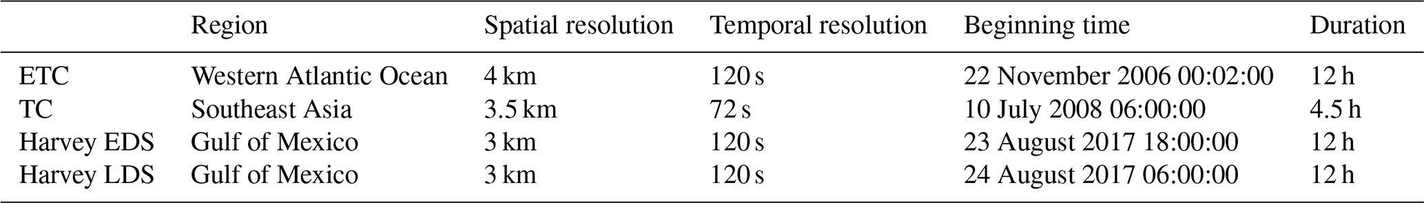
For this case, simulations are carried out using the Advanced Research Weather Research and Forecasting (WRF) Model, version 3.8.1 (Skamarock et al., 2008). The model is configured with three nested domains (d01, d02, and d03) operating at horizontal resolutions of 20, 4, and 1.33 km, respectively; although, for this paper, we will focus primarily on the data at 4 km resolution and at pressure levels of 850, 500, and 300 hPa. For our analysis, we focus primarily on the 12 h span of the storm starting on 22 November 2006 00:02:00 UTC.

For the tropical convection case, we consider a simulated water vapor dataset over the Maritime Continent from 06:00 to 10:27 UTC on 10 July 2008. Similar to the ETC scenario, we chose pressure levels of 850, 500, and 300 hPa for analysis. Further details on this simulation can be found in Yanovsky et al. (2024).

Our third study scenario is a hurricane NatureRun, produced by initializing the Weather Research and Forecasting (WRF) Model using initial conditions from an ensemble forecast of Hurricane Harvey and described in further details in Posselt et al. (2022). It consists of a free-running simulation across four two-way nested domains using version 3.9.1 of the WRF model. The initiation of this simulation occurs at 00:00 UTC on 23 August 2017, utilizing the initial state that generated the third most powerful member within an ensemble forecast of Hurricane Harvey. The ensemble's initial conditions were established through the assimilation of a conventional set of observations and all-sky satellite brightness temperatures. The NR simulation spans 5 d, ending at 00:00 UTC on 28 August 2017, while the outermost domain's boundaries are guided by analysis fields from the fifth-generation European Centre for Medium-Range Weather Forecasts (ECMWF) reanalysis (ERA5).

This simulation is notably realistic, capturing both wind patterns and humidity levels. Posselt et al. (2022) noted that it exhibits rapid intensification; within a span of 24 h, from 12:00 UTC on 24 August to 12:00 UTC on 25 August, the minimum sea level pressure plunges by approximately 40 hPa and the storm's strength escalates from category 1 to category 4. To get a view of different stages of Hurricane Harvey, we focus on two 12 h subsets of the storm: one between 18:00 UTC on 23 August and 06:00 UTC on 24 August (early development stage; Harvey EDS), and one between 06:00 UTC on 24 August and 18:00 UTC on 24 August (late development stage; Harvey LDS). Note that with the division of Harvey into early and late development stages, we have a set of four scenarios – ETC, TC, and Harvey EDS and LDS – on which we shall focus our analysis.

Traditional AMVs from cloud tracking are typically focused on high-level clouds (at around 200 hPa) and low-level clouds (at around 850 hPa). Tracking mid-level clouds poses a challenge because they are often obscured by high-level clouds. In this OSSE study, we are considering using AMVs derived from sounder-based water vapor retrievals, which are most reliable in the middle troposphere. Furthermore, lidar winds, primarily derived from the UV (Rayleigh scattering) channel, provide retrievals mainly in the middle to upper troposphere where the scattering signal is adequate for returning Doppler information, and the view is less likely to be obstructed by clouds. For these reasons, we opted to perform our OSSE error characterization experiments at the 850, 500, and 300 hPa pressure levels.

2.2 Optical flow AMVs

Optical flow methods are powerful computational techniques for analyzing the motion between two consecutive images across various fields (Horn and Schunck, 1981; Zach et al., 2007; Wedel et al., 2009). In the context of atmospheric science, these methodologies offer a sophisticated approach to extracting detailed atmospheric motion vectors (AMVs) from sequential satellite imagery, providing critical insight into wind patterns and dynamics essential for improving weather prediction models and climate research.

In Yanovsky et al. (2024), the authors employed a robust and efficient variational dense optical flow method that utilizes the conservation of pixel brightness across a pair of images, with a regularization constraint. Given a pair of images $I_{\mathrm{1}}\left(\widehat{x}\right)$ and $I_{\mathrm{2}}\left(\widehat{x}\right)$, where $\widehat{x}$ represents the pixel coordinates in the image plane, and if $\widehat{w}=(u,v)$ denotes the velocity vector field describing the apparent motion between the images, the functional being minimized with respect to $\widehat{w}$ is conceptually defined as

$$\begin{array}{}\text{(1)}& F\left(\widehat{w}\right)=\mathit{\lambda }\underset{\mathrm{\Omega }}{\int }\left|I_{\mathrm{2}}\right(\widehat{x}+\widehat{w})-I_{\mathrm{1}}(\widehat{x}\left)\right|\mathrm{d}\widehat{x}+\underset{\mathrm{\Omega }}{\int }\left(\right|\mathrm{\nabla }u|+|\mathrm{\nabla }v\left|\right)\mathrm{d}\widehat{x},\end{array}$$

where λ is the weighting parameter. The first term in $F\left(\widehat{w}\right)$ corresponds to the data fidelity term as an L1 norm between the first image and the warped second image, ensuring the similarity using the estimated motion field, $\widehat{w}$. The second term, involving the gradients of the velocity components, u and v, represents the total variation (TV) regularization term that encourages smoothness in the estimated motion field.

In order to make the problem solvable, the L1 fidelity term is linearized, enabling efficient optimization. The TV regularization term is convexified to ensure that the optimization formulation is well behaved, enabling the use of efficient numerical methods for finding the solution. To address the challenges posed by large displacements, the method employs a pyramid scheme, which processes the images at multiple scales, from coarse to fine, gradually refining the motion estimation. This multi-scale approach enhances the method’s robustness to initial estimates and increases its ability to capture a wide range of motion magnitudes. The method, referred to as the TV-L1 optical flow algorithm, effectively handles discontinuities in the flow field while preserving edges in the motion, making it particularly suitable for capturing complex motion patterns in atmospheric data or other dynamic scenes. Hence, the method balances between adhering closely to the data and ensuring a physically plausible flow field.

In our effort to obtain accurate AMVs, we applied the TV-L1 dense optical flow algorithm to four distinct simulated NatureRun datasets. These datasets represented ETC, TC, and both the early and late stages of Hurricane Harvey. The analysis in Yanovsky et al. (2024) revealed that the optical flow method had a distinct advantage over the traditional feature matching technique.

For every pair of images, the optical flow algorithm generated atmospheric motion vectors for every pixel. On the other hand, the feature matching algorithm had its limitations – it was unable to generate AMVs in specific areas, particularly near domain boundaries. Although the optical flow approach did not perfectly capture the strong winds around the hurricane with absolute precision, the flow fields it produced closely resembled the wind fields observed in the natural runs datasets. A notable metric, the root mean square vector difference (RMSVD), indicated that the errors associated with the optical flow algorithm were significantly reduced compared to those obtained with the feature matching algorithm. This resulted in an average accuracy improvement of about 30 % to 50 % for the four datasets analyzed.

An important quality of the optical flow was its robustness. The results it produced remained relatively consistent, irrespective of the time interval. This was not the case with the feature matching method, whose results showed a significant change based on time intervals (Yanovsky et al., 2024). Given these advantages, we favor the optical flow as the preferred algorithm for retrieving AMVs in this OSSE exercise.

In Fig. 1, we display the quiver plots of the wind vectors from optical flow (left column) and NatureRun (middle column) scenarios. The time stamp is chosen as the middle of the model run for each study scenario. The differences between the two wind fields (optical flow and NatureRun) are displayed in the right column of Fig. 1. We observe that the wind differences show a consistent pattern influenced by complex local factors, further complicated by what appears to be random variability and potential covariates such as wind rotation or water vapor gradients. Given our objective to model these error characteristics, we approach the problem by first considering the space of predictor variables, which is often referred to as feature selection or variable selection.

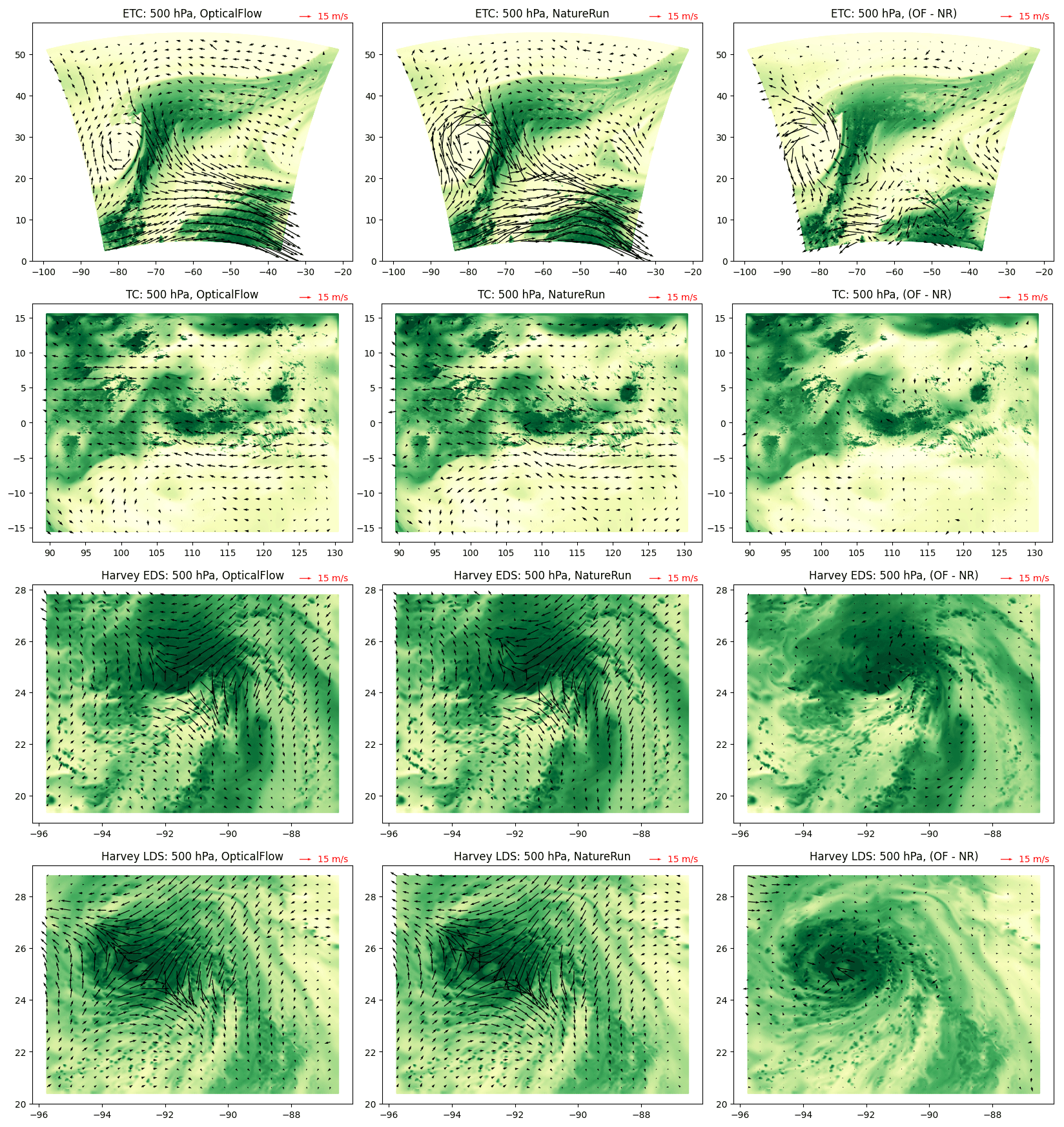
Figure 1 Quiver plots of the optical flow wind (left column), NatureRun wind (middle column), and differences (right column). The quivers are overlaid over a yellow–green heatmap of the water vapor, where yellow corresponds to low water vapor and green corresponds to high water vapor. The rows correspond to ETC, TC, Harvey EDS, and Harvey LDS. These plots are selected from the middle of each study scenario, and their UTC time stamps are 22 November 2006 06:12:00 (ETC), 10 July 2008 08:18:00 (TC), 24 August 2017 00:10:00 (Harvey EDS), and 24 August 2017 12:10:00 (Harvey LDS).

3 Modeling approach

3.1 Variable selection

Before assessing the benefits of colocating passive and active wind data, we need focus on the issue of variable selection, which involves the identification of important variables or features for predicting the target quantity. In this context, our target is the bias between retrieved AMVs and actual wind values. This selection process holds significance due to its potential to trim down the input parameter space. This reduction not only speeds up the training process but also enhances the model's reliability when dealing with unfamiliar data. Additionally, it contributes to simplifying the interpretation of model parameters.

Lidar instruments typically observe only one component of winds. Aeolus, for instance, measures “[the] component of the wind vector along the instrument's [horizontal] line of sight [HLOS]” (Lux et al., 2020). Here, we similarly assume that the active instrument in our OSSE study also observes only one component of the wind vector, though we simplify the geometry by assuming that simulated observable is the u wind. This assumption is fairly benign since it is simply a change in basis from the wind vector given by the HLOS wind and its (unobserved) perpendicular component to the much simpler (u,v) basis.

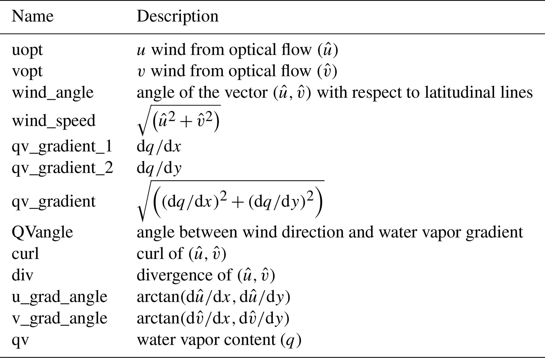
Since we wish to model the bias between the optical flow $\widehat{u}$ and the lidar u, we define the response variable as $y=\widehat{u}-u$. As for the predictor variables, Posselt et al. (2019) examined the relationship between “tracked” and “true” wind using an OSSE framework for the same ETC region as this study, and they noted that there is considerable heteroskedasticity (i.e., non-constant variance) in the wind speed difference (i.e., the tracked wind speed minus true wind speed) as a function of the water vapor, wind speed, water vapor gradient, and angle between wind direction and water vapor gradient (Fig. 6 of Posselt et al., 2019). Therefore, we start our list of potential variables with these four parameters. Since wind speed is simply a magnitude of the wind vector, $(\widehat{u},\widehat{v})$, in polar coordinates, we added the other component – wind angle – as well.

Further, we take advantage of the smooth output space of the optical flow algorithm to compute the first derivatives of $(\widehat{u},\widehat{v})$, giving rise to a 4-dimensional vector, $(\mathrm{d}\widehat{u}/\mathrm{d}x,\mathrm{d}\widehat{u}/\mathrm{d}y,\mathrm{d}\widehat{v}/\mathrm{d}x,\mathrm{d}\widehat{v}/\mathrm{d}y)$. These first derivatives are computed via a first-order finite differencing method. In theory, we could have also computed the second-order derivatives in this manner, but we opted otherwise due to numerical instabilities that can result from computing high-order derivatives using finite differencing. From these derivatives, we added the curl and divergence to the list of potential variables. There variables are meant to inform the model of the rotation and flux of the wind field at any particular location. Further, we also computed the angle of the gradient, which is defined as the angle made with the x axis by 2-dimensional vectors, $(\mathrm{d}\widehat{u}/\mathrm{d}x,\mathrm{d}\widehat{u}/\mathrm{d}y)$ and $(\mathrm{d}\widehat{v}/\mathrm{d}x,\mathrm{d}\widehat{v}/\mathrm{d}y)$, respectively.

To generate the data for assessing the variable importance, we start with the arrays of optical flow u and v wind, along with the water vapor content. We apply the finite differencing method to water vapor and u and v wind to generate the first-order derivatives, which then provides all the precursors necessary to compute the rest of the augmented variables described above. At this point, each pixel in the domain can be represented by a 13-dimensional predictor vector (see Table 2 for a detailed description) and a scalar-valued response, $y=\widehat{u}-u$. We then converted this into a tabular format by randomly and uniformly sampling 1 % of the available domain for each time step and appended them into a training-validation dataset. These datasets, which are in tabular format, then form the basis of the following error characterization exercises.

Table 2 Names of variables used for variable importance analysis and their definitions.

The simulated lidar observations are created using the u-wind component of the WRF wind data (which serve as the truth). To simulate lidar measurement errors, we added to the WRF u-wind data Gaussian zero mean random errors that have pressure-dependent standard deviations: 2 m s⁻¹ for 850 hPa, 3 m s⁻¹ for 500 hPa, and 5 m s⁻¹ for 300 hPa. These are rather conservative numbers since, in practice, data quality filtering on lidar wind data can typically reduce the magnitudes of the errors below what is assumed here. However, as a proof of concept, we chose to err on the side of having lidar measurement errors that are too large rather than too small.

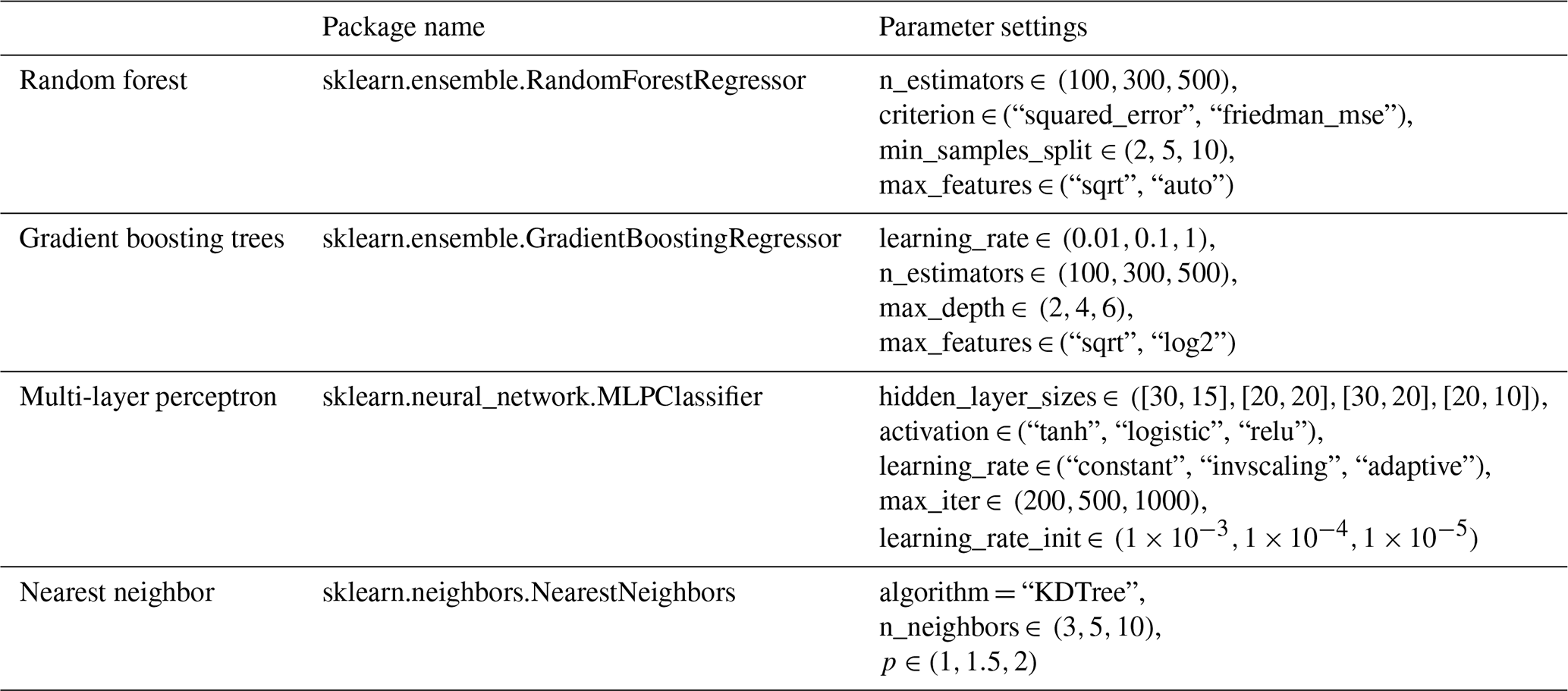
Having constructed the datasets (i.e., the optical flow AMVs and the simulated lidar information), we consider the topic of variable importance. There is a large body of literature on the topic, particularly for regression-based methods. Examples include approaches such as genetic algorithms, jackknifing, and forward selection (Bies et al., 2006; Lee et al., 2012; Blanchet et al., 2008). Here, due to the complexity of the functional model, we select our variable set using three different machine learning approaches that have been shown to be capable of modeling highly multivariate functional relationships: random forest (Breiman, 2001), gradient boosting regression trees (Friedman, 2001), and multi-layer perceptron (Gardner and Dorling, 1998). (Further details of parameter optimizations for these methods are discussed in Sect. 3.2 and Table 3.)

Table 3 Python package names (middle column) and the parameter settings for each of the method. Parameters not mentioned on this table are set as default in the Python methods. Note that the arrays under “Parameter settings” specify the option grid through which GridSearchCV is searching for the optimal choice.

Random forest and gradient boosting, in this case, employ decision trees (Kingsford and Salzberg, 2008), which is a popular and widely used machine learning algorithm that can be applied to both classification and regression tasks. Decision trees make predictions by mapping input features to output targets based on a series of binary decisions, and they form the basis of the two techniques considered in this section: random forest and gradient boosting trees. (For a more comprehensive overview of these machine learning methods, Chase et al., 2022, provides an excellent tutorial geared towards meteorologists.) The metric for variable importance for these two methods is constructed by keeping track of the decrease in accuracy or increase in impurity (e.g., Gini impurity for classification and increase in node purity for regression) caused by a chosen specific feature (Breiman, 2001). These purity-based variable importance plots, where higher values indicate greater importance, are shown in the first and second columns of Fig. 2 for random forest and gradient boosting trees, respectively. The variables' names on the x axis are described in Table 2.

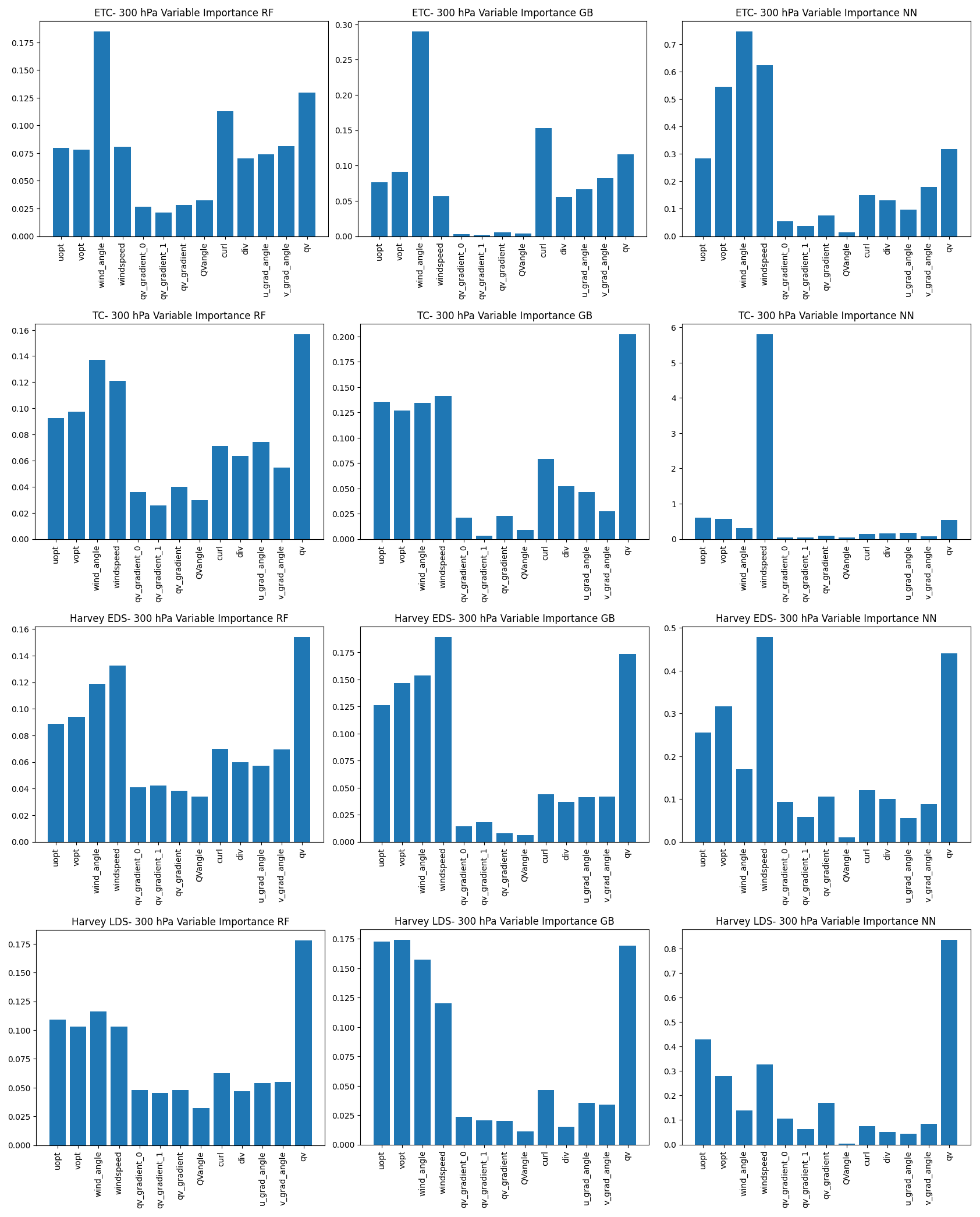
Figure 2 Variable importance plots for the 500 hPa pressure level at ETC, MCS, Harvey EDS, and Harvey LDS using three different approaches: random forest (left column), gradient boosting (middle column), and permutation with a neural network (right column). Higher values indicate higher importance. Variable names along the x axis are defined in Table 2.

The results from the left and middle columns of Fig. 2 indicate that the top five variables for regression are the retrieved optical flow winds, ($\widehat{u}$, $\widehat{v}$); wind speed and angle; and water vapor (q). We note that wind speed and wind angle are the polar-coordinate transform of the rectangular coordinates, ($\widehat{u}$, $\widehat{v}$), but their inclusion in the model significantly improves the model, since they provide an informative transformation that makes it easier for the machine learning model to model the functional form of interest.

One of the weaknesses of the purity-based variable importance plot is that high correlation between features can inflate the importance of numerical features (Gregorutti et al., 2017; Nicodemus et al., 2010) and that the purity-based variable importance is based only on training data and can have low or no correlation with independent validation data. To address these shortcomings, we supplement them with another approach based on permutation, which could be applied to any fitted estimator in tabular data contexts. The concept behind permutation feature importance involves quantifying the reduction in a model's score resulting from the random shuffling of a chosen variable (e.g., wind speed) while keeping all other variables the same within a fitted model (Breiman, 2001). The key insight is that if a model has significantly worse performance with a particular variable “shuffled”, then that variable must be important and the degree of importance can be assessed by the magnitude of the performance degradation. One advantage of this technique is that it could be applied to non-linear or opaque estimators, and for this we choose to apply it in conjunction with a neural network – specifically, a multi-layer perceptron regressor.

These permutation-based variable importance values are plotted in the right column of Fig. 2. The variable importance that comes out of the permutation method has a different unit and scaling compared to the purity-based variable importance, but both are consistent in indicating that higher values signify greater importance. The overall patterns are the same between different approaches, indicating that for the most part, the most important variables are $(\widehat{u}$, $\widehat{v})$, wind angle, wind speed, and water vapor content (q). Wind speed, however, is considered one of the most important predictors of bias according to the permutation method; one additional feature that is considered somewhat important in this metric is the curl. Therefore, we consider the set of these six variables in the following analysis and modeling.

3.2 Algorithm comparisons

Having identified the important predictive variables, we consider the algorithms for fitting the bias functional form. The features we require of the algorithm are able to handle complex multivariate data patterns, robust against new datasets and computationally fast. For this reason, we have chosen four methods that are known to do well for high-dimensional problems with complex relationships: random forest, gradient boosting trees, multi-level perceptron, and nearest neighbor. Here, we touch briefly on an overview of the methods before going into details of optimization and comparison. For readers who are not familiar with these machine learning approaches, we recommend the excellent tutorial series “A Machine Learning Tutorial for Operational Meteorology” (Chase et al., 2022, 2023).

Random forest is a powerful ensemble learning technique used for both classification and regression tasks in machine learning. As the name suggests, it consists of an ensemble of multiple decision trees, combining these trees to create a more accurate and robust predictive model (Breiman, 2001). Random forests are particularly popular due to their ability to handle complex data, reduce overfitting, and provide valuable insights into feature importance. Each tree is constructed using a random subset of the training data and a random subset of the input features. The predicted value, whether a class label or a regression value, is computed by passing the predictors to all the trees fitted within the model and aggregating the corresponding outcomes.

Gradient boosting trees is another powerful machine learning technique falling under the ensemble method umbrella. Like random forests, gradient boosting constructs an ensemble of decision trees, with each referred to as a “weak learner” because they are relatively simple and typically underfit on their own. However, the trees are built sequentially, with each new tree aiming to correct the errors made by the previous ones. Similar to random forests, gradient boosting aims to build many trees and is widely used for both regression and classification tasks because of its capacity to create accurate predictive models capable of handling complex data patterns (Friedman, 2001).

The multi-layer perceptron (MLP) is a foundational artificial neural network architecture that serves as the cornerstone for deep learning models. It is a versatile and powerful technique used for a wide range of machine learning tasks, including classification and regression. An MLP consists of interconnected layers of artificial neurons or nodes roughly divided into three types: input layers, which typically represent the predictors; hidden layers, responsible for processing information from the previous layer and extracting relevant features; and the output layer, which produces the final result, such as a classification label or a regression value. Each neuron processes information and passes its output to the next layer; the numeric parameters within each node, namely the weight and bias values, are estimated from the data using backpropagation and gradient descent (Gardner and Dorling, 1998).

Nearest neighbor methods operate on the principle of identifying a fixed number of training samples that are the closest in proximity to the new data point, and then predicting the label based on these identified neighbors. This number of samples can either be a user-defined constant, characteristic of k-nearest neighbor learning, or can adapt based on the density of nearby points, as seen in radius-based neighbor learning. The measurement of distance can be achieved through various metric measures, with the standard Euclidean distance being the most commonly selected option.

We used implementations of these methods from the Python scikit-learn package (version 1.2) (Kramer and Kramer, 2016). All of these methods require tuning of algorithm parameters, such as tree leaf nodes and depth for random forest and gradient boosting, hidden layer sizes, and activation methods for the neural network, neighbor size, and distance metrics for nearest neighbors, etc. To optimize these parameters, we employed the grid search optimization method from the scikit-learn package (sklearn.model_selection.GridSearchCV). This method iterates through different parameter choices provided in the parameter grid and identifies the best combination of parameters that minimize the loss function, which in this case is the root mean square error when fitted against the training data. The parameter search space for these four methods is detailed in Table 3.

To evaluate the performance of the four different methods, we divided the tabular datasets created from the data arrays into training datasets (used for model building) and validation datasets (used for performance assessment). We employed two types of division – spatial and temporal – as illustrated in Fig. 3. In the temporal division, we reserved the last $\mathrm{1}/\mathrm{4}$, $\mathrm{1}/\mathrm{3}$, and $\mathrm{1}/\mathrm{2}$ of the data using time stamps, respectively, and utilized these withheld data to evaluate performance in terms of RMSE. For the ETC dataset, spanning 12 h, this entailed setting aside the last 3, 4, and 6 h of data for validation.

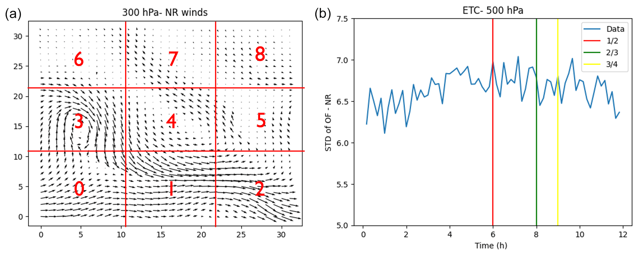
Figure 3 (a) Spatial validation scheme where the domain is divided into a 3 × 3 grid and labeled from 0 to 8. (b) Temporal validation scheme where the training data are set as the first $\mathrm{1}/\mathrm{2}$, $\mathrm{2}/\mathrm{3}$, and $\mathrm{3}/\mathrm{4}$ of the full dataset, respectively.

The results of this temporal validation for the ETC case are displayed in the right panels of Fig. 4. In all pressure levels, the machine learning approach consistently exhibits smaller bias than the uncorrected optical flow data, where bias is defined as the expected value of the difference between u wind from optical flow (both corrected and uncorrected) and the WRF-simulated truth. Notably, for the 300 and 500 hPa levels, the bias magnitude is significant at 2.5–3 m s⁻¹, but it is reduced to less than 0.5 m s⁻¹, signifying a substantial improvement. Similarly, although the reduction in bias is smaller at 850 hPa due to the optical bias starting at a lower value, the same trend persists.

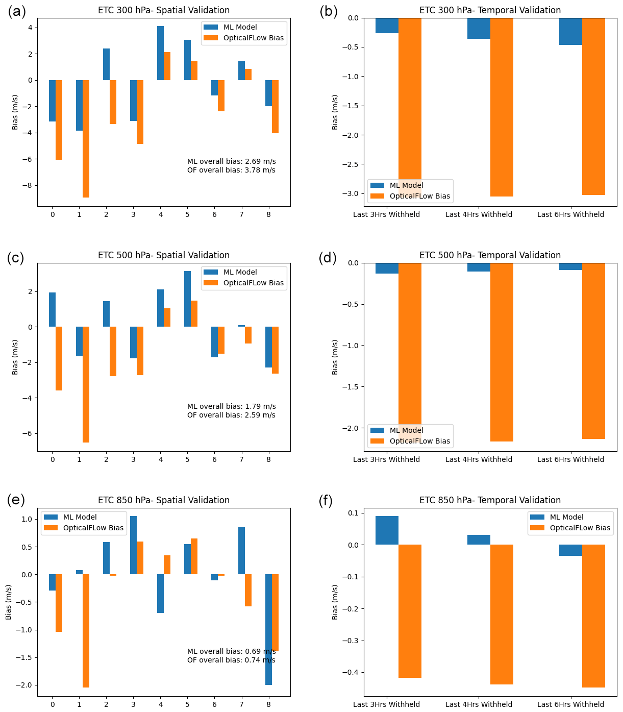
Figure 4 Sample plot of the random forest performance for ETC at three pressure levels for the (a, c, e) spatial case and (b, d, f) temporal case.

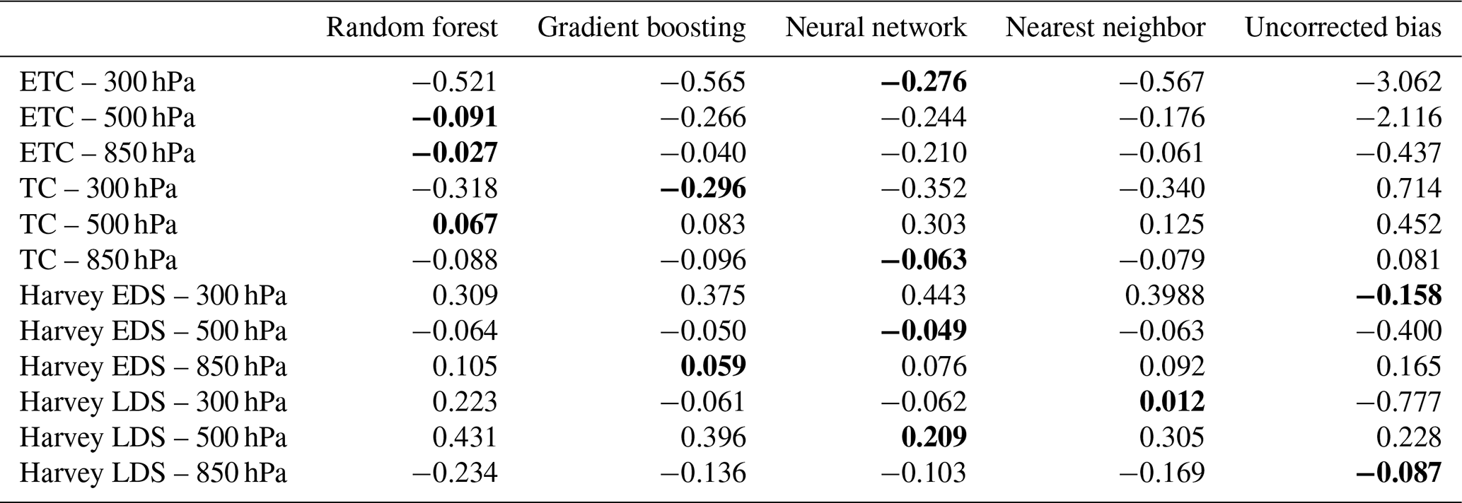
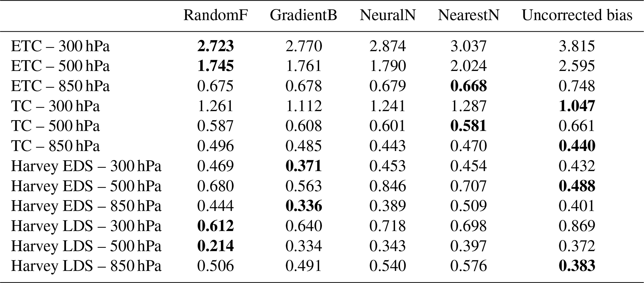
It is informative to assess the performance of all four algorithms across the four scenarios and three pressure levels. Therefore, we selected the case where $\mathrm{1}/\mathrm{2}$ of the data was withheld (considered the most challenging case) and summarized the validation performance in terms of bias for all four methods in Table 4. The scenarios at different pressure levels are listed in the rows. Overall, random forest, gradient boosting, and MLP tend to exhibit comparable performance, with no clear preference among the three. Nearest neighbor, on the other hand, consistently reduces bias relative to the uncorrected optical flow but falls short of the performance achieved by the other three algorithms. This suggests that the proximity-based methodology may not be flexible enough to capture the complex dependence structure of the AMV biases. We note that there are two instances where the uncorrected optical flow has the smallest bias (Harvey EDS 300 hPa and Harvey LDS 850), but these cases share a common feature in which the original optical flow exhibits a very low bias (< 0.25 m s⁻¹). In such cases, the algorithms may struggle due to the limited discernable signal for modeling.

Table 4 Validation temporal bias (computed from withheld last half of data for each atmospheric regime) for random forest, gradient boosting, neural network, and nearest neighbor. Units are in m s⁻¹. Cells that are in bold indicate the best performing method, which is defined as having bias that is closest to zero. The uncorrected bias is defined as the bias of the raw optical flow data relative to the WRF data.

Another validation approach is a purely spatial one. In this approach, we divide the domain of each study region (as seen in Fig. 1) into equal 3 × 3 areas and label each subregion with an index ranging from 0 to 8. In this labeling scheme, 0 represents the bottom-left cell, 2 the bottom-right cell, 4 the center cell, and 8 the top-right cell. We then withhold one of these nine regions at a time and train our models (e.g., random forest and gradient boosting) on the other eight cells. Subsequently, we apply our trained model to the withheld region. A sample of the results from these spatial validation efforts is shown in the left panels of Fig. 4 for the ETC case, using the random forest algorithm. In this figure, the indices on the axes represent the region that was withheld from the training process. The overall biases, computed in the lower-right of the panels, are mean absolute biases (MABs), which are defined as

$$\text{MAB}\left(m\right)=\sum _{i=\mathrm{1}}^{\mathrm{9}}{\displaystyle \frac{\left|b_i\right(m\left)\right|}{\mathrm{9}}},\text{where}{b}_i\left(m\right)=\sum _{j=\mathrm{1}}^{N_i}{\displaystyle \frac{\left({\widehat{u}}_{ij}^m-u_{ij}\right)}{N_i}}.$$

In this formula, m represents the methodology being evaluated (e.g., random forest, gradient boosting, and optical flow), b_i(m) denotes the normal bias when applying methodology m to the ith withheld dataset, and N_i stands for the number of observations within the ith validation dataset. The reason for calculating the mean absolute biases across these nine regions is to account for the possibility of biases having both positive and negative values. Therefore, we take the absolute value before averaging to prevent negative biases from canceling out positive biases and potentially distorting the resulting metrics.

The results from the ETC case in Fig. 4 indicate that, for most of the regions, the trained model results in biases that are smaller in magnitude than those of the original optical flow u wind. In some cases, the improvement in bias can be substantial (e.g., region 1). While, in a few instances, the RF model can result in biases with increased magnitude, this adverse effect is generally small compared to the magnitude of gains observed in other regions. The MABs are displayed in the lower-right corner of the left panels in Fig. 4, and they suggest that random forest consistently reduces the magnitude of the bias compared to the optical flow data. Another observation is that the validation spatial biases in Table 5 tend to be bigger than the validation temporal biases in Table 4 (e.g., the typical MAB in the spatial case is around 1.5 m s⁻¹, while the typical bias in the temporal validation case is around 0.5 m s⁻¹). In both cases, the machine-learning-corrected values tend to be improved over the uncorrected optical flow data, indicating that the algorithm is able to capitalize on information within the training dataset for both the spatial and temporal case. However, their difference in performance in Tables 4 and 5 indicates that functional relationship between the biases and the predictive variables in Sect. 3.1 may change depending on the spatial region, which makes sense intuitively since different regions of a storm system might exhibit different bias characteristics. However, this functional relationship, as demonstrated by Table 4, tends to be much more stable in terms of temporal evolution in the timescales that we examined (i.e., 3, 4, and 6 h in advance), which allows the algorithms considered to be more accurate in predicting and correcting the biases.

Table 5 Validation spatial bias (averaged over all nine spatial regions) for random forest, gradient boosting, neural network, and nearest neighbor. Bias is computed as the mean of absolute bias within each of the spatial region. Cells that are bolded indicate the best-performing method, which is defined as having bias that is closest to zero.

In Table 5, we present the MABs of the four algorithms (as well as that of the uncorrected optical flow) across the four scenarios and pressure levels. We observe the same overall patterns as in the temporal validation shown in Table 4, noting that random forest, gradient boosting, and MLP tend to exhibit the best performance, although their dominance varies across different scenarios and pressure levels. As before, nearest neighbor does not produce notably superior results. In some cases, the uncorrected optical flow algorithm has the lowest error, but these tend to be cases where the bias initially starts off at a low level.

3.3 Uncertainty characterization of AMVs

In data assimilation, thinning high-density AMVs is often necessary. Typically, this process involves giving preference to vectors that exhibit higher accuracy. The selection procedure usually takes into consideration various indicators of error level associated with the vectors, such as the quality indicator (QI), expected error (EE), recursive filter flag (RFF), and error flag (ERR) (Le Marshall et al., 2004). All of these metrics share the common goal of grouping AMVs with similar errors together, meaning that observations with good quality indicators should all exhibit low errors relative to the unobserved truth.

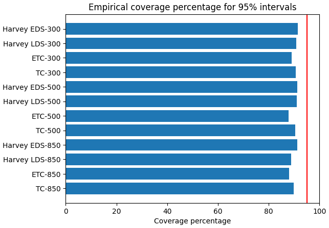
Figure 5 Actual coverage percentage of the 95 % prediction intervals when evaluated against withheld validation data. The vertical red line is the ideal coverage percentage as implied by the 95 % intervals.

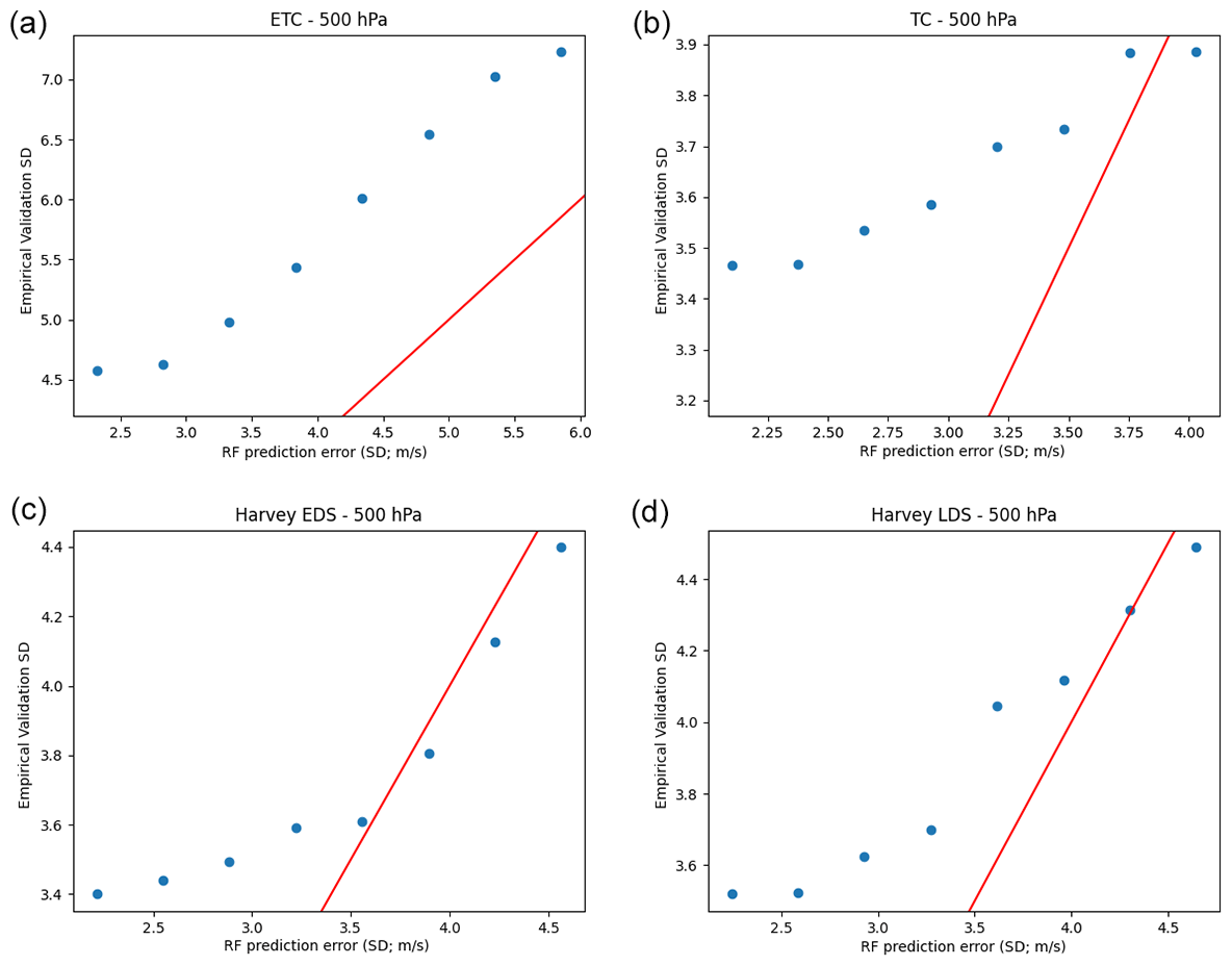
Figure 6 Plots of the estimated prediction error from random forest versus empirical validation error using quantile random forest for (a) ETC, (b) TC, (c) Harvey EDS, and (d) Harvey LDS. Red lines are the identity (y=x) lines.

We note that pattern tracking and optical flow do not provide an intrinsic error estimate, necessitating the addition of the post hoc error indicators mentioned above. In the existing remote sensing literature, a variant of random forest called quantile random forest has been extensively used to model uncertainty alongside the prediction of interest (e.g., a digital soil mapping product – Vaysse and Lagacherie, 2017; soil organic matter – Nikou and Tziachris, 2022; nitrogen use efficiency – Liu et al., 2023). In this section, we shall employ quantile forest regression to construct the prediction intervals for the u wind and compare them with withheld validation u-wind data.

Quantile random forest, as introduced by Meinshausen and Ridgeway (2006), is a modification of the random forest procedure that enables the estimation of prediction intervals for the intended variables. In contrast to normal random forests, which approximate the conditional mean of a response variable, quantile random forests (QRFs) provide the full conditional distribution of the response variable to construct prediction intervals. (For readers who are not familiar with the random forest algorithm, Chase et al. (2022) provides an excellent meteorology-geared tutorial.) The key insight that allows for this property is that while random forests solely retain the mean of observations within each node and discard any additional information, quantile random forests preserve the values of all observations within the node (not just their mean) and use these distributions to make estimates of the quantiles of interest. In particular, Meinshausen and Ridgeway (2006) prove that the conditional quantile estimates are asymptotically consistent under specific assumptions:

• 1.

  The proportion of values in a leaf, relative to all values, vanishes as the number of observations, n, approaches infinity.

• 2.

  The minimal number of values in a tree node grows as n approaches infinity.

• 3.

  When looking for features at a split, the probability of a feature being chosen is uniformly bounded from below.

• 4.

  There is a constant, γ, in the range $\mathit{\gamma }\in (\mathrm{0},\mathrm{0.5})$ such that the number of values in a child node is always at least γ times the number of values in the parent node.

• 5.

  The conditional distribution function is Lipschitz continuous with positive density.

These are fairly modest assumptions, particularly with respect to the construction of the trees. However, it is worth noting that the quantiles under these assumptions are only asymptotic consistent as n approaches infinity. However, these assumptions provide some theoretical assurance that the outputs of quantile random forest should approximate the true conditional quantiles to some extent.

Here we use the Python implementation of QRF provided by the Python package quantile-forest. We use quantile random forest to build 95 % prediction intervals at the pixel level. That is, at any pixel, we compute the prediction interval as follows:

$$I\left(\mathit{x}\right)=\left[Q_{.025}\left(\mathit{x}\right),Q_{.975}\left(\mathit{x}\right)\right],$$

where Q_.025(⋅) and Q_.975(⋅) are the 2.5th percentile and 97.5th percentile random forest estimators from quantile-forest, respectively, and x is the vector of predictors (e.g., optical flow winds, wind speed, and angle), as discussed in Sect. 3.1.

We wish to assess the performance of the intervals, I(x), given by quantile random forest, and one approach is to compute the coverage probability of the confidence intervals when applied to withheld simulated lidar data. We repeat the exercises in the previous section, and for each of the four scenarios and three pressure levels, we use the first half of the storm for training and the second half for validation. We then compute the coverage percentage of the prediction intervals, which is defined as the probability (expressed as percentage) that the true u wind actually falls within the interval given by quantile random forest. That is, the coverage percentage (CP) for a given scenario and pressure level is given by

$$\text{CP}={\displaystyle \frac{{\sum }_{i=\mathrm{1}}^N\textcolor{red}{}\left(Q_{.025}\left({\mathit{x}}_i\right)\le u_i\cap u_i\le Q_{.975}\left({\mathit{x}}_i\right)\right)\cdot \mathrm{100}}{N}},$$

where u_i is the ith WRF wind from the withheld validation set, $\textcolor{red}{}(\cdot )$ is the indicator function, and N is the size of the validation dataset. A comparison of the coverage probability for all scenarios and pressure levels is given in Fig. 5. There, we see that the 95 % prediction intervals from quantile random forest consistently underestimate the magnitude of the error variability, averaging between 85 % and 90 % coverage, while the ideal number should be 95 %. This implies that the prediction interval widths given by quantile random forest in general tend to be a bit smaller than what the validation data require.

To get a clearer idea of the differences between the estimated prediction error and that of the validation data, we examine their relationship in a scatter plot. To do so, we first convert the prediction intervals, I(x), to their effective prediction error, $\widehat{\mathit{\sigma }}\left(\mathit{x}\right)$. This conversion relies on the fact that in a Gaussian distribution, the 95 % confidence interval is given by a ±2 standard deviation of the mean. Therefore, to compute the effective prediction error from our 95 % confidence interval, we divide the interval width by 4. That is,

$$\widehat{\mathit{\sigma }}\left(\mathit{x}\right)={\displaystyle \frac{Q_{.975}\left(\mathit{x}\right)-Q_{.025}\left(\mathit{x}\right)}{\mathrm{4}}}.$$

To compare this effective prediction error, $\widehat{\mathit{\sigma }}\left(\mathit{x}\right)$, against the withheld validation data, we construct the equivalent standard error using the withheld validation data. We use the binning approach, where the empirical validation error (EVE) for a given prediction error value, σ, and a given bin length, d, is computed by aggregating all observations where the QRF prediction error is within ±d of σ, and then we compute the RMSE on this subset. In formal terms, the EVE is given by

$$\begin{array}{}\text{(2)}& \text{EVE}(\mathit{\sigma },d)=\sqrt{\left(\sum _{i\in \left|\widehat{\mathit{\sigma }}\right({\mathit{x}}_i)-\mathit{\sigma }|<d}{\displaystyle \frac{{\left(u_i^{*}-u_i\right)}^{\mathrm{2}}}{N}}\right)},\end{array}$$

where $u_i^{*}$ is the ith RF-corrected u wind in the validation dataset, u_i is the ith true WRF u wind, and N is the size of the validation dataset.

With the formulas above, we binned the RF prediction errors into eight equally spaced bins and computed the corresponding EVE. The results are shown for all scenarios at the 500 hPa pressure level in Fig. 6. Although the overall patterns are similar at other pressure levels, this figure provides a more nuanced view, showing that while the RF prediction errors tend to under estimate the true errors, they exhibit a statistically significant linearly increasing relationship. This is a valuable property. It implies that while the errors are not accurate (i.e., statistically valid), their positive correlation with the true error indicates that we can use the QRF prediction error as a proxy for quality assessment.

To demonstrate the usefulness of this property, we simulate a quality indicator flag by dividing the validation data into three equal-size categories: low-, mid-, and high-quality. The three categories are constructed by sorting the QRF prediction errors (or alternatively the prediction interval widths) from smallest to largest and then classifying the smallest one-third as high-quality, the middle one-third as mid-quality, and the largest one-third as low-quality. We then compute the EVE of the optical flow wind versus the withheld true wind within each bin, and we display the results in Table 6. Intuitive understanding of high-quality observations generally implies that they are more accurate than low-quality observations; indeed, here, Table 6 indicates that the EVE values, for every region and every pressure level, form an increasing pattern with high-quality observations having the smallest error, mid-quality having medium error, and low-quality having the largest error.

Table 6 SD vs. quality indicators based on RF prediction errors. Baseline SD is defined as the SD of the entire optical flow dataset against the WRF-simulated truth. (i.e., SD$(\widehat{u}-u)$).

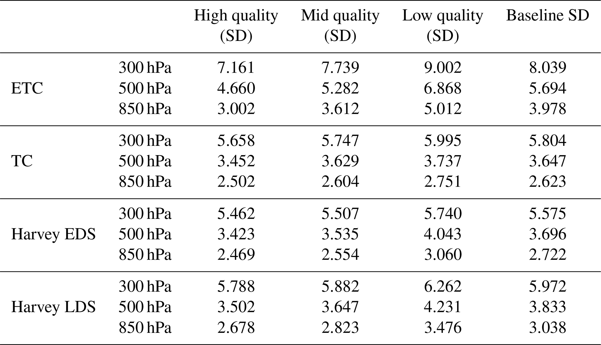
The differences between the high-quality and low-quality observations can be fairly small some situations, particularly for the TC case at all pressure levels. We note that this is because of the design of the experiment. Recall that we are using withheld simulated lidar data that have added Gaussian zero mean random errors with pressure-dependent standard deviations: 2 m s⁻¹ for 850 hPa, 3 m s⁻¹ for 500 hPa, and 5 m s⁻¹ for 300 hPa. These random measurement errors are added to all quality categories, which then essentially dilute the contribution of the variability coming from the bias signal. This explains why the differences between high-, medium-, and low-quality bins are larger when the measurement errors are relatively low.

We note that the experiment in Table 6 divided the data into three bins. In general, the results here should hold for different numbers of bins although a high single-digit number might be unstable. A hint of this instability is seen in Fig. 6, where we observe that for the top-right panel, the rightmost bin has almost an identical EVE compared to the bin immediately preceding it. This may be due to the fact that there are low bin counts at the extreme edge of the domain. In general, increasing the bin count can reduce the bin counts, exacerbating these statistical artifacts. However, quality indicators in common usage tend to use a low single-digit number of bins, which works well here.

4 Conclusions

Accurately estimating global wind patterns is of paramount importance across scientific and practical domains, including applications like global chemical transport modeling and numerical weather prediction. Atmospheric motion vectors (AMVs) serve as crucial inputs for these applications. However, addressing errors in AMV retrievals becomes imperative before their assimilation into data assimilation systems, as these errors can significantly impact output accuracy. One noteworthy error characteristic of AMVs is bias, which varies considerably by region. These biases can lead to adverse results if the AMVs are incorporated into data assimilation systems without proper mitigation or bias removal.

In real-world applications, correcting the bias in AMV retrievals necessitates an independent benchmark or reference to establish accuracy. Independent data sources may include collocated radiosonde data or lidar AMV data, such as those available from Aeolus. In this paper, we present a proof of concept that demonstrates the feasibility and performance of a bias-correction scheme within an observing system simulation experiment (OSSE) framework. Specifically, we examined three different storm systems in the Gulf of Mexico, North Atlantic Ocean, and southeast Asia and applied our bias correction and prediction error interval procedure to outputs generated by a novel AMV algorithm known as optical flow. Our results suggest that passive-sensor AMVs, which typically have high coverage but low precision, can benefit significantly from coincident high-precision active-sensor wind data. These benefits can be harnessed through algorithms that model expectations (bias reduction) or quantiles (uncertainty quantification).

In Sect. 3.2, we demonstrate that conventional machine learning algorithms such as random forest and gradient boosting can effectively learn the complex multivariate dependence structure of errors and correct biases in raw optical flow AMVs. It is worth noting that despite having low bias in some cases, the standard deviation of the AMV error can be relatively large (e.g., with a standard deviation of 1–2 m s⁻¹, while the error may be on the scale of < 0.5 m s⁻¹). In these scenarios, the error-correction model produces biases of a similar magnitude (i.e., < 0.5 m s⁻¹). Notably, we show that in the storm systems we considered, it is possible to estimate biases with minimal performance degradation up to 6 h in advance.

One of the most valuable extensions of machine learning models in this bias-correction exercise is the ability to estimate prediction intervals. In Sect. 3.3, we employ the quantile random forest framework by Meinshausen and Ridgeway (2006) to generate prediction intervals for withheld validation data. We observe that while the prediction intervals often tend to be too narrow (underestimating the variability in the true process), they generally exhibit a monotonically increasing relationship with the NatureRun wind variability. In other words, the uncertainty estimates from the quantile random forest are not statistically valid (i.e., the 95 % confidence intervals may not capture the truth 95 % of the time), but the algorithm does correctly rank the error magnitudes when analyzing multiple pixels. Therefore, while the prediction intervals may not be directly usable in data assimilation, they can serve as valuable components of a quality indicator. Indeed, in Sect. 3.3, we conduct an experiment where we categorize the optical flow retrievals into three groups – high-, mid-, and low-quality. We demonstrate that the standard deviation within these categories relative to the validation data follows an increasing pattern, with high-quality observations having the lowest error standard deviation, mid-quality observations falling in the middle range, and low-quality observations displaying the highest error standard deviation.

These results are highly promising, particularly regarding the application of quantile random forest in quality indicators. Our future research plans involve extending this study to other global regions and various convective systems. It is worth noting that different applications or study regions may necessitate distinct sets of predictive variables and that the selection of variables employed in our feature selection process may not be universally applicable. Nevertheless, the same variable selection process presented in Sect. 3.1 can be adapted to determine the most relevant predictive variables. In this paper, we utilized quantile random forest for prediction interval estimation, but theoretically, other machine learning algorithms could be employed to generate quantiles (e.g., quantile neural networks), although the computational requirements may vary.