the Creative Commons Attribution 4.0 License.
the Creative Commons Attribution 4.0 License.
 | 03 Jul 2024
Fast retrieval of XCO2 over east Asia based on Orbiting Carbon Observatory-2 (OCO-2) spectral measurements
Fengxin Xie
Tao Ren
Changying Zhao
Yilei Gu
Minqiang Zhou
Pucai Wang
Kei Shiomi
Isamu Morino
The increase in greenhouse gas concentrations, particularly CO2, has significant implications for global climate patterns and various aspects of human life. Spaceborne remote sensing satellites play a crucial role in high-resolution monitoring of atmospheric CO2. However, the next generation of greenhouse gas monitoring satellites is expected to face challenges, particularly in terms of computational efficiency in atmospheric CO2 retrieval and analysis. To address these challenges, this study focuses on improving the speed of retrieving the column-averaged dry-air mole fraction of carbon dioxide (XCO2) using spectral data from the Orbiting Carbon Observatory-2 (OCO-2) satellite while still maintaining retrieval accuracy. A novel approach based on neural network (NN) models is proposed to tackle the nonlinear inversion problems associated with XCO2 retrievals. The study employs a data-driven supervised learning method and explores two distinct training strategies. Firstly, training is conducted using experimental data obtained from the inversion of the operational optimization model, which is released as the OCO-2 satellite products. Secondly, training is performed using a simulated dataset generated by an accurate forward calculation model. The inversion performance and prediction performance of the machine learning model for XCO2 are compared, analyzed, and discussed for the observed region over east Asia. The results demonstrate that the model trained on simulated data accurately predicts XCO2 in the target area. Furthermore, when compared to OCO-2 satellite product data, the developed XCO2 retrieval model not only achieves rapid predictions (<1 ms) with good accuracy (1.8 ppm or approximately 0.45 %) but also effectively captures sudden increases in XCO2 plumes near industrial emission sources. The accuracy of the machine learning model retrieval results is validated against reliable data from Total Carbon Column Observing Network (TCCON) sites, demonstrating its ability to effectively capture CO2 seasonal variations and annual growth trends.
- Article
(8164 KB) - Full-text XML
- BibTeX
- EndNote


Since the Industrial Revolution, human activities have released large amounts of greenhouse gases, primarily carbon dioxide, into the atmosphere. This continual increase in emissions has led to global warming and has disrupted human societies and ecosystems (Zehr, 2015). Accurately estimating atmospheric carbon fluxes is critical for implementing effective emission reduction strategies at national and regional levels. However, precise carbon flux estimates require assimilating carbon dioxide concentration data across regions using measurements of atmospheric column-averaged dry air-mole fraction of carbon dioxide (XCO2; Jin et al., 2021). Direct measurement methods like balloons or aircraft have challenges obtaining global-scale data. Currently, the main monitoring approach uses spectrometers to record spectra in CO2 absorption bands, followed by inversion algorithms to derive XCO2. The two primary monitoring methods are ground-based monitoring stations and satellite remote sensing.
The Total Carbon Column Observing Network (TCCON) provides ground-based monitoring of atmospheric carbon dioxide through a global network of high-precision Fourier transform spectrometers (Wunch et al., 2011, 2015). However, TCCON sites are sparsely distributed and cannot be deployed in regions with unfavorable geography or harsh climates. Consequently, the network lacks the extensive spatial coverage required for comprehensive global carbon monitoring and carbon cycle analysis. Nevertheless, the ultra-high spectral resolution of TCCON spectrometers enables highly accurate retrievals of XCO2. Under clear-sky conditions, TCCON precision can reach 0.1 % (<0.4 ppm). Under relatively clear conditions with minimal clouds and aerosols, precision remains within 0.25 % (<1 ppm; Messerschmidt et al., 2011). Due to such high precision and accuracy, TCCON data are invaluable for validating satellite-based XCO2 products (Cogan et al., 2012; Wunch et al., 2017; Liang et al., 2017) and comparing them to carbon cycle models. However, the spatial limitations of the network underscore the need for satellite remote sensing to provide regular global measurements of atmospheric carbon dioxide.
High-spectral-resolution greenhouse gas monitoring satellites employ spectrometers in orbit to measure solar radiation spectra after interaction with the Earth's atmosphere and ground surface (Meng et al., 2022). Unlike ground monitoring, satellite remote sensing offers broader spatial coverage and more flexible temporal observation globally. Consequently, satellite remote sensing has become vital for greenhouse gas monitoring worldwide. Notable ongoing passive CO2 observation missions include China's TanSat (Liu et al., 2018), Japan's Greenhouse Gases Observing Satellite (GOSAT, 2009) and GOSAT-2 (2018) (Hamazaki et al., 2005; Kuze et al., 2009; Imasu et al., 2023), and the United States' OCO-2 (2014) and OCO-3 (2018; Crisp et al., 2017; Eldering et al., 2019). Upcoming missions are France's MicroCarb by CNES (Cansot et al., 2023), ESA's CO2M (Sierk et al., 2021), and GOSAT-GW (Matsunaga and Tanimoto, 2022). The next-generation greenhouse gas monitoring satellites mainly address the challenge of improving the spatial and temporal resolutions of observations. However, single satellites still have resolution, coverage, and meteorological limitations for regional emission monitoring. Enhancing satellite sensor performance alone cannot produce datasets sufficient for monitoring carbon sources and sinks. Improving the accuracy and efficiency of satellite data inversion is also crucial. Integrating data from multiple satellites into a coordinated system is necessary to fully capture dynamic changes in regional carbon sources and sinks. Developing new high-precision, high-throughput inversion methods to efficiently derive accurate greenhouse gas concentration distributions from satellite data is a key challenge needing attention.
The mainstream inversion algorithms (O'Dell et al., 2012; Crisp et al., 2012; Yoshida et al., 2013) for retrieving greenhouse gas concentrations from high-spectral-resolution satellite measurements are based on nonlinear Bayesian optimization theory (Rodgers, 2000) and full physics models. In essence, these algorithms operate by iteratively adjusting estimated gas concentration profiles and other atmospheric and surface parameters in a radiative forward model to minimize the mismatch between simulated and observed spectra. More specifically, the inversion process starts with the a priori atmospheric state, including trace gas concentration profiles as functions of pressure/altitude. Radiative-transfer equations are then solved to simulate the top-of-atmosphere radiance spectrum observed by the satellite for this atmospheric state. The simulated spectrum is compared to the actual observed spectrum, calculating the difference, covariance, and cost function. The input gas profiles and model parameters are iteratively adjusted to reduce the cost function over multiple rounds of radiative-transfer simulations. Once simulated spectra closely match observations, the model state is output as the retrieved concentration profile. However, executing these complex optimizations requires computationally expensive interpolation of high-spectral-resolution gas absorption reference data and solving the radiative-transfer equations in each iteration. Running the radiative forward model repeatedly for every adjusted atmospheric state also leads to slow overall inversion. Consequently, optimization-based retrievals struggle to match increasing satellite observation volumes and throughput needs. This inherent inefficiency has become a major obstacle to operational greenhouse gas monitoring using current and planned high-resolution spectrometers. While rigorous, standard nonlinear optimization retrievals lack the speed and scalability required for high-precision real-time or near-real-time satellite-based greenhouse gas mapping. Overcoming this bottleneck necessitates new inversion approaches that can ingest high-resolution spectral data and retrieve concentrations with both accuracy and computational efficiency.
In recent years, machine learning has demonstrated exceptional performance across various research fields, with the discovery of potential nonlinear relationships between data as one of its fundamental and crucial applications. Regarding the important applications of carbon dioxide (CO2) retrieval, Carvalho et al. (2010) attempted to retrieve the vertical CO2 profiles using spectral data from SCIAMACHY's 6 channels (1000–1700 nm). The overall precision and bias of the retrieved results were estimated to be approximately 1.0 % and less than 3.0 %, respectively. Gribanov et al. (2010) developed a two-hidden-layer multilayer perceptron (MLP) model to retrieve CO2 vertical concentrations by reflected solar radiation measured by the GOSAT Thermal and Near infrared Sensor for carbon Observation – Fourier Transform Spectrometer (TANSO-FTS) sensor, achieving an inversion accuracy better than 1 ppm for CO2 column-averaged values and better than 4 ppm for surface CO2 concentrations for the test samples. In the study conducted by Zhao et al. (2022), a two-step machine learning approach was developed for retrieving atmospheric XCO2 using spectral data from the GOSAT weak-CO2 band. They established a direct one-dimensional line-by-line forward model to simulate GOSAT's observed spectra within the 6180–6280 cm−1 spectral interval, forming the foundation for training their machine learning model. The retrieval model operates by initially obtaining the atmospheric spectral optical thickness, followed by extracting XCO2 from these optical thickness spectra. As a proof-of-concept, the method was tested in Australia under clear-sky conditions using GOSAT's spectra, demonstrating an accuracy of approximately 3 ppm for XCO2 retrieval. The study also discussed potential enhancements to further refine the accuracy of this retrieval method. Keely et al. (2023) employed the machine learning method of Extreme Gradient Boosting (Chen and Guestrin, 2016) to develop a nonlinear bias correction approach for the OCO-2 version 10 product, significantly reducing systematic errors in CO2 measurements and improving data quality, with an increase in sounding throughput by 14 %. David et al. (2021) and Bréon et al. (2022) attempted to establish correlations between XCO2 in the European Centre for Medium-Range Weather Forecasts CAMS (Copernicus Atmosphere Monitoring Service) database and OCO-2 satellite monitoring spectra using multilayer perceptron artificial neural network models. However, their recent research (Bacour et al., 2023) indicates that when the test dataset extends beyond the time range covered by the training dataset, the predicted results show a slight bias, approximately 2.5 ppm yr−1. Practical deployment of machine learning techniques for remote sensing demands additional research into the generalization performance of models on new observational data distributions beyond those encountered during training.
In the present paper, a proof-of-concept study demonstrates a novel machine learning strategy to accurately and efficiently retrieve atmospheric XCO2 values from OCO-2 satellite spectral measurements. The model rapidly retrieves XCO2 directly from OCO-2 spectral data, eliminating the need for repetitive radiative-transfer simulations required by traditional nonlinear optimization retrieval algorithms. Additionally, the model enables the prediction of future XCO2 values. The method was validated by comparing the retrieved XCO2 against OCO-2 satellite version 10r products and ground-based TCCON measurements, confirming the accuracy of our efficient spectral-inversion approach. The model also successfully demonstrated its ability to detect local plume features, indicating its potential utility in monitoring and analyzing specific emission sources. A major innovation in the present study is using accurate radiative-transfer simulations to generate the training data rather than relying solely on experimental data products. This simulation-based training approach could help overcome limitations in existing experimental data. Additionally, our neural network model achieves XCO2 retrieval speeds orders of magnitude faster than traditional methods, reducing computation time from multiple seconds to less than 1 ms. This dramatic improvement in retrieval efficiency could enable real-time processing of the massive data volumes expected from next-generation greenhouse gas monitoring satellites. Importantly, our model achieves a precision of less than 1.8 ppm, competitive with the current state of the art in retrieval accuracy. We also demonstrate the ability to accurately capture temporal variations and trends in XCO2 by validating against reliable TCCON ground-based data. This level of verifiable performance is an important ability. This provides an effective solution for rapid inversion of large-scale high-spectral-resolution remote sensing data in the future.
2.1 Targeted area and data screening
This proof-of-concept study aims to develop and validate an accurate and efficient machine-learning-based XCO2 retrieval model applied to the long OCO-2 time series for the east Asian region. Currently, similar global XCO2 retrieval models rely on computationally intensive physical models. Our goal is to demonstrate a more efficient data-driven approach using MLP neural networks.
Before developing the machine-learning-based fast-retrieval model, we implemented several preprocessing steps on the OCO-2 observational dataset (OCO-2 Science Team et al., 2020a) for the target east Asian area spanning between 20–45° N and 110–145° E, as shown in Fig. 1. Specifically, we filtered the data both spatially and temporally to focus only on observations within the geographic region and time period of interest (2016–2021). Additionally, we filtered the data to only include nadir mode observations marked as “good” based on the quality flag indicator (“xco2_quality_flag” = 0 in OCO-2 Lite v10r files; OCO-2 Science Team et al., 2020b), as these represent the highest quality OCO-2 measurements.
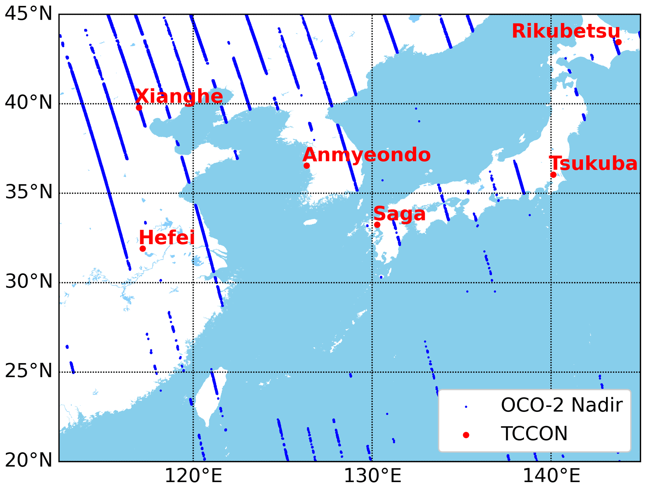
Figure 1The target area for the east Asia region, distribution of observation points (from OCO-2 L2 std v10r files) of OCO-2 nadir mode in January 2016, and the distribution of TCCON sites in this area.
Several TCCON ground stations located in this region (e.g., Hefei, Saga, Tsukuba, Xianghe, Anmyeondo, and Rikubetsu), as shown in Fig. 1, provide valuable ground-truth XCO2 data for validating the MLP model predictions. If the model can accurately reproduce the TCCON observations from corresponding OCO-2 measurements, it suggests that the model has learned meaningful relationships between the satellite data and underlying CO2 concentrations.
Furthermore, the successful demonstration of accurate XCO2 retrieval over east Asia is a first step toward expanding this approach globally. The model could be retrained or supplemented with additional regional data to extend coverage. By combining reliable regional MLP models, global XCO2 maps could be retrieved. This “jigsaw puzzle” strategy would further validate the feasibility of global-scale machine-learning-based XCO2 retrievals from satellite observations.
2.2 The artificial neural network architecture
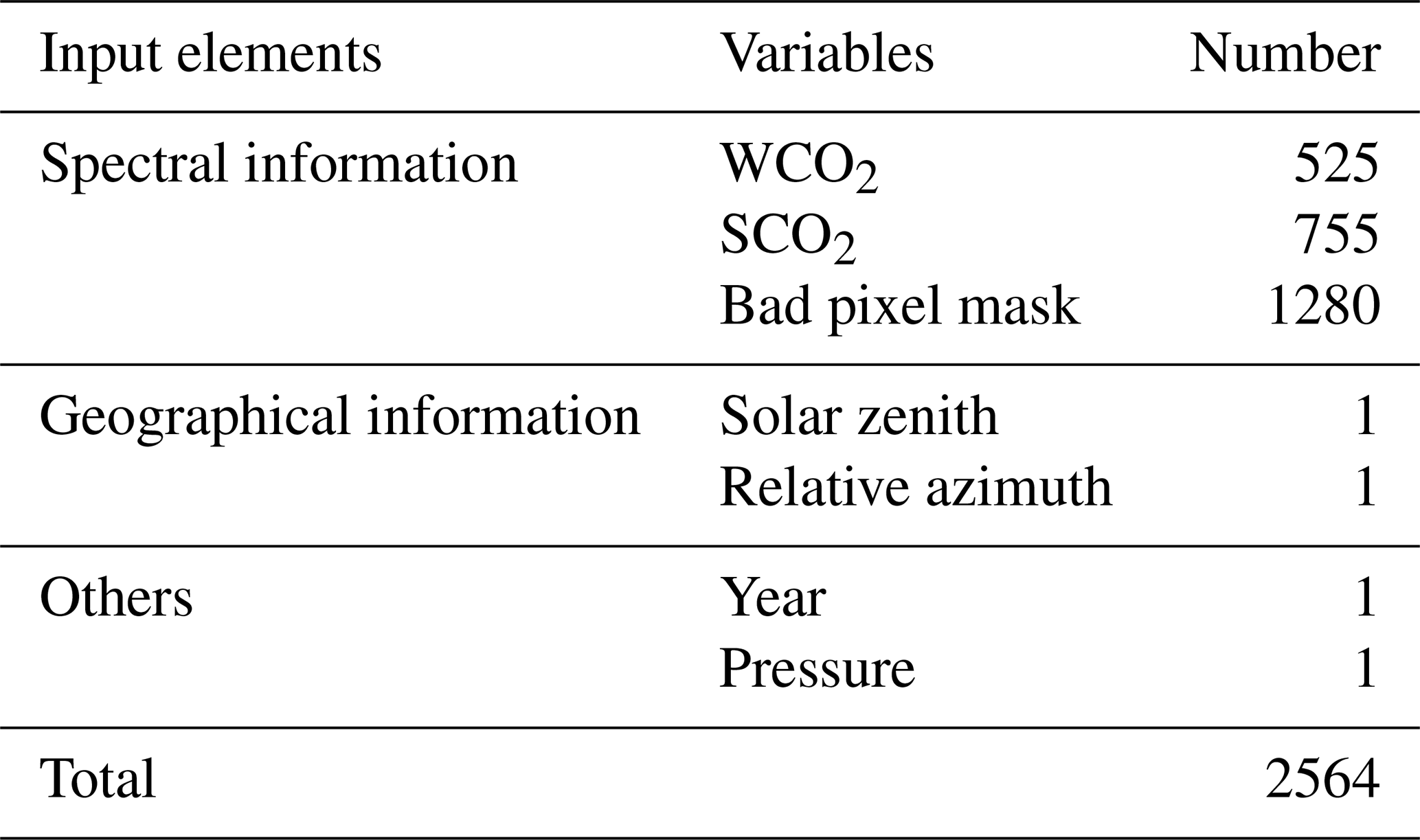
This study introduces a multilayer perceptron (MLP) neural network model for estimating XCO2 from OCO-2 satellite observations. Inspired by David et al. (2021) and Bréon et al. (2022), the MLP-XCO2 model input layer is designed based on the measurement principles of OCO-2 and atmospheric radiative-transfer effects on the observed spectra; the artificial neural networks architecture is shown in Fig. 2. Specifically, the MLP model input layer consists of spectral information, surface pressure, the corresponding year, and geographical observation information, as summarized in Table 1 and explained below.
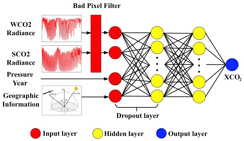
Figure 2Schematic diagram of the MLP-XCO2 model. The input layer includes two interpolated radiance values of WCO2 and SCO2 band filtered through a bad pixel filter, geographical observation information, surface pressure, and the corresponding year. A dropout layer with a 0.1 dropout rate is added between the input layer and the first hidden layer.
Table 1A detailed list of the input parameters for the MLP-XCO2 model.
2.2.1 Spectral information
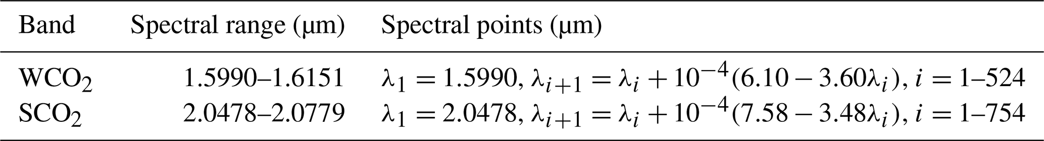
The OCO-2 satellite instrument measures high-resolution spectra in three spectral bands centered around 0.76, 1.6, and 2.0 µm, referred to as the O2-A, weak CO2 (WCO2), and strong CO2 (SCO2) bands, respectively (OCO-2 Science Team et al., 2019). However, only the WCO2 and SCO2 bands are used as inputs for current XCO2 retrievals. The O2-A band is excluded as it lacks significant information needed to directly estimate XCO2 based on radiative-transfer principles. Instead, the O2-A band is primarily used in OCO-2's operational full-physics algorithm for rapid cloud and aerosol screening prior to CO2 retrieval (O'Dell et al., 2012), effectively excluding observational cases that potentially lead to poor retrieval quality, thus saving substantial computational costs. Each OCO-2 spectral band is sampled by 1024 detector pixels. However, over time some detectors have degraded or become unstable in the space environment, resulting in pixels being flagged as “bad samples” in quality filters (Marchetti et al., 2019). To maximize high-quality training data, additional preprocessing is performed on the WCO2 and SCO2 bands. Initially, the beginning and ending spectral ranges corresponding to the most degraded detectors are removed. The remaining spectra are resampled into 525 and 755 wavelength points for the WCO2 and SCO2 bands, respectively (spectral points in wavelength are detailed in Table 2). To enhance the CO2 absorption line information, each input spectrum is normalized by dividing the mean radiance within a nearby spectrally transparent window lacking absorption features (1.6056–1.6059 µm using 10 points for WCO2; 2.0602–2.0607 µm using 15 points for SCO2). Additionally, as shown in Fig. 3, we noticed that some isolated pixels within the main CO2 absorption bands still consistently exhibited poor radiance quality. To address this issue, a “bad sample filter” was implemented, which utilizes a binary record from the OCO-2 L1B database (0 indicates spectra derived from good-quality pixels, and 1 indicates pixels with defects or derived from poor-quality interpolations). The settings of this filter are determined solely by the historic records and the version of the bad-pixel map, ensuring refined data quality and consistency across different versions of the map. To further address bad samples resulting from natural degradation, we have implemented a dropout layer between the initial and the first intermediate MLP layer, thus enhancing the model generalizability with the remaining spectral inputs.
2.2.2 Geographical information
The model is designed to accept two key observation geometry angles that are determined by the relative positions of the Sun, the satellite, and the ground observation point. These include the solar zenith angle and relative azimuth angle. The solar zenith angle (SZA) features prominently as a cosine term in the radiative-transfer equation that defines the atmospheric radiative processes. Thus, SZA is pre-converted to its cosine form for model input. The relative azimuth angle is a comprehensive angle that jointly combines the solar azimuth angle and the satellite azimuth angle. It is important to emphasize that the satellite zenith angle is not used in this study. Our current research is based on the nadir mode of the OCO-2 satellite observation. In the nadir observing mode, the satellite zenith angle is assumed to be nearly perpendicular to the Earth's surface, theoretically approaching 0°.
2.2.3 Other parameters
In addition to the primary inputs, two other parameters play critical roles in the MLP-XCO2 model: the surface pressure and the corresponding year (2016, 2017, etc.). In traditional retrieval algorithms based on iterative optimization, accurate surface pressure and a reliable prior CO2 profile are crucial. The importance of this has been highlighted by the averaging kernel utilized in the OCO-2 retrieval algorithm (Nguyen et al., 2014), which indicates a higher sensitivity near the surface compared to the stratosphere. To prevent the retrieval of unrealistic CO2 profiles, the prior covariance matrix imposes significantly stricter constraints in the stratosphere than in the troposphere (O'Dell et al., 2012). In cases where the prior CO2 profile is inadequate, it can lead to poor results, with minimal or even opposite updates in the stratospheric CO2 profile during the inversion process (Iwasaki et al., 2019). Additionally, in order to achieve the best agreement between observed and estimated spectra, the retrieval process may inaccurately estimate tropospheric CO2 profiles. To tackle these challenges, our investigation suggests that incorporating additional information such as the year can offer valuable context for XCO2 retrieval. This conservative approach provides a simple means to enhance prior CO2 information without directly specifying XCO2 prior values.
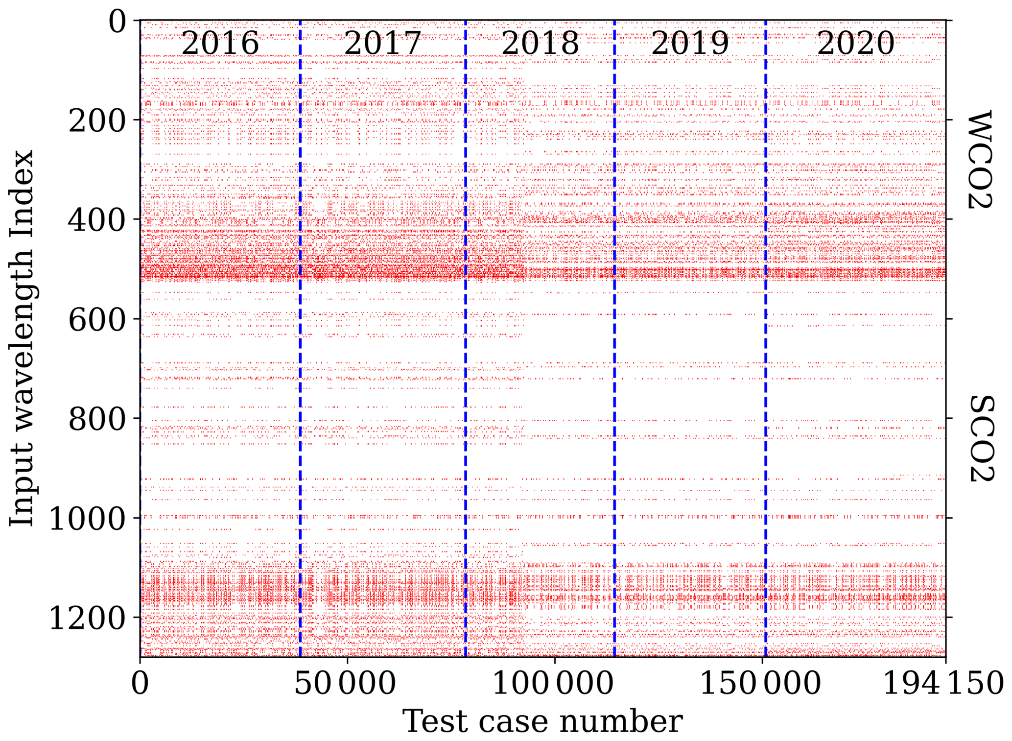
Figure 3Visualization of the OCO-2 satellite data quality across interpolated wavelength grid indices. The map illustrates the bad-sample list extracted from OCO-2 Level 1B files for all test cases. On the horizontal axis, sample numbers range from 0 to 194 150, while the vertical axis represents various wavelength grid indices ranging from 0 to 1280. Red coloration indicates problematic data pixels.
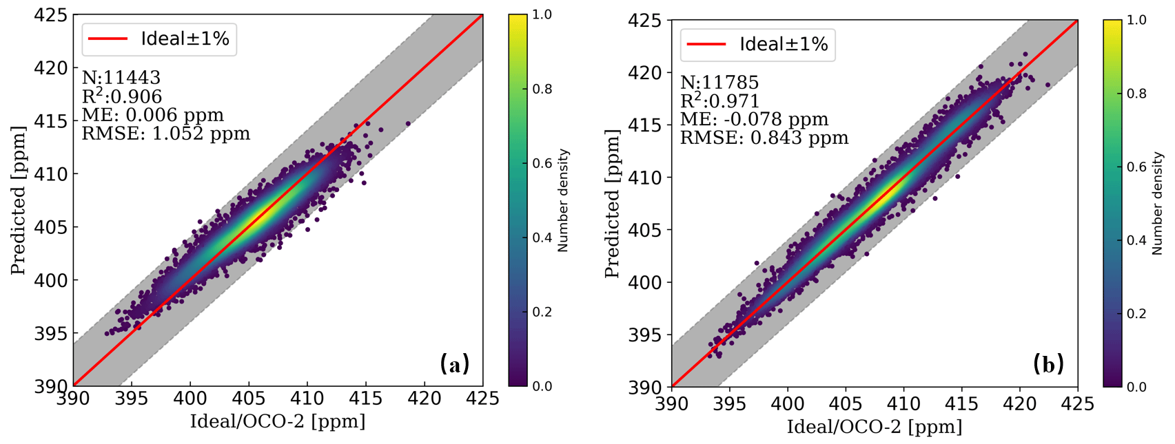
Figure 4Comparison of 10 % out-of-sample XCO2 testing cases predicted by the MLP-XCO2 model versus results retrieved by the OCO-2 v10r product. Panel (a) is the historical data training model, while panel (b) is the skipped-year training model. The solid red lines in the figure correspond to perfect agreement, and shaded areas around the solid red lines represent ±1 % of XCO2 deviations.
We first developed the MLP-XCO2 model using the OCO-2 v10r product dataset. The primary goal was to optimize the hyperparameters of the MLP-XCO2 network. On one hand, we aimed to confirm whether the “slow bias” shown in Bacour et al. (2023) is a universal issue across machine learning models with similar architecture. On the other hand, by fixing the hyperparameters of the MLP-XCO2 network structure, we sought to develop a comparable model using simulated data. In theory, MLP models using identical hyperparameters should possess the same fitting and generalization abilities. By first presenting results from a model trained solely on satellite product data, we can demonstrate the limitations of these satellite-data-based models. This then motivates the development of new machine learning strategies to overcome these limitations, as discussed in later sections.
Following the target areas and data screening methods discussed previously, observational data and lists of bad pixels were obtained from the OCO-2 v10r L1B database. Additionally, retrieved surface pressure and XCO2 data were obtained from the L2 std database. Specifically, we obtained data from March, June, September, and December spanning the years 2016 to 2020. This time frame was chosen to provide a comprehensive training and testing set for our analysis. In total, the dataset encompassed 194 150 samples collected over this 5-year period. The year-wise distribution of the samples is as follows: 38 626 samples from 2016, 39 850 from 2017, 35 945 from 2018, 36 452 from 2019, and 43 277 from 2020.
After completing the data collection, we proceeded to construct the MLP-XCO2 model. To balance model complexity and performance, the MLP-XCO2 architecture (Fig. 2) comprises five hidden layers, with 1000, 500, 300, 100, and 20 nodes, respectively. All hidden layers also use Rectified Linear Unit (ReLU) activation functions. The output layer contains a single node to predict XCO2 values, with a linear activation function. Upon developing the MLP-XCO2 model architecture as described in this section, we independently trained two versions of the MLP-XCO2 model, each based on the aforementioned model structure but with different training and testing datasets.
3.1 Historical data training
The first MLP-XCO2 model based on OCO-2 product data was trained using historical XCO2 data collected from 2016 to 2018. The test set for this model comprised product data from the years 2019 and 2020. This setup allowed us to assess the model's predictive performance using a straightforward historical data approach.
3.2 Skipped-year training
The second version of the model was trained using data from the years 2016, 2018, and 2020. The test set for this MLP-XCO2 model included the skipped years 2017 and 2019. This unique approach enabled a clearer and more direct comparison of the potential limitations of relying solely on historical data for future predictions.
Figure 4 presents the results for the two trained MLP-XCO2 models on their respective 10 % out-of-sample testing datasets. Panel (a) illustrates the predictions of the historical data training model from the 2016–2018 data, and panel (b) shows similar predictions for the skipped-year training model. Both models achieve high accuracy on these testing datasets, with a root mean square error (RMSE) close to 1 ppm and an R-squared score (R2) larger than 0.9. These results demonstrate the robust interpolation capabilities of both models within their respective training periods, indicating their effectiveness in handling known observed scenarios.
Figure 5 evaluates the generalization capabilities of each MLP-XCO2 model on testing sets comprising years not included in their respective training datasets. These test sets represent periods outside the range of years used for training. Here, we observed a noticeable positive bias solely in the predictions from the historical data training model. In contrast, the skipped-year training model did not exhibit this bias. Performance remains highly accurate for these out-of-range points, further validating the model's robustness for XCO2 prediction within skipped years.
Globally, the average XCO2 in the atmosphere shows a stable annual increase, with an observed rise of approximately 2–3 ppm yr−1. However, despite the inclusion of the corresponding year in the input layer as a high-correlation parameter, there remains a limitation in capturing the potential rising trend of the atmospheric CO2. This highlights the limitations of models trained solely on historical satellite data, motivating the development of new techniques to incorporate external information about temporal CO2 dynamics.
In the previous section, the MLP-XCO2 model showed excellent interpolation within the training data range but exhibited bias when predicting outside this period. To eliminate this bias, we propose using an accurate forward model to simulate representative training data that cover future atmospheric conditions. If we can pre-generate atmospheric profiles that capture possible future states, and simulate the corresponding spectral radiance using an accurate forward model, the MLP-XCO2 model can pre-learn future satellite observations. This could prevent incremental annual bias and enable accurate XCO2 prediction. The effectiveness of this approach depends on the forward model accuracy and representativeness of the simulated atmospheres (Zhao et al., 2022).
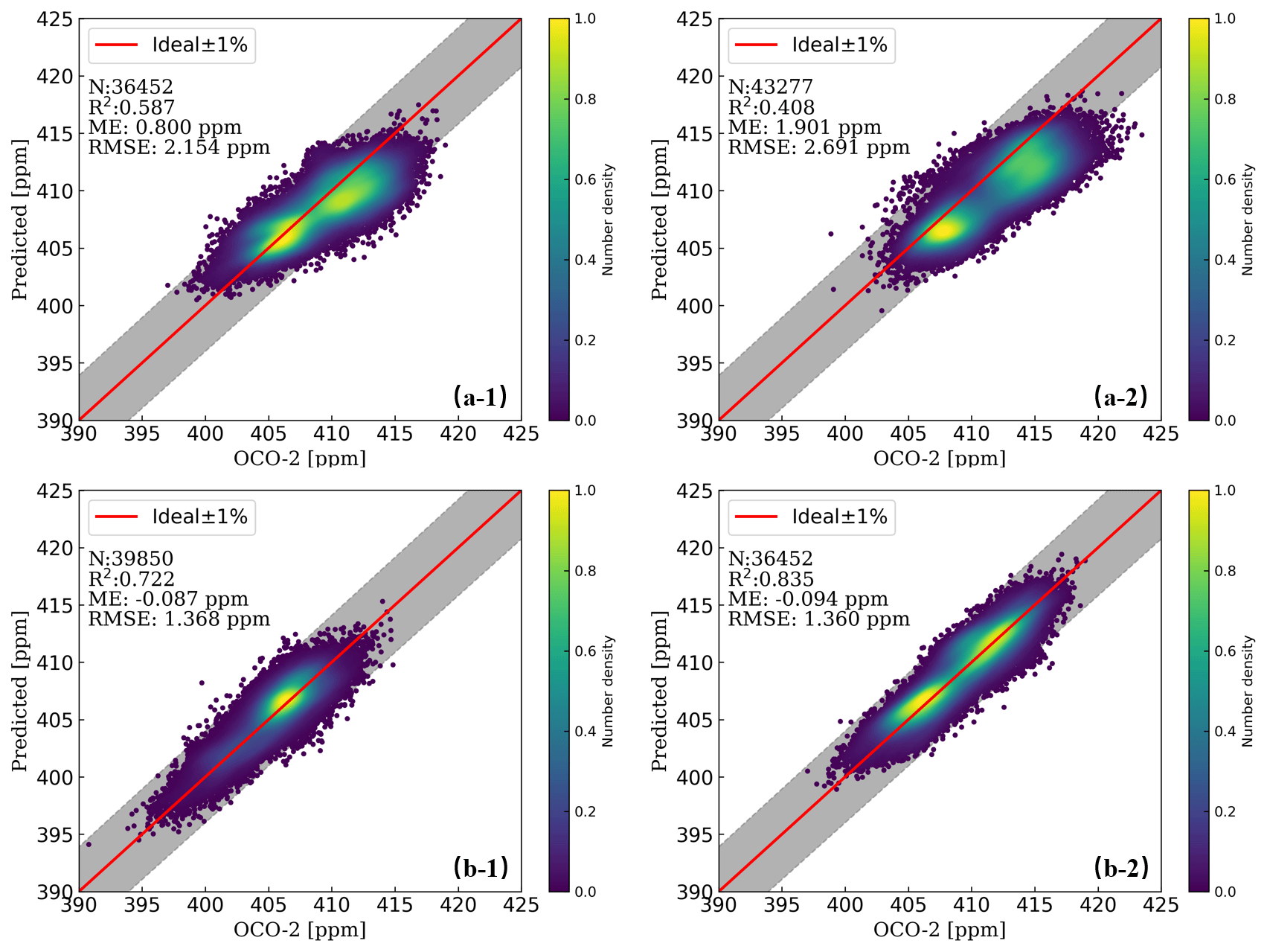
Figure 5Comparison of XCO2 results predicted by the MLP-XCO2 model versus results retrieved by the OCO-2 v10r product on test sets consisting of years not included in the training periods. Panels (a-1) and (a-2) are the historical data training model using the 2019 and 2020 test sets, respectively. Panels (b-1) and (b-2) are the skipped-year training model using the 2017 and 2019 test sets, respectively. The solid red lines in the figure correspond to perfect agreement, and shaded areas around the solid red lines represent ±1 % of XCO2 deviations.
It is therefore critical to select an appropriate radiative-transfer forward model with proven reliability in simulating spectral radiance under varying atmospheric conditions. The model must precisely capture the relationship between trace gas concentrations, meteorological states, and the resulting spectral signatures. With accurate simulations, the machine learning model can generalize robustly to future atmospheric scenarios. The representative training data should span the expected range of atmospheric variability in XCO2 and interfering species like water vapor. A broad sampling of the state space is key for the model to learn a robust mapping to XCO2 across multiple atmospheric regimes. The following sections describe our approach for accurate spectral radiative-transfer simulations and possible (realistic) atmospheric profile generation.
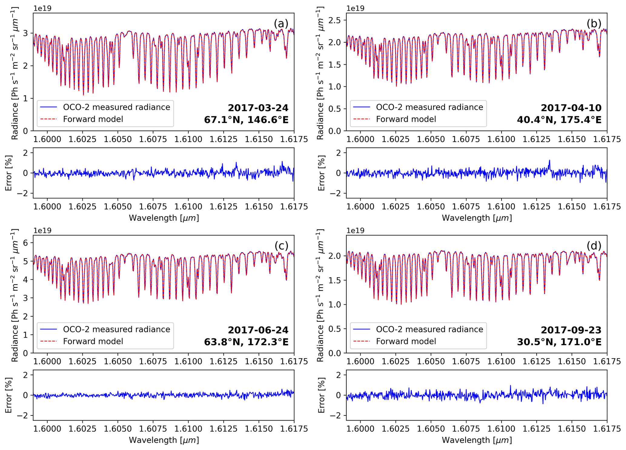
Figure 6Comparisons of the OCO-2 observed spectra with the simulated ones from the modified ReFRACtor forward calculation model in the WCO2 band. The lower subpanel shows the relative error between the spectrum observed by the OCO-2 satellite and that simulated by the forward calculation model. Panels (a)–(d) correspond to test samples from four different regions. The input vectors for the ReFRACtor model were derived from OCO-2 L2std retrieved results.
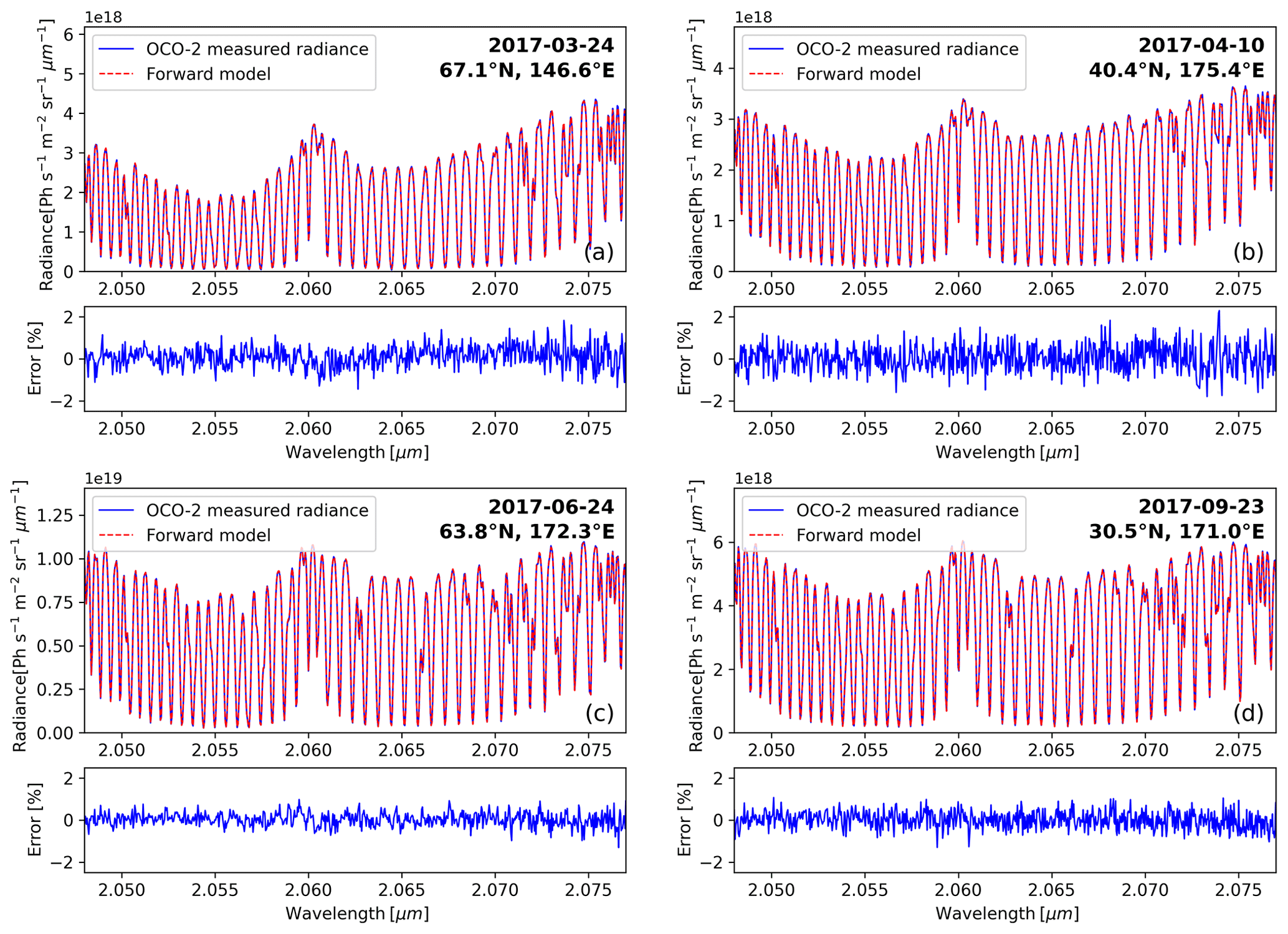
Figure 7Comparisons of the OCO-2 observed spectra with the simulated ones from the corrected ReFRACtor forward calculation model in the SCO2 band. The lower subpanel shows the relative error between the spectrum observed by the OCO-2 satellite and that simulated by the forward calculation model. Panels (a)–(d) correspond to test samples from four different regions. The input vectors for the ReFRACtor model were derived from OCO-2 L2std retrieved results.
4.1 Forward model
In this study, we developed a forward radiative-transfer calculation model using the ReFRACtor (Reusable Framework for Retrieval of Atmospheric Composition) software (McDuffie et al., 2020). ReFRACtor is an extensible framework for multi-instrument atmospheric radiative transfer and retrieval, originally derived from the operational OCO-2 retrieval program. Although ReFRACtor contains both radiative transfer and retrieval capabilities, we only used the radiative-transfer component. Specifically, we configured ReFRACtor to simulate top-of-atmosphere radiance spectra that would be observed by OCO-2. These simulated observations were then used to generate a large training dataset for our machine learning model, MLP-XCO2.
The OCO-2 satellite primarily observes the radiative spectra in the shortwave infrared (SWIR) band. Over the range of SWIR, the impact of thermal emission can be ignored when simulating the spectra (Crisp et al., 2021). To simulate OCO-2's observed spectra in the WCO2 band around 1.6 µm and the SCO2 band around 2.06 µm, the ReFRACtor model numerically solves Eq. (1) of the radiative-transfer equation (RTE; Modest and Mazumder, 2021):
where Iη is the observed spectra, μ is the cosine of the observation zenith angle (e.g., μ=cos θ), τ is the vertical optical depth that can be column-integrated from the molecular absorption coefficients and optical path, ϕ is the azimuthal angle relative to the observation point for the satellite and the sun, and J represents the scattering components and inhomogeneous source term describing both single-scattering and multiple-scattering contributions. The term J in RTE can be expressed as Eq. (2):
where ω is the single-scattering albedo, P is the scattering-phase function, μ′ and ϕ′ are the cosine and azimuth angle of the incident direction angle in each direction, μ0 is the cosine of the solar zenith, and I0 is the solar intensity at the top of the atmosphere.
The ReFRACtor model uses a hybrid model to solve RTE. Specifically, the radiative-transfer software Linearized Discrete Ordinate Radiative Transfer (LIDORT; Spurr, 2008) is applied for the scalar and Jacobian computation. Concurrently, a two-order scattering model (Natraj and Spurr, 2007) is utilized for the additional radiance correction. Within this framework, the ReFRACtor model comprehensively considers five types of scatter particles for each sounding: two types of clouds, two types of tropospheric aerosols, and one type of stratospheric aerosol. The single-scattering optical properties for each cloud and aerosol particle, including cross-section, single-scattering albedo, and scattering-phase matrix, have been pre-computed and tabulated for the forward calculations. Furthermore, the model determines surface reflectance as a quadratic spectral albedo for each band, which is derived from the bidirectional reflectance distribution function (BRDF).
An essential step in developing the forward calculation model is referencing the pre-computed lookup table of H2O and CO2 to obtain the required spectral absorption coefficients. In this study, the ABSCO v5.1 database (absorption coefficient table; Payne et al., 2020) was applied for this purpose. Additionally, we identified and corrected an overestimation of the solar continuum in ReFRACtor compared to the OCO-2 Level 2 algorithm (Crisp et al., 2021). Without this correction, there would have been an approximately 3 % overestimation in the 1.6 µm band and 6.5 % in the 2.06 µm band. By reducing the solar continuum, our forward model aligned better with the OCO-2 spectral measurements. These configurations of the absorption coefficients and solar continuum were essential to accurately simulate OCO-2 spectra for generating training data across a variety of observation conditions.
To assess the performance of the forward model, we selected four distinct global locations in the year 2017. The goal was to replicate the OCO-2-observed spectra for both the WCO2 1.6 µm absorption band and the SCO2 2.06 µm absorption band at the four locations. By accessing the OCO-2 L2 std database, we acquired atmospheric conditions and pertinent geographical data (including spectral albedo, surface pressure, and observation angles) specific to these chosen locations. The outcomes of our simulations for these four locations are visually depicted in Figs. 6 and 7, respectively, for the two bands, with accompanying residual plots displayed in the lower subpanels. It is worth noting that the simulated results exhibit a high level of agreement with the observed OCO-2 spectra; the relative error remains under 1 %, underlining the robustness of the established forward model. The remarkable agreement between the observed and simulated spectra indicates the excellent performance of the forward radiative-transfer model. This performance is particularly evident in accurately replicating the satellite observations from OCO-2. As a result, this forward model serves as a reliable tool for the development of machine learning models trained using simulated spectral data.
4.2 Training data generation
To optimize the training of the MLP-XCO2 model, it is essential that the input training vectors cover a wide range of realistic variations. Although the idea of randomizing all input parameters to enhance diversity might appear attractive, simulating satellite spectra involves managing a multitude of interdependent variables. In addition to the CO2 vertical profile, factors such as surface pressure, temperature profile, water vapor, aerosols, and observation geometry must be accurately represented. Randomizing all of these parameters would require an impractical amount of data and could result in combinations that have no real-world relevance. For example, the four viewing angles determined by the Sun, observation point, and the OCO-2 satellite have fixed combinations during the satellite's regular operation. Therefore, randomly selecting angle combinations lacks practical significance. To ensure that the training data cover valid variations, we conducted an analysis of historical OCO-2 retrievals. This analysis revealed consistent seasonal patterns and year-to-year trends in most parameters. This supports the idea of selecting representative samples from statistical distributions rather than relying on complete randomization. By carefully considering the relationships between parameters and the realities of satellite observations, we can create a reasonably sized training dataset that effectively captures the range of expected predictions.
Generation of the vertical CO2 profile is especially critical among all input parameters. This dataset theoretically determines the generalization domain of the MLP-XCO2 model. In the forward model based on the ReFRACtor model, the atmospheric CO2 profile is segmented into 20 sub-layers by pressure. By statistically analyzing the OCO-2-retrieved CO2 profiles in the target east Asia area in 2016–2018, the boxplots for atmospheric CO2 concentration in each sub-layer are shown in Fig. 8a, and the historic XCO2 results from the OCO-2 product data are shown in Fig. 8b. From the upper atmosphere down to the ground surface, the variability in CO2 concentrations gradually increases. This challenges the model's ability to standardize the atmospheric CO2 profiles, particularly closer to the Earth's surface. Fortunately, a consistent year-on-year rise in CO2 concentrations in each sub-layer has been observed over time. Consequently, in our research, we have proposed a method for generating subsequent CO2 atmospheric profiles. We incrementally increase the CO2 concentration by 2.5 ppm annually, starting from the 2016 OCO-2 retrieved CO2 vertical profile. This approach ensures that we encompass a range of plausible atmospheric CO2 distributions with realistic shapes, enabling the generation of simulated spectra for the designated training years.
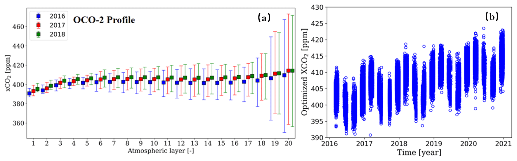
Figure 8Panel (a) is the boxplot of the vertical distribution of CO2 profiles (from OCO-2 L2std files) retrieved by the OCO-2 satellite over east Asia in nadir mode from 2016 to 2018. The horizontal axis represents the atmospheric layers from layer 1 (top of the atmosphere) to layer 20 (near surface). The upper and lower bounds of each whisker show the maximum and minimum CO2 concentrations recorded within that layer for each year. Panel (b) is the scatter plot of historic XCO2 results retrieved by the OCO-2 inversion program (from L2std files).
In addition to the CO2 profile, Fig. 9 illustrates the year-to-year trends of various observed parameters essential for the forward calculation model in the east Asian region. Although they display seasonal variations, these parameters consistently exhibit annually cyclic patterns. Given that the OCO-2 satellite conducts global observations in cycles of approximately half a month (15–16 d), this study employed observation parameters and a priori data for atmospheric profiles, except for CO2, from the year 2016 as a reference. These reference data were repetitively utilized to generate simulations in subsequent years. Regarding the quadratic spectral albedo, the constant term in the training data samples is uniformly set to 1 (to be normalized before being processed by the neural network). The slope and the quadratic coefficient are stochastically sampled within the range of values corresponding to the retrieval results based on the OCO-2 L2 products.
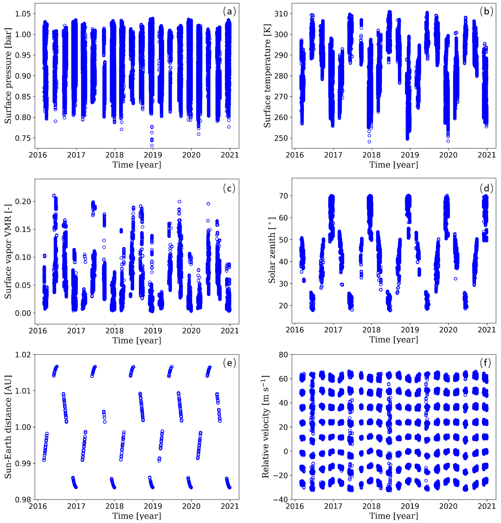
Figure 9Scatter plots of atmospheric parameters required for forward calculation models (excluding CO2 profiles) from 2016 to 2020, sourced from the OCO-2 L2 product. Panel (a) is the surface pressure, (b) is the surface temperature, (c) is the near-surface water vapor concentration, (d) is the solar zenith, (e) is the Sun–Earth distance, and (f) is the Earth–satellite relative velocity.
Based on 60 000 uniformly sampled observation data points exclusively from the OCO-2 satellite throughout 2016, we randomly separated the dataset into six sets of 10 000 data points each. Each set represents CO2 profiles from 2016 to the end of 2021, with the yearly increase of 2.5 ppm added to the original data reflecting projected future profiles. The forward model was used to generate the corresponding simulated spectra for each set. These simulated samples served as the foundational dataset for training the new MLP-XCO2 machine learning model. It is important to note that this new model relies solely on the data recorded by the OCO-2 satellite in 2016 as its reference. However, it is essential to acknowledge that real-world observations by the OCO-2 satellite involve parameters that are not predetermined in future simulations, such as the empirical orthogonal function (EOF) parameters, the signal-to-noise ratio (SNR), bad-sample lists, and the degradation of grating pixels. Therefore, our new model is trained not only on the 60 000 simulated data points but also on the 2016 historical data. According to the data selection criteria outlined in Sect. 2.1, we identified a total of 38 626 sets of historical data in 2016, comprising spectral measurements from OCO-2 and the corresponding XCO2 products. These historical experimental datasets are integrated with the simulated data, enriching the training datasets. These dual combination and data augmentation techniques ensure that the model is well-equipped to handle both potential future atmospheric conditions and the current realities of instrument and spectral measurement capabilities. By doing so, we provide a more comprehensive training strategy that captures both anticipated future scenarios to accurately and efficiently perform XCO2 retrieval for the “future” years from 2017 to the end of 2020.
5.1 Comparison with the OCO-2 satellite product data
To evaluate the retrieval capability of the MLP-XCO2 model trained on a combined dataset of simulated data and historical 2016 OCO-2 satellite data, the neural network architecture and hyperparameters were intentionally kept identical to the previous model trained solely on actual OCO-2 satellite product data. Keeping these factors constant isolates the training data source as the only major difference between the models. This enables a direct, apples-to-apples comparison of how the training data affect model performance.
Figure 10a shows the retrieval results on the 10 % out-of-sample testing data that was excluded from model training. Setting aside this test subset is a standard technique for evaluating model performance on new examples. The accurate predictions of the MLP-XCO2 model for the test data suggest that the model has learned generalizable patterns not overfit to the training data. Figure 10b shows the comparison of the retrieval results of the MLP-XCO2 model to real OCO-2 satellite spectral observations in 2016. Figure 11 displays XCO2 predictions from 2017 to 2020 using test data consistent with Figs. 4 and 5. As the simulated training data were generated based on 2016 OCO-2 measurements, testing on 2017–2020 data evaluates the model's ability to make predictions beyond the time frame of the training data. The scatter plots demonstrate that the MLP-XCO2 model trained on simulated data can accurately and stably predict the annual XCO2 growth trend, maintaining an RMSE less than 1.8 ppm (0.45 %). Compared to models trained relying solely on historical satellite product data, the key advantage is the ability to make reasonable forecasts of future atmospheric XCO2 levels.
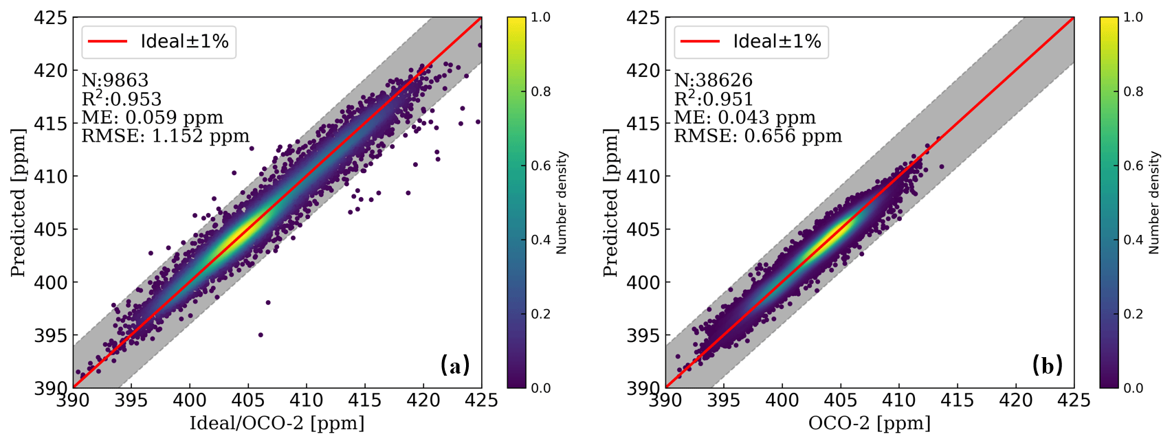
Figure 10Comparison of XCO2 results predicted by the MLP-XCO2 model from the 10 % of test data not involved in training. Panel (a) shows the predicted XCO2 values for the test data that are derived from the simulated dataset, and panel (b) shows the test data that are derived from OCO-2 2016 L2 XCO2 data.
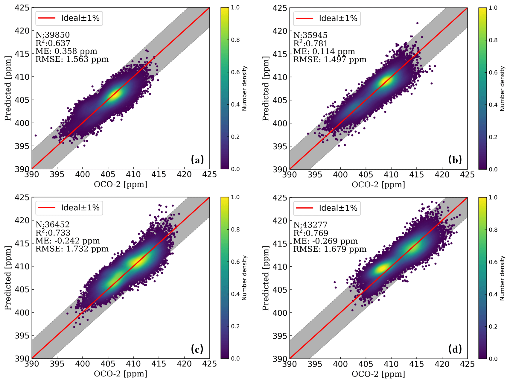
Figure 11Comparison of XCO2 results predicted by the MLP-XCO2 model versus results retrieved by the OCO-2 v10r product in 2017–2020. Panels (a)–(d) display the predictions of the MLP-XCO2 model from 2017 to 2020, respectively.
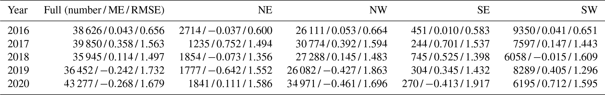
Table 3 offers a detailed spatiotemporal comparison of the results presented in Fig. 11, enhancing our understanding of the MLP-XCO2 model's performance across distinct subregions within east Asia. This table specifically focuses on a finer spatial segmentation within the broad east Asian longitude and latitude range, dividing it into four subregions. These are defined based on the geographical demarcation of 35° N and 130° E, categorized as the northeast (NE), northwest (NW), southeast (SE), and southwest (SW) regions. The results demonstrate that regardless of the distribution of sample sizes across these subregions and their varied topographical characteristics (land or ocean), the model maintains a consistent and stable performance in each subregion. Furthermore, the error metrics for these individual subregions align closely with the overall regional errors, indicating a uniformity in the model's predictive accuracy and reliability across different spatial scales within east Asia.
Table 3Spatiotemporal comparison of XCO2 predicted by MLP-XCO2 model results versus results retrieved by OCO-2 across four subregions. These subregions are delineated based on the geographical demarcation of 35° N and 130° E as the northeast (NE), northwest (NW), southeast (SE), and southwest (SW) regions.
Considering these results, by generating possible realistic future prior information for the atmospheric conditions and using an accurate forward model to simulate the corresponding spectra, the approach avoids inherent biases when extrapolating beyond the distribution of the training data. Rather than simply extending trends, the model is constrained by fundamental physical relationships to interpolate within realistic bounds. This transforms the prediction task into a well-posed interpolation problem instead of an unconstrained extrapolation. The simulated data provide a physical regularization that makes the model's outputs scientifically sound. By training on synthetic data spanning potential future scenarios, the model learns robust representations not tightly coupled to specifics of the training data time period. This enables high-fidelity inversion and prediction of XCO2 even for future time periods beyond available measurements.
5.2 Detecting plume features from the OCO-2 observations
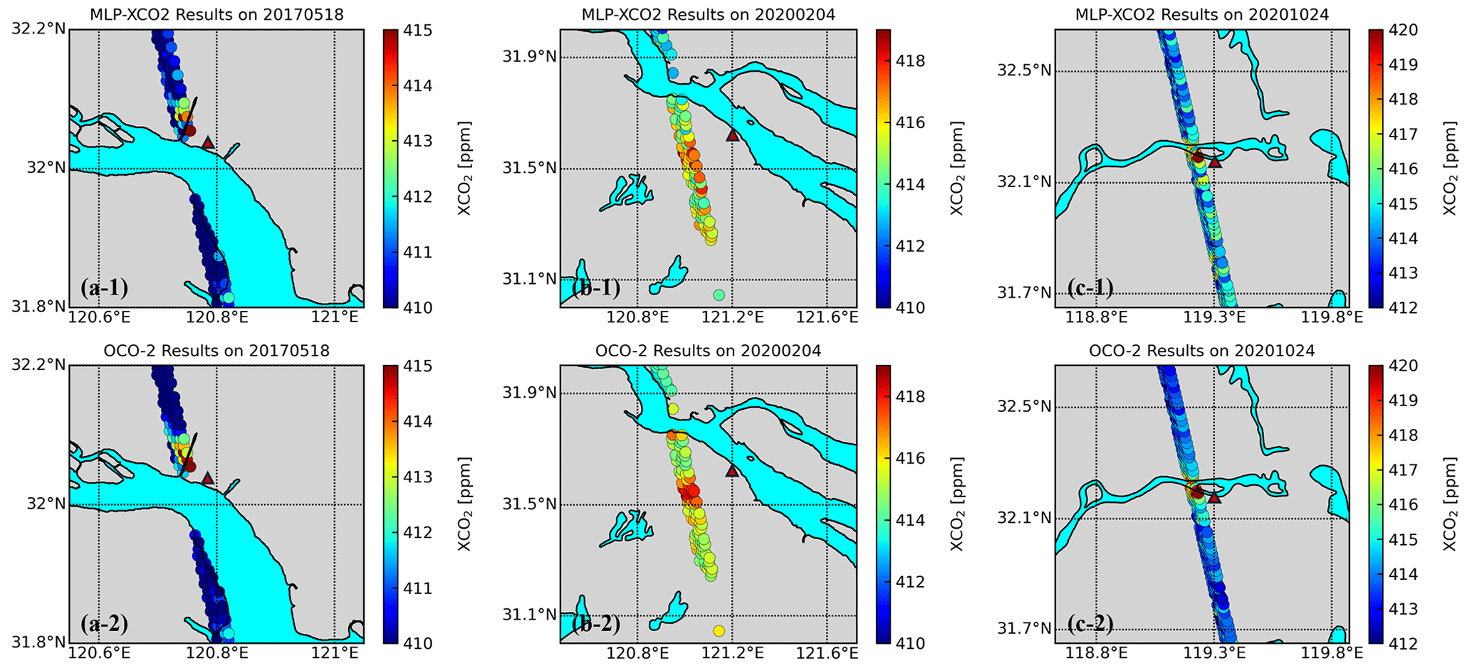
In a further effort to deeply analyze the ability of our MLP-XCO2 model to capture key XCO2 information from spectral data, we focused on plume detection at sites of potentially high emissions, such as thermal power plants, in our target regions from 2017 to 2020. Utilizing the data in the work of Li et al. (2023), we sourced test samples from multiple instances of XCO2 enhancements detected by the OCO-2 satellite in nadir mode observations. These samples were located in close proximity to known large power plants, providing an ideal scenario for assessing retrieval accuracy in detecting localized emission sources.
Figure 12 presents a geographical map that highlights XCO2 predictions in the test samples from the MLP-XCO2 model and compares them with results retrieved by the OCO-2 v10r product. This map clearly marks power plants with red triangles, establishing a visual link between industrial emission sources and observed points where elevated XCO2 levels are detected. Figure 13 further explores this relationship by presenting a longitude-based comparison of XCO2 results. This figure plots the same data points from Fig. 12 against their corresponding longitude coordinates. This arrangement facilitates a direct and intuitive comparison of the trends in XCO2 enhancements captured by our model and reported by the OCO-2 product.
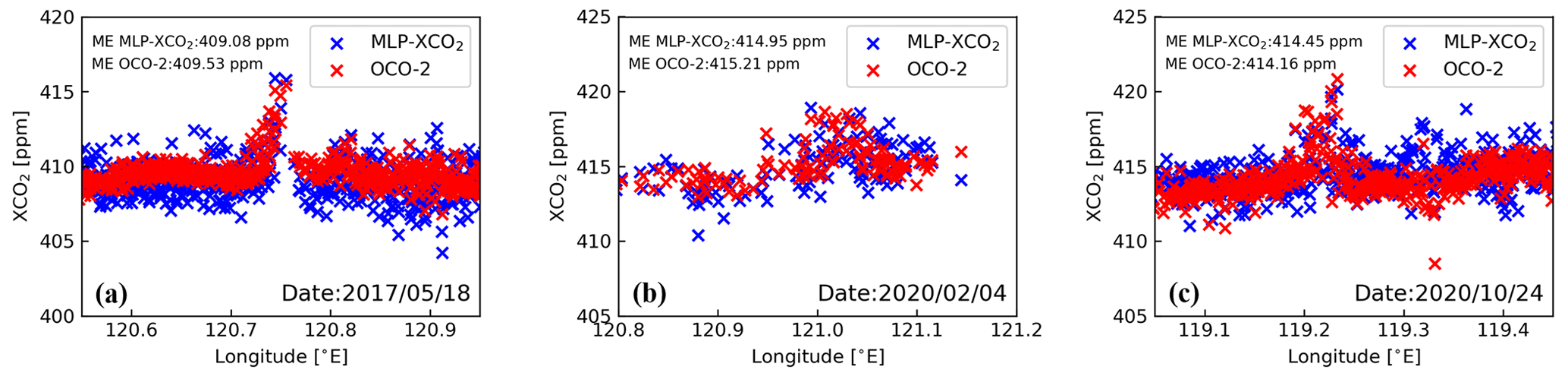
Figure 13Longitude-based scatter comparison of XCO2 predicted by the MLP-XCO2 model versus results retrieved by the OCO-2 v10r product. The potential plume enhancements were screened in nadir mode OCO-2 observations as reported in the work of Li et al. (2023). ME represents the mean value of XCO2 within the longitude range shown in the figure.
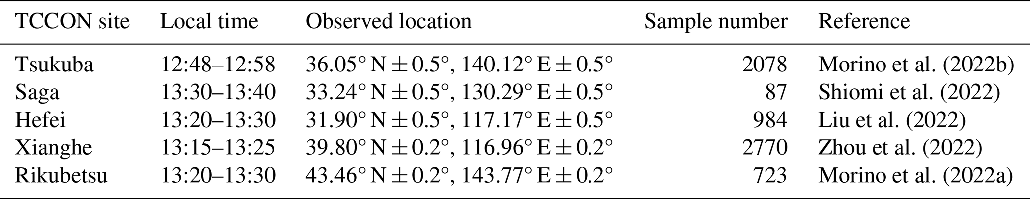
Table 4Spatiotemporal screening conditions for TCCON sites and OCO-2 satellite nadir mode observations.
In both figures, it is visually evident that observation points near power plants show sudden increases in XCO2 values aligning with the trend from the OCO-2 v10r product. This trend is particularly pronounced when compared to points farther away from these emission sources. Considering that these samples are nearly identical in terms of observation angles and times, such consistency is a powerful confirmation of our model's ability to retrieve genuine atmospheric XCO2 from OCO-2 spectral data.
5.3 Comparison with the TCCON data
A comparison of the retrieved results from the OCO-2 satellite showed that the RMSE of our developed MLP-XCO2 model was around 2 ppm. In other words, our results could be worse than or better than the OCO-2 satellite, requiring further comparison with ground-based measurements. To further validate the accuracy of the MLP-XCO2 model, we compared the XCO2 retrievals from the OCO-2 v10r nadir mode products, the MLP-XCO2 model outputs, and ground-based measurements from five TCCON sites within the study region (Fig. 1). As summarized in Table 4, spatiotemporal screening was applied to the TCCON and OCO-2 data to obtain comparable observations. The five TCCON sites included were Tsukuba (Morino et al., 2022b), Saga (Shiomi et al., 2022), Hefei (Liu et al., 2022), Xianghe (Zhou et al., 2022), and Rikubetsu (Morino et al., 2022a). The Anmyeondo site was excluded from this analysis as the XCO2 data were not updated in the TCCON GGG2020 database and were only available until early 2018 in the GGG2014 database.
Figure 14a-1–e-1 presents time series comparisons of XCO2 retrievals from the different TCCON sites, the MLP-XCO2 model, and OCO-2 nadir observations. Figure 14a-2–e-2 displays the boxplots of the differences between the MLP-XCO2 model results, OCO-2 products, and TCCON site data. The plots at each of the five TCCON sites demonstrate that the simulated data-trained MLP-XCO2 model accurately predicts XCO2 from the OCO-2 spectra. The model successfully captures seasonal variations and the long-term XCO2 growth trend over the 4-year study period. The reliable performance over time and across multiple TCCON sites further validates the conclusion that the model has learned generalizable representations of carbon cycle processes rather than overfitting to specifics of the simulated training data. Using realistic future simulations for training, the model provides robust and unbiased XCO2 retrievals across a range of atmospheric conditions.
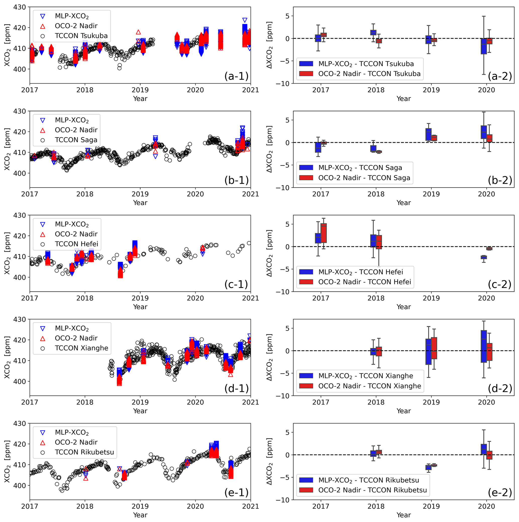
Figure 14Comparisons of XCO2 results from 2017 to 2020 across five TCCON sites. Panels (a-1)–(e-1) show the time series comparisons of XCO2 retrievals from the different TCCON sites, the MLP-XCO2 model, and OCO-2 L2Lite nadir observations for the Tsukuba, Saga, Hefei, Xianghe, and Rikubetsu sites, with data screening conditions as defined in Table 4. Panels (a-2)–(e-2) present the boxplots depicting the differences (ΔXCO2) between the MLP-XCO2 model and OCO-2 products in comparison to the TCCON results for each year. The boxes show the middle half of the data, from the 25th to 75th percentiles. The median (50 %) is represented by the line within each box. The whiskers encompass the central 90 % of the data, extending from the 5th to 95th percentiles.
5.4 Retrieval efficiency
In this study, the ReFRACtor forward model required 12.16 s per simulation case (two absorption bands) using an AMD Ryzen-7 5800X computer. The OCO-2 retrieval based on Bayesian optimization typically needs over three iterations to converge, requiring at least 36.48 s per retrieval. In contrast, the MLP-XCO2 model demonstrated remarkable efficiency on the same hardware. It required just 1.14 s total to retrieve XCO2 from 6642 OCO-2 test spectra across all five TCCON sites, averaging 0.17 ms per sample with an RTX 3080Ti GPU. This rapid inversion drastically reduces processing times compared to traditional methods. While machine learning models need significant upfront time for training data generation and hyperparameter tuning, the prediction is extremely fast once deployed. This enables near-real-time processing ideal for operational satellite data streams. Furthermore, the precision and efficiency of neural networks make them well-suited to meet future demands of high-resolution global greenhouse gas monitoring, enabling millisecond-scale XCO2 retrievals suitable for large-scale satellite analysis.
This proof-of-concept study aims to use the efficient regression inversion capability of the machine learning method to develop machine learning models based on simulated atmospheric radiative-transfer data for efficient inversion of satellite observed spectra to retrieve XCO2. This helps overcome the low efficiency in traditional optimization-based iterative algorithms for XCO2 retrievals. In the present study, XCO2 inversion models using both satellite-product-based data and simulation-based data were developed, trained, and tested. Long time series inversion and prediction of OCO-2 observations over east Asia were also performed using the developed models. The results were compared with OCO-2 and TCCON retrievals, showing that the simulation-data-based machine learning models can effectively eliminate lagging biases while achieving millisecond-level (<1 ms) inversion efficiency, good accuracy (less than 1.8 ppm), local emission source capture, and long-term prediction stability. It should be noted that our current MLP-XCO2 model does not provide direct uncertainty estimates; estimating prediction intervals is an important next step for future improvements. Additionally, to provide good prior information while preventing the model from potentially focusing solely on interpolation rather than learning about actual CO2 increases within spectra, the results of our investigation suggest that integrating additional contextual information, such as the year, can offer valuable context for XCO2 retrieval. However, the underlying mechanisms behind this improvement may require further investigation.
The ReFRACtor model and its OCO retrieval implementation can be accessed from the GitHub ReFRACtor repository (https://doi.org/10.5281/zenodo.4019567, McDuffie et al., 2020). The code and models used in this study have been uploaded to GitHub and can be accessed at https://github.com/TaoRen-Rad/XCO2_retrieval (Xie and Ren, 2024).
The OCO-2 products (including OCO-2 L1B, Met, L2 std, and L2Lite files) are available from the Goddard Earth Sciences Data and Information Services Center (https://disc.gsfc.nasa.gov/datasets/, EarthData, 2023). The TCCON site products are available from TCCON DATA ACHIEVE (https://tccondata.org/, TCCON DATA ACHIEVE, 2023). For access to the dataset, please send requests to Tao Ren (tao.ren@sjtu.edu.cn).
FX and TR designed the study. FX made updates and modifications to the ReFRACtor forward model, developed the machine learning code, and carried out the tests and analysis of the results under the supervision of TR. FX and TR prepared the manuscript. All authors reviewed the final paper.
The contact author has declared that none of the authors has any competing interests.
Publisher's note: Copernicus Publications remains neutral with regard to jurisdictional claims made in the text, published maps, institutional affiliations, or any other geographical representation in this paper. While Copernicus Publications makes every effort to include appropriate place names, the final responsibility lies with the authors.
We gratefully acknowledge the TCCON Data Archive hosted by CaltechDATA at https://tccondata.org (last access: 25 October 2023), as they provided the TCCON data for our study. Our thanks also go to the OCO-2 Science Team for the OCO-2 project. We appreciate our colleagues for their feedback and our affiliated institutions for their unwavering support.
This research has been supported by the National Natural Science Foundation of China (grant nos. 52276077 and 52120105009).
This paper was edited by Abhishek Chatterjee and reviewed by Steffen Mauceri and one anonymous referee.
Bacour, C., Bréon, F.-M., and Chevallier, F.: On the challenge posed by the estimation of XCO2 from OCO-2 observations in near-real time based on artificial neural network, IWGGMS-19, Paris, France, 4–6 July 2023, https://iwggms19.com/wp-content/uploads/2023/05/ID_097_cedric_bacour.pdf (last access: 25 October 2023), 2023. a, b
Bréon, F.-M., David, L., Chatelanaz, P., and Chevallier, F.: On the potential of a neural-network-based approach for estimating XCO2 from OCO-2 measurements, Atmos. Meas. Tech., 15, 5219–5234, https://doi.org/10.5194/amt-15-5219-2022, 2022. a, b
Cansot, E., Pistre, L., Castelnau, M., Landiech, P., Georges, L., Gaeremynck, Y., and Bernard, P.: MicroCarb instrument, overview and first results, in: International Conference on Space Optics – ICSO 2022, edited by: Minoglou, K., Karafolas, N., and Cugny, B., International Society for Optics and Photonics, Dubrovnik, Croatia, 3–7 October 2022, SPIE, 12777, 1277734, https://doi.org/10.1117/12.2690330, 2023. a
Carvalho, A. R., Ramos, F. M., and Carvalho, J. C.: Retrieval of carbon dioxide vertical concentration profiles from satellite data using artificial neural networks, Trends in Computational and Applied Mathematics, 11, 205–216, https://tcam.sbmac.org.br/tema/article/view/90 (last access: 25 October 2023), 2010. a
Chen, T. and Guestrin, C.: Xgboost: A scalable tree boosting system, in: Proceedings of the 22nd ACM Sigkdd International Conference on Knowledge Discovery and Data Mining, 785–794, San Francisco, CA, USA, 13–17 August 2016, https://doi.org/10.1145/2939672.2939785, 2016. a
Cogan, A., Boesch, H., Parker, R., Feng, L., Palmer, P., Blavier, J.-F., Deutscher, N. M., Macatangay, R., Notholt, J., Roehl, C., Warneke, T., and Wunch, D.: Atmospheric carbon dioxide retrieved from the Greenhouse gases Observing SATellite (GOSAT): comparison with ground-based TCCON observations and GEOS-Chem model calculations, J. Geophys. Res.-Atmos., 117, D21301, https://doi.org/10.1029/2012JD018087, 2012. a
Crisp, D., Fisher, B. M., O'Dell, C., Frankenberg, C., Basilio, R., Bösch, H., Brown, L. R., Castano, R., Connor, B., Deutscher, N. M., Eldering, A., Griffith, D., Gunson, M., Kuze, A., Mandrake, L., McDuffie, J., Messerschmidt, J., Miller, C. E., Morino, I., Natraj, V., Notholt, J., O'Brien, D. M., Oyafuso, F., Polonsky, I., Robinson, J., Salawitch, R., Sherlock, V., Smyth, M., Suto, H., Taylor, T. E., Thompson, D. R., Wennberg, P. O., Wunch, D., and Yung, Y. L.: The ACOS CO2 retrieval algorithm – Part II: Global data characterization, Atmos. Meas. Tech., 5, 687–707, https://doi.org/10.5194/amt-5-687-2012, 2012. a
Crisp, D., Pollock, H. R., Rosenberg, R., Chapsky, L., Lee, R. A. M., Oyafuso, F. A., Frankenberg, C., O'Dell, C. W., Bruegge, C. J., Doran, G. B., Eldering, A., Fisher, B. M., Fu, D., Gunson, M. R., Mandrake, L., Osterman, G. B., Schwandner, F. M., Sun, K., Taylor, T. E., Wennberg, P. O., and Wunch, D.: The on-orbit performance of the Orbiting Carbon Observatory-2 (OCO-2) instrument and its radiometrically calibrated products, Atmos. Meas. Tech., 10, 59–81, https://doi.org/10.5194/amt-10-59-2017, 2017. a
Crisp, D., O'Dell, C., Eldering, A., Fisher, B., Oyafuso, F., Payne, V., Drouin, B., Toon, G., Laughner, J., Somkuti, P., McGarragh, G., Merrelli, A., Nelson, R., Gunson, M., Frankenberg, C., Osterman, G., Boesch, H., Brown, L., Castano, R., Christi, M., Connor, B., McDuffie, J., Miller, C., Natraj, V., O’Brien, D., Polonski, I., Smyth, M., Thompson, D., and Granat, R.: Orbiting carbon observatory (OCO)-2 level 2 full physics algorithm theoretical basis document Version 3.0 – Rev 1, https://docserver.gesdisc.eosdis.nasa.gov/public/project/OCO/OCO_L2_ATBD.pdf (last access: 25 October 2023), 2021. a, b
David, L., Bréon, F.-M., and Chevallier, F.: XCO2 estimates from the OCO-2 measurements using a neural network approach, Atmos. Meas. Tech., 14, 117–132, https://doi.org/10.5194/amt-14-117-2021, 2021. a, b
Eldering, A., Taylor, T. E., O'Dell, C. W., and Pavlick, R.: The OCO-3 mission: measurement objectives and expected performance based on 1 year of simulated data, Atmos. Meas. Tech., 12, 2341–2370, https://doi.org/10.5194/amt-12-2341-2019, 2019. a
Gribanov, K., Imasu, R., and Zakharov, V.: Neural networks for CO2 profile retrieval from the data of GOSAT/TANSO-FTS, Atmospheric and Oceanic Optics, 23, 42–47, https://doi.org/10.1134/S1024856010010094, 2010. a
Hamazaki, T., Kaneko, Y., Kuze, A., and Kondo, K.: Fourier transform spectrometer for greenhouse gases observing satellite (GOSAT), in: Enabling sensor and platform technologies for spaceborne remote sensing, Honolulu, Hawai'i, United States, 8–12 November 2004, SPIE, 73–80, 5659, https://doi.org/10.1117/12.581198, 2005. a
Imasu, R., Matsunaga, T., Nakajima, M., Yoshida, Y., Shiomi, K., Morino, I., Saitoh, N., Niwa, Y., Someya, Y., Oishi, Y., Hashimoto, M., Noda, H., Hikosaka, K., Uchino, O., Maksyutov, S., Takagi, H., Ishida, H., Nakajima, T. Y., Nakajima, T., and Shi, C.:Greenhouse gases Observing SATellite 2 (GOSAT-2): mission overview, Progress in Earth and Planetary Science, 10, 33, https://doi.org/10.1186/s40645-023-00562-2, 2023. a
Iwasaki, C., Imasu, R., Bril, A., Oshchepkov, S., Yoshida, Y., Yokota, T., Zakharov, V., Gribanov, K., and Rokotyan, N.: Optimization of the Photon Path Length Probability Density Function-Simultaneous (PPDF-S) Method and Evaluation of CO2 Retrieval Performance Under Dense Aerosol Conditions, Sensors, 19, 1262, https://doi.org/10.3390/s19051262, 2019. a
Jin, Z., Tian, X., Han, R., Fu, Y., Li, X., Mao, H., Chen, C., and GAO, J.: Tan-Tracker global daily NEE and ocean carbon fluxes for 2015–2019 (TT2021 dataset), https://doi.org/10.11888/Meteoro.tpdc.271317, 2021. a
Keely, W. R., Mauceri, S., Crowell, S., and O'Dell, C. W.: A nonlinear data-driven approach to bias correction of XCO2 for NASA's OCO-2 ACOS version 10, Atmos. Meas. Tech., 16, 5725–5748, https://doi.org/10.5194/amt-16-5725-2023, 2023. a
Kuze, A., Suto, H., Nakajima, M., and Hamazaki, T.: Thermal and near infrared sensor for carbon observation Fourier-transform spectrometer on the Greenhouse Gases Observing Satellite for greenhouse gases monitoring, Appl. Optics, 48, 6716–6733, https://doi.org/10.1364/AO.48.006716, 2009. a
Li, Y., Jiang, F., Jia, M., Feng, S., Lai, Y., Ding, J., He, W., Wang, H., Wu, M., Wang, J., Shen, F., and Zhang, L.: Improved estimation of CO2 emissions from thermal power plants based on OCO-2 XCO2 retrieval using inline plume simulation, Sci. Total Environ., 913, 169586, https://doi.org/10.1016/j.scitotenv.2023.169586, 2023. a, b, c
Liang, A., Gong, W., Han, G., and Xiang, C.: Comparison of satellite-observed XCO2 from GOSAT, OCO-2, and ground-based TCCON, Remote Sens.-Basel, 9, 1033, https://doi.org/10.3390/rs9101033, 2017. a
Liu, C., Wang, W., Sun, Y., and Shan, C.: TCCON data from Hefei, China, Release GGG2020R0, CaltechDATA [data set], https://doi.org/10.14291/tccon.ggg2020.hefei01.R0, 2022. a, b
Liu, Y., Wang, J., Yao, L., Chen, X., Cai, Z., Yang, D., Yin, Z., Gu, S., Tian, L., Lu, N., and Lyu, D.: The TanSat mission: preliminary global observations, Sci. Bull., 63, 1200–1207, https://doi.org/10.1016/j.scib.2018.08.004, 2018. a
Marchetti, Y., Rosenberg, R., and Crisp, D.: Classification of anomalous pixels in the focal plane arrays of Orbiting Carbon Observatory-2 and-3 via machine learning, Remote Sens.-Basel, 11, 2901, https://doi.org/10.3390/rs11242901, 2019. a
Matsunaga, T. and Tanimoto, H.: Greenhouse gas observation by TANSO-3 onboard GOSAT-GW, in: Sensors, Systems, and Next-Generation Satellites XXVI, SPIE, 12264, 86–90, 5–8 September 2022, Berlin, Germany, https://doi.org/10.1117/12.2639221, 2022. a
McDuffie, J., Bowman, K., Hobbs, Jo., Natraj, V., Sarkissian, E., Mike, M. T., and Val, S.: Reusable Framework for Retrieval of Atmospheric Composition (ReFRACtor) (Version 1.09), Zenodo [code], https://doi.org/10.5281/zenodo.4019567, 2020. a, b
Meng, G., Wen, Y., Zhang, M., Gu, Y., Xiong, W., Wang, Z., and Niu, S.: The status and development proposal of carbon sources and sinks monitoring satellite system, Carbon Neutrality, 1, 32, https://doi.org/10.1007/s43979-022-00033-5, 2022. a
Messerschmidt, J., Geibel, M. C., Blumenstock, T., Chen, H., Deutscher, N. M., Engel, A., Feist, D. G., Gerbig, C., Gisi, M., Hase, F., Katrynski, K., Kolle, O., Lavrič, J. V., Notholt, J., Palm, M., Ramonet, M., Rettinger, M., Schmidt, M., Sussmann, R., Toon, G. C., Truong, F., Warneke, T., Wennberg, P. O., Wunch, D., and Xueref-Remy, I.: Calibration of TCCON column-averaged CO2: the first aircraft campaign over European TCCON sites, Atmos. Chem. Phys., 11, 10765–10777, https://doi.org/10.5194/acp-11-10765-2011, 2011. a
Modest, M. F. and Mazumder, S.: Radiative heat transfer, Academic Press, https://doi.org/10.1016/C2018-0-03206-5, 2021. a
Morino, I., Ohyama, H., Hori, A., and Ikegami, H.: TCCON data from Rikubetsu, Hokkaido, Japan, Release GGG2020R0, CaltechDATA [data set], https://doi.org/10.14291/tccon.ggg2020.rikubetsu01.R0, 2022a. a, b
Morino, I., Ohyama, H., Hori, A., and Ikegami, H.: TCCON data from Tsukuba, Ibaraki, Japan, 125HR, Release GGG2020R0, CaltechDATA [data set], https://doi.org/10.14291/tccon.ggg2020.tsukuba02.R0, 2022b. a, b
EarthData: GES DISC, Data Collections, NASA, https://disc.gsfc.nasa.gov/datasets/, last access: 25 October 2023. a
Natraj, V. and Spurr, R. J.: A fast linearized pseudo-spherical two orders of scattering model to account for polarization in vertically inhomogeneous scattering–absorbing media, J. Quant. Spectrosc. Ra., 107, 263–293, https://doi.org/10.1016/j.jqsrt.2007.02.011, 2007. a
Nguyen, H., Katzfuss, M., Cressie, N., and Braverman, A.: Spatio-temporal data fusion for very large remote sensing datasets, Technometrics, Taylor & Francis, 56, 174–185, https://doi.org/10.1080/00401706.2013.831774, 2015. a
OCO-2 Science Team, Gunson, M., and Eldering, A.: OCO-2 Level 1B calibrated, geolocated science spectra, Retrospective Processing V10r, Greenbelt, MD, USA, Goddard Earth Sciences Data and Information Services Center (GES DISC), https://doi.org/10.5067/6O3GEUK7U2JG, 2019. a
OCO-2 Science Team, Gunson, M., and Eldering, A.: OCO-2 Level 2 bias-corrected XCO2 and other select fields from the full-physics retrieval aggregated as daily files, Retrospective processing V10r, Greenbelt, MD, USA, Goddard Earth Sciences Data and Information Services Center (GES DISC), https://doi.org/10.5067/6SBROTA57TFH, 2020a. a
OCO-2 Science Team, Gunson, M., and Eldering, A.: OCO-2 Level 2 geolocated XCO2 retrievals results, physical model, Retrospective Processing V10r, Greenbelt, MD, USA, Goddard Earth Sciences Data and Information Services Center (GES DISC), https://doi.org/10.5067/E4E140XDMPO2, 2020b. a
O'Dell, C. W., Connor, B., Bösch, H., O'Brien, D., Frankenberg, C., Castano, R., Christi, M., Eldering, D., Fisher, B., Gunson, M., McDuffie, J., Miller, C. E., Natraj, V., Oyafuso, F., Polonsky, I., Smyth, M., Taylor, T., Toon, G. C., Wennberg, P. O., and Wunch, D.: The ACOS CO2 retrieval algorithm – Part 1: Description and validation against synthetic observations, Atmos. Meas. Tech., 5, 99–121, https://doi.org/10.5194/amt-5-99-2012, 2012. a, b, c
Payne, V. H., Drouin, B. J., Oyafuso, F., Kuai, L., Fisher, B. M., Sung, K., Nemchick, D., Crawford, T. J., Smyth, M., Crisp, D., Adkins, E., Hodges, J. T., Long, D. A., Mlawer, E. J., Merrelli, A., Lunny, E., and O’Dell, C. W.: Absorption coefficient (ABSCO) tables for the Orbiting Carbon Observatories: version 5.1, J. Quant. Spectrosc. Ra., 255, 107217, https://doi.org/10.1016/j.jqsrt.2020.107217, 2020. a
Rodgers, C. D.: Inverse methods for atmospheric sounding: theory and practice, vol. 2, World Scientific, https://doi.org/10.1142/3171, 2000. a
Shiomi, K., Kawakami, S., Ohyama, H., Arai, K., Okumura, H., Ikegami, H., and Usami, M.: TCCON data from Saga, Japan, Release GGG2020R0, CaltechDATA [data set], https://doi.org/10.14291/tccon.ggg2020.saga01.R0, 2022. a, b
Sierk, B., Fernandez, V., Bézy, J.-L., Meijer, Y., Durand, Y., Courrèges-Lacoste, G. B., Pachot, C., Löscher, A., Nett, H., Minoglou, K., Boucher, L., Windpassinger, R., Pasquet, A., Serre, D., and te Hennepe, F.: The Copernicus CO2M mission for monitoring anthropogenic carbon dioxide emissions from space, in: International Conference on Space Optics–ICSO 2020, Vol. 11852, SPIE, 1563–1580, 30 March–2 April 2021, Antibes, France, https://doi.org/10.1117/12.2599613, 2021. a
Spurr, R.: LIDORT and VLIDORT: Linearized pseudo-spherical scalar and vector discrete ordinate radiative transfer models for use in remote sensing retrieval problems, Light scattering reviews 3: Light scattering and reflection, Springer, Berlin, Heidelberg, 229–275, https://doi.org/10.1007/978-3-540-48546-9_7, 2008. a
TCCON DATA ACHIEVE: Total Carbon Column Observing Network (TCCON), Caltech Library Research Data Repository, https://tccondata.org/ (last access: 25 October 2023), 2023. a
Wunch, D., Toon, G. C., Blavier, J.-F. L., Washenfelder, R. A., Notholt, J., Connor, B. J., Griffith, D. W. T., Sherlock, V., and Wennberg, P. O.: The Total Carbon Column Observing Network, Philos. T. Roy. Soc. A, 369, 2087–2112, https://doi.org/10.1098/rsta.2010.0240, 2011. a
Wunch, D., Toon, G. C., Sherlock, V., Deutscher, N. M., Liu, C., Feist, D. G., and Wennberg, P. O.: The Total Carbon Column Observing Network's GGG2014 Data Version, CaltechDATA, https://doi.org/10.14291/tccon.ggg2014.documentation.r0/1221662, 2015. a
Wunch, D., Wennberg, P. O., Osterman, G., Fisher, B., Naylor, B., Roehl, C. M., O'Dell, C., Mandrake, L., Viatte, C., Kiel, M., Griffith, D. W. T., Deutscher, N. M., Velazco, V. A., Notholt, J., Warneke, T., Petri, C., De Maziere, M., Sha, M. K., Sussmann, R., Rettinger, M., Pollard, D., Robinson, J., Morino, I., Uchino, O., Hase, F., Blumenstock, T., Feist, D. G., Arnold, S. G., Strong, K., Mendonca, J., Kivi, R., Heikkinen, P., Iraci, L., Podolske, J., Hillyard, P. W., Kawakami, S., Dubey, M. K., Parker, H. A., Sepulveda, E., García, O. E., Te, Y., Jeseck, P., Gunson, M. R., Crisp, D., and Eldering, A.: Comparisons of the Orbiting Carbon Observatory-2 (OCO-2) measurements with TCCON, Atmos. Meas. Tech., 10, 2209–2238, https://doi.org/10.5194/amt-10-2209-2017, 2017. a
Xie, F. and Ren, T.: MLP-based XCO2 Retrieval Model for East Asian OCO-2 Nadir Observation (v1.0), Zenodo [code], https://doi.org/10.5281/zenodo.12598972, 2024. a
Yoshida, Y., Kikuchi, N., Morino, I., Uchino, O., Oshchepkov, S., Bril, A., Saeki, T., Schutgens, N., Toon, G. C., Wunch, D., Roehl, C. M., Wennberg, P. O., Griffith, D. W. T., Deutscher, N. M., Warneke, T., Notholt, J., Robinson, J., Sherlock, V., Connor, B., Rettinger, M., Sussmann, R., Ahonen, P., Heikkinen, P., Kyrö, E., Mendonca, J., Strong, K., Hase, F., Dohe, S., and Yokota, T.: Improvement of the retrieval algorithm for GOSAT SWIR XCO2 and XCH4 and their validation using TCCON data, Atmos. Meas. Tech., 6, 1533–1547, https://doi.org/10.5194/amt-6-1533-2013, 2013. a
Zehr, S.: The sociology of global climate change, WIREs Clim. Change, 6, 129–150, https://doi.org/10.1002/wcc.328, 2015. a
Zhao, Z., Xie, F., Ren, T., and Zhao, C.: Atmospheric CO2 retrieval from satellite spectral measurements by a two-step machine learning approach, J. Quant. Spectrosc. Ra., 278, 108006, https://doi.org/10.1016/j.jqsrt.2021.108006, 2022. a, b
Zhou, M., Wang, P., Nan, W., Yang, Y., Kumps, N., Hermans, C., and De Mazière, M.: TCCON data from Xianghe, https://doi.org/10.14291/tccon.ggg2020.xianghe01.R0, 2022. a, b
- Abstract
- Introduction
- The machine-learning-based XCO2 retrieval model
- Satellite-product-data-based machine learning model
- Simulation-data-based machine learning model
- Results and discussions
- Conclusions
- Code availability
- Data availability
- Author contributions
- Competing interests
- Disclaimer
- Acknowledgements
- Financial support
- Review statement
- References